Multi-Step Reinforcement Learning: A Unifying Algorithm
Abstract
Unifying seemingly disparate algorithmic ideas to produce better performing algorithms has been a longstanding goal in reinforcement learning. As a primary example, TD() elegantly unifies one-step TD prediction with Monte Carlo methods through the use of eligibility traces and the trace-decay parameter . Currently, there are a multitude of algorithms that can be used to perform TD control, including Sarsa, -learning, and Expected Sarsa. These methods are often studied in the one-step case, but they can be extended across multiple time steps to achieve better performance. Each of these algorithms is seemingly distinct, and no one dominates the others for all problems. In this paper, we study a new multi-step action-value algorithm called that unifies and generalizes these existing algorithms, while subsuming them as special cases. A new parameter, , is introduced to allow the degree of sampling performed by the algorithm at each step during its backup to be continuously varied, with Sarsa existing at one extreme (full sampling), and Expected Sarsa existing at the other (pure expectation). is generally applicable to both on- and off-policy learning, but in this work we focus on experiments in the on-policy case. Our results show that an intermediate value of , which results in a mixture of the existing algorithms, performs better than either extreme. The mixture can also be varied dynamically which can result in even greater performance.
The Landscape of TD Algorithms
11footnotetext: Authors contributed equally, and are listed alphabetically.Temporal-difference (TD) methods [1998] are an important concept in reinforcement learning (RL) that combines ideas from Monte Carlo and dynamic programming methods. TD methods allow learning to occur directly from raw experience in the absence of a model of the environment’s dynamics, like with Monte Carlo methods, while also allowing estimates to be updated based on other learned estimates without waiting for a final result, like with dynamic programming. The core concepts of TD methods provide a flexible framework for creating a variety of powerful algorithms that can be used for both prediction and control.
There are a number of TD control methods that have been proposed. -learning [1989, 1992] is arguably the most popular, and is considered an off-policy method because the policy generating the behaviour (the behaviour policy), and the policy that is being learned (the target policy) are different. Sarsa [1994, 1996] is the classical on-policy control method, where the behaviour and target policies are the same. However, Sarsa can be extended to learn off-policy with the use of importance sampling [2000]. Expected Sarsa is an extension of Sarsa that, instead of using the action-value of the next state to update the value of the current state, uses the expectation of all the subsequent action-values of the current state with respect to the target policy. Expected Sarsa has been studied as a strictly on-policy method [2009], but in this paper we present a more general version that can be used for both on- and off-policy learning and that also subsumes -learning. All of these methods are often described in the simple one-step case, but they can also be extended across multiple time steps.
The TD() algorithm unifies one-step TD learning with Monte Carlo methods [1988]. Through the use of eligibility traces, and the trace-decay parameter, , a spectrum of algorithms is created. At one end, , exists Monte Carlo methods, and at the other, , exists one-step TD learning. In the middle of the spectrum are intermediate methods which can perform better than the methods at either extreme [1998]. The concept of eligibility traces can also be applied to TD control methods such as Sarsa and -learning, which can create more efficient learning and produce better performance [1995].
Multi-step TD methods are usually thought of in terms of an average of many multi-step returns of differing lengths and are often associated with eligibility traces, as is the case with TD(). However, it is also natural to think of them in terms of individual -step returns with their associated -step backup [1998]. We refer to each of these individual backups as atomic backups, whereas the combination of several atomic backups of different lengths creates a compound backup.
In the existing literature, it is not clear how best to extend one-step Expected Sarsa to a multi-step algorithm. The Tree-backup algorithm was originally presented as a method to perform off-policy evaluation when the behaviour policy is non-Markov, non-stationary or completely unknown [2000]. In this paper, we re-present Tree-backup as a natural multi-step extension of Expected Sarsa. Instead of performing the updates with entirely sampled transitions as with multi-step Sarsa, Tree-backup performs the update using the expected values of all the actions at each transition.
is an algorithm that was first proposed by Sutton and Barto (?) which unifies and generalizes the existing multi-step TD control methods. The degree of sampling performed by the algorithm is controlled by the sampling parameter, . At one extreme () exists Sarsa (full sampling), and at the other () exists Tree-backup (pure expectation). Intermediate values of create algorithms with a mixture of sampling and expectation, and can be interpreted as a way to control the bias-variance trade-off inherent in multi-step TD algorithms.
In this work, on problems with a tabular representation and a problem requiring function approximation, we show that an intermediate value of can outperform the algorithms that exist at either extreme. In addition, we show that can be varied dynamically to produce even greater performance. We limit our discussion of to the atomic multi-step case without eligibility traces, but a natural extension is to make use of compound backups and is an avenue for future research. Furthermore, is generally applicable to both on- and off-policy learning, but for our initial empirical study we examined only on-policy prediction and control problems.
MDPs and One-step Solution Methods
The sequential decision problem encountered in RL is often modeled as a Markov decision process (MDP). Under this framework, an agent and the environment interact over a sequence of discrete time steps . At every time step, the agent receives information about the environment’s state, , where is the set of all possible states. The agent uses this information to select an action, , from the set of all possible actions . Based on the behavior of the agent and the state of the environment, the agent receives a reward, , and moves to another state, , with a state-transition probability , for and .
The agent behaves according to a policy , which is a probability distribution over the set . Through the process of policy iteration [1998], the agent learns the optimal policy, , that maximizes the expected discounted return:
| (1) |
for a discount factor and for continuing tasks, or and equal to the final time step in episodic tasks.
TD algorithms strive to maximize the expected return by computing value functions that estimate the expected future rewards in terms of the elements of the environment and the actions of the agent. The state-value function is the expected return when the agent is in a state and follows policy , defined as . For control, most of the time we focus on estimating the action-value function, which is the expected return when the agent takes an action , in a state , while following a policy , and is defined as:
| (2) |
Equation 2 can be estimated iteratively by observing new rewards, bootstrapping on old estimates of , and using the update rule:
| (3) | ||||
where is the step size parameter. Update rules are also known as backup operations because they transfer information back from future states to the current one. A common way to visualize backup operations is by using backup diagrams such as the ones depicted in Figure 1.
For clarity, the algorithmic ideas in this paper are presented initially as tabular solution methods, but we also extend them to use function approximation, and thus they also serve as approximate solution methods.
The term in brackets in (3):
| (4) |
is also known as the TD error, denoted . TD control methods are characterized by their TD error; for example, the TD error in (4) corresponds to the classic on-policy method known as Sarsa.
Because learning requires a certain amount of exploration, behaving greedily with respect to the estimated optimal policy is often infeasible. Therefore, agents are often trained under -greedy policies for which the agent only chooses the optimal action with a probability and behaves randomly with probability , for . Nevertheless, learning the optimal policy is possible if it is done off-policy. When the agent is learning off-policy, it behaves according to a behavior policy, , while learning a target policy, . This can be achieved by using another TD control method, Expected Sarsa. In contrast with Sarsa, Expected Sarsa behaves according to the behavior policy, but updates its estimate by taking an expectation of over the actions at time , according to the target policy [2009]. For convenience, let the expected action-value be defined as:
| (5) |
Then, the TD error of Expected Sarsa can be written as:
| (6) |
A special case of Expected Sarsa is -learning, where the estimate is updated according to the maximum of over the actions [1989]:
| (7) |
-learning is the resulting algorithm when the target policy of Expected Sarsa is the greedy policy with respect to .
Atomic Multi-Step Algorithms
The TD methods presented in the previous section can be generalized even further by bootstrapping over longer time intervals. This has been shown to decrease the bias of the update at the cost of increasing the variance [1994]. Nevertheless, in many cases it is possible to achieve better performance by choosing a value for the backup length parameter, , greater than one [1998]. We refer to algorithms which make use of a multi-step atomic backup as atomic multi-step algorithms. Just like how one-step methods are defined by their TD error, each atomic multi-step algorithm is characterized by its -step return. For atomic multi-step Sarsa, the -step return is:
| (8) |
where is the estimate of at time , and the subscript range, , denotes the length of the backup. -step Sarsa can be adapted for off-policy learning by introducing an importance sampling ratio term [2000]:
| (9) |
and multiplying it with the TD error to get the following update rule:
| (10) | ||||
where is the time step before the end of the update or before the end of the episode. In the update, the action-values for all other states remain the same – i.e. , and . This update rule is not only applicable for off-policy -step Sarsa, but is a generally useful form for other atomic multi-step algorithms as well. We present the algorithms in this work as general off-policy solution methods, but in the experiments section we evaluate them empirically on-policy only which provides useful insight into their behaviour. We defer the empirical study and comparison of the algorithms in an off-policy setting to future work.
Expected Sarsa can also be generalized to a multi-step method by using the return:
| (11) |
The first states and actions are sampled according to the behaviour policy, as with -step Sarsa, but the last state is backed up according to the expected action-value under the target policy. To make -step Expected Sarsa entirely off-policy, an importance sampling ratio term can also be introduced, but it needs to omit the last time step. The resulting update would be the same as in (10), but would use and the -step return for -step Expected Sarsa from (11).
A drawback to using importance sampling to learn off-policy is that it can create high variance which must be compensated for by using small step sizes; this can slow learning [2000]. In the next section we present a method that is also a generalization of Expected Sarsa, but that can learn off-policy without importance sampling.
Tree-backup
As shown in (11), the TD return of -step Expected Sarsa is calculated by taking an expectation over the actions at the last step of the backup. However, it is possible to extend this idea to every time step of the backup by taking an expectation at every step [2000]. The resulting algorithm is a multi-step generalization of Expected Sarsa that is known as Tree-backup because of its characteristic backup diagram (Figure 1). Moreover, just like Expected Sarsa and Q-learning, this proposed generalization does not require importance sampling to be applied off-policy. Hence, it could be argued that it is a more appropriate generalization of Expected Sarsa to multi-step learning [2018]. Because Expected Sarsa subsumes -learning, Tree-backup can also be thought of as a multi-step generalization of -learning if the target policy is greedy with respect to the action-value function.
Tree-backup has several advantages over -step Expected Sarsa. Tree-backup has the capacity for learning off-policy without the need for importance sampling, reducing the variance due to the importance sampling ratios. Additionally, because an importance sampling ratio does not need to be computed, the behavior policy does not need to be stationary, Markov, or even known [2000].
Each branch of the tree represents an action, while the main branch represents the action taken at time . The value of each of the branches is the value of for the corresponding , whereas the value of each segment of the main branch is the reward at the corresponding time step. The -step return is the sum of the values of each branch weighted by the product of the probabilities of the actions leading to the branch and multiplied by the corresponding power of the discount term. For clarity, it is easier to present the -step return of the Tree-backup algorithm in terms of the TD error of Expected Sarsa from (6):
| (12) |
This atomic version of multi-step Tree-backup was first presented by Sutton and Barto (?).
As a result of the product term in (12), in addition to the discount factor , future rewards are further discounted by the probabilities of the actions taken. The Tree-backup algorithm therefore assigns less weight to the reward sequence received, and compensates by bootstrapping off of the values of actions not taken. Due to this, Tree-backup is more biased than Sarsa in the multi-step case with a stochastic policy, as Sarsa gives full weight to every reward received prior to bootstrapping. However, this increase in bias (towards the estimates in the value function) is traded off with decreased variance in the reward sequence from taking expectations.
The Algorithm
In the previous sections we have incrementally introduced several generalizations for the TD control methods Sarsa and Expected Sarsa, and in this section we present an algorithm that unifies them called .
Sarsa can be generalized to an atomic multi-step algorithm by using an -step return, and -step Sarsa generalizes to an off-policy algorithm through the use of importance sampling. In contrast, Expected Sarsa can learn off-policy without the need for importance sampling, and generalizes to the atomic multi-step algorithms: Tree-backup and -step Expected Sarsa. All of the algorithms presented so far can be broadly categorized into two families: those that backup their actions as samples, like Sarsa; and those that consider an expectation over all actions in their backup, like Expected Sarsa and Tree-backup. In this section, we introduce a method to unify both families of algorithms by introducing a new parameter, . The possibility of unifying Sarsa and Tree-backup was first suggested by Precup et al. (?), and the first formulation of was presented by Sutton and Barto (?).
The intuition behind is based on the idea that we have a choice to update the estimate of based on one action sampled from the set of possible future actions, or based on the expectation over the possible future actions. For example, with -step Sarsa, a sample is taken at every step of the backup, whereas with the Tree-backup algorithm, an expectation is taken instead. However, the choice of sampling or expectation does not have to remain constant for every step of the backup. Furthermore, the backup at a time step could be based on a weighted average of both sampling and expectation. In order to implement this, the parameter, , is introduced to control the degree of sampling at each step of the backup. Thus, the TD error of can be represented in terms of a weighted sum of the TD errors of Sarsa and Expected Sarsa:
| (13) |
The -step return is then:
| (14) | ||||
Moreover, the importance sampling ratio from (9) can be modified to include as follows:
| (15) |
The update rule for ) can then be obtained by using from (14) and from (15), with the update rule from (10). Algorithm 1 shows the pseudocode for the complete off-policy -step algorithm.
Additionally, a proof for one-step is readily available by applying the results from Jakkola et al. (?), Singh et al. (?), and van Seijen et al. (?).
Theorem 1.
The one-step ) estimate defined by
| (16) |
converges to the optimal policy when the following conditions are satisfied:
- 1.
The size of the set is finite.
- 2.
, , w.p. 1 and .
- 3.
The policy is greedy in the limit with infinite exploration.
- 4.
The reward function is bounded.
We defer the full details of the proof to the appendix; however, There are two important results from the proof that are worth emphasizing. First, just as with one-step -learning, Sarsa, and Expected Sarsa, one-step can be used to learn optimal action-value functions. Second, at each time step it is possible to choose a such that the contraction property of the update is less than or equal to the contraction induced by the Sarsa or Expected Sarsa updates. This implies that it is possible to choose at every time step in order to speed up convergence.
It is important to note that every TD control method presented thus far can be obtained with by varying the sampling parameter, ; when , we obtain Sarsa, when , we obtain Expected Sarsa and Tree-backup, and when for every step of the backup except for the last, where , we obtain -step Expected Sarsa. Thus, tuning the hyper-parameter is not strictly necessary since it can be set to a fixed value in order to obtain one of the existing TD control algorithms. Nevertheless, intermediate values of between 0 and 1 create entirely new algorithms that exist somewhere between full sampling and pure expectation and that could result in better performance. Furthermore, does not need to remain constant throughout every episode or even at every time step during an episode or continuing task. could be varied dynamically as a function of time, of the current state, or of some measure of the learning progress. In particular, could also be varied as a function of the episode number, which we investigate in our experiments. There are potentially a variety of effective schemes for choosing and varying , and would be a subject for further research.
Experiments
19-State Random Walk
The 19-state random walk, shown in Figure 2, is a 1-dimensional environment where an agent randomly transitions to one of two neighboring states. There is a terminal state on each end of the environment, transitioning to one of them gives a reward of -1, and transitioning to the other gives a reward of 1. To compare algorithms that involve taking an expectation based on its policy, the task is formulated such that each state had two actions. Each action deterministically transitions to one of the two neighboring states, and the agent learns on-policy under an equiprobable random behavior policy. This differs from typical random walk setups where each state has one action that will randomly transition to either neighboring state [1998], but the resulting state values are identical.

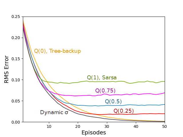
This environment was treated as a prediction task where a learning algorithm is to estimate a value function under its behavior policy. We conducted an experiment comparing various ) algorithm instances, assessing different multi-step backup lengths, step sizes, and degrees of sampling. The root-mean-square (RMS) error between its estimated value function and the analytically computed values was measured after each episode. Each instance and parameter setting ran for 50 episodes and the results are averaged across 100 runs.
Figure 3 shows the results with = 3 and = 0.4, which was found to be representative of the best parameter setting for each instance of on this task. Sarsa (full sampling) had better initial performance but poor asymptotic performance, Tree-backup (no sampling) had poor initial performance but better asymptotic performance, and intermediate degrees of sampling traded off between the initial and asymptotic performances. This motivated the idea of dynamically decreasing from 1 (full sampling) towards 0 (pure expectation) to take advantage of the initial performance of Sarsa, and the asymptotic performance of Tree-backup. To accomplish this we decreased by a factor of 0.95 after each episode. with a dynamically varying outperformed all of the fixed degrees of sampling.
Stochastic Windy Gridworld
The windy gridworld is a tabular navigation task in a standard gridworld which is described by Sutton and Barto (?). There is a start state and a goal state, and there are four possible moves: right, left, up, and down. When the agent moves into one of the middle columns of the gridworld, it is affected by an upward “wind” which shifts the resultant next state upwards by a number of cells and varies from column to column. If the agent is at the edge of the world and selects a move that would cause it to leave the grid, or would be pushed off the world by the wind, it is simply replaced in the nearest state at the edge of the world. At each time step the agent receives a constant reward of -1 until the goal is reached.

A variation of the windy gridworld, called the stochastic windy gridworld, is one where the results of choosing an action are not deterministic. The layout, actions, and wind strengths are the same, but at each time step, with a probability of 10%, the next state that results from picking any action is determined at random from the 8 states currently surrounding the agent.
We conducted an experiment on the stochastic windy gridworld which consisted of 1000 runs of 100 episodes each to evaluate the performance of various instances of with different parameter combinations. All instances of the algorithms behaved and learned according to an -greedy policy, with . As the performance measure, we compared the average return over the 100 episodes. The results are summarized in Figure 4.
For all the values of that we tested, choosing resulted in the greatest performance; higher and lower values of decreased the performance. Overall, ) with a dynamic performed the best, while was a close second.
Mountain Cliff

We implemented a variant of the classical episodic task, mountain car, as described by Sutton and Barto (?). For this implementation, the rewards, actions and goal remained the same. However, if the agent ever ventured past the top of the leftmost mountain, it would fall off a cliff, be rewarded -100 and returned to a random initial location in the valley between the two hills. We named this environment mountain cliff. Both environments were tested and showed the same trend in the results. However, the results obtained in mountain cliff were more pronounced and thus were more suitable for demonstration purposes.
Because the state space is continuous, we approximated using tile coding function approximation. Specifically, we used version 3 of Sutton’s tile coding software (n.d.) with 8 tilings, an asymmetric offset by consecutive odd numbers, and each tile taking over 1/8 fraction of the feature space, which gives a resolution of approximately 1.6%.
For each algorithm, we conducted 500 independent runs of 500 episodes each. All training was done on-policy under an -greedy policy with and . We optimized for the average return after 500 episodes over different values of the step size parameter, , and the backup length, . The results correspond to the best-performing parameter combination for each algorithm: and for Sarsa; and for Tree-backup; and for ; and and for Dynamic . We omit -step Expected Sarsa in the results because its performance was not much different from -step Sarsa’s performance.
Figure 6 shows the return per episode averaged over 500 runs. To smooth the results, we computed a right-centered moving average with a window of 30 successive episodes. Additionally, we added the average return per episode in a lighter tone to show the variance of each algorithm. As it can be observed, atomic multi-step Sarsa and had fairly similar performance. Among the atomic multi-step methods with static , Tree-backup had the best performance. Nonetheless, with dynamic outperformed all the algorithms that were using static .
In order to gain more insight into the nature of the results, we looked at the average return per episode after 50 (initial performance) and 500 (asymptotic performance) episodes for each algorithm. Additionally, a 95% confidence interval was computed in order to validate the results. After 50 episodes, had the best performance among the four algorithms with an average return per episode of -398.0; Dynamic was a close second with an average return per episode of -406.3. On the other hand, after 500 episodes, Dynamic managed to outperform all the other algorithms with an average return per episode of -163.7 followed by with an average return per episode of -167.9. (Sarsa) had the lowest performance with -447.3 average return per episode after 50 episodes and -173.2 after 500 episodes. These results contrast with Figure 6 because the average is taken over all the previous episode instead of the preceding 30 episodes.

Discussion
From our experiments, it is evident that there is merit in unifying the space of algorithms with . In prediction tasks, such as the 19-state random walk, varying the degree of sampling results in a trade-off between initial and asymptotic performance. In control tasks, such as the stochastic windy gridworld, intermediate degrees of sampling are capable of achieving a higher per-episode average return than either extreme, depending on the number of elapsed episodes.
These findings also extend to tasks with continuous state spaces, such as the mountain cliff. Intermediate values of allow for a higher initial performance, whereas small values of allow for a better asymptotic performance. As shown in Figure 6, with dynamic is able to exploit these two benefits by adjusting over time.
Moreover, our experiments in the stochastic windy gridworld task demonstrated that it is possible to improve performance by choosing a higher value of the backup length parameter, . Varying controls a bias-variance trade-off by adjusting how many rewards are included in the backup before bootstrapping, similar to the parameter in the TD() algorithm. The parameter also has a bias-variance trade-off interpretation, as the Tree-backup algorithm decays the weighting of future rewards based on the stochasticity in the policy (and is therefore more biased). The length parameter controls the bias-variance trade-off in the direction of the trajectory taken, while the parameter manages it by controlling the bootstrapping in the direction of actions not taken. A qualitative result that illustrates the bias-variance trade-off induced by the parameter can be observed in the 19-State Random Walk experiment. A large value of results in lower bias at the beginning of training and a lower RMS error as a consequence. However, as the bias of the return decreases in the asymptote, the low variance inherent to small values of result in more accurate estimates of the action-value function.
Conclusions
In this paper we studied , which is a unifying algorithm for multi-step TD control methods. , through the use of the sampling parameter , allows for continuous variation between updating based on full sampling and updating based on pure expectation. Our results on prediction and control problems showed that an intermediate fixed degree of sampling can outperform the methods that exist at the extremes (Sarsa and Tree-backup). In addition, we presented simple way of dynamically adjusting which outperformed any fixed degree of sampling.
Our presentation of was limited to the atomic multi-step case without eligibility traces, we only conducted experiments on on-policy problems, and we only investigated one simple method for dynamically varying . This leaves open several avenues for future research. First, could be extended to use eligibility traces and compound backups. Second, the performance of could be evaluated on off-policy problems. Third, other schemes for dynamically varying could be investigated – perhaps as a function of state, the recently observed rewards, or some measure of the learning progress.
Acknowledgments
The authors thank Vincent Zhang, Harm van Seijen, Doina Precup, and Pierre-luc Bacon for insights and discussions contributing to the results presented in this paper, and the entire Reinforcement Learning and Artificial Intelligence research group for providing the environment to nurture and support this research. We gratefully acknowledge funding from Alberta Innovates – Technology Futures, Google Deepmind, and from the Natural Sciences and Engineering Research Council of Canada.
Appendix
Proof of Theorem 1
Let , , , and be the optimal action-value function defined as
| (17) |
We define a new stochastic process by subtracting from both sides of equation (16)
and letting , , and . Additionally, let be a sequence of increasing -fields representing the history such that and are -measurable and , , and are -measurable for .
Proving that converges to as is equivalent to showing that converges to as . Consequently, the proof is equivalent to showing that the conditions of lemma 1 from Singh et al. (?) are satisfied for .
Conditions one, two, and three of the lemma are satisfied by the corresponding assumptions of the theorem. Hence, we only need to show that where is the maximum norm, , and goes to with probability 1. By adding and subtracting , using the definition of and the triangle inequality, we can show that
Note that if the policy is greedy and , then . Therefore, goes to as the policy becomes greedy in the limit. Consequently, condition 3 of lemma 1 from Sing et al. (?) is satisfied. Therefore, converges to 0 w.p. 1, which implies that converges to w.p. 1. ∎
References
- [1994] Jaakkola, T.; Jordan, M. I.; and Singh, S. P. 1994. On the convergence of stochastic iterative dynamic programming algorithms. Neural Computation 6(6):1185–1201.
- [2000] Precup, D.; Sutton, R. S.; and Singh, S. 2000. Eligibility traces for off-policy policy evaluation. In Kaufman, M., ed., Proceedings of the 17th International Conference on Machine Learning, 759–766.
- [1994] Rummery, G. A., and Niranjan, M. 1994. On-line Q-learning using connectionist systems. Technical report, CUED/F-INFENG/TR 166, Engineering Department, Cambridge University.
- [1995] Rummery, G. A. 1995. Problem Solving with Reinforcement Learning. Ph.D. Dissertation, Cambridge University.
- [2000] Singh, S.; Jaakkola, T.; Littman, M. L.; and Szepesvári, C. 2000. Convergence results for single-step on-policy reinforcement-learning algorithms. Machine Learning 38(3):287–308.
- [1998] Sutton, R. S., and Barto, A. G. 1998. Reinforcement Learning: An Introduction. Cambridge, Massachusetts: MIT Press.
- [2018] Sutton, R. S., and Barto, A. G. 2018. Reinforcement Learning: An Introduction. 2nd edition. Manuscript in preparation.
- [1988] Sutton, R. S. 1988. Learning to predict by the methods of temporal differences. Machine learning 3(1):9–44.
- [1996] Sutton, R. S. 1996. Generalization in reinforcement learning: Successful examples using sparse coarse coding. In Touretzky, D. S., and Hasselmo, M. E., eds., Advances in Neural Information Processing Systems 8, 1038–1044. MIT Press.
- [2009] van Seijen, H.; van Hasselt, H.; Whiteson, S.; and Wiering, M. 2009. A theoretical and empirical analysis of expected Sarsa. In Proceedings of the IEEE Symposium on Adaptive Dynamic Programming and Reinforcement Learning, 177–184.
- [1992] Watkins, C. J. C. H., and Dayan, P. 1992. Q-learning. Machine learning 8(3-4):279–292.
- [1989] Watkins, C. J. C. H. 1989. Learning from Delayed Rewards. Ph.D. Dissertation, Cambridge University.