Deep Collaborative Learning for Visual Recognition
Abstract
Deep neural networks are playing an important role in state-of-the-art visual recognition. To represent high-level visual concepts, modern networks are equipped with large convolutional layers, which use a large number of filters and contribute significantly to model complexity. For example, more than half of the weights of AlexNet are stored in the first fully-connected layer ( filters).
We formulate the function of a convolutional layer as learning a large visual vocabulary, and propose an alternative way, namely Deep Collaborative Learning (DCL), to reduce the computational complexity. We replace a convolutional layer with a two-stage DCL module, in which we first construct a couple of smaller convolutional layers individually, and then fuse them at each spatial position to consider feature co-occurrence. In mathematics, DCL can be explained as an efficient way of learning compositional visual concepts, in which the vocabulary size increases exponentially while the model complexity only increases linearly. We evaluate DCL on a wide range of visual recognition tasks, including a series of multi-digit number classification datasets, and some generic image classification datasets such as SVHN, CIFAR and ILSVRC2012. We apply DCL to several state-of-the-art network structures, improving the recognition accuracy meanwhile reducing the number of parameters ( fewer in AlexNet).
1 Introduction
Image classification is a fundamental problem in computer vision. With the availability of large-scale image datasets [6] and powerful computational resources such as modern GPUs, it is possible to train a convolutional neural network (CNN) [21] which significantly outperforms the conventional models like the Bag-of-Visual-Words [5].
Most CNN architectures contain convolutional (or fully-connected) layers with a large number of filters, which are designed to capture the increasing number of mid-level or high-level visual concepts. These layers contribute significantly to model complexity. As an example, the first fully-connected layer of AlexNet [21] contains filters, requiring parameters (more than of the parameters used in the entire network). We formulate the function of a convolutional layer as learning a large visual vocabulary, in which each filter is used to detect a specific visual concept via template matching. Note that some previous work trains a large visual vocabulary [17] using the composition of several small ones. This idea is successfully applied to approximate nearest neighbor search [10][50], image classification [34] and retrieval [18]. We borrow this idea to reduce the computational complexity of the convolutional layers.
Our algorithm is named Deep Collaborative Learning (DCL). It is a generalized module which applies to a wide range of network structures. The idea is very simple: a large convolutional layer can be simulated with the combination of several small convolutional layers. As illustrated in Figure 1, DCL is a two-stage module to replace a convolutional layer. At the first stage, we individually construct several convolutional layers with the same spatial resolution. These branches are fused at the second stage, which involves linear weighting followed by element-wise operation at each spatial position. In mathematics, DCL can be explained as an efficient way of constructing a compositional visual vocabulary, in which we spend linear complexity to increase the vocabulary size exponentially.
We evaluate DCL on a wide range of visual recognition tasks. First, we generate a series of multi-digit number classification datasets by pasting random MNIST digits into a fixed spatial layout (see Section 4.1 for details). We keep the number of training images unchanged, although the number of categories grows exponentially. DCL works better than conventional models because of two factors. First, DCL enjoys a lower risk of over-fitting, especially in the scenario that the amount of training data is limited. Second, as shown in visualization, DCL uses different branches to learn complementary visual concepts, so that they can be combined to represent the large but decomposable set of visual categories. We also apply DCL to some state-of-the-art network structures, and achieve high accuracy on some generic recognition tasks, including SVHN, CIFAR and ILSVRC2012.
2 Related Work
2.1 Convolutional Neural Networks
The Convolutional Neural Network (CNN) is a hierarchical model for large-scale visual recognition. It is based on the observation that a network with enough neurons is able to fit complicated image data distribution. Recently, the availability of large-scale training data (e.g., ImageNet [6]) and powerful GPUs make it possible to train deep CNNs [21] which significantly outperform conventional approaches such as the Bag-of-Visual-Words (BoVW) model [5]. A CNN is composed of several stacked layers. In each of them, responses from the previous layer are convoluted with a filter bank and activated by a differentiable non-linearity. Hence, a CNN can be considered as a composite function, which is trained by back-propagating error signals defined by the difference between supervision and prediction at the top layer. Efficient methods were proposed to help CNNs converge faster and prevent over-fitting, such as ReLU activation [21], batch normalization [16], Dropout [14] and DisturbLabel [45]. It is believed that deeper networks may produce better recognition results [36][37][13].
The intermediate responses of CNNs, a.k.a., deep features, serve as effective image descriptions [7]. They can be used in a wide range of computer vision tasks, including image classification [7][46][44], image retrieval [32] and object detection [11]. A discussion of how different CNN configurations impact deep feature performance is available in [3].
2.2 Learning Structured Visual Concepts
We aim at learning structured visual concepts, which is related to two research topics, i.e., part-based compositional models and component-based visual vocabulary construction.
The part-based compositional models play an important role in object recognition and detection. It is motivated by the fact that most objects can be decomposed into some functional sub-pieces named parts. To learn a flexible model to organize these parts, the Deformable Part Model (DPM) [8] optimizes an objective function to consider both unary (appearance) terms and binary terms (spatial relationship) terms. The detected parts are useful for object recognition, especially in the fine-grained scenarios [1][2][9][43]. Part-based models can be integrated into deep convolutional neural networks, either for object recognition [49][41], semantic part detection [39] or human pose estimation [4]. There are also efforts at relating intermediate neural responses to object parts [35][40]. This work focuses on learning structured visual representation. Compared to training a compositional model, we introduce stronger prior to facilitate explicit concept decomposition.
When there is the necessity to construct a very large visual vocabulary, an efficient strategy is to train a set of small vocabularies, and combine them to obtain a large one. Motivated by this idea, Product Quantization (PQ) [17] partitions each vector into segments, trains a small codebook on each segment independently, and approximates a vector by the concatenation of quantized codes. To reduce quantization error, efforts are made to weaken the orthogonal constraints [10], leading to composite quantization methods [31][50]. In this work, we borrow this idea to allow deep networks to simulate a large convolutional filter bank with several smaller ones.
Our work is also closely related to bilinear CNN [28], a recent model which trains pairwise discriminative features and assembles them of matrix multiplication. This works well especially in fine-grained visual recognition, but also brings considerable computational overheads. In comparison, our algorithm makes a reasonable assumption to reduce the computational costs significantly.
3 Deep Collaborative Learning
This section presents the Deep Collaborative Learning (DCL) module. The motivation is to use the combination of several small visual vocabularies to simulate the performance of a large vocabulary. This module is especially useful in replacing a convolutional layer with a large number of filters, e.g., the fully-connected layers used in many network structures.
3.1 Formulation
We start with a hidden network layer . is a 3D neuron cube with neurons, where and are the width and height of the data cube, and is the number of channels. We aim at producing a target layer with neurons. This is originally implemented as a convolutional layer with kernels (filters). Let be a spatial position in the layer , where , and be the index of a output channel, the convolutional operation can be formulated as . Here, is the -th filter, and is the data cube at the layer corresponding to the position . is the ReLU activation function [21].
Instead of constructing filters directly, DCL adopts a compositional strategy to perform this task. This is motivated by some previous work [17][50] in constructing a large vocabulary for high-dimensional visual descriptors. A DCL module consists of two stages, i.e., branch construction and concept fusion.
At the first stage, branch construction, intermediate branches are generated. Each of them, denoted as , has neurons, . For simplicity, we assume these branches have the same spatial resolution as the original output layer , i.e., the set is shared among and all ’s. This is easily implemented by using the same convolutional kernel size and spatial stride. Following the above definitions, the convolutional operation can be denoted as , After this stage, at each positions , we obtain vectors, and the -th of them is .
At the second stage, concept fusion, we combine vectors together at each position individually. Recall that DCL is a replacement of the original convolutional layer, therefore we simply keep the number of output channels, i.e., , unchanged. Thus, we need a mapping function . In practice, this is implemented by fully-connecting each to a -dimensional vector , i.e., , and performing an element-wise multiplication followed by -th root to fuse all ’s together, i.e., . Here, is a weighting matrix with elements, and is a small floating point number to avoid numerical instability in gradient computation.
3.2 Learning Compositional Visual Concepts
We show that DCL is able to learn visual concepts in a compositional manner. We investigate an output unit , so that for all , , thus . Following the formulation and ignoring the term, we have:
We focus on the last term , which is the multiplication of convolutional results on the same input patch . To obtain a positive value, each should be positive, which means that all filters are fired at position . Note that the above formula enumerates all combinations of , or equivalently, we consider compositional filters. Although this number grows exponentially with , the model complexity merely increases linearly.
3.3 Relationship to Other Work
DCL is closely related to the Bilinear-CNN (BCNN) model [28]. Both models are motivated by the need of integrating different sources of visual features. To directly compare to BCNN, we set in DCL. Note that BCNN also specifies a set of spatial positions and uses two pre-trained networks for feature extraction. The difference lies in the method of feature fusion, i.e., the concept combination stage in DCL.
At each spatial position , BCNN extracts two types of features and , respectively, and computes the outer-product . Then, the product is fully-connected to a vector at the next stage with a weight matrix . For an element in , its value is defined as . DCL works in a different manner. After and are computed, they are first fully-connected to the next stage with two weight matrices and , then fused via element-wise multiplication followed by taking the square root. Hence, an element in the vector takes the form .
If holds for any , we have . This means that DCL is a constrained case of BCNN, which assumes the decomposable property of the weights. To illustrate this, we explain the neural responses at the position , i.e., and , as some types of visual attributes. As an example, let and represent color and shape features at the given position, respectively. Consider two colors, red and blue, and two shapes, triangle and square, and their combination produces compound visual concepts. Using BCNN, these four compound concepts may be assigned independent weights. Using DCL, on the other hand, the weights are constrained, e.g., if a red triangle is more important than a red square (i.e., the weight on a triangle is higher than the weight on a square), then a blue triangle is also more important than a blue square. Although this constraint applies to each single filter, the ratio can vary from filter to filter, e.g., in another filter, the weight on a triangle may be lower than the weight on a square. Such an assumption is reasonable, since each filter often focuses on a specific combination of visual attributes, and the preference within one attribute is often independent to the preference of other attributes. This assumption, on the other hand, brings the benefit of a reduced number of parameters. For each of the filters, BCNN requires weights, while DCL only needs . In our experiments, and are always large (e.g., tens or hundreds), thus using DCL leads to a less complicated model and, consequently, less risk of over-fitting.
In another perspective, DCL increases the depth of the network but decreases the number of parameters. This is achieved by decomposing the visual vocabulary in the channel domain. A similar effort is made by VGGNet [36], which uses two consecutive layers to simulate the performance of a layer. This is to decompose the vocabulary in the spatial domain.
3.4 Computational Complexity
We analyze the number of trainable parameters and the computational complexity of the original convolutional layer and DCL. Denote as the kernel size used in original convolution () and each of the intermediate branches (, ). An original convolutional layer requires parameters, and complexity, while a DCL module requires parameters, and complexity. Note that is equivalent to .
We discuss the above inequality for some special cases. If and (a common setting before the fully-connected layers), then , and so we can ignore the second term in the left-hand side yielding . If (a regular case between fully-connected layers where the spatial resolution of convolution is ), the inequality becomes . If we further have , then . In experiments, we always set to guarantee reduced complexity.
3.5 Training a Multi-Branch Model
In training a DCL model with more than two intermediate branches (), the high-order root operation may cause instable numerical issues. To deal with this, we suggest a stochastic training strategy, which is opposite to the original deterministic structure. In each training iteration, we randomly activate out of branches, and temporarily disable other branches. This is to say, we only allow the parameters in the active branches to be trained in each iteration. In the testing phase, we compute the expectation of such random selection. This is done by enumerating all branch pairs and computing the averaged neural responses over all these choices.
Besides the numerical issue, the stochastic strategy brings two benefits. First, the network structure used in each training iteration is different, which helps prevent over-fitting. Second, as goes up, it becomes more difficult for all filters to fire at a spatial position. The stochastic strategy considers a pair of filters at each time, possibly giving a neuron positive response when out of filters are fired. The effectiveness of this strategy is verified in experiments (see Section 4.1.2).
4 Experiments
4.1 Multi-Digit Number Classification
We first evaluate DCL on multi-digit number classification to show its ability in discovering feature co-occurrence.
4.1.1 Dataset Construction
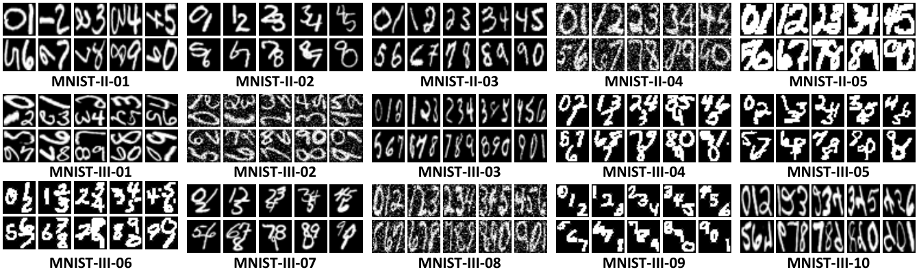
We construct two-digit and three-digit datasets based on the basic MNIST [23]. These datasets differ from each other in many aspects, including the central position of each digit, the scaling, rotation and flipping properties of each digit, and if additional noise is added to the image. We generate the training and testing subsets of each dataset using only the training and testing data of MNIST. Although the number of categories increases significantly ( for two-digit set and for three-digit sets), we keep the amount of training () and testing () images unchanged. This increases the risk of over-fitting for the network models with large numbers of parameters.
The configuration and example images of these multi-digit datasets are shown in Figure 2. When we need to generate a number, we first randomly sample each of its digit from the given (training or testing) set, segment them from the original image, and assemble them into the target image. The geometric property of each digit (i.e., central position, scaling, rotation and flipping) are determined by the fixed configuration of each dataset but may undergo slight random variation. In some cases, neighboring digits may overlap with each other, which increases the difficulty of recognition. Finally, we compute the minimal bounding box of the multi-digit number, and rescale it into (the same size as the original MNIST dataset).
4.1.2 Baseline and Oracle
We use LeNet [22] as our baseline. This is a shallow network with two convolutional layers, two pooling layers and two fully-connected layers. The network architecture can be abbreviated as:
C5@20-MP2S2-C5@50-MP2S2-FC500-D0.5-OUT.
Here, C5@20 is a convolutional layer with a kernel size , a default spatial stride and the number of kernels ; MP2S2 is a max-pooling layer with a kernel size and a spatial stride , FC500 is a fully-connected layer with outputs, and D0.5 is a Dropout layer with a drop ratio . OUT is the output layer, i.e., a fully-connected layer with a proper number ( or ) of filters.
We try different model options and parameters, i.e., replacing different fully-connected layers (the first and/or the second) with DCL, constructing different numbers of branches (two or three), and, in the case of three branches, using either the deterministic or stochastic training strategy as described in Section 3.5. Each branch in DCL contains of the original number of filters. We denote the first and second fully-connected layers as A and B, respectively, and use 2, 3D and 3S to represent training two branches or three branches with different strategies. To summarize, the six DCL models can be denoted as DCL-A2, DCL-A3D, DCL-A3S, DCL-B2, DCL-B3D and DCL-B3S, respectively.
We also compare DCL with the so-called oracle algorithm, which works by training two or three sub-classifiers, each of which for one digit individually, and combining their prediction as the final classification result. Note that this classifier uses strong prior knowledge (each number consists of into several digits), and designs a specific scheme which cannot be generalized to other classification problems. Although it is not fair in direct comparison with DCL, the oracle algorithm provides an upper-bound of the recognition accuracy.
| Dataset | Baseline | Oracle | Deep Collaborative Learning (DCL) | |||||
| A2 | A3S | A3D | B2 | B3S | B3D | |||
| MNIST-II-01 | ||||||||
| MNIST-II-02 | ||||||||
| MNIST-II-03 | ||||||||
| MNIST-II-04 | ||||||||
| MNIST-II-05 | ||||||||
| MNIST-III-01 | ||||||||
| MNIST-III-02 | ||||||||
| MNIST-III-03 | ||||||||
| MNIST-III-04 | ||||||||
| MNIST-III-05 | ||||||||
| MNIST-III-06 | ||||||||
| MNIST-III-07 | ||||||||
| MNIST-III-08 | ||||||||
| MNIST-III-09 | ||||||||
| MNIST-III-10 | ||||||||
Results are summarized in Table 1. First, we observe that the oracle algorithm produces much higher classification accuracy than the baseline model. The benefit mainly comes from the extra knowledge, which decomposes the complicated problem into several sub-classifiers, each of which only needs to distinguish classes, reducing the recognition difficulty significantly. However, such a method cannot be applied to generic classification problems. DCL, on the other hand, does not assume and rely on any extra information, but only designs a compositional structure to facilitate the network to discover feature co-occurrence. Adding DCL on the first fully-connected layer consistently improves the baseline performance on every dataset. In some situations, e.g., MNIST-III-05, the best DCL model is even comparable to the oracle.
4.1.3 Parameters and Complexity
We discuss on the impact of some model options.
- •
The layer replaced by DCL. We find that adding DCL on the first fully-connected layer always outperforms the baseline. Adding DCL on the second fully-connected layer makes the model instable, i.e., sometimes it is significantly better (e.g., MNIST-III-06), sometimes it is even worse than the baseline (e.g., MNIST-II-05). Motivated by this, we do not try to replace two fully-connected layers simultaneously.
- •
The number of branches and the training strategy. On all three-digit datasets, the three-branch models work better than the two-branches models significantly. However, the advantage becomes much smaller when the models are evaluated on two-digit datasets. This suggests that the complexity of the designed structured model should be related to the difficulty of the dataset. We can certainly design a over-complicated model to deal with a simple task, but the increasing number of parameters may incur over-fitting (see later experiments). This is the reason why we do not train models with more than three branches. On the other hand, the stochastic training strategy often works better than the deterministic strategy, which works by randomly switching off branches and reducing the number of parameters in each iteration.
- •
The number of filters in each branch. We evaluate the DCL-A2 model on the most difficult three-digit dataset (MNIST-III-10). Results with respect to different parameters are shown in Figure 4. We can see that the classification accuracy goes up with the increasing amount of filters. However, a large filter bank does not help much in recognition meanwhile brings heavier computational overheads.
In the later experiments on generic classification, we will preserve the best options learned here, i.e., replacing the first fully-connected layer with DCL, using three branches (as natural image often contains complicated situations) with the stochastic training strategy.
Finally, on the most challenging MNIST-III-10 dataset, we plot the training and testing curves of the baseline and three DCL models in Figure 4. Not surprisingly, by reducing the number of parameters, DCL largely alleviates the over-fitting phenomenon in the training process. This is especially useful when the amount of training data is limited.
4.1.4 Learning Complementary Visual Knowledge
We show that DCL is able to learn complementary visual knowledge. To this end, the DCL-A2 and DCL-B2 models trained on the MNIST-II-05 dataset are investigated. We show some statistics of the first filter in each DCL module, including the fused response and the individual responses and . We feed all testing images to these filters, obtain results for , and , respectively. These values grouped using the ground-truth label (the number, the tens digit and the unit digit). In Figure 5, we plot the average responses of on different numbers ( classes) and the average responses of and on different digits ( classes).
We can observe that each fused filter strongly responds to a specific class, and these strong responses come from the individual branches. For example, the fused filter in DCL-A2 learns the visual category 68, thus the corresponding individual filters can learn 6 in the tens digit and 8 in the unit digit, respectively. This makes is possible to implicitly decompose the learning task into smaller and easier ones.
4.2 Generic Image Classification
We show that Deep Collaborative Learning also works well in generic image classification tasks. We evaluate it on four popular datasets, namely SVHN, CIFAR10, CIFAR100, and the large-scale ILSVRC2012 database.
4.2.1 The SVHN and CIFAR Datasets
SVHN (Street View House Numbers) [30] is a large collection of RGB images, i.e., training samples, testing samples, and extra training samples. We preprocess the data as in the previous work [30], i.e., selecting samples per category from the training set as well as samples per category from the extra set, using these images for validation, and the remaining images as training samples. We also use Local Contrast Normalization (LCN) for data preprocessing [12].
CIFAR10 and CIFAR100 [20] are both subsets drawn from the -million tiny image database [38]. There are images for training, and images for testing, all of them are RGB images. CIFAR10 contains basic categories, and CIFAR100 divides each of them into a finer level. In both datasets, training and testing images are uniformly distributed over all the categories. We use exactly the same network configuration as in the SVHN experiments, and add left-right image flipping into data augmentation with the probability .
We use three network structures. The first one is a variant of the LeNet model used in MNIST experiments. The network structure contains three convolutional layers, three pooling layers and two fully-connected layers:
C5(P2)@32-MP3(S2)-C5(P2)@64-MP3(S2)-
C5(P2)@128-MP3(S2)-FC512-D0.5-OUT.
We apply training epochs with learning rate , followed by epochs with learning rate , and another epochs with learning rate .
The second one is named the BigNet, which is borrowed from [29]. In CIFAR datasets, we randomly flip the image with probability. We train the BigNet using samples with learning rate , followed by samples with learning rate and samples with learning rate , respectively. We report a error rate on CIFAR10, comparable to the original version [29], which uses a very complicated way of data preparation and augmentation to get a error rate. Training the original version [29] requires hours, while our model needs only hour. The final baseline, Wide Residual Net (WRN) [47], takes the advantage of deep residual learning [13], and uses a larger number of convolutional kernels and a smaller number of layers. We follow the original implementation to train the -layer WRN, which takes around hours to complete a single model.
| SVHN | CF10 | CF100 | |
|---|---|---|---|
| Zeiler et.al [48] | |||
| Goodfellow et.al [12] | |||
| Lin et.al [27] | |||
| Lee et.al [25] | |||
| Liang et.al [26] | |||
| Lee et.al [24] | |||
| Xie et.al [42] | |||
| Huang et.al [15] | |||
| LeNet (w/o DCL) | |||
| LeNet (w/ DCL) | |||
| BigNet (w/o DCL) | |||
| BigNet (w/ DCL) | |||
| WRN (w/o DCL) | |||
| WRN (w/ DCL) |
Results are summarized in Table 2. We add DCL (two branches, each of which has of the original number of filters) to replace the first fully-connected layer of all three baselines. Consistent accuracy gain is observed. With LeNet, the relative error rate drops are , and on the three datasets; with BigNet, these numbers are , and ; with WRN, these numbers are , and . These experiments verify that DCL generalizes well to both shallow nets (-layer LeNet) and deep nets (-layer BigNet and -layer WRN). Note that DCL achieves accuracy gain with fewer network parameters, e.g., with output nodes, the number of trainable weights in BigNet is shrunk from to ( fewer).
4.2.2 The ILSVRC2012 Dataset
Finally, we evaluate our model on the ImageNet large-scale visual recognition task (the ILSVRC2012 dataset [33] with categories). We use the AlexNet provided by the CAFFE library [19], which is abbreviated as:
C11(S4)@96-MP3(S2)-C5(S1P2)@256-MP3(S2)-
C3(S1P1)@384-C3(S1P1)@384-C3(S1P1)@256-
MP3(S2)-FC4096-D0.5-FC4096-D0.5-FC1000.
The input image is of size , randomly cropped from the original image. Following the setting of CAFFE, a total of mini-batches (approximately epochs) are used for training, each of which has image samples, with the initial learning rate , momentum and weight decay . The learning rate is decreased to after every mini-batches.
We replace the original fc-6 layer ( filters) which two DCL branches, each of which has filters. With DCL, the top- and top- recognition error rates are and , respectively. Comparing to the original rates ( and ), DCL relatively decreases them by about and , respectively. We emphasize that the accuracy gain is not as small as it seems, especially when the number of parameters decreases from to ( fewer) and the average training time per iterations decreases from to ( less).
5 Conclusions
This paper presents Deep Collaborative Learning (DCL), a generalized module which can be plugged into a large family of networks. A DCL module consists of two stages, in which we first build some intermediate branches and then fuse them at each spatial position to consider feature co-occurrence. DCL allows us to construct an exponentially large visual vocabulary with linear complexity, which, in practice, reduces the number of trainable parameters of each model, and alleviates the risk of over-fitting. In experiments, DCL significantly outperforms the baseline model on a series of multi-digit number datasets, and generalizes well to a wide range of generic image classification tasks. We also verify that DCL is able to learn complementary information in different branches.
We learn from DCL that a large filter set can be simulated by several small filter banks. In the current state, DCL works in a fixed decomposition-fusion manner. It would be very interesting to allow neural connections between some small convolutional layers. Meanwhile, other visual tasks, including detection, segmentation, etc., may also benefit from the DCL. The exploration of these topics is left for future work.
References
- [1] T. Berg and P. Belhumeur. POOF: Part-based One-vs.-One Features for Fine-Grained Categorization, Face Verification, and Attribute Estimation. Computer Vision and Pattern Recognition, pages 955–962, 2013.
- [2] Y. Chai, V. Lempitsky, and A. Zisserman. Symbiotic Segmentation and Part Localization for Fine-Grained Categorization. International Conference on Computer Vision, pages 321–328, 2013.
- [3] K. Chatfield, K. Simonyan, A. Vedaldi, and A. Zisserman. Return of the Devil in the Details: Delving Deep into Convolutional Nets. British Machine Vision Conference, 2014.
- [4] X. Chen and A. Yuille. Parsing Occluded People by Flexible Compositions. Computer Vision and Pattern Recognition, 2015.
- [5] G. Csurka, C. Dance, L. Fan, J. Willamowski, and C. Bray. Visual Categorization with Bags of Keypoints. Workshop on Statistical Learning in Computer Vision, European Conference on Computer Vision, 2004.
- [6] J. Deng, W. Dong, R. Socher, L. Li, K. Li, and L. Fei-Fei. ImageNet: A Large-Scale Hierarchical Image Database. Computer Vision and Pattern Recognition, 2009.
- [7] J. Donahue, Y. Jia, O. Vinyals, J. Hoffman, N. Zhang, E. Tzeng, and T. Darrell. DeCAF: A Deep Convolutional Activation Feature for Generic Visual Recognition. International Conference on Machine Learning, 2014.
- [8] P. Felzenszwalb, R. Girshick, D. McAllester, and D. Ramanan. Object Detection with Discriminatively Trained Part-Based Models. IEEE Transactions on Pattern Analysis and Machine Intelligence, 32(9):1627–1645, 2010.
- [9] E. Gavves, B. Fernando, C. Snoek, A. Smeulders, and T. Tuytelaars. Fine-Grained Categorization by Alignments. International Conference on Computer Vision, pages 1713–1720, 2013.
- [10] T. Ge, K. He, Q. Ke, and J. Sun. Optimized Product Quantization for Approximate Nearest Neighbor Search. Computer Vision and Pattern Recognition, 2013.
- [11] R. Girshick, J. Donahue, T. Darrell, and J. Malik. Rich Feature Hierarchies for Accurate Object Detection and Semantic Segmentation. Computer Vision and Pattern Recognition, 2014.
- [12] I. Goodfellow, D. Warde-Farley, M. Mirza, A. Courville, and Y. Bengio. Maxout Networks. International Conference on Machine Learning, 2013.
- [13] K. He, X. Zhang, S. Ren, and J. Sun. Deep Residual Learning for Image Recognition. Computer Vision and Pattern Recognition, 2016.
- [14] G. Hinton, N. Srivastava, A. Krizhevsky, I. Sutskever, and R. Salakhutdinov. Improving Neural Networks by Preventing Co-adaptation of Feature Detectors. arXiv preprint, arXiv: 1207.0580, 2012.
- [15] G. Huang, Y. Sun, Z. Liu, D. Sedra, and K. Weinberger. Deep Networks with Stochastic Depth. European Conference on Computer Vision, 2016.
- [16] S. Ioffe and C. Szegedy. Batch Normalization: Accelerating Deep Network Training by Reducing Internal Covariate Shift. International Conference on Machine Learning, 2015.
- [17] H. Jegou, M. Douze, and C. Schmid. Product Quantization for Nearest Neighbor Search. IEEE Transactions on Pattern Analysis and Machine Intelligence, 33(1):117–128, 2011.
- [18] H. Jegou, F. Perronnin, M. Douze, J. Sanchez, P. Perez, and C. Schmid. Aggregating Local Image Descriptors into Compact Codes. IEEE Transactions on Pattern Analysis and Machine Intelligence, 34(9):1704–1716, 2012.
- [19] Y. Jia, E. Shelhamer, J. Donahue, S. Karayev, J. Long, R. Girshick, S. Guadarrama, and T. Darrell. CAFFE: Convolutional Architecture for Fast Feature Embedding. ACM International Conference on Multimedia, 2014.
- [20] A. Krizhevsky and G. Hinton. Learning Multiple Layers of Features from Tiny Images. Technical Report, University of Toronto, 2009.
- [21] A. Krizhevsky, I. Sutskever, and G. Hinton. ImageNet Classification with Deep Convolutional Neural Networks. Advances in Neural Information Processing Systems, 2012.
- [22] B. LeCun, J. Denker, D. Henderson, R. Howard, W. Hubbard, and L. Jackel. Handwritten Digit Recognition with a Back-Propagation Network. Advances in Neural Information Processing Systems, 1990.
- [23] Y. LeCun, L. Bottou, Y. Bengio, and P. Haffner. Gradient-based Learning Applied to Document Recognition. Proceedings of the IEEE, 86(11):2278–2324, 1998.
- [24] C. Lee, P. Gallagher, and Z. Tu. Generalizing Pooling Functions in Convolutional Neural Networks: Mixed, Gated, and Tree. International Conference on Artificial Intelligence and Statistics, 2016.
- [25] C. Lee, S. Xie, P. Gallagher, Z. Zhang, and Z. Tu. Deeply-Supervised Nets. International Conference on Artificial Intelligence and Statistics, 2015.
- [26] M. Liang and X. Hu. Recurrent Convolutional Neural Network for Object Recognition. Computer Vision and Pattern Recognition, 2015.
- [27] M. Lin, Q. Chen, and S. Yan. Network in Network. International Conference on Learning Representations, 2014.
- [28] T. Lin, A. RoyChowdhury, and S. Maji. Bilinear CNN Models for Fine-Grained Visual Recognition. International Conference on Computer Vision, 2015.
- [29] Nagadomi. The Kaggle CIFAR10 Network. https://github.com/nagadomi/kaggle-cifar10-torch7/, 2014.
- [30] Y. Netzer, T. Wang, A. Coates, A. Bissacco, B. Wu, and A. Ng. Reading Digits in Natural Images with Unsupervised Feature Learning. NIPS Workshop on Deep Learning and Unsupervised Feature Learning, 2011.
- [31] M. Norouzi and D. Fleet. Cartesian k-means. Computer Vision and Pattern Recognition, 2013.
- [32] A. Razavian, H. Azizpour, J. Sullivan, and S. Carlsson. CNN Features off-the-shelf: an Astounding Baseline for Recognition. Computer Vision and Pattern Recognition, 2014.
- [33] O. Russakovsky, J. Deng, H. Su, J. Krause, S. Satheesh, S. Ma, Z. Huang, A. Karpathy, A. Khosla, M. Bernstein, A. Berg, and L. Fei-Fei. ImageNet Large Scale Visual Recognition Challenge. International Journal of Computer Vision, pages 1–42, 2015.
- [34] J. Sanchez, F. Perronnin, T. Mensink, and J. Verbeek. Image Classification with the Fisher Vector: Theory and Practice. International Journal of Computer Vision, 105(3):222–245, 2013.
- [35] M. Simon and E. Rodner. Neural Activation Constellations: Unsupervised Part Model Discovery with Convolutional Networks. International Conference on Computer Vision, 2015.
- [36] K. Simonyan and A. Zisserman. Very Deep Convolutional Networks for Large-Scale Image Recognition. International Conference on Learning Representations, 2014.
- [37] C. Szegedy, W. Liu, Y. Jia, P. Sermanet, S. Reed, D. Anguelov, D. Erhan, V. Vanhoucke, and A. Rabinovich. Going Deeper with Convolutions. Computer Vision and Pattern Recognition, 2015.
- [38] A. Torralba, R. Fergus, and W. Freeman. 80 Million Tiny Images: A Large Data Set for Nonparametric Object and Scene Recognition. IEEE Transactions on Pattern Analysis and Machine Intelligence, 30(11):1958–1970, 2008.
- [39] J. Wang and A. Yuille. Semantic Part Segmentation Using Compositional Model Combining Shape and Appearance. Computer Vision and Pattern Recognition, 2015.
- [40] J. Wang, Z. Zhang, V. Premachandran, and A. Yuille. Discovering Internal Representations from Object-CNNs Using Population Encoding. arXiv preprint arXiv:1511.06855, 2015.
- [41] T. Xiao, Y. Xu, K. Yang, J. Zhang, Y. Peng, and Z. Zhang. The Application of Two-Level Attention Models in Deep Convolutional Neural Network for Fine-Grained Image Classification. Computer Vision and Pattern Recognition, 2015.
- [42] L. Xie, Q. Tian, J. Flynn, J. Wang, and A. Yuille. Geometric Neural Phrase Pooling: Modeling the Spatial Co-occurrence of Neurons. European Conference on Computer Vision, 2016.
- [43] L. Xie, Q. Tian, R. Hong, S. Yan, and B. Zhang. Hierarchical Part Matching for Fine-Grained Visual Categorization. International Conference on Computer Vision, pages 1641–1648, 2013.
- [44] L. Xie, J. Wang, W. Lin, B. Zhang, and Q. Tian. Towards Reversal-Invariant Image Representation. International Journal on Computer Vision, 2016.
- [45] L. Xie, J. Wang, Z. Wei, M. Wang, and Q. Tian. DisturbLabel: Regularizing CNN on the Loss Layer. Computer Vision and Patter Recognition, 2016.
- [46] L. Xie, L. Zheng, J. Wang, A. Yuille, and Q. Tian. InterActive: Inter-Layer Activeness Propagation. Computer Vision and Patter Recognition, 2016.
- [47] S. Zagoruyko and N. Komodakis. Wide Residual Networks. arXiv preprint arXiv:1605.07146, 2016.
- [48] M. Zeiler and R. Fergus. Stochastic Pooling for Regularization of Deep Convolutional Neural Networks. International Conference on Learning Representations, 2013.
- [49] N. Zhang, J. Donahue, R. Girshick, and T. Darrell. Part-based R-CNNs for Fine-Grained Category Detection. European Conference on Computer Vision, 2014.
- [50] T. Zhang, C. Du, and J. Wang. Composite Quantization for Approximate Nearest Neighbor Search. International Conference on Machine Learning, pages 838–846, 2014.