Testing isotropy in the Two Micron All-Sky redshift survey with information entropy
Abstract
We use information entropy to test the isotropy in the nearby galaxy distribution mapped by the Two Micron All-Sky redshift survey (2MRS). We find that the galaxy distribution is highly anisotropic on small scales. The radial anisotropy gradually decreases with increasing length scales and the observed anisotropy is consistent with that expected for an isotropic Poisson distribution beyond a length scale of . Using mock catalogues from N-body simulations, we find that the galaxy distribution in the 2MRS exhibits a degree of anisotropy compatible with that of the CDM model after accounting for the clustering bias of the 2MRS galaxies. We also quantify the polar and azimuthal anisotropies and identify two directions , which are significantly anisotropic compared to the other directions in the sky. We suggest that their preferential orientations on the sky may indicate a possible alignment of the Local Group with two nearby large scale structures. Despite the differences in the degree of anisotropy on small scales, we find that the galaxy distributions in both the 2MRS and the CDM model are isotropic on a scale of .
Keywords:
methods: numerical - galaxies: statistics - cosmology: theory - large scale structure of the Universe.1 Introduction
Our current understanding of the Universe relies on a fundamental assumption that the Universe is statistically homogeneous and isotropic on sufficiently large scales. It is in general difficult to prove this assumption in a strictly mathematical sense but it can be verified using different cosmological observations. Discovery of the Cosmic Microwave Background Radiation (CMBR) in 1964 (Penzias & Wilson, 1965) and the analysis of the data from the COBE mission launched in 1990 revealed that CMBR has a near uniform temperature across the entire sky (Smoot et al., 1992; Fixsen et al., 1996). This discovery provided possibly the most powerful evidence for isotropy. Analysis of data from the two subsequent missions, WMAP launched in 2001 and PLANCK launched in 2009, revealed that CMBR is not completely isotropic. The physics of CMB anisotropy is now well understood. However various studies (Eriksen et al., 2007; Hoftuft et al., 2009; Akrami et al., 2014; Planck Collaboration et al., 2014a; Planck Collaboration et al., 2016b; Schwarz et al., 2004; Land & Magueijo, 2005; Hanson & Lewis, 2009; Moss et al., 2011; Gruppuso et al., 2013; Dai et al., 2013) with WMAP and PLACK reported several unexpected features at large angular scales such as a hemispherical power asymmetry, alignment of the low multipole moments, a preference for the odd parity modes and an unexpectedly large cold spot in the southern hemisphere. Consistency of WMAP and PLANCK results suggest that the instrumental effects are unlikely to produce such features. So the present status of the CMBR observations place the assumption of cosmic isotropy under scanner. The isotropy of the Universe has been favoured by observations in the other wavelengths such as the X-ray background (Wu et al., 1999; Scharf et al., 2000), the angular distributions of radio sources (Wilson & Penzias, 1967; Blake & Wall, 2002) and Gamma-ray bursts (Meegan et al., 1992; Briggs et al., 1996). Some studies on the distribution of supernovae (Gupta & Saini, 2010; Lin et al., 2016), galaxies (Marinoni et al., 2012; Alonso et al., 2015) and neutral hydrogen (Hazra & Shafieloo, 2015) are also consistent with the assumption of statistical isotropy. However there are other studies with Type-Ia supernovae (Schwarz & Weinhorst, 2007; Campanelli et al., 2011; Kalus et al., 2013; Javanmardi et al., 2015; Bengaly et al., 2015), radio sources (Jackson, 2012) and galaxy luminosity function (Appleby & Shafieloo, 2014) which find the evidence for statistically significant deviation from isotropy. The signatures of anisotropy can be also detected using the measurements of large scale bulk flows which are expected to disappear on large scales. Some studies with peculiar velocity surveys, WMAP data and x-ray cluster catalog find statistically significant bulk flows on scales of (Watkins et al., 2009; Kashlinsky et al., 2008; Kashlinsky et al., 2010) whereas some analysis with Type-Ia Supernovae find no evidence of such bulk flows (Huterer et al., 2015). It is also important to understand the origin of any observed anisotropies. There are a number of theoretical studies which predict the level of statistical anisotropy expected from anisotropic inflation (Barrow & Hervik, 2010; Soda, 2012) and backreaction of large scale structure (Marozzi & Uzan, 2012). The Current observational findings suggest that there is no clear consensus on the issue of cosmic isotropy. It is important to test the assumption of isotropy in multiple data sets with different statistical tools. There will be a major paradigm shift in cosmology if different observations rule out the assumption of isotropy with high statistical significance.
The present generation of redshift surveys like 2dFGRS (Colles et al., 2001), SDSS (York et al., 2000) and 2MRS (Huchra et al., 2012) now provide detailed maps of the local Universe. The large sky coverage and the large number of galaxies mapped by these surveys provide an unique opportunity to test the assumption of isotropy in the local universe using galaxy distributions. The 2MASS redshift survey (2MRS) (Huchra et al., 2012) has some unique features which make it distinct compared to the previous optical and far-infrared surveys. The SDSS and 2dFGRS, the two large redshift surveys have not attempted to be complete over the whole sky. The 2MASS redshift survey covers the of the entire sky and selects the galaxies in the near infrared wavelengths around which is less affected by dust extinction and stellar confusion. The near infrared wavelengths are sensitive to the old stellar populations which dominate the galaxy masses and thus provides a statistically uniform galaxy sample in the nearby Universe. The 2MRS survey is complete down to the limiting magnitude and provides a fair sample of the mass distribution in the local Universe. These additional features of the 2MRS make it most suitable for testing isotropy in the local Universe.
Pandey (2016) propose an information theory based method for testing isotropy in a three dimensional distribution. In this paper we apply this method to the all-sky 2MASS redshift survey to test the assumption of cosmic isotropy in the nearby Universe.
A brief outline of the paper follows. We describe our method in Section 2, describe the data in Section 3 and present the results and conclusions in Section 4.
We have used a CDM cosmological model with , and throughout.
2 METHOD OF ANALYSIS
The information entropy is originally introduced by Claude Shannon (Shannon, 1948) in the context of communication of information over a noisy channel. In information theory entropy is the key measure which quantifies the amount of uncertainty involved in the measurement of a random variable. In a more general sense, it gives a measure of the amount of information required to describe a random variable. For a discrete random variable with probability distribution and outcomes , the information entropy associated with is defined as,
| (1) |
Pandey (2016) propose a method to test the isotropy of a three dimensional distribution using information entropy. The method first requires us to identify a galaxy around which isotropy is to be tested. The co-ordinates of the rest of the galaxies are then defined by treating this galaxy as the origin. We carry out an uniform binning of and , where and are respectively the polar angle and azimuthal angle in spherical polar co-ordinates. We adopted this binning so as to ensure equal area for each angular bin. If and bins are used while binning and respectively, it would result in a total angular bins. An upper limit is imposed on the radial co-ordinate as the galaxies are only available within a finite region. We vary the radial co-ordinate within this limit and count the number of galaxies within each volume element defined by the angular bins. For a given value of each of the element has exactly the same volume . Let be the number of galaxies residing inside the volume element. A galaxy within a distance from the centre can only reside in one of the distinct volume elements. One may ask, which particular volume element a randomly selected galaxy belongs to ? There are a total bins and the randomly selected galaxy can reside in any one of them. The probability of finding the randomly selected galaxy in a particular bin would depend on the number of galaxies available in that bin. So we introduce a random variable with outcomes each given by, with the constraint . Here denotes the probability of finding a randomly selected galaxy in the bin. The information entropy associated with for a distance can be written as,
| (2) | |||||
Here is the total number of galaxies within radius . One can choose any base of the logarithm. We choose the base to be for the present work.
In general the probabilities will be different for different elements. The probabilities will have an identical value for all the elements only when they are equally populated. This maximizes the information entropy for a given choice of , and . We define the relative information entropy as the ratio of the entropy of a random variable to its maximum possible value . The relative Shannon entropy quantifies the degree of uncertainty in the knowledge of the random variable . Equivalently we define the residual information which can be considered as a measure of the degree of anisotropy present in the distribution. For an isotropic distribution and consequently .
The galaxies are not randomly distributed. The Gravitational clustering assemble the galaxies into clusters and superclusters which are linked together in a complex filamentary network surrounded by empty regions or voids. The present distribution of galaxies are expected to be highly anisotropic. So the probabilities for different volume elements will be highly non-uniform. If all the galaxies reside in a particular volume element then there will be no uncertainty in identifying the location of the randomly selected galaxy and we will have , . This fully determined situation corresponds to maximum anisotropy and complete lack of information. On the other hand an uniform probability for all the volume elements make it most difficult and uncertain to predict the location of a randomly selected galaxy. This maximizes the information entropy to turning . This corresponds to a distribution which is completely isotropic with maximum amount of information. The galaxy distribution is expected to be anisotropic on small scales but eventually should reach isotropy with increasing size of the angular bins and radius given the assumption of isotropy holds on large scales. We change the value of starting from a small radius and gradually increase it in uniform steps upto its maximum value . We study how varies with for a given choice of and .
Following the definition of the radial anisotropy one can also define similar measures for the polar anisotropy and the azimuthal anisotropy as function of and . For this one needs to carry out the sum over or instead of in Equation 2. It should be noted that in this case in Equation 2 would be the total number of galaxies inside all the or volume elements available at different or respectively. The polar anisotropy quantify the anisotropy among all the bins at each value. Similarly the azimuthal anisotropy quantify the anisotropy among all the bins at each value. We fix the value of at or any desired radius and determine and at different and values respectively. Note that one can also define similar anisotropy measures and and measure them as a function of radius at fixed and respectively. However in the present work we only consider , and to characterize the anisotropies present in the galaxy distribution. We use the galactic co-ordinates throughout the present analysis. So we replace and in the previous definitions by and respectively.
The present day galaxy distribution is highly non-Gaussian. The information entropy is related to the higher order moments of a distribution (Pandey, 2016). So it captures more information about the probability distribution and may serve as a better measure for anisotropies present in a distribution. We would also like to point out here that these measures of anisotropy would never be exactly zero and would be also sensitive to binning and sub-sampling. This relative character of information does not pose any difficulty as it only signifies that the magnitudes of the information is defined with respect to a reference frame and comparison in anisotropies should be always done in the same reference frame. Here we adopt a working definition of isotropy. We compare the anisotropies measured in a distribution with that from Poisson distributions and consider the distribution to be isotropic only when the measured anisotropy lies within the errorbars of the anisotropy expected from a Poisson distribution. We use the same binning and sampling to compute the anisotropies in both the distributions. However for large number of pixels, the size of the volume elements are smaller and consequently the shot noise in an anisotropic distribution may persist upto a larger length scale as compared to a homogeneous and isotropic Poisson random distribution. Our previous definition of isotropy may not apply in such situations. In such cases we consider a distribution to be isotropic when the rate of change of the degree of radial anisotropy with decreases to nearly zero.

3 DATA
3.1 THE 2MRS CATALOGUE
The Two Micron All Sky Redshift Survey (2MRS) (Huchra et al., 2012) provides a three dimensional distribution of galaxies in the nearby Universe. The final survey covers of the sky and is complete to a limiting magnitude of . We download the 2MRS catalogue from http://tdc-www.harvard.edu/2mrs/. The catalog contain galaxies with apparent infrared magnitude and colour excess in the region for and otherwise. We calculate the absolute magnitudes of these galaxies by using their extinction corrected apparent magnitude in the band and applying the k-correction (Kochanek et al., 2001) and e-correction (Branchini et al., 2012) to account for the k-correction and evolutionary correction in the luminosity of the galaxies.
The 2MRS catalog is flux limited. We extract volume limited samples from the 2MRS catalog but find that they are quite sparse and are unsuitable for the present analysis. So we do not apply any absolute magnitude cut but restrict our sample to beyond which there are very few galaxies. The redshift limit is required to simulate the mock catalogues from Poisson random distributions and N-body simulations. We finally have galaxies in our 2MRS sample. We use this flux limited sample for the present analysis.
3.2 REDSHIFT DISTRIBUTION IN THE 2MRS
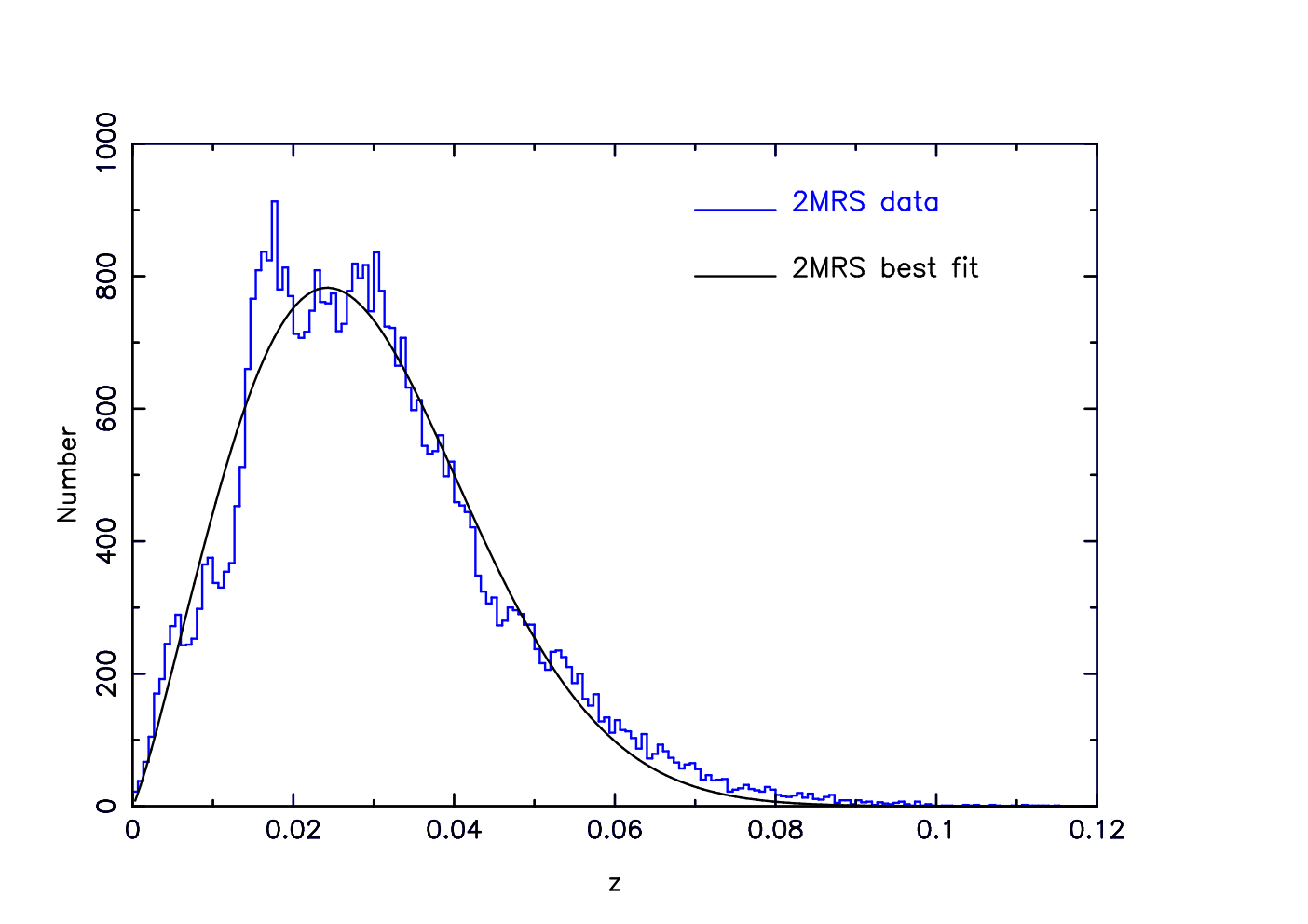
We calculate the redshift distribution of the 2MRS galaxies out to using uniform binsize of . The redshift distribution for the 2MRS sample is shown in the left panel of Figure 1. We model the redshift distribution using a parametrized fit (Erdoǧdu et al., 2006a; Erdoǧdu et al., 2006b) given by,
| (3) |
We find the best fit parameters , , and by fitting the above equation to the 2MRS redshift distribution. The best fit is shown with a smooth solid line in the top left panel of Figure 1. When normalized, the Equation 3 gives the probability of detecting a galaxy at redshift .
3.3 RANDOM CATALOGUES
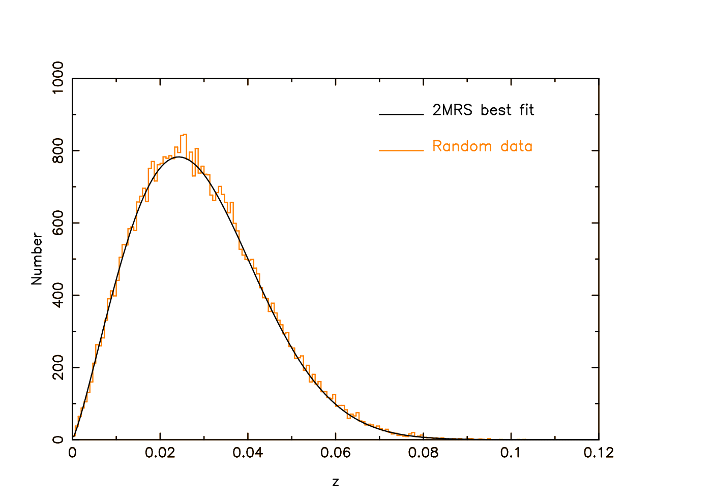
We simulate a set of mock random catalogues for the 2MRS galaxies using Monte Carlo simulation. The maxima of the function in Equation 3 is at . Plugging the best fit values of the parameters , , and yields the maxima at . We calculate the maximum probability by plugging the value of in Equation 3. We randomly choose a redshift in the range and a probability value is randomly chosen in the range . We calculate the actual probability of detecting the galaxy at the selected redshift using Equation 3 and compare it to the randomly selected probability value. If the calculated probability value is larger than the randomly selected probability value, the randomly selected redshift is accepted and assigned isotropically selected galactic co-ordinates and within the sky coverage of the 2MRS survey. We simulate such random mock catalogues. Each random catalogue contains exactly the same number of galaxies distributed over the same region as the actual 2MRS survey. By construction, the random mock catalogues are isotropic around us and they have exactly the same selection function as the 2MASS redshift survey. For comparison, the redshift distribution in a mock random catalogue is shown together with the best fit to the 2MRS data in the top right panel of Figure 1.
3.4 MOCK CATALOGUES FROM N-BODY SIMULATIONS
We simulate the distributions of dark matter in the CDM model using a Particle-Mesh (PM) N-Body code. We use particles on a mesh to simulate the present day distribution of dark matter in a comoving volume of . The following values of the cosmological parameters are used in the simulations: , , , and (Planck Collaboration et al., 2016a). The simulations were run for three different realizations of the initial density fluctuations. We treat the individual particles as galaxies and place an observer at the centre of these boxes. We use the peculiar velocities to produce the galaxy distributions in redshift space and extract mock catalogues for the 2MRS galaxy distribution from each boxes following the same method as used for random distribution. The only difference is that here we do not need to generate isotropically selected galactic co-ordinates for the mock galaxies as these are decided by their co-ordinates. We finally have mock catalogues for the 2MRS galaxies from the N-body simulations of the CDM model.


3.5 FILLING THE ZONE OF AVOIDANCE
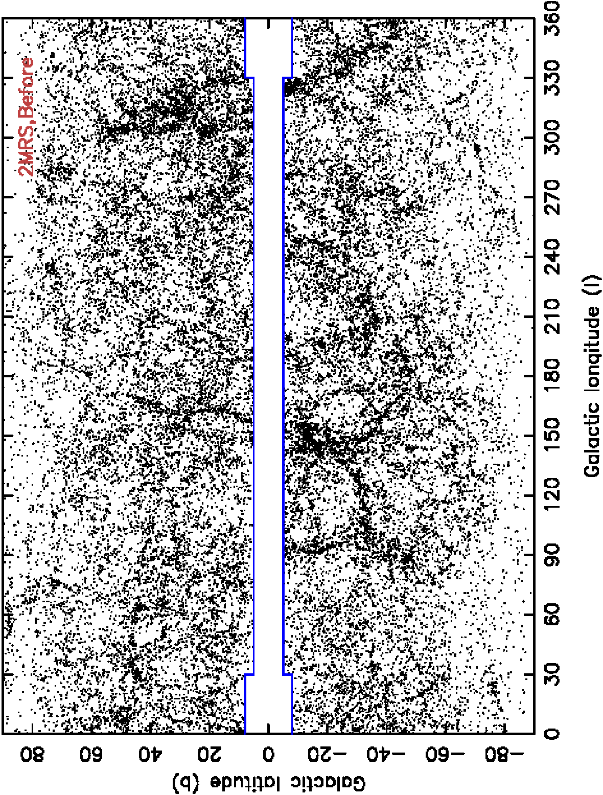
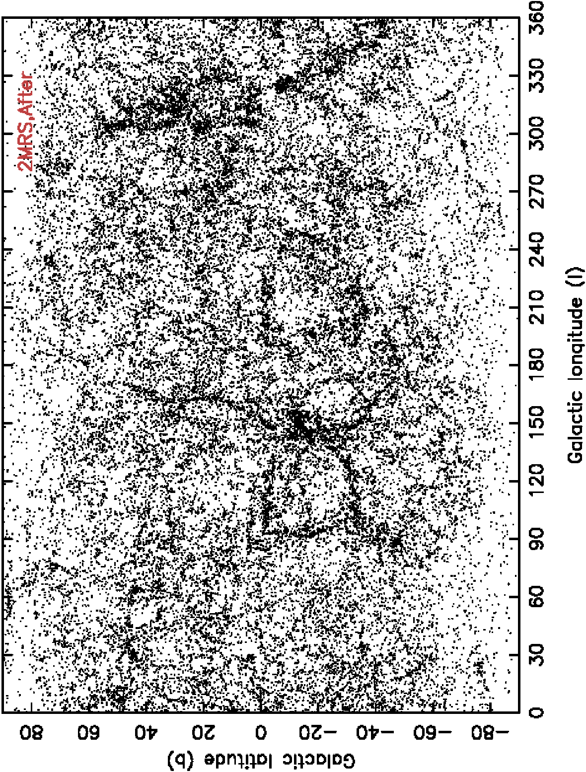
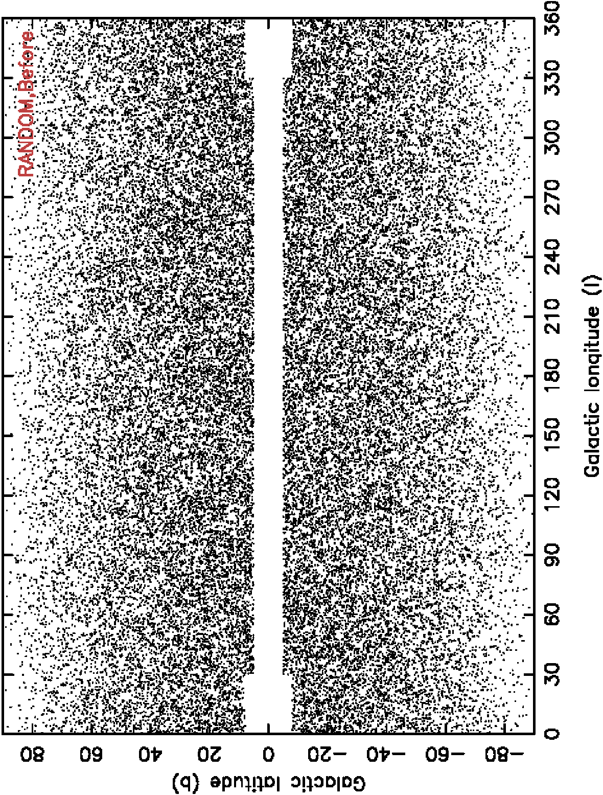
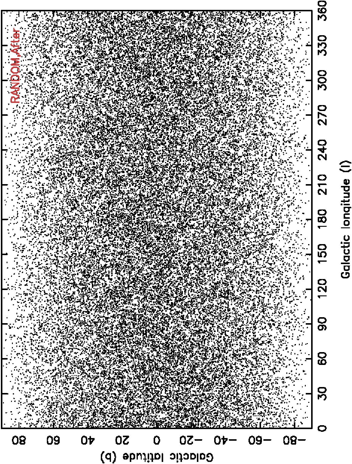
The Zone of Avoidance (ZOA) is the region of the sky near the Galactic plane where the observations are obscured due to the extinction by Galactic dust. The selection in the near infra-red in the 2MRS reduces the impact of the zone of avoidance. Huchra et al. (2012) selected 45,086 2MRS sources which has apparent infrared magnitude and colour excess in the region for and otherwise. They further rejected the sources which are of galactic origin (multiple stars, planetary nebulae, HII regions) and also discarded the sources which are in regions of high stellar density and absorption. After correction for these systematic effects, the final 2MRS catalog provided by Huchra et al. (2012) contain 43,533 galaxies. We use the final 2MRS catalog and the distribution of the 2MRS galaxies in galactic co-ordinates is shown in the top left panel of Figure 2. For a comparison, the distribution for a mock catalogue from random distribution and N-body simulation are also shown in the middle and bottom left panels of the same figure. The ZOA can be clearly identified at the middle of these distributions. The present study aims to explore the isotropy in the observed mass distribution in the local Universe and it would be desirable to have the galaxy distribution over the full sky. We fill the ZOA by randomly cloning individual galaxies from above and below the ZOA (the unmasked region) and then shifting them in latitude to random locations in the masked region so that it finally has the same average density of galaxies as the unmasked region (Lynden-Bell et al., 1989). Although this fails to interpolate the large scale structures across the ZOA, it serves the purpose of constructing a full sky three dimensional galaxy distribution without introducing any spurious signals of anisotropy. We finally have clones filling the ZOA. Our 2MRS sample contains galaxies before filling the ZOA and contains a total galaxies after filling it. Following the same procedure we fill up the ZOA in all the mock catalogues from Poisson random distributions and N-body simulations. After filling the ZOA, the distribution of galaxies in the 2MRS catalogue, a mock random catalogue and a mock catalogue from N-body simulation are shown in the top right, middle right and bottom right panel of Figure 2 respectively.
We note that in reality the zone of avoidance is not as symmetric as defined in Huchra et al. (2012) but as we keep the cloned galaxies in the masked regions and carry out our analysis in coordinate space, we do not expect these to influence our results. We have also checked that filling the zone of avoidance by uniform strips or chunks instead of individual clones does not make any difference to our results. Finally it may be noted that filling the ZOA is not necessary if one limits the analysis to the unmasked regions outside the ZOA.
3.6 JACKKNIFE SAMPLES FOR THE 2MRS
We have only one galaxy sample from the 2MRS. We prepare jackknife samples from the 2MRS data to estimate the errorbars for our measurements. The final 2MRS sample used in this analysis contain galaxies after the ZOA is filled with clones. We used the general delete-m observations jackknife method for equal m. For each of the jackknife samples, we randomly omit galaxies from the final 2MRS sample. This provides us jackknife samples for the 2MRS each containing galaxies.


4 RESULTS AND CONCLUSIONS
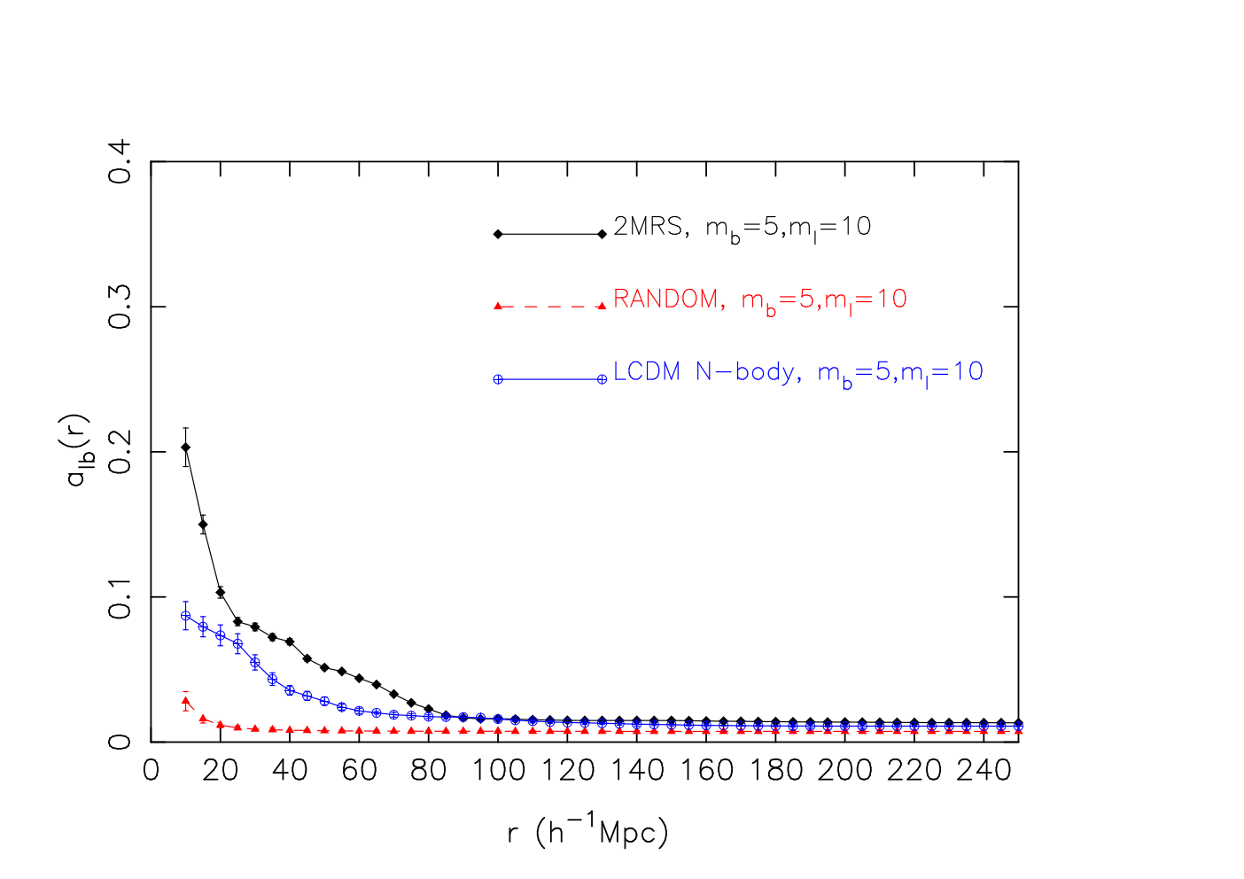
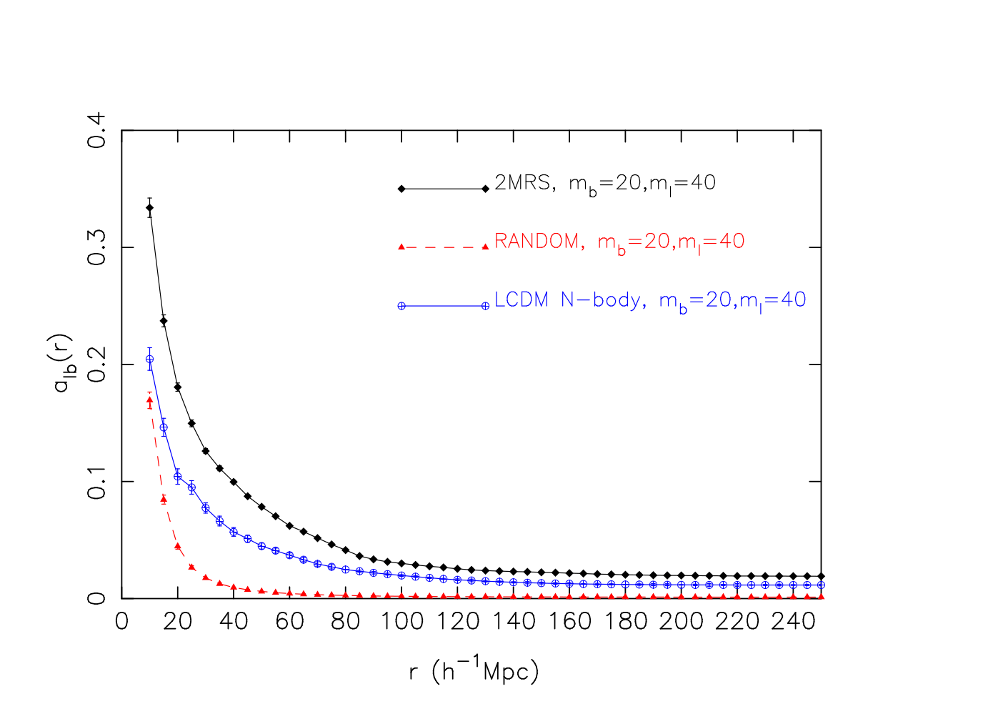
We show the degree of radial anisotropy as a function of length scales for the 2MRS sample and the mock samples from Poisson random distributions and N-body simulations of the CDM model in the top two panels of Figure 3. The choice of the number of bins are indicated in each panel. The error bars for the 2MRS galaxies are obtained from jackknife samples. The error bars for the random data and N-body data are obtained from the respective mock samples. The top left panel shows the results for and . This divides the entire sky into patches with exactly identical area. We see that the radial anisotropy in the 2MRS is maximum at the smallest radius considered. At the radius of the galaxy distribution is highly anisotropic and the level of anisotropy is much larger than that observed in the mock random samples. The mock random samples are isotropic by construction and the small anisotropies observed in the random samples are purely an outcome of the shot noise. It is interesting to note that the degree of the radial anisotropy in the 2MRS galaxy distribution decreases with increasing length scales and it reaches a plateau at where it is consistent with the level of anisotropies expected in a Poisson random distribution. In the top right panel we show the same results but for a different choice of the number of bins. Here we choose and i.e. the entire sky is now divided into equal area patches resulting into that many radial volume elements. Expectedly the level of anisotropies shoot up at small scale in both the 2MRS and random samples due to increase in the shot noise. The contribution of shot noise to the observed anisotropy is expected to dominate on small scales and it becomes negligible on large scales. We see the same trend for the 2MRS galaxies in the top right panel where the observed anisotropy decreases with increasing length scales and reaches a plateau at . However the differences in the degree of anisotropies in the 2MRS and the random samples increase when larger number of bins are used.
The present day galaxy distribution is highly anisotropic on small scales and the observed anisotropies originate from gravitational clustering, redshift space distortions (Kaiser, 1987), shot noise and the selection effects. We maintain the same shot noise and selection function in the random samples and the 2MRS sample. So the differences in the anisotropies in the galaxy distribution and the random samples are primarily due to the clustering of galaxies and the redshift space distortions.
The galaxies are distributed in the filamentary cosmic web. The galaxy clusters are usually located at the nodes where the filaments intersect. The virialized bound structures such as galaxy clusters are elongated along the line of sight in redshift space due to the random velocity dispersions which is popularly known as Fingers of God (FOG) effect. The individual volume elements are larger when a smaller number of pixels are used. Consequently they are expected to host a statistically similar number of these structures given the isotropy of the matter distribution. The increase in the number of bins corresponds to a decrease in the transverse dimension of the volume elements leading to a decrease in their volumes for a given radial extension. This makes it less likely to have a statistically similar number of FOGs in the different volume elements. But eventually this would happen at a large radius where the volume of the individual elements becomes significantly larger. So these differences in the anisotropies between the galaxy distribution and the Poisson distribution are the outcome of non-linear gravitational clustering on that angular scales. Despite these differences, the similarity in the results in the top two panels of the Figure 3 suggest that the galaxy distribution in the 2MRS become isotropic on length scales beyond .
We also compare the radial anisotropy expected in the CDM model to that observed in the 2MRS in the top two panels of Figure 3. We see that the mock catalogues from the CDM N-Body simulations exhibit a lower degree of anisotropy as compared to the 2MRS galaxies. This indicates that the 2MRS galaxies in the band are a biased tracer of the underlying mass distribution. A biased distribution is expected to be more anisotropic as compared to an unbiased distribution due to their differences in clustering. Using the magnitude of the clustering dipole Maller et al. (2003) find that the 2MASS galaxies in the band have a linear bias of . A further analysis of cosmological large scale flows (Davis et al., 2011) also suggest that the 2MRS galaxies have a linear bias of . So the differences in the degree of anisotropy in our analysis is most likely related to the fact that the 2MRS galaxies in the band are not an unbiased tracer of the mass distribution. However it is interesting to note that despite the differences in the degree of anisotropy between the galaxy distribution in 2MRS and CDM model, both the distributions become isotropic beyond a length scales of . We shall address the dependence of anisotropy on the clustering bias and explore the possibility of determining the linear bias from it in a separate work (in preparation).
The present analysis uses a tiling strategy which provides equal area pixelization of the sky but the pixel shapes may be quite different around the poles and the equator. This may have an important effect in the measured anisotropy. To examine this further, we use the HEALPix software (Górski et al., 1999; Górski et al., 2005) to calculate the radial anisotropy in the 2MRS data as function of and compare them with the measurements from our method. The left and right middle panels of Figure 3 compares the measurements from HEALPix and our scheme. In HEALPix we have used (NSide NPixels) and (NSide NPixels) to compare the results with that from our method for and respectively. We find that the measured anisotropies by HEALPix and our scheme show some differences when a small number of pixels are used. But interestingly they provide nearly identical results when the number of pixels are increased. This is most possibly related to the fact that the transverse dimensions of the volume elements become negligible as compared to their radial dimensions when a larger number of pixels are used. The statistics employed in this work use the number counts in the different volume elements integrated along the radial direction. So the disparity between the shape of the pixels becomes less important as compared their volumes when the number of pixels are increased. On the other hand, the differences between the radial and transverse dimensions of the volume elements are smaller when a smaller number of pixels are used and consequently the variations in their shapes may affect the anisotropy measurements. We also compute the radial anisotropy using only the galaxies outside the ZOA and compare it with the results obtained from the full sky analysis. We use HEALPix to analyze the unmasked regions of the sky using NSide NPixels and find that the measured anisotropies are exactly identical in both the cases. The comparison is shown in the middle right panel of Figure 3. This indicates that the anisotropy measure employed here is quite robust against incomplete sky coverage and reliably captures the anisotropic character of the distribution.
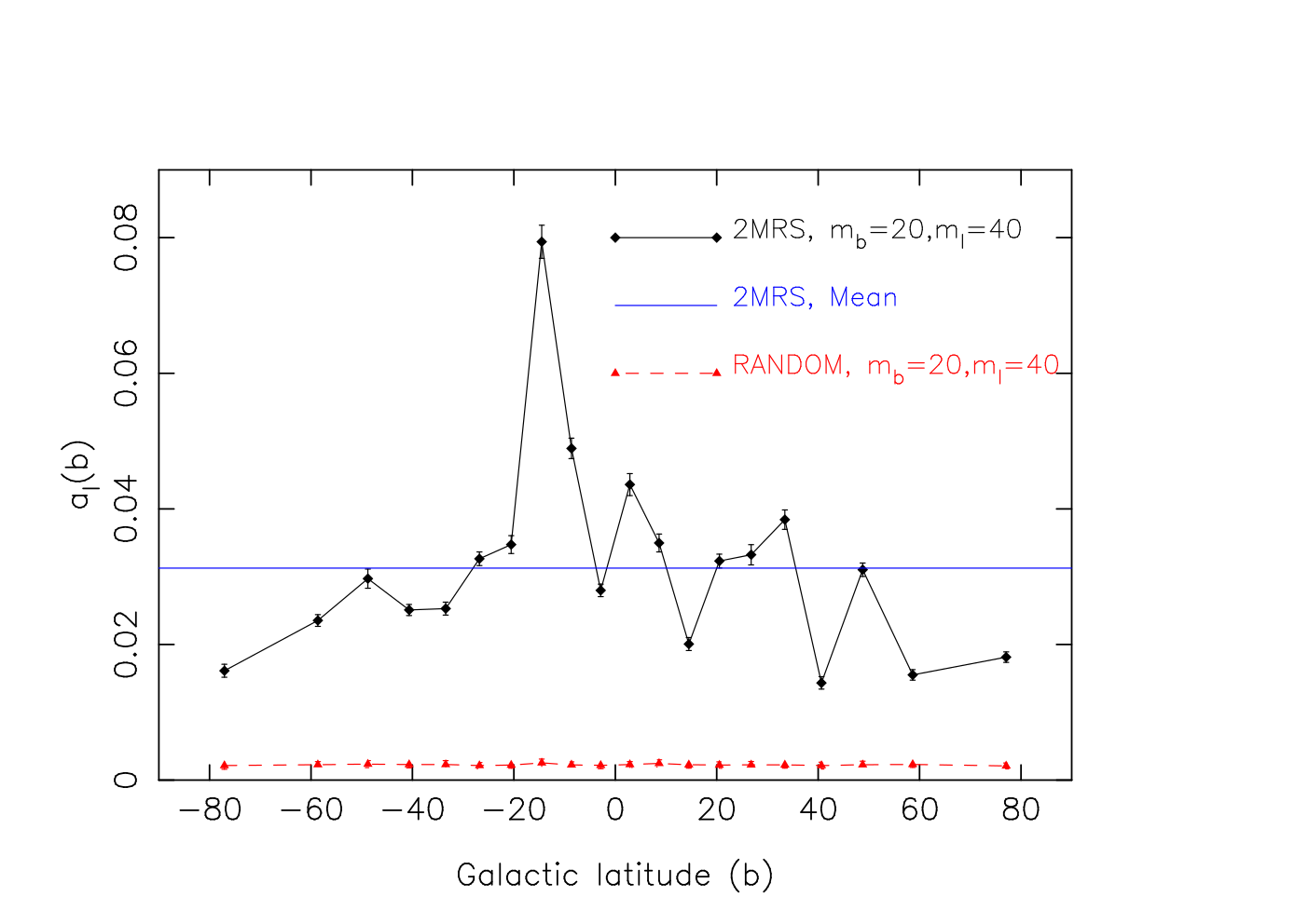
We show the polar anisotropy as a function of the galactic latitudes for the 2MRS galaxy sample and the mock random samples in the bottom left panel of Figure 3. We use and for this analysis. Both the 2MRS and the random samples exhibit a small degree of polar anisotropy. However the degree of polar anisotropy in the 2MRS galaxy distribution is noticeably higher as compared to the random samples. The anisotropy curve for the 2MRS galaxies is also spiky and irregular due to the anisotropies present in the galaxy distribution. The mean polar anisotropy for the 2MRS galaxies is also shown in the same plot. We see a distinct spike in the polar anisotropy curve for the 2MRS galaxies at where the polar anisotropy is of its mean value.
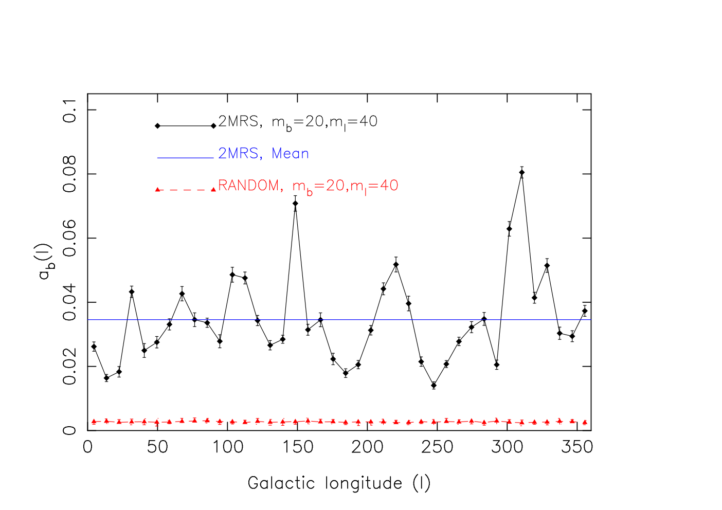
The azimuthal anisotropy as a function of galactic longitude for the 2MRS galaxy sample and the mock random samples are shown in the bottom right panel of Figure 3. The number of bins used in the analysis are and . We find a small degree of azimuthal anisotropy in both the 2MRS and the random samples. The degree of azimuthal anisotropy in the random samples are smaller than the 2MRS galaxy sample. The anisotropy curve for the random sample appears much smoother than the 2MRS galaxy sample. The random samples are isotropic by construction and the smaller amount of anisotropies observed in them arise purely due to the discreteness noise. On the other hand, the galaxy distribution is anisotropic due to the presence of large scale structures. This accounts for the relatively higher degree of anisotropy and the irregular nature of the anisotropy curve in the 2MRS sample compared to the mock random samples. The mean azimuthal anisotropy in the 2MRS sample is also shown together in the same plot. We find two distinct spikes in the azimuthal anisotropy curve, one at and another at where the anisotropies are and of the mean azimuthal anisotropies in the 2MRS.
We repeat the analysis with somewhat larger number of bins and find that the spikes in the two bottom panels of Figure 3 appear roughly at the same locations irrespective of the choice of the number of bins. But the results become shot noise dominated when a very large number of bins are used. The observed spikes in the anisotropy curves are most likely produced by some prominent large scale structures in the nearby Universe. One can see two visibly distinct structures at and in the top two panels of Figure 2. It is interesting to note that the distinct spikes in the anisotropies in the bottom two panels of Figure 3 appear at the same locations. Although it is difficult to reliably distinguish the large scale structures in projection, it is still interesting to note further that the two other smaller spikes which appears at and in the bottom right panel of Figure 3 correspond to two apparently underdense regions at those locations in the top right panel of Figure 2.
The Doppler effect due to the relative motion between the earth and the CMB rest frame is known to introduce a dipole anisotropy in the temperature of the CMB. The motion of the Local Group containing our galaxy is caused by the large scale structures in its neighbourhood. Analysis of the COBE DMR and PLANCK data suggest that the Local Group is moving with a velocity toward whereas the CMB dipole anisotropy is observed towards (Kogut et al., 1993; Planck Collaboration et al., 2014b). The misalignment of the CMB dipole with the clustering dipole and its convergence has been addressed in many studies (Yahil et al., 1980; Lynden-Bell et al., 1989; Rowan-Robinson et al., 2000; Erdoǧdu & Lahav, 2009; Lavaux et al., 2010; Bilicki et al., 2011). There is still no consensus on this issue mainly due to the sparseness of data at very large distances.
Clearly, the spikes observed in the two bottom panels of Figure 3 are not in the same direction as the CMB dipole or the clustering dipole. It is interesting to note that the two spikes in the azimuthal anisotropy are separated by i.e. they lie roughly in two opposite sides of the cone. The small value of combined with the fact that the two most anisotropic directions lie opposite each other in indicates a possible alignment of the Local Group with two nearby large scale structures. The radial anisotropy cease to exist beyond which imply that these large scale structures must lie within this radius. We verify this by changing from to and repeating the analysis. We again find the two prominent spikes in the anisotropy curves at the same locations as noticed earlier. It may be noted that some earlier studies with observed data (Peebles et al., 2001; Zitrin & Brosch, 2008) and simulations (Klypin et al., 2003) reported that the Local Group may reside in a filament. It has been also suggested by some studies (Tully et al., 2008; McCall, 2014) that the Local Group is a part of the Local Sheet which surrounds the Local Void (Tully & Fischer, 1987). It is interesting to note that using 2MASS photometric redshift measurements, Kovács & García-Bellido (2016) reported a significant antipodal anisotropy in the direction of the CMB cold spot . They find that the Eridanus supervoid reaches our closest vicinity in the directions of the CMB Cold Spot and continues to the nearby antipodal directions traversing upto the Northern Local Supervoid beyond which the antipodal line of sight becomes overdense due to the presence of Hercules and Corona Borealis superclusters.
Our analysis indicates that the nearby universe is highly anisotropic. The observed anisotropy gradually decreases with increasing radial distance and the galaxy distribution in the 2MASS redshift survey becomes statistically isotropic beyond a length scales of . In this study we have used the flux limited 2MRS sample and tested the isotropy of the Universe only around us. In future we plan to use the 2MASS photometric redshift catalogue (Bilicki et al., 2014) to construct volume limited samples for our study which will enable us to address the isotropy around different galaxies in the Universe. While searching for anisotropy in the polar and azimuthal directions, we identify two directions and which are significantly anisotropic compared to the other directions in the sky. Their preferential orientations may indicate a possible alignment of the Local Group with two nearby large scale structures. If so, the Milky way and the Local Group may be part of an extended filament in the cosmic web. However, it may be noted that the location of these anisotropy spikes may have some uncertainty due to their proximity to the zone of avoidance which is artificially filled by mirroring galaxies from the unmasked regions.
Pandey & Sarkar (2015) applied an information theory based method (Pandey, 2013) to the SDSS Main galaxy sample and find that the galaxy distribution in the Main sample is homogeneous on a scale of . The tests of isotropy in the present analysis is also based on the information theory. Our analysis indicates that besides the highly anisotropic nature of the present day galaxy distribution on small scales, the Universe is isotropic around us on scales beyond . This reaffirms the validity of the assumption of statistical isotropy on large scales and strengthens the foundations of the standard cosmological model.
5 ACKNOWLEDGEMENT
The author thanks an anonymous reviewer for the valuable comments and suggestions. The author thanks the 2MRS team for making the data public. The author also thanks Rishi Khatri for his help in using HEALPix. B.P. would like to acknowledge financial support from the SERB, DST, Government of India through the project EMR/2015/001037. B.P. would also like to acknowledge IUCAA, Pune and CTS, IIT, Kharagpur for providing support through associateship and visitors programme respectively.
References
- Akrami et al. (2014) Akrami, Y., Fantaye, Y., Shafieloo, A., et al. 2014, ApJ Letters, 784, L42
- Alonso et al. (2015) Alonso, D., Salvador, A. I., Sánchez, F. J., et al. 2015, MNRAS, 449, 670
- Appleby & Shafieloo (2014) Appleby, S., & Shafieloo, A. 2014, JCAP, 10, 070
- Barrow & Hervik (2010) Barrow, J. D., & Hervik, S. 2010, Physical Review D, 81, 023513
- Bengaly et al. (2015) Bengaly, C. A. P., Jr., Bernui, A., & Alcaniz, J. S. 2015, ApJ, 808, 39
- Bilicki et al. (2011) Bilicki, M., Chodorowski, M., Jarrett, T., & Mamon, G. A. 2011, ApJ, 741, 31
- Bilicki et al. (2014) Bilicki, M., Jarrett, T. H., Peacock, J. A., Cluver, M. E., & Steward, L. 2014, ApJS, 210, 9
- Blake & Wall (2002) Blake, C., & Wall, J. 2002, Nature, 416, 150
- Branchini et al. (2012) Branchini, E., Davis, M., & Nusser, A. 2012, MNRAS, 424, 472
- Briggs et al. (1996) Briggs, M. S., Paciesas, W. S., Pendleton, G. N., et al. 1996, ApJ, 459, 40
- Campanelli et al. (2011) Campanelli, L., Cea, P., Fogli, G. L., & Marrone, A. 2011, Physical Review D, 83, 103503
- Colles et al. (2001) Colles, M. et al.(for 2dFGRS team) 2001,MNRAS,328,1039
- Dai et al. (2013) Dai, L., Jeong, D., Kamionkowski, M., & Chluba, J. 2013, Physical Review D, 87, 123005
- Davis et al. (2011) Davis, M., Nusser, A., Masters, K. L., et al. 2011, MNRAS, 413, 2906
- Erdoǧdu et al. (2006b) Erdoǧdu, P., Lahav, O., Huchra, J. P., et al. 2006, MNRAS, 373, 45
- Erdoǧdu et al. (2006a) Erdoǧdu, P., Huchra, J. P., Lahav, O., et al. 2006, MNRAS, 368, 1515
- Erdoǧdu & Lahav (2009) Erdoǧdu, P., & Lahav, O. 2009, Physical Review D, 80, 043005
- Eriksen et al. (2007) Eriksen, H. K., Banday, A. J., Górski, K. M., Hansen, F. K., & Lilje, P. B. 2007, ApJ Letters, 660, L81
- Fixsen et al. (1996) Fixsen, D. J., Cheng, E. S., Gales, J. M., et al. 1996, ApJ, 473, 576
- Górski et al. (1999) Gorski, K. M., Wandelt, B. D., Hansen, F. K., Hivon, E., & Banday, A. J. 1999, arXiv:astro-ph/9905275
- Górski et al. (2005) Górski, K. M., Hivon, E., Banday, A. J., et al. 2005, ApJ, 622, 759
- Gruppuso et al. (2013) Gruppuso, A., Natoli, P., Paci, F., et al. 2013, JCAP, 7, 047
- Gupta & Saini (2010) Gupta, S., & Saini, T. D. 2010, MNRAS, 407, 651
- Hanson & Lewis (2009) Hanson, D., & Lewis, A. 2009, Physical Review D, 80, 063004
- Hazra & Shafieloo (2015) Hazra, D. K., & Shafieloo, A. 2015, JCAP, 11, 012
- Hoftuft et al. (2009) Hoftuft, J., Eriksen, H. K., Banday, A. J., et al. 2009, ApJ, 699, 985
- Huterer et al. (2015) Huterer, D., Shafer, D. L., & Schmidt, F. 2015, JCAP, 12, 033
- Huchra et al. (2012) Huchra, J. P., Macri, L. M., Masters, K. L., et al. 2012, ApJS, 199, 26
- Jackson (2012) Jackson, J. C. 2012, MNRAS, 426, 779
- Javanmardi et al. (2015) Javanmardi, B., Porciani, C., Kroupa, P., & Pflamm-Altenburg, J. 2015, ApJ, 810, 47
- Kaiser (1987) Kaiser, N. 1987, MNRAS, 227, 1
- Kalus et al. (2013) Kalus, B., Schwarz, D. J., Seikel, M., & Wiegand, A. 2013, A&A, 553, A56
- Kashlinsky et al. (2008) Kashlinsky, A., Atrio-Barandela, F., Kocevski, D., & Ebeling, H. 2008, ApJ Letters, 686, L49
- Kashlinsky et al. (2010) Kashlinsky, A., Atrio-Barandela, F., Ebeling, H., Edge, A., & Kocevski, D. 2010, ApJ Letters, 712, L81
- Kochanek et al. (2001) Kochanek, C. S., Pahre, M. A., Falco, E. E., et al. 2001, ApJ, 560, 566
- Kogut et al. (1993) Kogut, A., Lineweaver, C., Smoot, G. F., et al. 1993, ApJ, 419, 1
- Kovács & García-Bellido (2016) Ková cs, A., & García-Bellido, J. 2016, MNRAS, 462, 1882
- Klypin et al. (2003) Klypin, A., Hoffman, Y., Kravtsov, A. V., & Gottlöber, S. 2003, ApJ, 596, 19
- Land & Magueijo (2005) Land, K., & Magueijo, J 2005, Physical Review Letters, 95, 071301
- Lavaux et al. (2010) Lavaux, G., Tully, R. B., Mohayaee, R., & Colombi, S. 2010, ApJ, 709, 483
- Lin et al. (2016) Lin, H.-N., Wang, S., Chang, Z., & Li, X. 2016, MNRAS, 456, 1881
- Lynden-Bell et al. (1989) Lynden-Bell, D., Lahav, O., & Burstein, D. 1989, MNRAS, 241, 325
- Maller et al. (2003) Maller, A. H., McIntosh, D. H., Katz, N., & Weinberg, M. D. 2003, ApJ Letters, 598, L1
- Marinoni et al. (2012) Marinoni, C., Bel, J., & Buzzi, A. 2012, JCAP, 10, 036
- Marozzi & Uzan (2012) Marozzi, G., & Uzan, J.-P. 2012, Physical Review D, 86, 063528
- McCall (2014) McCall, M. L. 2014, MNRAS, 440, 405
- Meegan et al. (1992) Meegan, C. A., Fishman, G. J., Wilson, R. B., et al. 1992, Nature, 355, 143
- Moss et al. (2011) Moss, A., Scott, D., Zibin, J. P., & Battye, R. 2011, Physical Review D, 84, 023014
- Rowan-Robinson et al. (2000) Rowan-Robinson, M., Sharpe, J., Oliver, S. J., et al. 2000, MNRAS, 314, 375
- Pandey (2013) Pandey, B. 2013, MNRAS, 430, 3376
- Pandey (2016) Pandey, B. 2016, MNRAS, 462, 1630
- Pandey (2016) Pandey, B. 2016, MNRAS, 463, 4239
- Pandey & Sarkar (2015) Pandey, B., & Sarkar, S. 2015, MNRAS, 454, 2647
- Peebles et al. (2001) Peebles, P. J. E., Phelps, S. D., Shaya, E. J., & Tully, R. B. 2001, ApJ, 554, 104
- Penzias & Wilson (1965) Penzias, A. A., & Wilson, R. W. 1965, ApJ, 142, 419
- Planck Collaboration et al. (2014b) Planck Collaboration, Aghanim, N., Armitage-Caplan, C., et al. 2014, A&A, 571, A27
- Planck Collaboration et al. (2014a) Planck Collaboration, Ade, P. A. R., Aghanim, N., et al. 2014, A&A, 571, A23
- Planck Collaboration et al. (2016b) Planck Collaboration, Ade, P. A. R., Aghanim, N., et al. 2016, A&A, 594, A16
- Planck Collaboration et al. (2016a) Planck Collaboration, Ade, P. A. R., Aghanim, N., et al. 2016, A&A, 594, A13
- Schwarz et al. (2004) Schwarz, D. J., Starkman, G. D., Huterer, D., & Copi, C. J. 2004, Physical Review Letters, 93, 221301
- Schwarz & Weinhorst (2007) Schwarz, D. J., & Weinhorst, B. 2007, A&A, 474, 717
- Shannon (1948) Shannon, C. E. 1948, Bell System Technical Journal, 27, 379-423, 623-656
- Scharf et al. (2000) Scharf, C. A., Jahoda, K., Treyer, M., et al. 2000, ApJ, 544, 49
- Smoot et al. (1992) Smoot, G. F., Bennett, C. L., Kogut, A., et al. 1992, ApJ Letters, 396, L1
- Soda (2012) Soda, J. 2012, Classical and Quantum Gravity, 29, 083001
- Tully et al. (2008) Tully, R. B., Shaya, E. J., Karachentsev, I. D., et al. 2008, ApJ, 676, 184-205
- Tully & Fischer (1987) Tully, R. B. & Fischer, J. R. 1987, Nearby Galaxies Atlas, Cambridge University Press
- Watkins et al. (2009) Watkins, R., Feldman, H. A., & Hudson, M. J. 2009, MNRAS, 392, 743
- Wilson & Penzias (1967) Wilson, R. W., & Penzias, A. A. 1967, Science, 156, 1100
- Wu et al. (1999) Wu, K. K. S., Lahav, O., & Rees, M. J. 1999, Nature, 397, 225
- Yahil et al. (1980) Yahil, A., Sandage, A., & Tammann, G. A. 1980, ApJ, 242, 448
- York et al. (2000) York, D. G., et al. 2000, AJ, 120, 1579
- Zitrin & Brosch (2008) Zitrin, A., & Brosch, N. 2008, MNRAS, 390, 408