On the Security of Warning Message Dissemination in Vehicular Ad Hoc Networks
Abstract
Information security is an important issue in vehicular networks as the accuracy and integrity of information is a prerequisite to satisfactory performance of almost all vehicular network applications. In this paper, we study the information security of a vehicular ad hoc network whose message may be tampered by malicious vehicles. An analytical framework is developed to analyze the process of message dissemination in a vehicular network with malicious vehicles randomly distributed in the network. The probability that a destination vehicle at a fixed distance away can receive the message correctly from the source vehicle is obtained. Simulations are conducted to validate the accuracy of the theoretical analysis. Our results demonstrate the impact of network topology and the distribution of malicious vehicles on the correct delivery of a message in vehicular ad hoc networks, and may provide insight on the design of security mechanisms to improve the security of message dissemination in vehicular networks.
Index Terms:
Vehicular ad hoc networks, message dissemination, security.I Introduction
Interest is surging on vehicular networks and Internet-of-vehicles technologies due to their increasingly important role in improving road traffic efficiency, enhancing road safety and providing real-time information to drivers and passengers [1]. By deploying wireless communication infrastructure along the roadside (e.g., road-side units (RSU)), equipping vehicles with on-board communication facilities (e.g., on-board units (OBU)), and with the assistance of dedicated short-range communication (DSRC) [2] and LTE technology, two wireless communication modes: vehicle-to-infrastructure and vehicle-to-vehicle communications, are supported in vehicular networks. Through wireless communications, messages can be disseminated for vehicular network applications, including safety applications requiring real-time information about traffic accidents, traffic congestion or obstacles in the road, and non-safety applications such as offering value-added services (e.g., digital maps with real-time traffic status) and in-car entertainment services [3].
Coming together with the convenience and advantage of wireless communications is the potential security threat that vehicular networks may present to transportation systems. Different from traditional security settings, in vehicular networks, information collection and dissemination are conducted by distributed vehicles. Quite often, information may be generated by or received from a vehicle that has never been encountered before. This may render traditional security mechanisms, largely based on cryptography and key management, or trust management, futile in vehicular networks. The situation is further exacerbated by the highly dynamic topology of vehicular networks where the connections may emerge opportunistically between vehicles and the associated network topology is constantly changing [4]. All these features of vehicular networks pose unique challenges for vehicular network security and make vehicular networks prone to attacks by malicious and/or selfish attackers who may spread false messages, tamper or drop the received messages. These security threats are likely to result in severe consequences like traffic congestion, traffic crash, even loss of lives and must be thoroughly investigated before vehicular networks can be deployed.
In this paper, we study information security of vehicular ad hoc networks (VANETs), where the message may be tampered by malicious vehicles randomly distributed in the network, by investigating the probability that a destination vehicle at a fixed distance away can receive the message correctly from the source vehicle. Specifically, consider that a vehicle (i.e., the source vehicle) detecting an abnormal situation, e.g., traffic accident, slippery road and congestion, sends a message informing other vehicles of the situation. The message is forwarded from the source vehicle in a multi-hop manner to other vehicles. We analyze the probability that a vehicle at a fixed distance away, termed the destination vehicle, can receive the message correctly from the source vehicle in the presence of malicious vehicles in between, which may modify the transmitted message. The novelty and major contributions of this paper are summarized as follows:
- 1.
We develop for the first time an analytical framework to model the process of message dissemination in vehicular ad hoc networks in the presence of malicious vehicles randomly distributed in the network. The probability that a message is delivered correctly from the source vehicle to a destination vehicle at a fixed distance away is analyzed.
- 2.
Simulations are conducted to establish the accuracy of the analysis. Using the analysis, relationship is revealed between key parameters such as the probability of correct message reception and its major performance-impacting parameters. Discussions are presented on the impact of network topology and the distribution of malicious vehicles on secure message delivery in vehicular networks.
- 3.
Our results may provide insight on the design of security mechanisms, particularly secure routing algorithms and topology control algorithms, to improve informations security in vehicular networks.
The rest of this paper is organized as follows: Section II reviews related work. Section III introduces the system model and the problem formation. Theoretical analysis is presented in Section IV. In Section V, we conduct simulations to validate the accuracy of our analysis and discuss its insight. Section VI concludes this paper.
II Related Work
For secure message dissemination in vehicular networks, two major factors need to be considered: the trustworthiness of each vehicle and the integrity of the transmitted message. Accordingly, three misbehavior detection schemes are commonly adopted for secure message dissemination: entity-centric misbehavior detection scheme, data-centric misbehavior detection scheme, and a combined use of both. In the following, we will review the works on these three schemes separately.
Entity-centric misbehavior detection schemes focus on assessing the trustworthiness level of each vehicle to filter out the malicious vehicles. The assessment process is commonly conducted at each vehicle by monitoring their instantaneous neighbors’ behavior. In [5], Gazdar et al. proposed a dynamic and distributed trust model to formalize a trust relationship between vehicles and filter out malicious and selfish vehicles. Their trust model is based on the use of a Markov chain to evaluate the evolution of the trust value. In [6], instead of allowing all vehicles to assess trustworthiness, Khan et al. proposed a novel malicious node detection algorithm for VANETs, which optimizes the selection of assessors to improve the overall network performance. In [7], Haddadou et al. proposed a distributed trust model for VANETs, which was motivated by the job market signaling model. Their trust model is able to gradually detect all malicious nodes as well as boosting the cooperation of selfish nodes. In [8], to overcome the challenges of intermittent and ad hoc monitoring and assessment processes caused by the high mobility and rapid topology change in vehicular networks, Sedjelmaci et al. proposed a lightweight intrusion detection framework with the help of a clustering algorithm, where nodes are grouped into highly stable clusters so that the monitoring and assessment processes can be better conducted in a relatively stable environment.
Data-centric misbehavior detection schemes focus on the consistency check of the disseminated data to filter out the false data. In [9], Dietzel et al. argued that redundant data forwarding paths are the most promising technique for effective data consistency check in a multi-hop information dissemination environment, and proposed three graph-theoretic metrics to measure the redundancy of dissemination protocols. In [10], Raya et al. proposed a framework for vehicular networks to establish data-centric trust, and evaluated the effectiveness of four data fusion rules: majority voting, weighted voting, Bayesian inference and belief propagation based techniques. In [11], Huang et al. firstly demonstrated that information cascading and oversampling adversely affect the performance of trust management scheme in VANETs, and then proposed a novel voting scheme that taking the distance between the transmitter and receiver into account when assigning weight to the trust level of the received data. In [12], Zaidi et al. proposed and evaluated a rogue node detection system for VANETs using statistical techniques to determine whether the received data are false. In [13], Radak applied a so-called cautious operator to deal with data received from different sources to detect dangerous events on the road. Their adopted cautious operator is an extension of the Demper-Shafer theory that is known to be superior in handling data come from dependent sources.
A combined use of entity-centric and data-centric misbehavior detection scheme makes use of both the trust level of vehicles and the consistency of received data to detect misbehaving vehicles and filter out incorrect messages. Works adopting the combined scheme are limited. In [14], Dhurandher proposed a security algorithm using both node reputation and data plausibility checks to protect the network against attacks. The reputation value is obtained by both direct monitoring and indirect recommendation from neighbors; and the data consistency check is conducted by comparing the received data with the sensed data by the vehicle’s own sensors. In [15], Li et al. proposed an attack-resistant trust management scheme to evaluate the trustworthiness of both data and vehicles in VANETs, and to detect and cope with malicious attacks. They adopted the Dempster-Shafer theory to combine the data received from different sources, and then used this combined result to update the trust value of vehicles.
In summary, all the above works on security issues in vehicular networks focused on trust model establishment, trust model management, or methods to assess data from different sources to check their consistency, with a goal of detecting misbehaving nodes in the network. Our work is different from theirs in that we focus on theoretically characterizing the probability of correct message reception, and evaluate the impact of network topology and distribution of malicious vehicles on the probability.
III System Model and Problem Formation
III-A Network Model
We consider a vehicular ad hoc network on a highway with bi-directional traffic flows. Vehicles in both directions are distributed randomly following Poisson point processes [16, 17] with spatial densities and respectively. As a ready consequence of the superposition property of Poisson processes [18], all vehicles on the highway are also Poissonly distributed with density . In actual road networks, there may be multiple lanes in each direction. Considering that the width of a lane is typically small compared with the transmission range of vehicles, we ignore the road width and model multiple lanes in the same direction as one lane [16, 19].
III-B Wireless Communication Model
We consider a general wireless connection model [20], where a receiver separated by a Euclidean distance from a transmitter receives the message successfully with a probability , independent of transmissions by other transmitter-receiver pairs. There are two constraints on : 1) it is a monotonic non-increasing function of and 2) . This general wireless connection model includes a number of widely-used wireless connection models as its special cases. For instance, when assumes the following form
| (1) |
it becomes the widely known unit disk model where a pair of wireless nodes are directly connected when their Euclidean distance is smaller than or equal to a threshold , known as the transmission range. Alternatively, when takes the following form,
| (2) |
it becomes another widely known log-normal connection model [21, 22, 23], where is the path loss exponent, is the standard deviation and is the equivalent transmission range when .
We consider a network with a sufficiently large vehicular density such that the generated vehicular network is a connected network [21]. Besides, broadcast transmission is adopted so that each message can be received by multiple vehicles to increase the number of redundant data forwarding paths and reduce the message dissemination time. Furthermore, we assume that time is divided into time slots of equal length and is sufficiently small such that we can regard vehicles as almost stationary during each time slot. After the message dissemination process begins, at each time slot, a vehicle among the set of vehicles that 1) have received at least one message and 2) are yet to transmit the message, is randomly chosen to broadcast its received message. Such broadcast protocol can be readily implemented in a distributed manner by having each vehicle waits a random amount of time identically and independently distributed following an exponential distribution before transmitting its received message. Each vehicle only transmits its received message once. Note that the radio propagation speed is much faster than the moving speed of vehicles [24]. Therefore, we ignore the information propagation delay in this paper and assume that during the message dissemination process, the topology of the vehicular network remains unchanged.
III-C Malicious Vehicle distribution and Data Fusion Rule
We assume that vehicles along the highway can be classified into two categories: normal vehicles, which behave normally and will forward the received message without any alteration, and malicious vehicles, which may tamper the received message and alter its content. Beside, we assume that the probability of each vehicle being a malicious vehicle is , independent of the event that another distinct vehicle is a malicious vehicle. We further assume that the malicious vehicles act in a distributed manner and there is no central coordination among malicious vehicles. As a consequence of the assumption, each malicious vehicle simply modifies the received message without evaluation of the true content of the message.
Following the broadcast dissemination scheme considered in the paper, each vehicle is likely to receive multiple copies of a message from different vehicles before it broadcasts the message. Due to the existence of malicious vehicles, the received messages may not be the same. For example, one vehicle may detect a traffic incident and generate a message alerting other vehicles but this message may be modified by a malicious vehicle. In the situation of conflicting messages being received, a majority voting rule is employed by each vehicle to fuse their received messages. That is, the normal vehicle will broadcast the message in agreement with the most number of vehicles and discard the message conflicting with majority opinion, and the malicious vehicle will broadcast the message conflicting with the majority opinion. When a tie occurs, all the vehicles will randomly choose one of the two messages (true or false message) with equal probability to broadcast. The simplicity of the majority voting rule allows us to focus on the topological impact of vehicular networks on the correct message delivery. It is part of our future work plan to investigate the optimum fusion rule for highly dynamic vehicular networks.
III-D Problem Formation
Given the aforementioned background, we are now ready to give a formal definition of the problem considered in this paper.
Consider a vehicle, termed the source vehicle , detects an accident in front of it and wants to deliver a warning message to vehicles traveling in the same direction as and behind in that direction. Designate the location of at the time instant when it broadcasts the message as the origin, and the direction of information propagation (in the opposite direction of the travel direction of ) as the positive direction. We want to investigate the probability that a vehicle, termed the destination vehicle , located at distance away from can receive the message of correctly. We denote by the sub-network we focus on, which is within the road segment , and with vehicular density and a wireless connection model . See Fig. 1 for an illustration.

Two kinds of messages are considered in this paper, represents the true message (e.g., road is congested) and represents the false message (e.g., road is not congested). Here we assume that the source vehicle is a normal vehicle, namely, the message broadcast by the source vehicle is true. For malicious vehicles, as there are no central coordination among them, there is no way for a malicious vehicle to know the true content of the message. Therefore, it is assumed that a malicious vehicle simply modify the content of whatever message it receives (against the outcome of the majority voting rule), i.e., changing to and to .
Finally, the destination vehicle conducts its majority voting process after it has received all messages, or equivalently after no further message is received after a long time period. Denote by the concluded message after has completed its data fusion. In this paper, we are interested in investigating the probability that the destination vehicle receives the correct message, denoted by , which can be expressed as follows:
| (3) |
IV Theoretical Analysis
In this section, we will present our analysis on the probability that the destination vehicle receives the message correctly.
From the definition of the probability of correct message reception, which is given in (3), can be expressed as follows as an easy consequence of the total probability theorem:
| (4) |
where denotes the random number of vehicles located in the sub-network . Due to the Poisson distribution of vehicles, we have
| (5) |
Recall that in our system, the source vehicle located at the origin broadcasts its message first. After that, at each time slot, a vehicle among the set of vehicles having received at least one message and having not broadcast its message is randomly chosen to broadcast. Denote by the th vehicle that broadcasts the message and denote its location by , where is a random variable representing the location of the th vehicle broadcasting its message. We designate the source vehicle as the th broadcast vehicle and its location is . It follows that the destination vehicle then becomes the th broadcast vehicle. Using the total probability theorem, the conditional probability that the destination vehicle receives the correct message (after its fusion), given there are vehicles located in the sub-network , can be calculated by
| (6) |
where is the joint distribution (probability density function) of the locations of the st, nd, , and th broadcast vehicles.
Combining (4) - (6), it can be shown that to obtain the correct message reception probability , it remains to calculate the conditional probability that the destination vehicle receives the message correctly given that the th broadcast vehicle is located at , i.e., , and the joint distribution of the locations of the st, nd, , and th broadcast vehicles, i.e., . In the following, we will calculate these two terms separately.
IV-A Calculation of
Denote by the indicator function that represents whether the destination vehicle receives the message sent by the th broadcast vehicle located at . Following the general wireless connection model considered in the paper, it can be readily shown that
| (7) |
Denote by the message broadcast by the th broadcast vehicle located at , . It follows that as we regard the source vehicle is a normal vehicle that broadcasts the true message, and each is a binary random variable taking value from . Assuming the majority voting rule, the conditional probability that the destination vehicle receives the message correctly given that the th broadcast vehicle is located at , , can be calculated by:
| (8) |
where the vector is defined by , and the first step follows from the rule of majority voting, particularly noting that when a tie occurs, the destination vehicle will make a decision randomly with equal probability. The second step is obtained by using the total probability theorem on . Note from (7) that each is a binary random variable. Therefore, the vector can have possible values and we let represents each possible value. The third step follows by plugging , which readily results from the definition of each given as (7).
From (8), to calculate , it remains to calculate the two terms and given each fixed , . Using the joint distribution of , , , the above two terms can be obtained as follows:
| (9) |
and
| (10) |
According to the chain rule of probability, it can be readily obtained that the joint distribution of , is given by
| (11) |
Note that the message fusion result of vehicle is dependent on the messages broadcast by vehicles . Therefore, the conditional distribution of each , given can be obtained as follows:
| (12) |
and
| (13) |
where the three terms in (12) are the probabilities that vehicle broadcasts message under three different cases: , , and separately. Using the first case as an example to illustrate: when , vehicle would conclude from its majority voting process that the majority opinion of the message is . Considering each vehicle has probability to modify the message (being a malicious vehicle), therefore, the probability for the vehicle to broadcast the correct concluded message (from the majority voting process) would be , which leads to the term . Specifically, from (12), when we have
| (14) |
and
| (15) |
which can also be readily obtained as the st broadcast vehicle only receives the true message from the source vehicle.
IV-B Calculation of
Let be the set of vehicles in the sub-network which have received at least one message after the th broadcast vehicle has broadcast its messages. Given the location of the th broadcast vehicle as , a vehicle located at belongs to implies that it connects to at least one vehicle that are located at , which has the probability . Note that the th broadcast vehicle is randomly chosen from the vehicle set , therefore, given each , the location of th broadcast vehicle has the conditional probability density function as follows:
| (16) |
Eq. (16) is valid when as we assume each vehicle only broadcasts once. Particularly, when , we have the probability density function of the st broadcast vehicle’s location
| (17) |
V Simulation and Discussion
In this section, numerical and simulation results are shown to discuss the relationship between the probability of correct message reception and its major performance-impacting parameters. Specifically, we adopt the unit disk model and the log-normal connection model as two special cases of the general wireless connection model respectively in the simulation. For the unit disk model, we set the transmission range m (typical radio range using DSRC [25]), and for the log-normal connection model, we set the the path loss exponent and the standard deviation [20]. Each simulation is repeated 5000 times and the average value is shown in the plot.
Fig. 2 shows a comparison between the analytical result and the simulation result assuming the unit disk model, and shows that the analytical result matches very well with the simulation result.

Fig. 3 and Fig. 4 show the relationship between the probability of correct message reception and the probability of each vehicle being malicious assuming the unit disk model, under different distance between the source vehicle and the destination vehicle, and under different vehicular density respectively. Specifically, we can see that when , which corresponds to the case that all vehicles are normal vehicles; when is small, decreases sharply with an increase of and decreases to its minimum value ( in our system) when is larger than a certain threshold , e.g., when km and veh/m. Beyond that threshold, a further increase in has little impact on . This can be explained by the fact that when , the number of malicious vehicles in the network is small. Therefore, an increase in will largely increase the number of malicious vehicles, which consequently, leads to a sharp decrease in the probability of correct message reception. When is larger than its threshold, malicious vehicles play dominant roles in the majority voting scheme. In this case, for any vehicle in the network, the outcome of its message fusion result will be incorrect. The minimum value of is due to the fact that malicious vehicles in our network simply modify the received message without evaluation of the true content of the message. Therefore, when is larger than its threshold, the message transmitted in the network will move between and back and forth, leading to the occurrence that converges to 0.5 instead of 0.


Fig. 3 shows that given a fixed vehicular density, when , a larger distance between the source vehicle and the destination vehicle will lead to a smaller . This is due to the fact that other things being equal, a larger implies a larger number of malicious vehicles participating in tampering the message transmitted from the source vehicle to the destination vehicle. As a consequence, it leads to a smaller .
Fig. 4 shows that in our system, a larger vehicular density has little impact on . Intuitively, a larger will lead to a larger due to the fact that a larger implies a larger number of messages received by each vehicle, which is beneficial for vehicles to conduct data consistency checks. Therefore, when the traffic density increases, the message fusion result of each vehicle will be more accurate. Consequently, other things being equal, the probability of correct message reception will increase. However, when a vehicle is randomly chosen among the set of vehicles that have received at least one message to broadcast, it may not have received a sufficient number messages from other vehicles to conduct a robust data fusion. This follows that even with an increase in traffic density , the message fusion result of each broadcast vehicle does not improve. Therefore, a larger vehicular density has little impact on the .
Fig. 5 and Fig. 6 show the relationship between the probability of correct message reception and the probability of each vehicle being malicious assuming the log-normal connection model, under different distance between the source vehicle and the destination vehicle, and under different vehicular density respectively. We can see that with the increase of from to , the trend of is the same as that assuming the unit disk model. Therefore, we omit the duplicate discussion here.
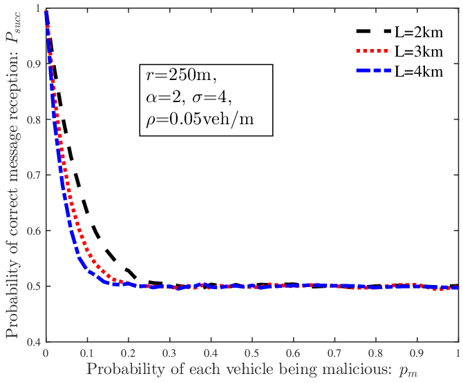

Fig. 7 gives a comparison of the correct message reception probability achieved assuming the unit disk model (labeled as UDM) and that achieved assuming the log-normal connection model (labeled as LSM). It is shown that when , the system assuming the log-normal connection model has a slightly higher correct message reception probability than that assuming the unit disk model. The reason behind this phenomenon is that the log-normal connection model introduces a Gaussian variation of the transmission range around the mean value, which implies a higher chance for the vehicles to be connected to other vehicles separated further away. Therefore, other things being equal, each broadcast vehicle assuming the log-normal connection model can receive more copies of a message from other vehicles than that assuming the unit disk model, which leads to a better message fusion result for each vehicle and consequently, results in a higher correct message reception probability.

VI Conclusions
This paper studied a vehicular ad hoc network where a certain fraction of vehicles are malicious vehicles and these malicious vehicles are distributed randomly in the network. Furthermore, there is no central coordination among these malicious vehicles and consequently a malicious vehicle simply modify its received message irrespective of its true value. An analytical framework is developed to model the process of secure message dissemination in the network, and the probability that a vehicle, located at a fixed distance away from the source vehicle, can receive the message correctly is obtained. Simulations were conducted to establish the accuracy of the analytical results and demonstrate that the probability of correct message delivery reduces to its minimum after the proportion of malicious vehicles in the network increases beyond a threshold. Besides, a smaller distance between the destination vehicle and the source vehicle will lead to a larger probability of correct message reception. Our results may provide insight on the design of security mechanisms, particularly secure routing algorithms and topology control algorithms, to enhance secure message dissemination in highly dynamic vehicular networks.
References
- [1] K. Zheng, et al., “Heterogeneous Vehicular Networking: A Survey on Architecture, Challenges, and Solutions,” IEEE Communication Survey & Tutorials, vol. 17, no. 4, pp. 2377-2396, Fourth Quarter, 2015.
- [2] J. B. Kenney, “Dedicated Short-Range Communications (DSRC) Standards in the United States,” Proceedings of the IEEE, vol. 99, no. 7, pp. 1162-1182, 2011.
- [3] S. Ilarri, T. Delot, R. Trillo-Lado, “A Data Management Perspective on Vehicular Networks,” IEEE Communication Survey & Tutorials, vol. 17, no. 4, pp. 2420-2460, Fourth Quarter, 2015.
- [4] G. Mao and B. D.O. Anderson, “Graph Theoretic Models and Tools for the Analysis of Dynamic Wireless Multihop Networks”, in IEEE WCNC, pp. 1-6, 2009.
- [5] T. Gazdar, A. Rachedi, A. Benslimane, and A. Belghith, “A distributed advanced analytical trust model for VANETs,” in IEEE Global Communications Conference (GLOBECOM) 2012.
- [6] U. Khan, S. Agrawal, and S. Silakari, “Detection of Malicious Nodes (DMN) in Vehicular Ad-Hoc Networks,” Procedia Computer Science, vol. 46, pp. 965-972, 2015.
- [7] N. Haddadou, A. Rachedi, and Y. Ghamri-Doudane, “A Job Market Signaling Scheme for Incentive and Trust Management in Vehicular Ad Hoc Networks,” IEEE Transactions on Vehicular Technology, vol. 64, no. 8, pp. 3657-3674, Aug. 2015.
- [8] H. Sedjelmaci, and S. M. Senouci, “An accurate and efficient collaborative intrusion detection framework to secure vehicular networks”, Computers and Electrical Engineering, vol. 43, pp. 33-47, 2015.
- [9] S. Dietzel, J. Petit, G. Heijenk, and F. Kargl, “Graph-Based Metrics for Insider Attack Detection in VANET Multihop Data Dissemination Protocols,” IEEE Transactions on Vehicular Technology, vol. 62, no. 4, pp. 1505-1518, May. 2013.
- [10] M. Raya, P. Papadimitratos, V. D. Gligor, and J. P. Hubaux, “On Data-Centric Trust Establishment in Ephemeral Ad Hoc Networks,” in IEEE INFOCOM 2008.
- [11] Z. Huang, S. Ruj, M. A. Cavenaghi, M. Stojmenovic, and A. Nayak, “A social network approach to trust management in VANETs,” Peer-to-Peer Networking and Applications, vol. 7, no. 3, pp. 229-242, 2014.
- [12] K. Zaidi, M. B. Milojevic, V. Rakocevic, A. Nallanathan, and M. Rajarajan, “Host-Based Intrusion Detection for VANETs: A Statistical Approach to Rogue Node Detection,” IEEE Transactions on Vehicular Technology, vol. 65, no. 8, pp. 6703-6714, Aug. 2014.
- [13] J. Radak, B. Ducourthial, V. Cherfaoui, and S. Bonnet, “Detecting Road Events Using Distributed Data Fusion: Experimental Evaluation for the Icy Roads Case,” IEEE Transactions on Intelligent Transportation Systems, vol. 17, no. 1, pp. 184-194, Jan. 2016.
- [14] S. K. Dhurandher, M. S. Obaidat, A. Jaiswal, A. Tiwari and A. Tyagi, “ Vehicular Security Through Reputation and Plausibility Checks,” IEEE system journal, vol. 8, no. 2, pp. 384 - 394. Jun. 2014.
- [15] W. Li, and H. Song, “ART: An Attack-Resistant Trust Management Scheme for Securing Vehicular Ad Hoc Networks,” IEEE Transactions on Intelligent Transportation Systems, vol. 17, no. 4, pp. 960-969, Apr. 2016.
- [16] N. Wisitpongphan, et al., “Routing in Sparse Vehicular Ad Hoc Wireless Networks,” IEEE Journal on Selected Areas in Communications, vol. 25, no. 8, pp. 1538-1556, Oct. 2007.
- [17] A. B. Reis, et al., “Deploying Roadside Units in Sparse Vehicular Networks: What Really Works and What Does Not,” IEEE Transactions on Vehicular Technology, vol. 63, no. 6, pp. 2794-2806, Jul. 2014.
- [18] R. Nelson, Probability, Stochastic Processes, and Queueing Theory: The Mathematics of Computer Performance Modeling. New York: Springer- Verlag, 1995.
- [19] K. Abboud and W. Zhuang, “Stochastic Analysis of a Single-Hop Communication Link in Vehicular Ad Hoc Networks,” IEEE Transactions on Intelligent Transportation Systems, vol. 15, no. 5, pp. 2297-2307, Oct. 2014.
- [20] Z. Zhang, G. Mao, T. Han and B. D. O. Anderson, “Cooperative Information Forwarding in Vehicular Networks Subject to Channel Randomness,” in Proceedings of IEEE ICC, 2014.
- [21] G. Mao, “Connectivity of Communication Networks”, Springer, ISBN 978-3-319-52989-9, March 2017.
- [22] G. Mao and B. D. O. Anderson, “Towards a Better Understanding of Large Scale Network Models”, IEEE/ACM Transactions on Networking, Vol. 20, No. 2, pp. 408 - 421, 2012.
- [23] G. Mao and B. D. O. Anderson, “Connectivity of Large Wireless Networks under a General Connection Model”, in IEEE Transactions on Information Theory, Vol. 59, No. 3, pp. 1761 - 1772, 2013.
- [24] Z. Zhang, G. Mao, and B. D. O. Anderson, “Stochastic Characterization of Information Propagation Process in Vehicular Ad hoc Networks,” IEEE Transactions on Intelligent Transportation Systems, vol. 15, no. 1, pp. 122-135, Feb. 2014.
- [25] Z. Haibo, L. Bo, T. H. Luan, H. Fen, G. Lin, L. Ying, Q. Yu, and X. Shen, “ChainCluster: Engineering a Cooperative Content Distribution Framework for Highway Vehicular Communications,” IEEE Transactions on Intelligent Transportation Systems, vol. 15, no.6, pp. 2644-2657, Dec. 2014.