Truth and Regret in Online Scheduling

Shuchi Chawla Affiliation: University of Wisconsin-Madison (shuchi@cs.wisc.edu) Nikhil Devanur Affiliation: Microsoft Research (nikdev@microsoft.com) Janardhan Kulkarni Affiliation: Microsoft Research (jakul@microsoft.com) Affiliation: Cornell University (rad@cs.cornell.edu) Rad Niazadeh

Abstract

We consider a scheduling problem where a cloud service provider has multiple units of a resource available over time. Selfish clients submit jobs, each with an arrival time, deadline, length, and value. The service provider’s goal is to implement a truthful online mechanism for scheduling jobs so as to maximize the social welfare of the schedule. Recent work shows that under a stochastic assumption on job arrivals, there is a single-parameter family of mechanisms that achieves near-optimal social welfare. We show that given any such family of near-optimal online mechanisms, there exists an online mechanism that in the worst case performs nearly as well as the best of the given mechanisms. Our mechanism is truthful whenever the mechanisms in the given family are truthful and prompt, and achieves optimal (within constant factors) regret.

We model the problem of competing against a family of online scheduling mechanisms as one of learning from expert advice. A primary challenge is that any scheduling decisions we make affect not only the payoff at the current step, but also the resource availability and payoffs in future steps. Furthermore, switching from one algorithm (a.k.a. expert) to another in an online fashion is challenging both because it requires synchronization with the state of the latter algorithm as well as because it affects the incentive structure of the algorithms.

We further show how to adapt our algorithm to a non-clairvoyant setting where job lengths are unknown until jobs are run to completion. Once again, in this setting, we obtain truthfulness along with asymptotically optimal regret (within polylogarithmic factors).

1 Introduction

We consider an online mechanism design problem inspired by the allocation and scheduling of cloud services. A scheduler allocates scarce resources to jobs arriving over time with the goal of maximizing economic efficiency or social welfare. The jobs are submitted by selfish users who can lie about the job’s value, length, arrival, or deadline, so as to obtain a better allocation or pay a cheaper price. Our goal is to design an online mechanism that is truthful and obtains good welfare guarantees in the worst case.

There is a vast and rich literature on online mechanism design in settings where selfish agents participate in the mechanism over time. What makes the scheduling problem described above interesting is that even ignoring the users’ incentive constraints, there are strong lower bounds in the worst case for the purely algorithmic problem of scheduling jobs with deadlines to maximize welfare. Canetti and Irani (1998) showed, in particular, that no online algorithm can achieve a less than polylogarithmic competitive ratio for this problem in comparison to the hindsight optimal schedule. On the other hand, Lavi and Nisan (2015) showed that no deterministic mechanism that is truthful with respect to all of the parameters can approximate social welfare better than a factor $T$ in the worst case, where $T$ is the time horizon, even for unit length jobs on a single machine. In the face of these strong negative results, a number of works have considered weakening various aspects of the model in order to obtain positive results, such as requiring a slackness condition on the jobs’ deadlines Azar et al. (2015), allowing the algorithm to make tardy decisions Hajiaghayi et al. (2005), satisfying incentive compatibility with respect to only a few of the jobs’ parameters Cole et al. (2008); Azar and Khaitsin (2011), etc.

A Bayesian benchmark.

In this paper we follow an alternate approach of competing against a benchmark inspired by a stochastic model for job arrivals. For many online problems, the hindsight optimum is too pessimistic and strong a benchmark to compete against. A classic example from algorithmic mechanism design is the digital goods auction for which no mechanism can compete against the hindsight optimum that obtains the entire social welfare. But picking the right benchmark to compete against, namely the optimal posted price, has led to the design of many beautiful mechanisms with robust and strong revenue guarantees. Hartline and Roughgarden (2008) advocate a general framework for generating an appropriate benchmark for such online problems—determine the class of all mechanisms that are optimal for the problem in an appropriate stochastic setting; compete against the best of these Bayesian optimal mechanisms for a worst case instance.

In this paper we apply the Hartline and Roughgarden approach to online scheduling. We show that for any given finite class of truthful scheduling mechanisms, we can design an online mechanism that is competitive against the best of the given mechanisms. Our mechanism is truthful with respect to all of the parameters of the jobs’ types, is computationally efficient, and requires no assumptions on the input instance. We achieve asymptotically optimal regret guarantees with respect to all of the involved problem parameters.

While the Hartline and Roughgarden agenda has been successfully applied in mechanism design settings, it has not yet seen much use in algorithmic settings where the worst case optimization problem is hard but positive results are known under stochastic assumptions.¹¹ 1 The idea of combining several online algorithms into one that is nearly as good as the best of them has been explored previously, but in the limited context of metrical task systems and adaptive data structures. See, e.g., Blum and Burch (2000); Blum et al. (2002). Our hope is that this work will spur future work in this direction.

Our work is inspired by the recent work of Chawla et al. (2017) that shows that when jobs are drawn from an i.i.d. distribution in every time period, a family of simple mechanisms achieves near-optimal social welfare. Chawla et al.’s mechanism is a simple greedy best-effort mechanism based on posted prices. The mechanism announces a price per-unit of resource for each time period into the future. When a job arrives it gets scheduled in a best-effort FIFO manner in the cheapest slots that satisfy its requirements. Chawla et al. show that if the number of resources per time period is large enough, then for any underlying distribution over job types, there exists a set of prices such that this posted-pricing-FIFO mechanism achieves a $1-\epsilon$ approximation to expected social welfare. Unfortunately, finding the best price to offer requires knowing the fine details of the distribution over job types and solving a large linear program.

Chawla et al.’s mechanisms are parameterized by a single price. Machine learning techniques have been succesfully used to tune parameters of heuristics for a wide variety of problems Xu et al. (2008); Hutter et al. (2009). This is typically done in a batch setting, where past data is used to find a good setting of parameters for the heuristic. For an inherently online problem such as scheduling, we seek to do the parameter tuning itself in an online manner. Can we search for the right parameters as we are running the heuristic?

We model the online mechanism design problem as a sort of “learning from expert advice” problem where the experts are algorithms in the set of all Bayesian optimal algorithms. We present a general black-box reduction from the online scheduling problem to online learning algorithms for the experts setting. Previous work along these lines has looked at online settings where the mechanism gets a new instance of the problem in every time step, and the learning algorithm can adapt the parameters of the mechanism as more and more instances are seen. In the scheduling setting the algorithms run on a single instance of the problem, and we want to achieve low regret over all Bayesian optimal mechanisms for this specific instance.

Challenges.

There are several novel challenges that the scheduling context imposes. First, in our setting, jobs can grab resources for multiple consecutive units of time. So the decision of scheduling a job in the current time step can affect the availability of resources in many future steps. Furthermore it is unclear at what time an algorithm should receive credit for scheduling a job – when the job starts, or when it ends, or throughout its execution? What if the algorithm uses preemption?

Second, while an online algorithm for the experts problem can cleanly switch from one expert to another during execution, in the scheduling setting switching can be tricky. On the one hand, we cannot abandon jobs that have already been started but not finished by the previous algorithm. On the other hand, we must try to match the state of the new algorithm that we are following, so as to obtain the same reward. Most importantly, switching impacts the incentive properties of the underlying mechanisms. Indeed there are several ways in which jobs may lie to affect their outcomes in the combined mechanism, even if they cannot in the underlying algorithms. For example, jobs may be able to influence the time at which a switch happens, or the next algorithm that is selected. Moreover, a job may be able to benefit indirectly by influencing the schedule of the algorithm that is used just prior to the algorithm that determines the job’s allocation.

Our techniques.

We design a switching procedure that overcomes all of these challenges. Each switch takes a few time steps to finish previously scheduled jobs, synchronize with the state of the new mechanism, as well as handle the scheduling of intermediate jobs in a manner so as to preserve their incentive structure. As a consequence of this “switching delay” our algorithm incurs a bounded cost for every switch. Using this switching procedure in tandem with a reduction to experts with switching costs allow us to obtain a sublinear regret guarantee in addition to truthfulness.

Our truthful switching technique is oblivious to the details of the underlying truthful mechanisms and works as long as the underlying mechanisms are prompt, that is, they announce the allocation and payment of a job right at the time of the job’s arrival. To our knowledge this is the first result that combines truthful mechanisms online into an overall truthful mechanism.

Non-clairvoyance.

Finally, one challenge faced by schedulers in a real-world setting is that jobs may not know how long they would take to run. Fortunately, the benchmark suggested by Chawla et al. (2017), namely the optimal posted-pricing-FIFO mechanism, continues to obtain near-optimal welfare—the mechanism does not need to know jobs’ lengths in order to make scheduling decisions, although the existence of a good posted price assumes that lengths along with other job parameters are drawn from some i.i.d. distribution.

Non-clairvoyance poses extra challenges in the online scheduling setting. We can no longer keep track of different algorithms’ rewards or their states at the time of a switch. Synchronization with an algorithm’s state at the time of a switch is crucial because for some algorithms, such as posted-price-FIFO in particular, out of sync execution can cost almost the entire social welfare of the algorithm. (See, e.g., Example 4.1.)²² 2 We also show that in a continuous time setting no algorithm can get a sub-linear regret, in Appendix C. We therefore consider a slightly modified benchmark where the performance of an algorithm is measured according to the welfare it accumulates if it is periodically (randomly) restarted with an empty state. These random restarts do not significantly affect the performance of algorithms such as posted-price-FIFO in the stochastic setting.

We give a reduction from the non-clairvoyant setting to a multi-armed bandit (MAB) problem. The main challenge in this reduction is to couple the random restarts of the expert algorithms with the times at which the MAB algorithm decides to switch experts, in a manner that ensures that the restarts are independent of the internal coin flips of the MAB algorithm. To do so, we partition the scheduling process into mini-batches synchronized with random restarts, and run the MAB algorithm over this batched instance. Because switching between algorithms happens exactly at the time of a random restart, it becomes possible for us to sync with the states of the expert algorithms.

Random restarts can once again break the incentive properties of the overall mechanism. We need to take care to ensure that jobs that are caught in the middle of a restart cannot benefit by misreporting their arrival or deadline. This necessitates a careful redesign of the switching protocol for non-clairvoyant settings. As in the clairvoyant setting, we obtain the optimal dependence within polylogarithmic factors of the regret on the time horizon.

Outline.

In Section 3 we present a truthful online algorithm for the clairvoyant setting along with an upper bound on its regret. We extend both the truthfulness and regret guarantees to the non-clairvoyant setting in Section 4. Section 5 presents matching lower bounds on regret.

2 Model and definitions

2.1 The online job scheduling problem

An instance of the online job scheduling problem consists of a finite set of jobs $\mathcal{J}$ , a time horizon $T$ , and the number $m$ of resources (machines) available per unit of time. Each job $j\in\mathcal{J}$ arrives at time $a_{j}\in[T]$ , has a deadline $d_{j}\in[a_{j},a_{j}+d_{\textrm{max}}]$ and a processing length $l_{j}\in[0,\ell_{\textrm{max}}]$ . Assume all the deadlines are in the time horizon $[T]$ . Completing each time unit of job $j\in\mathcal{J}$ generates a value-per-length $v_{j}\in[0,v_{\textrm{max}}]$ .

Online scheduling algorithms.

An online scheduler is an algorithm that determines which jobs to schedule and when, and how much to charge each scheduled job. Each job $j$ , at the time of its arrival, reports its arrival time, deadline, length, and value; this four-tuple is called the job’s type. The scheduling algorithm determines whether or not to schedule the job (admission control step) and, if the job is scheduled, maps it to a set $\tau_{j}$ of time units (scheduling step) and charges it a payment $p_{j}$ . If $|\tau_{j}\cap[a_{j},d_{j}]|\geq l_{j}$ , that is, the job is allocated at least $l_{j}$ time units before its deadline, then the job obtains a utility of $(v_{j}-p_{j})\cdot l_{j}$ . The schedule produced by the algorithm is feasible if no more than $m$ jobs are assigned to each time unit.

We now discuss various features of online scheduling algorithms:

Preemption: We say that the algorithm is non-preemptive if the set $\tau_{j}$ consists of contiguous time units for every job $j$ . In other words, when a job is started, the algorithm processes it without pausing until it is finished.
Truthfulness: A scheduling algorithm is truthful if for every job $j$ , fixing the reported types of jobs in $\mathcal{J}_{-j}$ , job $j$ ’s utility is maximized by reporting its true type. Jobs can misreport any of the four components of their type, however, following convention we assume that jobs cannot report an earlier arrival time.
Promptness: A scheduling algorithm is prompt if for every job $j$ , the job’s allocation and payment, $(\tau_{j},p_{j})$ , are determined at the time of the job’s arrival. At times we will refer to a weaker property: an algorithm is order respecting if for every job $j$ , the job’s allocation and payment, $(\tau_{j},p_{j})$ , are functions of jobs in $\mathcal{J}$ that arrive prior to $j$ and not of those jobs that arrive after $j$ .
Clairvoyance: The clairvoyant scheduling problem is the setting where every job $j$ reports its length $l_{j}$ to the scheduling mechanism, together with other parts of its type, upon its arrival, whereas in the non-clairvoyant scheduling problem jobs do not report their lengths upon arrival. In fact, the scheduling mechanism observes the length of a job only after it completes the job. Since the length of job $j$ is unknown prior to its completion in the non-clairvoyant scheduling, we have to slightly modify other aspects of the setting:
- –
  
  we change the definition of deadline $d_{j}$ to denote the latest time that $j$ can be started.³³ 3 Note the difference with deadlines in the clairvoyant setting, where $d_{j}$ was defined to be the latest time that $j$ could be completed.
- –
  
  We do not allow preemption in the non-clairvoyant setting.
With these two modifications, it is indeed guaranteed that if a job $j$ is allocated at a time no later than its deadline, then it will be scheduled properly, i.e. it will be given enough time to be completed.

Let ONL denote an online scheduling algorithm, and let $J(\texttt{ONL})=\mathcal{J}\cap\{j:|\tau_{j}\cap[a_{j},d_{j}]|\geq l_{j}\}$ denote the set of jobs that receive service in ONL. We use $W_{t}(\texttt{ONL},\mathcal{J})$ to denote the value generated by the algorithm at time unit $t$ :

\displaystyle W_{t}(\texttt{ONL},\mathcal{J})=\sum_{j\in J(\texttt{ONL}):\,t\in\tau_{j}}v_{j}

The total value generated by the algorithm, a.k.a. its social welfare, is given by:

\displaystyle W(\texttt{ONL},\mathcal{J})=\sum_{t=1}^{T}W_{t}(\texttt{ONL},\mathcal{J})=\sum_{j\in J(\texttt{ONL})}v_{j}l_{j}

We drop the argument $\mathcal{J}$ when it is clear from the context.

Regret minimization in online scheduling.

We consider an online learning problem, where we are given a finite set of scheduling algorithms and our goal is to compete with the best one in hindsight with respect to the social welfare objective. Let $\{\texttt{ALG}_{1},\ldots,\texttt{ALG}_{n}\}$ be the set of $n$ online schedulers. Given an instance $\mathcal{J}$ , let $\texttt{OPT}(\mathcal{J})=\max_{i\in[n]}W(\texttt{ALG}_{i},\mathcal{J})$ denote the social welfare obtained by the hindsight optimal algorithm on this instance. Let ONL denote our online scheduling algorithm. The regret of ONL is defined as:

\displaystyle\textsc{Reg}(\texttt{ONL})\triangleq\max_{\mathcal{J}}\left(\texttt{OPT}(\mathcal{J})-W(\texttt{ONL},\mathcal{J})\right)

2.2 Learning from expert advice

We will reduce the regret minimization problem for online scheduling to the problem of learning from expert advice. In the latter, we are given $n$ experts indexed by $i$ . In each time step $t\in[T]$ , the online algorithm must choose a (potentially random) expert, $i_{t}\in[n]$ , to follow. An adversary then reveals a reward vector $\{r_{t}^{(i)}\}$ . We assume that the adversary is oblivious, that is, it cannot observe the internal coin flips of the algorithm. The total payoff of expert $i$ is given by $\sum_{t\in[T]}r_{t}^{(i)}$ . The payoff of the algorithm is given by $\text{\bf E}\!\left[\sum_{t\in[T]}r_{t}^{(i_{i})}\right]$ , where the expectation is taken over the algorithm’s internal coin flips. The regret of the algorithm is:

\left(\max_{i\in[n]}\sum_{t\in[T]}r_{t}^{(i)}\right)-\text{\bf E}\!\left[\sum_{t\in[T]}r_{t}^{(i_{i})}\right]

Let $R$ denote an upper bound on $r_{t}^{(i)}$ for any $i\in[n]$ and $t\in[T]$ . Then, several different online algorithms are known to achieve a regret of $O(R\sqrt{T\log n})$ , and this bound is tight Freund and Schapire (1995); Kalai and Vempala (2005); Cesa-Bianchi and Lugosi (2006).

Experts with switching costs.

This is a variant of the problem of learning from expert advice in which the algorithm faces a switching cost of $C$ units every time it switches from one expert to another in consecutive time steps. In particular, the payoff of the algorithm is given by $\text{\bf E}\!\left[\sum_{t\in[T]}r_{t}^{(i_{i})}\right]-C\left|\{t\in[T]:i_{t}\neq i_{t-1}\}\right|$ . The first term corresponds to the rewards and the second corresponds to the switching cost. Accordingly, the regret of the algorithm is:

\left(\max_{i\in[n]}\sum_{t\in[T]}r_{t}^{(i)}\right)-\text{\bf E}\!\left[\sum_{t\in[T]}r_{t}^{(i_{i})}\right]+C\,\text{\bf E}\!\left[\left|\{t\in[T]:i_{t}\neq i_{t-1}\}\right|\right]

Theorem 2.1 (Kalai and Vempala (2005)).

There is an algorithm $\texttt{Expert-ALG}(C)$ for the experts problem with a switching cost of $C$ such that

\textsc{Reg}(\texttt{Expert-ALG}(C))\leq O\left(\sqrt{R(R+C)T\log n}\right).

Multi-armed bandit setting.

In the multi-armed bandit (MAB) setting, the online algorithm may only observe the reward $r_{t}^{(i_{t})}$ of the expert that it selects at time $t$ , and cannot observe the remaining rewards. Algorithms for MAB typically mix some exploration alongside following the recommendation of an online learning algorithm for the full-information setting.

Theorem 2.2 (Auer et al. (1995)).

There is an algorithm Bandit-ALG for the MAB problem with

\textsc{Reg}(\texttt{Bandit-ALG})\leq O\left(R\sqrt{Tn\log n}\right).

We can further consider an extension of the MAB setting to the setting with a switching cost. For this problem, we mainly use that there is no algorithm with a regret of $o(T^{2/3})$ (Dekel et al., 2014), to get a similar lower bound for our problem. The precise statement of their result is in Section 5.

3 The clairvoyant setting

In this section we consider the online scheduling problem in the clairvoyant setting, namely where every job reports its length (in addition to the rest of its type) at the time of its arrival. We are given $n$ online scheduling algorithms, $\texttt{ALG}_{1},\ldots,\texttt{ALG}_{n}$ , and our goal is to design an online algorithm that minimizes regret relative to the best of the $n$ algorithms in hindsight. We begin by showing how to switch between algorithms in a way that preserves truthfulness in Section 3.1. In Section 3.2 we present a reduction from this problem to the problem of learning from expert advice with switching costs. In Section 5 we prove that the regret guarantee we obtain from the reduction is optimal.

3.1 Truthful switching

In this section, we show how to switch between truthful mechanisms while preserving truthfulness and making sure the loss in welfare is bounded. We consider the following setting. Let $A$ and $B$ be two order respecting truthful scheduling mechanisms. Our goal is to switch from mechanism $A$ to mechanism $B$ at time 0. (This is just a normalization of the time index for ease of notation.) We consider show how to perform this switch in the clairvoyant setting, and extend our algorithm to the non-clairvoyant setting in Section 4.2. The loss in welfare from our switching algorithm is captured in the following lemma.

Lemma 3.1.

Given order respecting truthful mechanisms $A$ and $B$ , there exists an order respecting truthful mechanism $C$ that obtains welfare at least

\sum_{t\leq 0}W_{t}(A)+\sum_{t\geq 1}W_{t}(B)-2v_{\max}d_{\max}m.

In particular, all jobs that arrive by time 0 and are completed by mechanism $A$ are also completed by $C$ . We can compose any number of “switching” steps, losing an additive $2v_{\max}d_{\max}m$ amount in welfare each time.

Theorem 3.2.

Suppose we wish to switch among many order respecting truthful mechanisms as follows: start with $A_{0}$ at time 1, switch to $A_{1}$ at time $t_{1}$ , then to $A_{2}$ at time $t_{2}$ and so on till you switch to $A_{L}$ at time $t_{L}$ for some $L\in\mathbb{Z}_{+}$ . Let $t_{0}=0$ and $t_{L+1}=T$ for notational convenience. Then there is an order respecting truthful mechanism whose welfare is at least

\sum_{i=0}^{L}\sum_{t\in(t_{i},t_{i+1}]}W_{t}(A_{i})-2Lv_{\max}md_{\max}.

Let $B_{1}$ be the mechanism obtained by applying Lemma 3.1 to switch from $A_{0}$ to $A_{1}$ at time $t_{1}$ . Apply the lemma again to switch from $B_{1}$ to $A_{2}$ at time $t_{2}$ ; let the resulting mechanism be $B_{2}$ . Continuing this way, we apply the lemma to switch from $B_{i}$ to $A_{i+1}$ at time $t_{i+1}$ , to get mechanism $B_{i+1}$ , for all $i$ up to $L-1$ . The resulting mechanism at the end, $B_{L}$ , is the one we want.

In the rest of this section we prove Lemma 3.1.

3.1.1 The online switching algorithm

Definition 3.1.

The mechanism $C$ (Lemma 3.1) is as follows.

1.

For jobs that arrive by time $0$ , mimic mechanism $A$ and return the same allocation, schedule and prices. Observe that jobs that are scheduled in this step are terminated by time $d_{\textrm{max}}$ .
2.

Mark the remaining time slots in $[1,d_{\textrm{max}}]$ as unavailable. This means that for all jobs $j$ that were not considered in the previous step (because $a_{j}>0$ ) and have deadline $d_{j}\leq d_{\max}$ , we decline service and charge a price of $0$ .
3.
For all remaining jobs, i.e., jobs $j$ with $a_{j}>0$ and $d_{j}>d_{\max}$ , consider the jobs in the order of arrival, and do the following:
1. (a)
  
  If $B$ rejects $j$ , then reject $j$ .
2. (b)
  
  If there are not enough slots available to cover $j$ ’s length prior to its deadline, reject $j$ .
3. (c)
  
  Otherwise, accept and schedule $j$ in a “best effort” manner. Specifically, assign to the job all of the slots that it gets in $B$ and that are still available in $C$ ’s schedule. If any of these slots is unavailable, replace it with the earliest available slot in $C$ ’s schedule. We call these newly assigned slots the “replacement” slots for job $j$ . Charge $j$ the same payment as in mechanism $B$ .

Design choices.

We explain the design choices made in the above mechanism. In step (1) we continue to process jobs that arrive by time 0 according to mechanim $A$ . If we abruptly stop mechanism $A$ , then there may be an incentive for some jobs to lie so that they get scheduled by time 0. In step (2) we make the remaining slots unavailable. Why not directly go to step (3) and schedule jobs that $B$ has accepted in a best effort manner? One of the properties we need for truthfulness to hold is that jobs that arrive after time 0 finish at a time in mechanism $C$ that is no earlier than their finish time in mechanism $B$ . Otherwise there may be an incentive for a job to lie so that it gets accepted in $B$ but is scheduled to finish after its true deadline, whereas mechanism $C$ ends up scheduling it within its true deadline. Lemma 3.3 below shows that the algorithm $C$ satisfies this property In step (3) (a) if we start considering jobs that $B$ rejected because we have some more available slots than $B$ , we might break the truthfulness of $B$ . Finally, in step (3) (c) we first assign the same slots to the job as in $B$ in order to ensure the no early completion property. Assigning the remaining available slots in the chronological order is crucial for the welfare analysis.

3.1.2 Truthfulness

We begin by proving the no early completion property.

Lemma 3.3.

Any replacement slot assigned in step (3) (c) is always later in time relative to the unavailable slot it replaces.

Suppose one of the slots assigned to a job $j$ in mechanism $B$ , say at time $t$ , is unavailable in mechanism $C$ . If $t\leq d_{\textrm{max}}$ then by construction the replacement slot is later. Otherwise, $t$ itself is a replacement slot for some other job $j^{\prime}$ . The arrival time of $j^{\prime}$ , $a_{j^{\prime}}$ is no larger than $a_{j}$ because jobs are processed in FIFO order. Since replacement slots are assigned in chronological order, all slots in $[a_{j^{\prime}},t-1]$ must have been unavailable when $t$ was assigned to $j^{\prime}$ . Now all slots in $[a_{j},t]$ are unavailable when we consider job $j$ , so its replacement for slot $t$ can only be later.

Lemma 3.4.

Mechanism $C$ is truthful.

We consider three cases depending on which step of the mechanism handles the job. Recall that we assume that jobs cannot report an earlier arrival time.

1.

Suppose that $a_{j}\leq 0$ , which means that the job gets processed in step (1) and gets an allocation and payment as per mechansim $A$ . If the job reports an arrival time $>0$ , then it is not processed in step (1) and gets none of the slots in $[a_{j},d_{j}]$ , because $d_{j}\leq d_{\max}$ , and all those slots are marked unavailable at the beginning of step (2). Any other misreport means that the job still gets processed in step (1). Now we can appeal to the fact that algorithm $A$ is truthful to assert that the job does not benefit from misreporting its type.
2.

Suppose that $a_{j}>0$ and $d_{j}\leq d_{\max}$ , which means it is processed in step (2). In this case, regardless of its actual report the job gets no slots in its time window.
3.

Suppose that $a_{j}>0$ and $d_{j}>d_{\max}$ , which means it is processed in step (3). Since the job cannot report an earlier arrival time, it cannot be processed in step (1), and reporting a deadline $\leq d_{\textrm{max}}$ means it gets no slots. Hence the only misreports we need to consider are such that the job is still processed in step (3).

The truthfulness of $B$ should now imply that no misreport can be beneficial in $C$ as well. This is almost true since, for instance, the price paid is the same in both (on acceptance). However, there is a possibility that misreporting a later deadline in $B$ (possibly combined with a misreport of other parameters) results in a lower price, but that in $B$ ’s schedule the job finishes after its true deadline $d_{j}$ . This would be a non-beneficial misreport in $B$ but could be beneficial in $C$ if it actually finishes earlier than $d_{j}$ in $C$ , while enjoying the lower price. Lemma 3.3 ensures this does not happen.

3.1.3 Welfare

Define a time slot $t>d_{\textrm{max}}$ to be “free” if mechanism $C$ schedules fewer jobs in time $t$ than mechanism $B$ . The number of free slots at time $t$ is the difference, given that it is non-negative, and zero otherwise. We first argue that there are few free slots in $C$ ’s schedule.

Lemma 3.5.

All replacement slots occur before the first free slot.

Let $t$ be the first free slot. Consider a job that arrives before $t$ . This job is not assigned any replacement slots after $t$ since $t$ is free and hence available, and replacement slots are assigned in chronological order. We will argue that jobs arriving after $t$ have no replacement slots, i.e., they get the same slots as in $B$ . This is by induction on the arrival order of these jobs. Consider the very first such job. All earlier jobs arrive before $t$ by definition, and have no replacement slots after $t$ as already argued, therefore all of the slots assigned to this job in $B$ ’s schedule are available. This is the base case. The argument for the inductive case is almost exactly the same.

Lemma 3.6.

The total number of free slots is at most $md_{\textrm{max}}$ . In particular, if $t$ is the earliest time of a free slot, then all the free slots are in the interval $[t,t+d_{\textrm{max}}]$ . In other words, mechanisms $B$ and $C$ get synchronized after time $t+d_{\textrm{max}}$ .

From Lemma 3.5, there are no replacement slots after $t$ . Any job that arrives at $t$ or later and is scheduled in $B$ gets the same slots in $C$ as in $B$ , and hence there are no free slots corresponding to such a job. All the free slots must correspond to jobs that arrive before $t$ , and are therefore in the interval $[t,t+d_{\textrm{max}}]$ .

We are now ready to prove the main lemma of this section.

It is easy to see that mechanism $C$ is also order respecting. Since we already showed that the mechanism is truthful in Lemma 3.4, we only need to argue about the welfare.

Any job that arrives before time 0 and is accepted by $A$ is also accepted by $C$ and completed, therefore it gets the same welfare as $A$ upto time 0. Now we argue about the total loss in welfare during the time $t\geq 1$ . Let $\ell_{B}(t)$ (resp. $\ell_{C}(t)$ ) be the number of jobs scehduled at time $t\geq 1$ by mechanism $B$ (resp. mechanism $C)$ , and let $\ell_{F}(t)$ be the number of free slots at time $t$ . By the definition of a free slot, we have that

\sum_{t\geq 1}\ell_{B}(t)\leq\sum_{t\geq d_{\textrm{max}}+1}\left(\ell_{C}(t)+\ell_{F}(t)\right)+md_{\textrm{max}}.

The set of jobs accepted by $C$ is a subset of the set of jobs accepted by $B$ , due to steps (2) and (3a). The total length of all jobs that are accepted by $B$ but not by $C$ is equal to $\sum_{t\geq 1}\left(\ell_{B}(t)-\ell_{C}(t)\right)\leq\sum_{t\geq d_{\textrm{max}}+1}\ell_{F}(t)+md_{\textrm{max}}\leq 2md_{\textrm{max}}$ , where the last inequality is from Lemma 3.6. Thus the total loss is at most $2mv_{\textrm{max}}d_{\textrm{max}}$ .

3.2 Reduction to experts with switching costs

Let $\texttt{Expert-ALG}(C)$ denote an online algorithm for the problem of learning from expert advice with switching cost $C$ that achieves the regret guarantee of Theorem 2.1. Expert-ALG is given an instance with $n$ experts, indexed by $i\in[n]$ . It specifies for every time step $t\in[T]$ a random expert $i_{t}$ , and then receives a reward vector $\{r_{t}^{(i)}\}$ . Our online scheduling algorithm, that we call Follow-The-Switcher or FTS, simulates Expert-ALG in a black-box fashion and follows its advice on which expert, a.k.a. algorithm, to run at every time step.

Definition 3.2.

Given the $n$ online scheduling algorithms, $\texttt{ALG}_{1},\ldots,\texttt{ALG}_{n}$ , the Follow-The-Switcher, a.k.a. FTS, algorithm simulates the online algorithm $\texttt{Expert-ALG}(C)$ with $C$ set to $2v_{\textrm{max}}d_{\textrm{max}}m$ . It then proceeds as follows.

At each time $t\in[T]$ :

1.

Simulate algorithms $\texttt{ALG}_{1},\ldots,\texttt{ALG}_{n}$ on the freshly arrived set of jobs.
2.

Query Expert-ALG to obtain the index $i_{t}\in[n]$ .
3.

If $i_{t}\neq i_{t-1}$ , then switch from $\texttt{ALG}_{i_{t-1}}$ to $\texttt{ALG}_{i_{t}}$ as described in Section 3.1. Otherwise continue running the same algorithm $\texttt{ALG}_{i_{t-1}}=\texttt{ALG}_{i_{t}}$ .
4.

Set $r_{t}^{(i)}\leftarrow W_{t}(\texttt{ALG}_{i_{t}})$ for all $i\in[n]$ . Send the reward vector $\{r_{t}^{(i)}\}$ to Expert-ALG.

The following theorem now immediately follows from Theorem 3.2.

Theorem 3.7.

Let $C=2v_{\textrm{max}}d_{\textrm{max}}m$ . Then the Follow-The-Switcher (FTS) algorithm, described in Definition 3.2, admits the following regret-bound:

\displaystyle\textsc{Reg}(\texttt{FTS})\leq\textsc{Reg}(\texttt{Expert-ALG}(C))\leq O\left(mv_{\textrm{max}}\sqrt{Td_{\textrm{max}}\log n}\right)~.

4 Non-clairvoyant setting

In this section, we look at regret minimization in the non-clairvoyant setting; we recall the main differences here. Every job reports all parts of its type except its length, and the algorithm only observes the length of a job when (and if) it is completed. Hence a non-clairvoyant algorithm cannot plan for a complete schedule ahead of time. The algorithm maintains a queue of unfinished jobs and at every time $t$ decides which job to schedule from this queue at that time. The deadline for a job is now the number of time slots that the job is willing to wait out. If a job passes its deadline, which means that the number of time slots that a job $j$ waits since its arrival exceeds a threshold $d_{j}$ , then the job is deleted from the queue. Due to this reason, the notion of promptness is not quite applicable to the non-clairvoyant setting. In its place, we use the order respecting property, which states that only jobs arriving earlier can influence the allocation and payments for a given job. We assume that there is a total order on the arrival time of the jobs, by breaking ties arbitrarily in case multiple jobs arrive at the same time.

Similar to the clairvoyant setting, we have a set of $n$ online scheduling algorithms, $\texttt{ALG}_{1},\ldots,\texttt{ALG}_{n}$ , and we aim to design an online algorithm that minimizes the regret relative to the best of these algorithms in hindsight. We begin our discussion in Section 4.1, where we show that this benchmark by itself is impossible to compete with, which motivates a reasonable modification. In Section 4.2 we show how to switch between two mechanisms truthfully. Finally in Section 4.3, we show how to use multi-armed bandit algorithms to get tight regret bounds.

4.1 Scheduling algorithms with random restarts

Robustness of the benchmark.

In the non-clairvoyant setting, it is easy to come up with examples showing that the welfare obtained by an online scheduling mechanism is very sensitive to timing in the adversarial model of jobs, i.e., by slightly changing the starting time of the mechanism the obtained welfare can be drastically different. This has been demonstrated in Example 4.1.

Consider running FIFO scheduling with pricing admission control at $p=1$ . Suppose we have three jobs $J_{1},J_{2},J_{3}$ , with $v_{1}=v_{2}=v_{3}=1$ . Suppose $(a_{1},l_{1})=(1,3)$ , $(a_{2},l_{2})=(3,3)$ and $(a_{3},l_{3})=(4,T-4)$ . (All of them have immediate deadlines, which means they need to be scheduled when they arrive.) Normally, we schedule jobs $J_{1}$ and $J_{3}$ and generate a welfare equal to $T$ . Now consider starting at time $t=2$ . Then we only schedule job $J_{2}$ (and in the non-clairvoyant setting we will not even notice how valuable job $J_{3}$ was!) and get only welfare equal to $3$ .

As it is clear from this example, the welfare obtained form such a mechanism cannot be a reasonable benchmark for our regret minimization, as one has to think very carefully about when to start running such a mechanism to calculate the benchmark. Otherwise, the benchmark mechanism could easily get tricked into a false start. In other words, we need to define the benchmark in a way that is robust to this sort of timing issues, independent of the choice of scheduling mechanism defining the benchmark.

Syncing issues.

In the non-clairvoyant setting, our scheduling mechanism is not able to simulate an arbitrary candidate scheduling mechanism $\texttt{ALG}_{i}$ starting from an arbitrary time, since there is no way of knowing its state. Accordingly, following the decisions of a bandit algorithm, similar to what we did in Section 3.2, is generally not possible in the non-clairvoyant setting.

However, if both our mechanism and the new switched scheduling mechanism restart from a fresh state at exactly the same time after switching (e.g. slightly after the switching time when our mechanism is done with its current jobs) then our mechanism can sync with the new scheduling mechanism.

To address above concerns and to be able to design a truthful online scheduling mechanism that achieves a meaningful regret bound, we introduce a couple of new ingredients in our model and redefine our benchmark. We start by defining the notion of a random restart formally as following. An important property of the way we restart is that it preserves truthfulness: a mechanism that was truthful to begin with is still truthful with a restart.

Definition 4.1.

Given an online scheduling mechanism $A$ , we define the restart at time $t$ as follows.

•

During $[t:t+(\ell_{\textrm{max}}+d_{\textrm{max}})]$ , mechanism $\mathcal{M}$ continues working on the jobs that have arrived before $t$ .
•
If a job $j$ arrives during $[t:t+(\ell_{\textrm{max}}+d_{\textrm{max}})]$ , modify it as follows.
- –
  
  Shift its arrival time to the end of this interval, i.e. $a_{j}\leftarrow t+(\ell_{\textrm{max}}+d_{\textrm{max}})+1$ .
- –
  
  Adjust the deadline of the job so that it reflects the time lost during the interval $[t,t+d_{\textrm{max}}+\ell_{\textrm{max}}]$ . This might mean some jobs are past their deadline. These jobs are rejected.
- –
  
  Preserve the arrival order. Use the tie breaking rule to make sure the arrival order of jobs whose starting time was set to $t+d_{\textrm{max}}+\ell_{\textrm{max}}$ is the same as in the original instance.

Having the formal definition of a restart, we ask the following question: how can one define a robust benchmark in the non-clairvoyant scheduling problem, given a set of candidate scheduling mechanisms? Here is an adaptation of our previous benchmark, i.e. welfare of the best-in-hindsight scheduling mechanism, for the non-clairvoyant setting.

Definition 4.2.

Given candidate scheduling mechanisms $\texttt{ALG}_{1},\ldots,\texttt{ALG}_{n}$ , and a parameter $\gamma\in[0,1]$ , the random-restarting mechanisms $\hbox to0.0pt{\hskip 7.61798pt\hbox{$\overline{\hbox{}}$}\hss}{\hbox{$\texttt{ALG}_{1}$}},\ldots,\hbox to0.0pt{\hskip 8.09659pt\hbox{$\overline{\hbox{}}$}\hss}{\hbox{$\texttt{ALG}_{n}$}}$ are defined to be the original candidate mechanisms accompanied by independent random restarts of probability $\gamma$ at every time $t\in[T]$ . We define the random-restarting benchmark for an instance $\mathcal{J}$ to be $\hbox to0.0pt{\hskip 5.37492pt\hbox{$\overline{\hbox{}}$}\hss}{\hbox{$\texttt{OPT}$}}(\mathcal{J})=\max_{i\in[n]}\text{\bf E}\!\left[W(\hbox to0.0pt{\hskip 7.03957pt\hbox{$\overline{\hbox{}}$}\hss}{\hbox{$\texttt{ALG}_{i}$}},\mathcal{J})\right]$ .

The benefits of using benchmark $\hbox to0.0pt{\hskip 5.37492pt\hbox{$\overline{\hbox{}}$}\hss}{\hbox{$\texttt{OPT}$}}(\mathcal{J})$ are twofold. First, this benchmark is robust to timing issues, because the scheduling mechanism generating the benchmark restarts independently at random at every time $t$ with probability $\gamma$ . Therefore, the benchmark loses no more than the generated welfare between two consecutive random-restarts due to timing issues. Second, while this property does not hold in general, for a large family of scheduling mechanisms (such as posted-pricing-FIFO) and under the stochastic model of jobs (e.g. see Chawla et al. (2017)), the welfare loss due to independent (but infrequent) random restarts will easily be bounded. This property of the pair (stochastic model, online scheduling mechanisms), which we call robustness-to-welfare-loss, is formalized as following.

Definition 4.3.

Given a distribution over jobs $\mathcal{D}$ , the random-restarting benchmark $\hbox to0.0pt{\hskip 5.37492pt\hbox{$\overline{\hbox{}}$}\hss}{\hbox{$\texttt{OPT}$}}(\mathcal{J})$ with parameter $\gamma$ is robust-to-welfare-loss in expectation over stochastic jobs $\mathcal{D}$ if

\text{\bf E}_{\mathcal{J}\sim\mathcal{D}}\!\left[{\hbox to0.0pt{\hskip 5.37492pt\hbox{$\overline{\hbox{}}$}\hss}{\hbox{$\texttt{OPT}$}}(\mathcal{J})}\right]\geq\text{\bf E}_{\mathcal{J}\sim\mathcal{D}}\!\left[{{\texttt{OPT}}(\mathcal{J})}\right]-\gamma\cdot T\cdot v_{\textrm{max}}(\ell_{\textrm{max}}+d_{\textrm{max}})

Moreover, a random-restarting online scheduling mechanism $\overline{\hbox{}}$ $\texttt{ALG}_{i}$ with parameter $\gamma$ is robust-to-welfare-loss in expectation under stochastic jobs $\mathcal{D}$ if

\text{\bf E}_{\mathcal{J}\sim\mathcal{D}}\!\left[\sum_{t\in[T]}{W_{t}(\hbox to0.0pt{\hskip 7.03957pt\hbox{$\overline{\hbox{}}$}\hss}{\hbox{$\texttt{ALG}_{i}$}},\mathcal{J})}\right]\geq\text{\bf E}_{\mathcal{J}\sim\mathcal{D}}\!\left[\sum_{t\in[T]}{W_{t}({\texttt{ALG}_{i}},\mathcal{J})}\right]-\gamma\cdot T\cdot v_{\textrm{max}}(\ell_{\textrm{max}}+d_{\textrm{max}})

Clearly, if all of the random-restarting mechanisms $\texttt{ALG}_{1},\ldots,\texttt{ALG}_{n}$ are robust-to-welfare-loss under stochastic job model $\mathcal{D}$ , then $\hbox to0.0pt{\hskip 5.37492pt\hbox{$\overline{\hbox{}}$}\hss}{\hbox{$\texttt{OPT}$}}(\mathcal{J})$ will also be robust-to-welfare-loss under $\mathcal{D}$ .

4.2 Truthful switching in the non-clairvoyant setting

We now show how to switch between truthful non-clairvoyant mechanisms. We reiterate a subtle aspect of truthfulness in the non-clairvoyant setting: a job that tries to influence the mechanism by switching its position in the arrival order can be treated the same way as a job reporting a later arrival time: it cannot be beneficial to do this given that the mechanism is truthful. Posted-pricing-FIFO is an example of a mechanism that is both truthful and order respecting: all jobs whose values are less than a threshold price are rejected, and the rest of the jobs are scheduled in arrival order.

We claim that the random restart algorithm of Definition 4.1 preserves the truthfulness of the underlying scheduling mechanism. The following lemma is proved in Appendix A.

Lemma 4.1.

If $A$ is an order respecting truthful mechanism, then $A$ with (arbitrary) restarts is also order respecting and truthful.

Combining ideas from the truthful switching algorithm in the clairvoyant setting and the truthful random restart algorithm, we develop a truthful switching algorithm for non-clairvoyant settings that switches from a mechanism $A$ to a mechanism $B$ at time $0$ .

Definition 4.4.

The mechanism $C$ is as follows.

1.

For jobs that arrive by time $0$ , mimic mechanism $A$ and return the same allocation, schedule and prices as $A$ . All these jobs are completed by time $d_{\textrm{max}}+\ell_{\textrm{max}}$ .
2.
For all remaining jobs, i.e., jobs $j$ with $a_{j}\geq 1$ run mechanism $B$ on these with the following modifications.
1. (a)
  
  If the arrival time of a job is $<d_{\textrm{max}}+\ell_{\textrm{max}}$ , set its arrival time to $d_{\textrm{max}}+\ell_{\textrm{max}}+1$ .
2. (b)
  
  Adjust the deadline of the job so that it reflects the time lost during the interval $[1,d_{\textrm{max}}+\ell_{\textrm{max}}]$ . This might mean some jobs are past their deadline. These jobs are rejected.
3. (c)
  
  Preserve the arrival order. Use the tie breaking rule to make sure the arrival order of jobs whose starting time was set to $d_{\textrm{max}}+\ell_{\textrm{max}}$ is the same as in the original instance.

Lemma 4.2.

The state of the algorithm $C$ at time $d_{\textrm{max}}+\ell_{\textrm{max}}$ is the same as the state of the algorithm $B$ at time $d_{\textrm{max}}+\ell_{\textrm{max}}$ , given that $B$ is restarted during the interval $[1,d_{\textrm{max}}+\ell_{\textrm{max}}]$ .

This follows by observing that Step (2) of mechanism $C$ is identical to the modifications made during a restart. Any job that arrives by time 0 does not influence the state of mechanism $B$ at time $d_{\textrm{max}}+\ell_{\textrm{max}}$ in either case.

We obtain the following theorem (see Appendix A for a proof).

Theorem 4.3.

Given order respecting truthful mechanisms $A$ and $B$ in the non-clairvoyant setting, switching mechanism $C$ in Definition 4.4 is order respecting, truthful, and obtains welfare at least

\textstyle\sum_{t\leq d_{\textrm{max}}+\ell_{\textrm{max}}}W_{t}(A)+\sum_{t\geq 1+d_{\textrm{max}}+\ell_{\textrm{max}}}W_{t}(B),

given that $A$ and $B$ are restarted at time 1.

4.3 Reduction to multi-armed bandits

In this section, we show how to design a truthful online learning algorithm that minimizes the regret relative to the random-restarting benchmark, i.e. best-in-hindsight of random-restarting truthful mechanisms $\hbox to0.0pt{\hskip 7.61798pt\hbox{$\overline{\hbox{}}$}\hss}{\hbox{$\texttt{ALG}_{1}$}},\ldots,\hbox to0.0pt{\hskip 8.09659pt\hbox{$\overline{\hbox{}}$}\hss}{\hbox{$\texttt{ALG}_{n}$}}$ . Similar to Section 3.2, we consider a relevant adversarial Multi-Armed Bandits problem or MAB, where we have an arm for each of the $n$ online scheduling mechanisms and we have bandit feedback, meaning that any algorithm only observes the reward of the arm it plays and not the other arms.

In such a setting, we assume having query access to a MAB algorithm Bandit-ALG that admits the optimal regret bound $O(R\sqrt{Tn\log n})$ in Theorem 2.2, where $n$ is the number of arms, $T$ is the time horizon and $R$ is an upper-bound on the reward of an arm. Moreover, for the sake of simplicity, we assume Bandit-ALG does not need to know the time horizon $T$ or rewards range $R$ in advance, and it only needs to know these quantities are bounded. This assumption can be removed by using a doubling trick: given black-box access to a bandit algorithm $\texttt{Bandit-ALG}_{1}(R,T)$ that requires knowing $R$ and $T$ , one can come up with another black-box algorithm $\texttt{Bandit-ALG}_{2}$ with the same asymptotic regret bound that does not need this information. This reduction is explained in Appendix B.

Our proposed algorithm, which we call Follow-The-Bandit-Switcher or FTBS, uses Bandit-ALG in a black-box fashion when looped in with the right rewards. It then follows Bandit-ALG’s advice by truthful switching between arms, as suggested by Theorem 4.3. This helps the FTBS to aggregate truth and welfare guarantees of mechanisms $\hbox to0.0pt{\hskip 7.61798pt\hbox{$\overline{\hbox{}}$}\hss}{\hbox{$\texttt{ALG}_{1}$}},\ldots,\hbox to0.0pt{\hskip 8.09659pt\hbox{$\overline{\hbox{}}$}\hss}{\hbox{$\texttt{ALG}_{n}$}}$ even in the non-clairvoyant setting. We formally define the FTBS as following.

Definition 4.5.

Given the $n$ online scheduling mechanisms, $\texttt{ALG}_{1},\ldots,\texttt{ALG}_{n}$ , query access to online bandit algorithm Bandit-ALG, and parameter $\gamma\in[0,1]$ , the Follow-The-Bandit-Switcher mechanism proceeds as follows.

Initialize $\hat{t}=1$ . (This index is counter for number of Heads)

Query Bandit-ALG for the initial arm $i_{1}$ , and run algorithm $\texttt{ALG}_{i_{1}}$ .

At each time $t\in[T]$ :

1.

Flip an independent coin $\kappa(t)$ with $\textrm{Pr}(\kappa(t)=\texttt{Heads})=\gamma$ .

If coin $\kappa(t)$ shows a Heads,

(a)

Let $t^{\prime}=\max\{t^{\prime\prime}<t:\kappa(t^{\prime\prime})=\texttt{Heads}\}$ . If no such an integer exists, let $t^{\prime}=1$ .

(b)

Update the sequence of bandit rewards between two consecutive Heads:

r_{x}^{(i_{\hat{t}})}=\begin{cases}0,&\text{if }~x\in[t^{\prime},\min(t^{\prime}+\ell_{\textrm{max}}+d_{\textrm{max}},t-1)]\\ W_{x}(\texttt{FTBS}),&\text{if }~x\in[\min(t^{\prime}+\ell_{\textrm{max}}+d_{\textrm{max}},t-1)+1,t-1]\end{cases}

(c)

Set $R_{\hat{t}}^{(i_{t^{\prime}})}\leftarrow\sum_{x\in[t^{\prime},t-1]}r_{x}^{(i_{t^{\prime}})}$ and send this bandit feedback to Bandit-ALG.
(d)

Set $\hat{t}\leftarrow\hat{t}+1$ .
(e)

Let the new arm chosen by Bandit-ALG be $i_{\hat{t}}\in[n].$
(f)

If $i_{\hat{t}}\neq i_{\hat{t}-1}$ , switch from $\texttt{ALG}_{i_{\hat{t}-1}}$ to ${\texttt{ALG}_{i_{\hat{t}}}}$ using the mechanism in Section 4.2.
(g)

Otherwise, restart ${\texttt{ALG}_{i_{t}}}$ at time $t$ .

3.

If coin $\kappa(t)$ shows a Tails, continue running ${\texttt{ALG}_{i_{\hat{t}}}}$ .

We now state and prove a tight regret bound (up to logarithmic factor) for FTBS.

Theorem 4.4.

The Follow-The-Bandit-Switcher (FTBS) scheduling mechanism, described in Definition 4.5, admits the following regret-bound if $\gamma=(\ell_{\textrm{max}}+d_{\textrm{max}})^{-2/3}T^{-1/3}(n\log(n))^{1/3}$ :

\textsc{Reg}(\texttt{FTBS})\leq O(m\cdot v_{\textrm{max}}(\ell_{\textrm{max}}+d_{\textrm{max}})^{1/3}(n\log(n))^{1/3}T^{2/3}\log T)=\tilde{O}(T^{2/3})

where $\textsc{Reg}(\texttt{FTBS})$ is the regret relative to $\overline{\hbox{}}$ OPT, i.e. the random-restarting benchmark as in Definition 4.2.

We finally consider stochastic jobs, and we focus on benchmarks that are robust-to-welfare-loss in expectation under this stochastic model, as described in Definition 4.3. The following corollary is immediate.

Corollary 4.5.

Given a distribution $\mathcal{D}$ over jobs and a robust-to-welfare-loss benchmark $\texttt{OPT}(\mathcal{J})$ (Definition 4.3), there exists a scheduling mechanism whose expected regret relative to $\text{\bf E}_{\mathcal{J}\sim\mathcal{D}}\!\left[\texttt{OPT}(\mathcal{J})\right]$ is bounded by $\tilde{O}(T^{2/3})$ .

Let $C_{1}\triangleq v_{\textrm{max}}(\ell_{\textrm{max}}+d_{\textrm{max}})m$ and $C_{2}\triangleq v_{\textrm{max}}m$ be constants. Fix a sequence of coins $\mathbf{K}[T]\triangleq[\kappa(1),\ldots,\kappa(T)]$ and let $t_{1},t_{2},\ldots,t_{\hat{T}}$ be the times $t\in[T]$ that coin $\kappa(t)$ shows a Heads. As a convention, let $t_{0}\triangleq 1$ and $t_{\hat{T}+1}\triangleq\tilde{T}\geq T$ be the next time that coin $\kappa(t)$ flips a Heads if we continue flipping after $T$ . By abuse of notation, we will use $\overline{\hbox{}}$ $\texttt{ALG}_{i}$ to denote mechanism $\texttt{ALG}_{i}$ restarted at exactly these times. For each $i\in[n]$ and $x\in[1,\hat{T}]$ , let $R_{x}^{(i)}$ be:

R_{x}^{(i)}\triangleq\sum_{t=\min(t_{x-1}+\ell_{\textrm{max}}+d_{\textrm{max}},t_{x}-1)+1}^{t_{x}-1}W_{t}(\hbox to0.0pt{\hskip 7.03957pt\hbox{$\overline{\hbox{}}$}\hss}{\hbox{$\texttt{ALG}_{i}$}})\geq\sum_{t=t_{x-1}}^{t_{x}-1}W_{t}(\hbox to0.0pt{\hskip 7.03957pt\hbox{$\overline{\hbox{}}$}\hss}{\hbox{$\texttt{ALG}_{i}$}})-C_{1}

Also, for the last interval $[t_{\hat{T}},T]$ and for each $i\in[n]$ , let $R_{\hat{T}+1}^{(i)}$ be

R_{\hat{T}+1}^{(i)}\triangleq\sum_{t=\min(t_{\hat{T}}+\ell_{\textrm{max}}+d_{\textrm{max}},t_{x}-1)+1}^{T}W_{t}(\hbox to0.0pt{\hskip 7.03957pt\hbox{$\overline{\hbox{}}$}\hss}{\hbox{$\texttt{ALG}_{i}$}})\geq\sum_{t=t_{\hat{T}}}^{T}W_{t}(\hbox to0.0pt{\hskip 7.03957pt\hbox{$\overline{\hbox{}}$}\hss}{\hbox{$\texttt{ALG}_{i}$}})-C_{1}

Therefore, by summing over all intervals $\{[t_{x-1},t_{x}]\}_{x\in[\hat{T}]}\cup[t_{\hat{T}},T]$ , we have:

\forall i\in[n]:~~\sum_{x\in[\hat{T}+1]}R_{x}^{(i)}\geq W(\hbox to0.0pt{\hskip 7.03957pt\hbox{$\overline{\hbox{}}$}\hss}{\hbox{$\texttt{ALG}_{i}$}})-C_{1}(\hat{T}+1)

(1)

Note that after the coin shows a Heads at time $t_{x}$ , our mechanism either stays with the same algorithm and does a restart or the truthful switching from $\texttt{ALG}_{i_{x-1}}$ to $\texttt{ALG}_{i_{x}}$ as in Section 4.2. Also, Theorem 4.3 and the definition of truthful restart in Definition 4.1 guarantee that our scheduling mechanism will be synced with the restarting algorithms $\overline{\hbox{}}$ $\texttt{ALG}_{i_{x}}$ after $\ell_{\textrm{max}}+d_{\textrm{max}}$ units of time, and therefore the mechanism generates a welfare that is at least the welfare generated by the new arm in the interval $[\min(t_{x-1}+\ell_{\textrm{max}}+d_{\textrm{max}},t_{x}-1)+1,t_{x}-1]$ . Formally speaking,

\forall x\in[\hat{T}]:~~\sum_{t=t_{x-1}}^{t_{x}}W_{t}(\texttt{FTBS})\geq R_{x}^{(i_{x})},\quad\quad\sum_{t=t_{\hat{T}}}^{T}W_{t}(\texttt{FTBS})\geq R_{\hat{T}}^{(i_{\hat{T}})}

and therefore, by summing over all intervals $\{[t_{x-1},t_{x}]\}_{x\in[\hat{T}]}\cup[t_{\hat{T}},T]$ , we have:

W(\texttt{FTBS})\geq\sum_{x\in[\hat{T}+1]}R_{x}^{(i_{x})}

(2)

Conditioned on the sequence of coin flips $\mathbf{K}[T]$ (and therefore times $t_{1},t_{2},\ldots,t_{\hat{T}}$ ), the rewards $\{R_{x}^{(i)}\}_{x\in[\hat{T}+1],i\in[n]}$ define an (oblivious) adversarial instance of a MAB problem. For this adversarial instance, time horizon is indeed the random variable $(\hat{T}+1)$ , i.e. number of Heads in the sequence $\mathbf{K}[T]$ plus one. Moreover, if we let $\hat{U}=\max_{j\in[\hat{T}+1]}U_{j}$ where

j\in[1,\hat{T}+1]:U_{j}\triangleq t_{j}-t_{j-1}

then the rewards of this instance would also be upper-bounded by the random variable $C_{2}\hat{U}$ . Then, due to the optimal regret bound of Bandit-ALG (Theorem 2.2), we have:

\forall i\in[n]:\text{\bf E}\!\left[\sum_{x\in[\hat{T}+1]}R_{x}^{(i)}\lvert~\mathbf{K}[T]\right]-\text{\bf E}\!\left[\sum_{x\in[\hat{T}+1]}R_{x}^{(i_{x})}\lvert~\mathbf{K}[T]\right]\leq O(\hat{U}\hat{T}^{1/2}C_{2}(n\log n)^{1/2})

(3)

Combining Inequalities (1), (2) and (3) and taking expectations:

\textsc{Reg}(\texttt{FTBS})\leq O(\text{\bf E}\!\left[\hat{U}\hat{T}^{1/2}C_{2}(n\log n)^{1/2}\right])+\text{\bf E}\!\left[C_{1}(\hat{T}+1)\right]

(4)

Now, $\text{\bf E}\!\left[C_{1}(\hat{T}+1)\right]=O(\gamma\cdot C_{1}T)$ . To bound the other term, we use the following fact, proved in Eisenberg (2008), about independent and identically distributed geometric random variables.

Lemma 4.6 (Eisenberg (2008)).

If $g_{1},\ldots,g_{k}$ are i.i.d. and $g_{i}\sim\textrm{Geometric}(\gamma)$ , then

\text{\bf E}\!\left[\max_{j\in[k]}g_{j}\right]\leq H_{k}\cdot\gamma^{-1}=O(\gamma^{-1}\log k)

Note that conditioned on $\hat{T}$ , random variables $\{U_{j}\}_{j\in\hat{T}+1}$ are $(\hat{T}+1)$ i.i.d. $\textrm{Geometric}(\gamma)$ random variables. Using Lemma 4.6 we have:

\text{\bf E}\!\left[\hat{U}\hat{T}^{1/2}|\hat{T}\right]=\hat{T}^{1/2}\text{\bf E}\!\left[\max_{j\in[\hat{T}]}U_{j}|\hat{T}\right]\leq\hat{T}^{1/2}\cdot H_{\hat{T}}\cdot\gamma^{-1}=\gamma^{-1}\cdot O(\hat{T}^{1/2}\log(\hat{T}))

Now, function $f(x)=x^{1/2}\log(x)$ is concave. By taking expectation and using Jensen’s inequality, we further upper-bound this term. Hence:

\text{\bf E}\!\left[\hat{U}\hat{T}^{1/2}\right]\leq\gamma^{-1}.O(f(\text{\bf E}\!\left[\hat{T}\right]))=\gamma^{-1/2}\cdot T^{1/2}\log(\gamma T)

So, we can upper-bound the RHS of (4) by

O(\gamma^{-1/2}T^{1/2}\log(\gamma T)C_{2}(n\log n)^{1/2})+O(\gamma.C_{1}T)

By setting $\gamma=(\frac{C_{2}}{C_{1}})^{2/3}T^{-1/3}(n\log n)^{1/3}$ , we get the desired regret bound.

5 Lower Bounds

We first state a lower bound of $\Omega(\sqrt{T})$ on the regret for the clairvoyant scheduling problem. The proof of this theorem can be found in Appendix C. We note that this lower bound can be extended to $\tilde{\Omega}(m\sqrt{T})$ when there are $m$ machines by simply having $m$ copies of the same set of jobs every time. Similarly the lower bound can be made to scale linearly with $v_{\textrm{max}}$ and $\sqrt{d_{\textrm{max}}}$ , matching the upper bound we give in Theorem 3.7.

Theorem 5.1.

There exists an instance of the clairvoyant scheduling problem where the regret of any online algorithm relative to the hindsight optimal posted-pricing-FIFO algorithm is $\Omega(\sqrt{T})$ .

Next we show a lower bound of $\tilde{\Omega}(T^{2/3})$ on the regret for the non-clairvoyant setting that matches our upper bound within polylogarithmic factors. Our lower bound follows by a reduction from the lower bound given in Dekel et al. (2014) for the multi-armed bandit problem with switching costs.

For the bandit problem with switching costs with $n$ actions, Dekel et al. (2014) show that there exists a sequence of loss functions $\ell_{1},\ell_{2},\ldots\ell_{T}$ , where $\ell_{i}:[n]\rightarrow[0,1]$ , such that any online algorithm incurs a regret of at least $\tilde{\Omega}(n^{1/3}T^{2/3})$ . We use this loss sequence to define an instance of the non-clairvoyant scheduling problem as follows. First we give a reduction to regret against the welfare benchmark without random restarts. Later we show how to extend the lower bound to apply against the random restart benchmark.

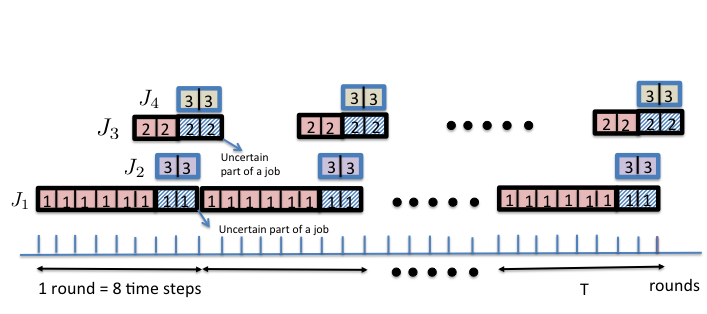
Refer to caption — Figure 1: Non-clairvoyant lower-bound instance

In our lower bound instance, we fix $n=2$ , and let $\ell_{i}(1)$ and $\ell_{i}(2)$ denote the losses of actions 1 and 2 in round $i$ as defined in Dekel et al. (2014). We map each round of the game to 8 time steps; that is, round $i$ corresponds to the time interval $[8i,8(i+1)-1]$ . Our instance has 4 sets of jobs $J_{1}$ , $J_{2}$ , $J_{3}$ , and $J_{4}$ , as shown in Figure 1. In each round, one job from each set arrives. Jobs in the set $J_{1}$ arrive at the beginning of each round; that is, at time steps $8i$ for $i=0,1,2,\ldots..T$ . The processing length of a job $j\in J_{1}$ that arrives in the round $i$ is 6 with probability $p_{i}(1)$ and 8 with probability $(1-p_{t}(1))$ , where $p_{i}(1)=1/2+\ell_{i}(1)/2$ . Observe that processing lengths of the jobs in $J_{1}$ depend on losses defined by Dekel et al. (2014). Further, the jobs in $J_{1}$ have a value of 1 per unit length. In round $i$ , a job from $J_{2}$ arrives at time $8(i+1)-2$ for $i=0,1,2,3,\ldots..T$ , and has a processing length of 2. The value per unit length of jobs in $J_{2}$ is 3.

The set $J_{3}$ consists of jobs that arrive at time instants $8i-3$ for $i=1,2,\ldots T$ , and have value per unit length of 2. The processing length of job $j\in J_{3}$ released in the round $i$ is 4 with probability $p_{i}(2)$ and 2 with probability $1-p_{i}(2)$ , where $p_{i}(2)=\ell_{i}(2)$ . Similar to the jobs in $J_{1}$ , the processing lengths of jobs in $J_{3}$ depend on the losses defined by the result of Dekel et al. (2014). Finally, the jobs in set $J_{4}$ are released at time steps $8i-1$ for $i=1,2,\ldots T$ , and have a processing length of 2 and value per unit length of 3.

The deadlines of all jobs are equal to their arrival times. (This condition is not necessary but simplifies the construction.) Hence, if a job is not scheduled upon its arrival, the algorithm loses the job.

Let $\texttt{ALG}_{1}$ and $\texttt{ALG}_{2}$ denote the two posted price scheduling mechanisms with prices 1 and 2 and FIFO scheduling policy. (Note that other posted price mechanisms, for example one that posts a price of 3, lose a constant factor in each round, hence we do not consider them.) The algorithms $\texttt{ALG}_{1}$ and $\texttt{ALG}_{2}$ correspond to the action set in the bandit problem with switching costs. The following two lemmas follow from the construction of lower bound instance. See Appendix C for a proof.

Lemma 5.2.

For all rounds $i=0,1,\ldots T$ , the expected value of $\texttt{ALG}_{1}$ in round $i$ is $10-2\ell_{i}(1)$ and expected value of $\texttt{ALG}_{2}$ in round $i$ is $10-2\ell_{i}(2)$ .

Lemma 5.3.

If an online algorithm switches from $\texttt{ALG}_{2}$ to $\texttt{ALG}_{1}$ in any round $i$ , it incurs a loss of at least 6.

From Lemmas 5.2 and 5.3, we get the following theorem.

Theorem 5.4.

Minimax regret of non-clairvoyant scheduling problem is at least $\tilde{\Omega}(T^{2/3})$ .

Consider an online scheduling algorithm for the non-clairvoyant scheduling problem. At the beginning of each round $i$ , it can either follow $\texttt{ALG}_{1}$ and obtain a value of $10-2\ell_{i}(1)$ or follow $\texttt{ALG}_{2}$ and get a value $10-2\ell_{i}(2)$ . Furthermore, since we are in the non-clairvoyant setting, the online algorithm won’t know the value it can obtain from the algorithm it is not following. Since, the value obtained by $\texttt{ALG}_{1}$ and $\texttt{ALG}_{2}$ are exactly the same in each round except for the terms $-\ell_{i}(1)$ and $-\ell_{i}(2)$ , the regret of the non-clairvoyant scheduling algorithm is equal to the regret it suffers on the losses at each round $i$ . Moreover, switching from $\texttt{ALG}_{2}$ to $\texttt{ALG}_{1}$ in any round incurs a cost of 6. Hence, our scheduling instance corresponds to bandit with switching cost problem, where switching from action 2 to action 1 incurs a cost. The result of Dekel et al. (2014) shows that the problem has a minimax regret of least $\tilde{\Omega}(T^{2/3})$ , when there is a switching cost between any pair of actions. However, it is easy to modify the proof in Dekel et al. (2014), where there is a switching cost only between action 2 to action 1, losing a factor of 2 in the regret bound Dekel et al. (2014). This completes our reduction.

Now we argue that Theorem (5.4) can be extended to random restarting benchmarks. Before that we make the following simple observation regarding the lower bound instance in Theorem (5.4). Consider the posted price mechanisms $\texttt{ALG}_{1}$ and $\texttt{ALG}_{2}$ as defined in the proof of Theorem (5.4). $\hbox to0.0pt{\hskip 7.61798pt\hbox{$\overline{\hbox{}}$}\hss}{\hbox{$\texttt{ALG}_{1}$}}(\gamma),{\hbox to0.0pt{\hskip 7.61798pt\hbox{$\overline{\hbox{}}$}\hss}{\hbox{$\texttt{ALG}_{2}$}}}(\gamma)$ denote the random restarting versions of them with restart parameter $\gamma$ .

Lemma 5.5.

For some constant $c\geq 11$ , we have:

j\in\{1,2\}:~~\text{\bf E}[W(\hbox to0.0pt{\hskip 10.4054pt\hbox{$\overline{\hbox{}}$}\hss}{\hbox{$\texttt{ALG}_{j}$}}(\gamma),J)]\geq W(\texttt{ALG}_{j},J)-c\cdot\gamma\cdot T

Proof of the lemma follows immediately from the observation that if $\texttt{ALG}_{j}$ for $j=1,2$ restarts at time $t$ , and $t$ is in round $i$ , then it loses values of jobs in that round. The expected number of restarts by the algorithms is at most $\gamma\cdot T$ . As the total value of jobs in each round is at most 11, the statement of the lemma holds for $c\geq 11$ .

To extend the lower bound to random restarting benchmarks, we need the following theorem from Dekel et al. (2014) for the bandit with switching costs problem.

Theorem 5.6 (Dekel et al. (2014)).

Let $\mathcal{A}$ be a multi-armed bandit algorithm that guarantees an expected regret (without switching costs) of $O(T^{\alpha})$ then there exists a sequence of loss functions that forces $\mathcal{A}$ to make $\tilde{\Omega}(T^{2(1-\alpha)})$ switches.

Combining Lemma 5.5 and above theorem, we prove the following theorem.

Theorem 5.7.

No online algorithm can achieve a regret $O(T^{2/3-\epsilon})$ for any $\epsilon>0$ against a random restarting benchmark with restart parameter $\gamma\in(T^{-1},T^{-1/3}]$ .

Proof is by contradiction. Suppose there is an online non-clairvoyant algorithm $\mathcal{A}$ that achieves a regret of $O(T^{2/3-\epsilon})$ for some $\epsilon>0$ . From Lemma 5.5, this implies that it achieves a regret of at most $O(T^{2/3-\epsilon})$ against the non-restarting benchmark of Theorem 5.4. Our proof of Theorem 5.4 gives a reduction from the bandit with switching cost problem to the non-clairvoyant scheduling problem. Therefore, we can invoke Theorem 5.6, which implies that $\mathcal{A}$ does at least $\tilde{\Omega}(T^{2(1-(2/3-\epsilon))})$ switches. Since there are only two actions in our lower bound instance, $\mathcal{A}$ still pays a switching cost of at least $\tilde{\Omega}(T^{2(1-(2/3-\epsilon))})=\tilde{\Omega}(T^{2/3+2\epsilon})$ in switching from $\texttt{ALG}_{2}$ to $\texttt{ALG}_{1}$ . This is gives a contradiction to the regret of $\mathcal{A}$ being $O(T^{2/3-\epsilon})$ against the non-restarting benchmark, and completes the proof.

References

Auer et al. (1995) Peter Auer, Nicolo Cesa-Bianchi, Yoav Freund, and Robert E Schapire. Gambling in a rigged casino: The adversarial multi-armed bandit problem. In Foundations of Computer Science, 1995. Proceedings., 36th Annual Symposium on, pages 322–331. IEEE, 1995.
Auer et al. (2007) Peter Auer, Ronald Ortner, and Csaba Szepesvári. Improved rates for the stochastic continuum-armed bandit problem. In International Conference on Computational Learning Theory, pages 454–468. Springer, 2007.
Azar and Khaitsin (2011) Yossi Azar and Ety Khaitsin. Prompt mechanism for ad placement over time. In International Symposium on Algorithmic Game Theory, pages 19–30. Springer, 2011.
Azar et al. (2015) Yossi Azar, Inna Kalp-Shaltiel, Brendan Lucier, Ishai Menache, Joseph Seffi Naor, and Jonathan Yaniv. Truthful online scheduling with commitments. In Proceedings of the Sixteenth ACM Conference on Economics and Computation, pages 715–732. ACM, 2015.
Blum and Burch (2000) Avrim Blum and Carl Burch. On-line learning and the metrical task system problem. Machine Learning, 39(1):35–58, 2000. ISSN 1573-0565. doi: 10.1023/A:1007621832648. URL http://dx.doi.org/10.1023/A:1007621832648.
Blum et al. (2002) Avrim Blum, Shuchi Chawla, and Adam Kalai. Static optimality and dynamic search-optimality in lists and trees. In Proceedings of the Thirteenth Annual ACM-SIAM Symposium on Discrete Algorithms, SODA ’02, pages 1–8, Philadelphia, PA, USA, 2002. Society for Industrial and Applied Mathematics. ISBN 0-89871-513-X. URL http://dl.acm.org/citation.cfm?id=545381.545382.
Canetti and Irani (1998) Ran Canetti and Sandy Irani. Bounding the power of preemption in randomized scheduling. SIAM Journal on Computing, 27(4):993–1015, 1998.
Cesa-Bianchi and Lugosi (2006) Nicolo Cesa-Bianchi and Gábor Lugosi. Prediction, learning, and games. Cambridge university press, 2006.
Chawla et al. (2017) Shuchi Chawla, Nikhil Devanur, Alexander Holroyd, Anna Karlin, James Martin, and Balasubramanian Sivan. Stability of service under time-of-use pricing. In STOC, 2017. To appear.
Cole et al. (2008) Richard Cole, Shahar Dobzinski, and Lisa Fleischer. Prompt mechanisms for online auctions. In International Symposium on Algorithmic Game Theory, pages 170–181. Springer, 2008.
Dekel et al. (2014) Ofer Dekel, Jian Ding, Tomer Koren, and Yuval Peres. Bandits with switching costs: T2/3 regret. In Proceedings of the Forty-sixth Annual ACM Symposium on Theory of Computing, STOC ’14, pages 459–467, New York, NY, USA, 2014. ACM. ISBN 978-1-4503-2710-7. doi: 10.1145/2591796.2591868. URL http://doi.acm.org/10.1145/2591796.2591868.
Eisenberg (2008) Bennett Eisenberg. On the expectation of the maximum of iid geometric random variables. Statistics & Probability Letters, 78(2):135–143, 2008.
Freund and Schapire (1995) Yoav Freund and Robert E Schapire. A desicion-theoretic generalization of on-line learning and an application to boosting. In European conference on computational learning theory, pages 23–37. Springer, 1995.
Hajiaghayi et al. (2005) Mohammad T. Hajiaghayi, Robert D. Kleinberg, Mohammad Mahdian, and David C. Parkes. Online auctions with re-usable goods. In Proceedings of the 6th ACM conference on Electronic commerce, pages 165–174. ACM, 2005.
Hartline and Roughgarden (2008) J. Hartline and T. Roughgarden. Optimal mechanism design and money burning. In Proc. 39th ACM Symp. on Theory of Computing, 2008.
Hutter et al. (2009) Frank Hutter, Holger H Hoos, Kevin Leyton-Brown, and Thomas Stützle. Paramils: an automatic algorithm configuration framework. Journal of Artificial Intelligence Research, 36(1):267–306, 2009.
Kalai and Vempala (2005) Adam Kalai and Santosh Vempala. Efficient algorithms for online decision problems. Journal of Computer and System Sciences, 71(3):291–307, 2005.
Lavi and Nisan (2015) Ron Lavi and Noam Nisan. Online ascending auctions for gradually expiring items. Journal of Economic Theory, 156:45–76, 2015.
Motwani and Raghavan (1995) Rajeev Motwani and Prabhakar Raghavan. Randomized Algorithms. Cambridge University Press, New York, NY, USA, 1995. ISBN 0-521-47465-5, 9780521474658.
Xu et al. (2008) Lin Xu, Frank Hutter, Holger H Hoos, and Kevin Leyton-Brown. Satzilla: portfolio-based algorithm selection for sat. Journal of artificial intelligence research, 32:565–606, 2008.

Appendix A Deferred proofs for upper bound constructions

Lemma 4.1.

If $A$ is an order respecting truthful mechanism, then $A$ with (arbitrary) restarts is also order respecting and truthful.

We assume that $A$ is restarted in the interval $[1,d_{\textrm{max}}+\ell_{\textrm{max}}]$ , and that the decision to restart is not dependent on what the jobs report. For a job that arrives by time 0, reporting an arrival time after 0 is not beneficial since that would mean that this job can only be processed beginning time $d_{\textrm{max}}+\ell_{\textrm{max}}+1$ , and the job would be past its deadline by then. If the job reports an arrival time before time 1, then truthfulness of $A$ guarantees that no misreport is beneficial.

Now consider a job $j$ that arrives after time 0. If the deadline of this job is such that it has to start by time $d_{\textrm{max}}+\ell_{\textrm{max}}$ , then no matter what it reports it does not get scheduled. For all other jobs, consider the instance where the jobs that arrive during the interval $[1,d_{\textrm{max}}+\ell_{\textrm{max}}]$ actually arrive at time $d_{\textrm{max}}+\ell_{\textrm{max}}+1$ , with the same arrival order. Truthfulness of $A$ for this instance guarantees truthfulness for such jobs.

Theorem 4.3.

Given order respecting truthful mechanisms $A$ and $B$ in the non-clairvoyant setting, switching mechanism $C$ in Definition 4.4 is order respecting, truthful, and obtains welfare at least

\textstyle\sum_{t\leq d_{\textrm{max}}+\ell_{\textrm{max}}}W_{t}(A)+\sum_{t\geq 1+d_{\textrm{max}}+\ell_{\textrm{max}}}W_{t}(B),

given that $A$ and $B$ are restarted at time 1.

The mechanism $C$ is order respecting by definition. Truthfulness of mechanism $C$ follows essentially from the truthfulness of restarts (Lemma 4.1). For any job that arrives before time 1, reporting an arrival time $\geq 1$ is not beneficial since it would only begin processing after $d_{\textrm{max}}+\ell_{\textrm{max}}$ by which time its deadline would have passed. If it reports a time before 1, then the truthfulness of $A$ guarantees that no misreport can be beneficial. For any job that arrives after time 0, the situation is exactly the same as a restart. What mechanism was run before time 1 has no bearing on the allocation and payments of this job. Lemma 4.1 guarantees truthfulness for these jobs.

The welfare guarantee follows from observing that mechanism $C$ completes all jobs that mechanism $A$ started before time 1, and that after time $d_{\textrm{max}}+\ell_{\textrm{max}}$ , the welfare of $C$ matches that of $B$ due to Lemma 4.2. The only loss of welfare is in the interval $[1,d_{\textrm{max}}+\ell_{\textrm{max}}]$ which is bounded by $v_{\textrm{max}}(d_{\textrm{max}}+\ell_{\textrm{max}})$ .

Appendix B Doubling Trick In the Multi-Armed Bandit Problem

In this section, we briefly explain the doubling trick. This helps with the case when algorithm $\texttt{Bandit-ALG}_{1}(R,T)$ (that admits a regret guarantee of $O(R\sqrt{T\log(T)})$ ) needs to know $R$ and $T$ in advance, and now we want to design an algorithm $\texttt{Bandit-ALG}_{2}$ that does not need knowing these parameters and still wants to achieve $O(R\sqrt{T\log(T)})$ regret bound (assuming $R$ and $T$ are finite). Doubling trick for time horizon $T$ is fairly standard, e.g. see Auer et al. (2007). We show how doubling trick works for range $R$ , and then how to merge the two doubling tricks.

Doubling trick for range $R$ .

For simplicity, suppose $R=2^{K}$ for some integer $K$ . $\texttt{Bandit-ALG}_{2}$ does the following. It starts with a guess (initialized to $1$ ) for $R$ and simulates $\texttt{Bandit-ALG}_{1}$ with this guess. Every time it sees a reward that is not in the guessed range, it doubles the guess (it may double it many times at the same time instance) and starts from scratch. Suppose $T_{1},T_{2},\ldots,T_{k}$ are the length of time intervals between two doubling. Therefore, for some constant $c>0$ ,

\textsc{Reg}(\texttt{Bandit-ALG}_{2})\leq\sum_{j=1}^{K}c.2^{j}\sqrt{T_{j}\log(T_{j})}\leq\sqrt{T\log(T)}\sum_{j=1}^{K}c.2^{j}=O(R\sqrt{T\log(T)})

Doubling trick for both range $R$ and time horizon $T$ .

In order to do so, use the doubling trick for $R$ as a black-box, and during the steps of doubling trick for $T$ , use this black-box.

Appendix C Deferred proofs for lower bound constructions

C.1 Lower bound of $\Omega(\sqrt{T})$ for the clairvoyant setting

Theorem 5.1.

There exists an instance of the clairvoyant scheduling problem where the regret of any online algorithm relative to the hindsight optimal posted-pricing-FIFO algorithm is $\Omega(\sqrt{T})$ .

Our proof is an adaptation of the lower bound instance for the problem of prediction with expert advice. Recall the lower bound of $\Omega(\sqrt{T})$ for the problem of prediction with expert advice. In this instance, we have two experts. In each round, the adversary chooses one of the two experts uniformly at random (and independently of the previous rounds), and assigns a reward of 1. The adversary sets the reward of the other expert to zero. The expected reward of any online algorithm is $T/2$ but suffers a regret of $\Omega(\sqrt{T})$ , as the expected reward of the best expert is $\text{\bf E}(\max\{\#\text{Heads},\#\text{Tails}\})=T/2+\Omega(\sqrt{T})$ . We adapt this lower bound to our scheduling problem as follows.

We map each round of the game to two time steps. We now describe our scheduling instance; we refer the reader to Figure 2. Let round $i$ of the game correspond to time steps $[t,t+1]$ . In our instance, all jobs have unit processing lengths. At time $t$ , we release two jobs: $j_{1}$ and $j_{2}$ . The deadline of job $j_{1}$ is $t+1$ whereas the deadline of job $j_{2}$ is $t+2$ . Job $j_{1}$ has a value of 1 and job $j_{2}$ has a value of 2. At time $t+1$ , we toss an unbiased coin. If the coin lands heads, we release job $j_{3}$ that has a deadline of $t+2$ and value 2. We repeat this instance in each round of the game.

Now consider two posted price algorithms $\texttt{ALG}_{1}$ and $\texttt{ALG}_{2}$ with prices 1 and $2$ and FIFO scheduling policy. It is easy to check that $\texttt{ALG}_{1}$ schedules jobs $j_{1}$ and $j_{2}$ in all rounds and obtains a total value of $3T$ . On the other hand, $\texttt{ALG}_{2}$ processes jobs $j_{2}$ in all the rounds, and processes jobs $j_{3}$ if it arrives, depending on the outcome of the coin toss. Therefore, the expected value obtained by $\texttt{ALG}_{2}$ is also $3T$ .

Consider the decision of an online algorithm at the beginning of each round. If it decides to schedule job $j_{1}$ , then the maximum value it can get in a round is equal to that of $\texttt{ALG}_{1}$ . On the other hand, if it decides schedule $j_{2}$ , then the maximum value it can get is equal to that of $\texttt{ALG}_{2}$ . Hence, the expected value obtained by any online algorithm is 3T.

Consider the expected value of the better of $\texttt{ALG}_{1}$ and $\texttt{ALG}_{2}$ . Let $\texttt{ALG}_{1}(i)$ and $\texttt{ALG}_{1}(i)$ denote the value obtained by the algorithms in round $i$ . Let $X_{i}$ denote a random variable that takes a value of 1 with probability 1/2 and -1 with probability 1/2.

$\displaystyle\text{\bf E}(\max\{\sum_{i}\texttt{ALG}_{1}(i),\sum_{i}\texttt{ALG}_{1}(2)\})$	$\displaystyle=$	$\displaystyle\text{\bf E}(\max\{3T,3T+\sum_{i}X_{i}\})$
	$\displaystyle=$	$\displaystyle 3T+\text{\bf E}(\max\{0,\sum_{i}X_{i}\})$
	$\displaystyle=$	$\displaystyle 3T+\Omega(\sqrt{T})$

Therefore, the regret of the online algorithm is at least $\Omega(\sqrt{T})$ .

C.2 Lower bound for the non-clairvoyant setting with random restarts

Lemma 5.2.

For all rounds $i=0,1,\ldots T$ , the expected value of $\texttt{ALG}_{1}$ in round $i$ is $10-2\ell_{i}(1)$ and expected value of $\texttt{ALG}_{2}$ in round $i$ is $10-2\ell_{i}(2)$ .

Consider $\texttt{ALG}_{1}$ . We note that $\texttt{ALG}_{1}$ only schedules jobs from the sets $J_{1}$ and $J_{2}$ . This is because, whenever $\texttt{ALG}_{1}$ finishes processing a job, there is a job belonging to $J_{1}$ or $J_{2}$ that is released exactly at that time and no jobs belonging to $J_{3}$ and $J_{4}$ are available for processing. Moreover, $\texttt{ALG}_{1}$ processes jobs from the set $J_{1}$ in all rounds, and it processes the job from $J_{3}$ if the processing length of job from $J_{1}$ is 6. This follows from our construction where the completion time of the job from $J_{1}$ with processing length 6 coincides exactly with the release time of the job from $J_{2}$ . Therefore, the expected reward obtained by $\texttt{ALG}_{1}$ in round $i$ is $6+2\cdot p_{i}(1)+(1-p_{i}(2))2\cdot 3=10-2\ell_{i}(1)$ .

Similarly, it is easy to check that $\texttt{ALG}_{2}$ only schedules jobs from the sets $J_{3}$ and $J_{4}$ . Therefore, the expected reward obtained by $\texttt{ALG}_{2}$ in round $i$ is $4+4\cdot p_{i}(2)+(1-p_{i}(2))2\cdot 3=10-2\ell_{i}(2)$ .

Lemma 5.3.

If an online algorithm switches from $\texttt{ALG}_{2}$ to $\texttt{ALG}_{1}$ in any round $i$ , it incurs a loss of at least 6.

We can assume that the switching times of the online algorithm correspond to the completion time of some job or idle periods. If the algorithm switches in the middle of processing a job, the lemma follows trivially since the value of every job in our instance is at least 6. Fix a round i, and consider a time instant $t$ when the algorithm switches from $\texttt{ALG}_{2}$ to $\texttt{ALG}_{1}$ . We consider two cases.

Case 1: Switching time $t$ corresponds to the completion time of a job from the set $J_{4}$ . In this case, $\texttt{ALG}_{1}$ is already processing a job from the set $J_{1}$ , and since deadlines of the jobs are same as arrival times, the online algorithm will not be able to schedule the job from the set $J_{1}$ . Therefore, the online algorithm loses a job of value of at least 6 in this round, which we charge to the switching cost.

Case 2: Switching time $t$ corresponds to the completion time of a job from the set $J_{3}$ . This case has two sub-cases depending on whether the job from the set $J_{3}$ had a processing length of 2 or 4. Suppose processing length of the job was 2. In this scenario, the online algorithm will not be able to process the job from the set $J_{4}$ , and hence loses a value of 6 in round $i$ . On the other hand, if the processing length of the job from the set $J_{3}$ was 4, then, the algorithm loses the job $j$ from set $J_{1}$ in the round $i+1$ , since the time of switch $t$ is greater than the deadline $d_{j}$ of the job.

In the both cases, the online algorithm loses a value of 6 in round $i$ , which we charge to the switching cost.

C.3 Linear lower bound for non-clairvoyant setting without random restarts, continuous time

Here we show that without our assumption regarding random restarting benchmark, no algorithm can get a sub-linear regret for the non-clairvoyant case, in a continuous time setting. By this we mean that the arrival time, deadline and processing lengths could be real numbers rather than integers.

Theorem C.1.

The minimax regret for the non-clairvoyant scheduling problem in a continuous time setting, compared against a benchmark without the random restart, is at least $\Omega(T)$ .

By Yao’s minimax principle Motwani and Raghavan (1995), we assume that our algorithm $\mathcal{A}$ is deterministic. We now give a distribution over jobs which proves the theorem.

We map each round of the game into two time steps. Similar to previous lower bound constructions, let $\texttt{ALG}_{1}$ and $\texttt{ALG}_{2}$ denote the two posted price scheduling mechanisms with prices 1 and 2 and FIFO scheduling policy. All jobs in our lower bound instance have tight deadlines. See Figure 3 for an illustration of the lower bound instance.

In the first round, the adversary releases two special jobs $j^{*}_{1}$ and $j^{*}_{2}$ . Job $j^{*}_{1}$ has a value 1 and job $j^{*}_{2}$ has a value 2; $j^{*}_{1}$ arrives slightly earlier than $j^{*}_{2}$ . From the definition, $\texttt{ALG}_{1}$ schedules $j^{*}_{1}$ and $\texttt{ALG}_{2}$ schedules $j^{*}_{2}$ . At the beginning of the game, the adversary tosses an unbiased coin. If the coin comes up heads, then adversary releases a set of jobs $S_{1}$ ; otherwise, a set of jobs $S_{2}$ is released.

The set $S_{1}$ consists of $T$ jobs, where $T$ is the number of rounds of the game. The value per unit length of each job is $2$ . The release time of a job $j\in S_{1}$ is $t+X_{j}$ , where $t$ is the beginning of round $i$ , and $X_{j}$ is a uniform $(0,1)$ random variable. The adversary chooses one of the $T$ jobs $j^{\prime}\in S_{1}$ uniformly at random, and makes it a long job by setting the processing length of the job $\ell_{j^{\prime}}=2$ . The remaining jobs in $S_{1}$ have length 1. Furthermore, the adversary correlates the processing length of the special job $j^{*}_{1}$ with the release time of the job $j^{\prime}$ , and sets it equal to $2+X_{j^{\prime}}$ . In other words, the completion time of the special job $j^{*}_{1}$ exactly coincides with the release time of $j^{\prime}$ . The adversary releases $S_{1}$ at the beginning of each round. Note that the random variables $X_{j}$ and the long job $j^{\prime}$ are sampled only in the beginning of game, and do not change over the course of the game.

From the construction it is easy to see that $\texttt{ALG}_{1}$ only schedules long jobs from the set $S_{1}$ , since the completion of the special job $j^{*}_{1}$ coincides with the release of the long job, and this repeats in each round till the game ends. The total value obtained by $\texttt{ALG}_{1}$ for this case is $2T$ since it schedules a long job in each round.

The set $S_{2}$ is constructed exactly same as the set $S_{1}$ , except for the following differences: 1) The value per unit length of each job is $2$ , and 2) the adversary correlates processing length of the special job $j^{*}_{2}$ with release time of the job $j^{\prime}\in S_{2}$ , and sets it equal to $2+Y_{j^{\prime}}$ , where $j^{\prime}$ denotes the long job in set $S_{2}$ . Also notice that random variables $Y_{j}$ for the set $S_{2}$ are different from the set $S_{1}$ , but are $(0,1)$ uniform random variables. Again from the construction it is easy to check that $\texttt{ALG}_{2}$ only schedules long jobs, since completion of the job $j^{*}_{2}$ coincides with the release of the long job, and this repeats in every round till the game ends. If the coin comes up tails, then the total value obtained by $\texttt{ALG}_{2}$ is $4T$ since it schedules a long job in each round.

Therefore, the expected value of the benchmark is at least $1/2\cdot 4T+1/2\cdot 4T=4T$ .

Now let us analyze the value obtained by an online algorithm $\mathcal{A}$ . For any realization of the job arrivals, only one of the two algorithms $\texttt{ALG}_{1}$ or $\texttt{ALG}_{2}$ generate non-trivial value. Since, this is chosen uniformly at random, we conclude that with probability half $\mathcal{A}$ follows the wrong algorithm in the first round. Therefore, if it needs to achieve a sub-linear regret it has to switch from the algorithm it followed in the first round to the other algorithm. Let us focus on the case when $\mathcal{A}$ switches from $\texttt{ALG}_{2}$ to $\texttt{ALG}_{1}$ at time $t$ .

Now, consider the situation faced by $\mathcal{A}$ at the beginning of the round $i$ that follows time $t$ . It sees $T$ jobs, each with value per unit length of 1, and arriving in the interval $[i,i+1]$ uniformly at random. One of these jobs is a long job, but $\mathcal{A}$ cannot distinguish this since we are in non-clairvoyant setting and the long job is chosen uniformly at random. Therefore, in expectation it takes $T/2$ rounds to identify the long job $\mathcal{A}$ . Hence, $\mathcal{A}$ schedules small jobs in $T/2$ rounds. This implies that in expectation $\mathcal{A}$ can only get a value of $T/2\cdot 1+T/2\cdot 4=2.5T$ . Similarly, it is easy to argue that if $\mathcal{A}$ switches from $\texttt{ALG}_{1}$ to $\texttt{ALG}_{2}$ it can get at most $T/2\cdot 1+T/2\cdot 4=2.5T$ . Therefore, the expected value obtained $\mathcal{A}$ on this distribution of jobs is at most $2.5T$ .

Therefore, it suffers a regret of $1.5T$ , and this completes our proof.

Truth and Regret in Online Scheduling

Abstract

1 Introduction

A Bayesian benchmark.

Challenges.

Our techniques.

Non-clairvoyance.

Outline.

2 Model and definitions

2.1 The online job scheduling problem

Online scheduling algorithms.

Regret minimization in online scheduling.

2.2 Learning from expert advice

Experts with switching costs.

Theorem 2.1 (Kalai and Vempala (2005)).

Multi-armed bandit setting.

Theorem 2.2 (Auer et al. (1995)).

3 The clairvoyant setting

3.1 Truthful switching

Lemma 3.1.

Theorem 3.2.

3.1.1 The online switching algorithm

Definition 3.1.

Design choices.

3.1.2 Truthfulness

Lemma 3.3.

Lemma 3.4.

3.1.3 Welfare

Lemma 3.5.

Lemma 3.6.

3.2 Reduction to experts with switching costs

Definition 3.2.

Theorem 3.7.

4 Non-clairvoyant setting

4.1 Scheduling algorithms with random restarts

Robustness of the benchmark.

Syncing issues.

Definition 4.1.

Definition 4.2.

Definition 4.3.

4.2 Truthful switching in the non-clairvoyant setting

Lemma 4.1.

Definition 4.4.

Lemma 4.2.

Theorem 4.3.

4.3 Reduction to multi-armed bandits

Definition 4.5.

Theorem 4.4.

Corollary 4.5.

Lemma 4.6 (Eisenberg (2008)).

5 Lower Bounds

Theorem 5.1.

Lemma 5.2.

Lemma 5.3.

Theorem 5.4.

Lemma 5.5.

Theorem 5.6 (Dekel et al. (2014)).

Theorem 5.7.

References

Appendix A Deferred proofs for upper bound constructions

Lemma 4.1.

Theorem 4.3.

Appendix B Doubling Trick In the Multi-Armed Bandit Problem

Doubling trick for range RR.

Doubling trick for both range RR and time horizon TT.

Appendix C Deferred proofs for lower bound constructions

C.1 Lower bound of Ω⁡(T)\Omega(\sqrt{T}) for the clairvoyant setting

Theorem 5.1.

C.2 Lower bound for the non-clairvoyant setting with random restarts

Lemma 5.2.

Lemma 5.3.

C.3 Linear lower bound for non-clairvoyant setting without random restarts, continuous time

Theorem C.1.

Doubling trick for range $R$ .

Doubling trick for both range $R$ and time horizon $T$ .

C.1 Lower bound of $\Omega(\sqrt{T})$ for the clairvoyant setting