跳到论文正文
W Papers独立论文阅读器 arXiv:1702.08662 论文正文 计算阅读时间 · 0%
引用这篇论文根据当前论文元数据生成,正式投稿前建议核对。


License: arXiv.org perpetual non-exclusive license
arXiv:1702.08662v4 [math.CO] 03 May 2017

The computational complexity of integer programming with alternationsThanks:  ⋆Department of Mathematics, UCLA, Los Angeles, CA, 90095.  Email:  {ldnguyen,pak}@math.ucla.eduThanks:  August 24, 2026

Danny Nguyen⋆ and Igor Pak⋆
Abstract.

We prove that integer programming with three alternating quantifiers is NP-complete, even for a fixed number of variables. This complements earlier results by Lenstra and Kannan, which together say that integer programming with at most two alternating quantifiers can be done in polynomial time for a fixed number of variables. As a byproduct of the proof, we show that for two polytopes P,Q⊂ℝ3P,Q\subset\mathbb{R}^{3}, counting the projection of integer points in Q\PQ\hskip 0.85355pt\backslash\hskip 0.85355ptP is #P-complete. This contrasts the 2003 result by Barvinok and Woods, which allows counting in polynomial time the projection of integer points in PP and QQ separately.

1. Introduction

1.1. Background

In a pioneer paper [Len83], Lenstra showed that Integer Programming in a bounded dimension can be solved in polynomial time. The next breakthrough was obtained by Kannan in 1990 and until recently remained the most general result in this direction (see [Eis10]).

Theorem 1.1 (Parametric Integer Programming [Kan90]).

Fix d1d_{1} and d2d_{2}. Given a polyhedron P⊆ℝd1P\subseteq\mathbb{R}^{d_{1}}, a matrix A∈ℤm×(d1+d2)A\in\mathbb{Z}^{m\times(d_{1}+d_{2})} and a vector b¯∈ℤm\overline{b}\in\mathbb{Z}^{m}, the following sentence can be decided in polynomial time:

(1.1) ∀𝐱∈P∩ℤd1∃𝐲∈ℤd2:A(𝐱,𝐲)≤b¯.\forall\hskip 0.85355pt\mathbf{x}\in P\cap\mathbb{Z}^{d_{1}}\quad\exists\hskip 0.85355pt\mathbf{y}\in\mathbb{Z}^{d_{2}}\quad:\quad A\,(\mathbf{x},\mathbf{y})\leq\overline{b}.

Here PP is given by a system C​𝐱≤γ¯C\,\mathbf{x}\leq\overline{\gamma}, with C∈ℤn×d1C\in\mathbb{Z}^{n\times d_{1}} and γ¯∈ℤn\overline{\gamma}\in\mathbb{Z}^{n}. The numbers m,nm,n are part of the input.

In [Kan92], Kannan asked if Theorem 1.1 can be extended to three alternating quantifiers. We give an answer in the negative direction to this question:

Theorem 1.2.

Fix d1≥1,d2≥2d_{1}\geq 1,d_{2}\geq 2 and d3≥3d_{3}\geq 3. Given two polyhedra P⊆ℝd1P\subseteq\mathbb{R}^{d_{1}}, Q⊆ℝd2Q\subseteq\mathbb{R}^{d_{2}}, a matrix A∈ℤm×(d1+d2+d3)A\in\mathbb{Z}^{m\times(d_{1}+d_{2}+d_{3})} and a vector b¯∈ℤm\overline{b}\in\mathbb{Z}^{m}, then deciding the sentence

(1.2) ∃𝐱∈P∩ℤd1∀𝐲∈Q∩ℤd2∃𝐳∈ℤd3:A(𝐱,𝐲,𝐳)≤b¯\exists\hskip 0.85355pt\mathbf{x}\in P\cap\mathbb{Z}^{d_{1}}\quad\forall\hskip 0.85355pt\mathbf{y}\in Q\cap\mathbb{Z}^{d_{2}}\quad\exists\hskip 0.85355pt\mathbf{z}\in\mathbb{Z}^{d_{3}}\quad:\quad A\,(\mathbf{x},\mathbf{y},\mathbf{z})\leq\overline{b}

is an NP-complete problem. Here PP and QQ are given by two systems C​𝐱≤γ¯C\,\mathbf{x}\leq\overline{\gamma} and D​𝐲≤δ¯D\,\mathbf{y}\leq\overline{\delta}, with C∈ℤn×d1C\in\mathbb{Z}^{n\times d_{1}}, γ¯∈ℤn\overline{\gamma}\in\mathbb{Z}^{n}, D∈ℤq×d2D\in\mathbb{Z}^{q\times d_{2}}, and δ¯∈ℤq\overline{\delta}\in\mathbb{Z}^{q}.

Let us emphasize that in both Theorem 1.1 and 1.2, there is no bound on the number of inequalities invovled. In other words, the parameters m,nm,n and qq are not fixed. Theorem 1.2 is especially surprising for the following reasons. First, in [NP17a], we gave strong evidence that (1.2) is decidable in polynomial time if m,nm,n and qq are fixed. Second, by an easy application of the Doignon–Bell–Scarf theorem, (1.1) is polynomial time reducible to the case with mm and nn fixed. Unfortunately, this simple reduction breaks down when there are more than two quantifiers (see Section 8.1) as in (1.2). Still, in [NP17a], we speculated that a more involved reduction argument might still apply to (1.2). Theorem 1.2 refutes the possibility of any reduction from (1.2) to an easier form with m,nm,n and qq bounded for which decision could be in polynomial time, unless P=NP\textup{{P}}={\textup{{NP}}}. In fact, Theorem 1.2 holds even when PP is an interval and QQ is an axis-parallel rectangles (see Theorem 4.1 and §\lx@sectionsign8.8). Thus, the problem (1.2) is already hard when n,qn,q are fixed and only mm is unbounded.

In [Sch97], Schöning proved that it is NP-complete to decide whether

(1.3) ∃x∈ℤ∀y∈ℤ:Ψ(x,y).\exists\hskip 0.85355ptx\in\mathbb{Z}\quad\forall\hskip 0.85355pty\in\mathbb{Z}\quad:\quad\Psi(x,y).

Compared to (1.2), this has only two quantifiers. However, here the expression Ψ⁡(x,y)\Psi(x,y) is allowed to contain both conjunctions and disjunctions of many inequalities. So Theorem 1.2 tells us that disjunctions can be discarded at the cost of adding one extra alternation. In the next subsection, we generalize this observation.

On can also consider a “hybrid” version of (1.2) and (1.3) with only 22 quantifiers ∃∀\exists\hskip 0.85355pt\forall\hskip 0.85355pt and only 22 disjunctions in Ψ\Psi. In Section 7, we show this is still NP-complete to decide.

1.2. Presburger sentences

In [Grä87], Grädel considered the theory of Presburger Arithmetic, and proved many completeness results in this theory when the number of variables and quantifiers are bounded. Those results were later strengthened by Schöning in [Sch97]. They can be summed up as follows:

Theorem 1.3 ([Sch97]).

Fix k≥1k\geq 1. Let Ψ⁡(𝐱,𝐲)\Psi(\mathbf{x},\mathbf{y}) be a Boolean combination of linear inequalities with integer coefficients in the variables 𝐱=(x1,…,xk)∈ℤk\mathbf{x}=(x_{1},\dots,x_{k})\in\mathbb{Z}^{k} and 𝐲=(y1,…,y3)∈ℤ3\mathbf{y}=(y_{1},\dots,y_{3})\in\mathbb{Z}^{3}. Then deciding the sentence

Q1x1∈ℤ…Qkxk∈ℤQk+1𝐲∈ℤ3:Ψ(𝐱,𝐲)Q_{1}\,x_{1}\in\mathbb{Z}\quad\dots\quad Q_{k}\,x_{k}\in\mathbb{Z}\quad Q_{k+1}\,\mathbf{y}\in\mathbb{Z}^{3}\quad:\quad\Psi(\mathbf{x},\mathbf{y})

is 𝚺kP\boldsymbol{\Sigma}^{\textup{{P}}}_{k}-complete if Q1=∃Q_{1}=\exists\hskip 0.85355pt, and 𝚷kP\boldsymbol{\Pi}^{\textup{{P}}}_{k}-complete if Q1=∀Q_{1}=\forall\hskip 0.85355pt. Here Q1,…,Qk+1∈{∀,∃}Q_{1},\dots,Q_{k+1}\in\{\forall\hskip 0.85355pt,\exists\hskip 0.85355pt\} are m+1m+1 alternating quantifiers.

This result characterizes the complexity of so called Presburger sentences with k+1k+1 quantifiers in a fixed number of variables. The main difference between Presburger Arithmetic versus integer programming is that the expression Ψ\Psi allows both conjunction and disjunction of many inequalities. This flexibility allows effective reductions of classical decision problems such as QSAT. For some time, it remains a question whether such reductions can be carried with only conjunctions, and at the same time keeping the number of variables fixed. We prove the following result, which generalizes Theorem 1.2:

Theorem 1.4.

Integer programming in a fixed number of variables with k+2k+2 alternating quantifiers is 𝚺kP/𝚷kP\boldsymbol{\Sigma}^{\textup{{P}}}_{k}/\boldsymbol{\Pi}^{\textup{{P}}}_{k}-complete, depending on whether Q1=∃/∀Q_{1}=\exists\hskip 0.85355pt/\forall\hskip 0.85355pt. Here the problem is allowed to contain only a system of inequalities.

We refer to Theorem 5.1 for the precise statement. Thus, we see that integer programming requires only one more quantifier alternation to achieve the same complexity as Presburger Arithmetic. Again, we emphasize that while the number of variables and quantifiers are fixed in Theorem 1.4, the linear system is still allowed many inequalities.

1.3. Counting points in projections of non-convex polyhedra

For polytopes in arbitrary dimension, counting the number of integer points points is classically #P-complete, even for 0/1 polytopes. In a fixed dimension dd, Barvinok famously showed this can be done in polynomial time:

Theorem 1.5 ([Bar93]).

Fix dd. Given a polytope P⊂ℝdP\subset\mathbb{R}^{d}, the number of integer points in P∩ℤdP\cap\mathbb{Z}^{d} can be computed in polynomial time. Here PP is described by a system A​𝐱≤b¯A\mathbf{x}\leq\overline{b}, with A∈ℤm×d,b¯∈ℤmA\in\mathbb{Z}^{m\times d},\,\overline{b}\in\mathbb{Z}^{m}.

For a set S⊂ℝdS\subset\mathbb{R}^{d}, denote by E​(S):=S∩ℤd{\text{\rm E}}(S):=S\cap\mathbb{Z}^{d}. The previous results say that |E​(P)||{\text{\rm E}}(P)| is computable in polynomial time. Given two polytopes P⊂Q⊂ℝdP\subset Q\subset\mathbb{R}^{d}, we clearly have |E​(Q\P)|=|E​(Q)|−|E​(P)||{\text{\rm E}}(Q\hskip 0.85355pt\backslash\hskip 0.85355ptP)|=|{\text{\rm E}}(Q)|-|{\text{\rm E}}(P)|. So the number of integer points in a complement can also be computed effectively.

Theorem 1.5 was later generalized by Barvinok and Woods to count the number of integer points in projections of polytopes:

Theorem 1.6 ([BW03]).

Fix d1d_{1} and d2d_{2}. Given a polytope P⊂ℝd1P\subset\mathbb{R}^{d_{1}}, and a linear transformation T:ℤd1→ℤd2T:\mathbb{Z}^{d_{1}}\to\mathbb{Z}^{d_{2}}, the number of integer points in T⁡(P∩ℤd1)T(P\cap\mathbb{Z}^{d_{1}}) can be computed in polynomial time. Here PP is described by a system A​𝐱≤b¯A\mathbf{x}\leq\overline{b} and TT is described by a matrix MM, where A∈ℤm×d1,b¯∈ℤmA\in\mathbb{Z}^{m\times d_{1}},\,\overline{b}\in\mathbb{Z}^{m} and M∈ℤd2×d1M\in\mathbb{Z}^{d_{2}\times d_{1}}.

For a set S⊂ℝdS\subset\mathbb{R}^{d}, denote by E1​(S){\text{\rm E}}_{1}(S) the projection of S∩ℤdS\cap\mathbb{Z}^{d} on the first coordinate, i.e.,

E1(S):={x∈ℤ:∃𝐳∈ℤd−1(x,𝐳)∈S}.{\text{\rm E}}_{1}(S)\,:=\,\{x\in\mathbb{Z}\quad:\quad\exists\hskip 0.85355pt\mathbf{z}\in\mathbb{Z}^{d-1}\quad(x,\mathbf{z})\in S\}.

By Theorem 1.6, |E1​(P)||{\text{\rm E}}_{1}(P)| can be computed in polynomial time for every polytope P⊂ℝdP\subset\mathbb{R}^{d}.

We prove the following result:

Theorem 1.7.

Given two polytopes P⊂Q⊂ℝ3P\subset Q\subset\mathbb{R}^{3}, computing |E1​(Q\P)||{\text{\rm E}}_{1}(Q\hskip 0.85355pt\backslash\hskip 0.85355ptP)| is #P-complete.

In other words, it is #P-complete to compute the size of the set

(1.4) E1(Q\P)={x∈ℤ:∃𝐳∈ℤ2(x,𝐳)∈Q\P}.{\text{\rm E}}_{1}(Q\hskip 0.85355pt\backslash\hskip 0.85355ptP)\hskip 1.70709pt=\hskip 1.70709pt\{x\in\mathbb{Z}\;:\;\exists\hskip 0.85355pt\mathbf{z}\in\mathbb{Z}^{2}\quad(x,\mathbf{z})\in Q\hskip 0.85355pt\backslash\hskip 0.85355ptP\}\hskip 0.85355pt.

Note that the corresponding decision problem |E1​(Q\P)|≥1|{\text{\rm E}}_{1}(Q\hskip 0.85355pt\backslash\hskip 0.85355ptP)|\geq 1 is equivalent to |E​(Q\P)|≥1|{\text{\rm E}}(Q\hskip 0.85355pt\backslash\hskip 0.85355ptP)|\geq 1, and thus can be decided in polynomial time by applying Theorem 1.5.

The contrast between Theorem 1.6 and our negative result can be explained as follows. The proof Theorem 1.6 depends on the polytopal structure of PP and exploited convexity in a crucial way. By taking the complement Q\PQ\hskip 0.85355pt\backslash\hskip 0.85355ptP, we no longer have a convex set. In other words, we show that projection of the complement Q\PQ\hskip 0.85355pt\backslash\hskip 0.85355ptP is complicated enough to allow encoding of hard counting problems, even in ℝ3\mathbb{R}^{3} (see also §\lx@sectionsign8.5).

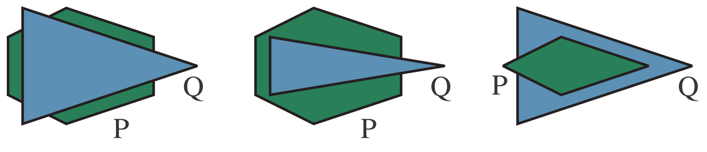
Refer to caption
Figure 1. Three examples of convex polygons P,Q⊂ℝ2P,Q\subset\mathbb{R}^{2}.
Remark 1.8.

To understand the theorem, consider three examples of polygons P,Q⊂ℝ2P,Q\subset\mathbb{R}^{2} as in Figure 1. Note that the sets of integer points of the vertical projections of P,QP,Q and P∪QP\cup Q are the same in all three cases, but the sets number of integer points of the vertical projections of Q\PQ\hskip 0.85355pt\backslash\hskip 0.85355ptP are quite different.

As an easy consequence of Theorem 1.7 we obtain:

Corollary 1.9.

Given rr simplices T1,…,Tr⊂ℝ3T_{1},\dots,T_{r}\subset\mathbb{R}^{3}, computing |E1​(T1∪⋯∪Tr)||{\text{\rm E}}_{1}(T_{1}\cup\dots\cup T_{r})| is #P-complete.

1.4. Outline of the paper

We begin with notations (Section 2) and a geometric construction of certain polytopes based on Fibonacci numbers (Section 3). In Section 4 we use this construction to prove Theorem 1.2 via a reduction of the GOOD SIMULTANEOUS APPROXIMATION (GSA) Problem in Number Theory, which is known to be NP-complete. The proof of Theorem 1.4 is via a reduction of QSAT (Section 5). The proof of Theorem 1.7 follows a similar route via reduction of #GSA (Section 6). Then we show that a “hybrid” version of (1.2) and (1.3) with only 22 quantifiers and 22 disjunctions is still NP-complete to decide (Section 7). Finally, we conclude with final remarks and open problems (Section 8).

2. Notations

We use ℕ={0,1,2,…}\mathbb{N}\hskip 0.85355pt=\hskip 0.85355pt\{0,1,2,\ldots\} and ℤ+={1,2,…}\mathbb{Z}_{+}=\{1,2,\ldots\}.

All constant vectors are denoted a¯,b¯,x¯,y¯,t¯\overline{a},\overline{b},\overline{x},\overline{y},\overline{t} etc.

Matrices are denoted A,B,CA,B,C, etc.

Variables are denoted x,y,zx,y,z, etc.; vectors of variables are denoted 𝐱,𝐲,𝐳\mathbf{x},\mathbf{y},\mathbf{z}, etc.

We write 𝐱≤𝐲\mathbf{x}\leq\mathbf{y} if xj≤yjx_{j}\leq y_{j} for all ii.

A polyhedron is an intersection of finitely many closed half-spaces in ℝn\mathbb{R}^{n}.

A polytope is a bounded polyhedron.

Polyhedra and polytopes are denoted by P,Q,RP,Q,R, etc.

3. Geometric constructions and properties

3.1. Fibonacci points

We consider the first 2​d2d Fibonacci numbers:

F0=0,F1=1,F2=1,…,F2​d−1.F_{0}=0,F_{1}=1,F_{2}=1,\dots,F_{2d-1}.

From these, we construct dd integer points:

(3.1) ϕ1=(F1,F0),ϕ2=(F3,F2),…,ϕd=(F2​d−1,F2​d−2).\phi_{1}=(F_{1},F_{0}),\;\phi_{2}=(F_{3},F_{2}),\;\dots,\;\phi_{d}=(F_{2d-1},F_{2d-2}).

Let

(3.2) Φ={ϕ1,…,ϕd}⊂ℤ2andJ=[1,F2​d−1]×[0,F2​d−2]∩ℤ2.\Phi=\{\phi_{1},\dots,\phi_{d}\}\subset\mathbb{Z}^{2}\quad\text{and}\quad J=[1,F_{2d-1}]\times[0,F_{2d-2}]\cap\mathbb{Z}^{2}.

We have Φ⊂J\Phi\subset J. Denote by 𝒞{\mathcal{C}} the curve consisting of d−1d-1 segments connecting ϕi\phi_{i} to ϕi+1\phi_{i+1} for i=1,…,i−1i=1,\dots,i-1.

We also define the following two polygons. Their properties will be mentioned later.

(3.3) R1={𝐲=(y1,y2)∈ℝ2:[y1≥1y2≤F2​d−2y2​F2​d−1−y1​F2​d−2≥1]},R_{1}=\Biggl\{\mathbf{y}=(y_{1},y_{2})\in\mathbb{R}^{2}\;:\;\left[\begin{smallmatrix}y_{1}&\geq&1\\ y_{2}&\leq&F_{2d-2}\\ y_{2}F_{2d-1}-y_{1}F_{2d-2}&\geq&1\end{smallmatrix}\right]\Biggr\},

and

(3.4) R2={𝐲∈ℝ2:[y1≤F2​d−1y2≥0] and y2F2​i−y1F2​i−1≤−2 for i=1,…,d}.R_{2}=\Biggl\{\mathbf{y}\in\mathbb{R}^{2}\;:\;\left[\begin{smallmatrix}y_{1}&\leq&F_{2d-1}\\ y_{2}&\geq&0\end{smallmatrix}\right]\text{ and }\;y_{2}F_{2i}-y_{1}F_{2i-1}\leq-2\;\text{ for }\;i=1,\dots,d\Biggr\}.

The following properties are straightforward from the above definitions:

  1. (F1)

    The points ϕ1,…,ϕd\phi_{1},\dots,\phi_{d} are in convex position. The curve 𝒞{\mathcal{C}} connecting them is convex (upwards). See Figure 2.

  2. (F2)

    Each segment (ϕi​ϕi+1)(\phi_{i}\hskip 1.70709pt\phi_{i+1}) and each triangle Δi=(0​ϕi​ϕi+1)\Delta_{i}=(0\hskip 1.70709pt\phi_{i}\hskip 1.70709pt\phi_{i+1}) has no interior integer points. This can be deduced from the facts that two consecutive Fibonacci numbers are coprime, and also

    Fi​Fi+3−Fi+1​Fi+2=(−1)i−1for all ​i≥0.F_{i}F_{i+3}-F_{i+1}F_{i+2}=(-1)^{i-1}\quad\text{for all }i\geq 0.
  3. (F3)

    The set of integer points in J\ΦJ\hskip 0.85355pt\backslash\hskip 0.85355pt\Phi can be partitioned into 22 parts: those lying strictly above the convex curve 𝒞{\mathcal{C}}, and those lying strictly below it.

  4. (F4)

    The part of J\ΦJ\hskip 0.85355pt\backslash\hskip 0.85355pt\Phi lying above 𝒞{\mathcal{C}} is exactly R1∩ℤ2R_{1}\cap\mathbb{Z}^{2}. This can be seen as follows. The line ℓ\ell connecting 00 and ϕd\phi_{d} is defined by:

    y2​F2​d−1−y1​F2​d−2=0.y_{2}F_{2d-1}-y_{1}F_{2d-2}=0.

    So every integer point 𝐲=(y1,y2)\mathbf{y}=(y_{1},y_{2}) lying above ℓ\ell satisfies:

    y2​F2​d−1−y1​F2​d−2≥1.y_{2}F_{2d-1}-y_{1}F_{2d-2}\geq 1.

    By property (F2), there are no integer points 𝐲\mathbf{y} between 𝒞{\mathcal{C}} and ℓ\ell. The other two edges of R1R_{1} come from JJ. See Figure 2.

  5. (F5)

    The part of J\ΦJ\hskip 0.85355pt\backslash\hskip 0.85355pt\Phi lying below 𝒞{\mathcal{C}} is exactly R2∩ℤ2R_{2}\cap\mathbb{Z}^{2}. This can be seen as follows. The line connecting ϕi\phi_{i} and ϕi+1\phi_{i+1} is defined by

    y2​F2​i−y1​F2​i−1=−1.y_{2}F_{2i}-y_{1}F_{2i-1}=-1.

    So all integer points below that line satisfies:

    y2​F2​i−y1​F2​i−1≤−2.y_{2}F_{2i}-y_{1}F_{2i-1}\leq-2.

    This gives d−1d-1 faces for R2R_{2}, one for each 1≤i≤d−11\leq i\leq d-1. The other two faces of R2R_{2} come from from JJ. See Figure 2.

R1R_{1}R2R_{2}00y2y_{2}y1y_{1}ϕd\phi_{d}ϕ1\phi_{1}⋰\iddots
Figure 2. The points ϕ1,…,ϕd∈Φ\phi_{1},\dots,\phi_{d}\in\Phi form a convex curve 𝒞{\mathcal{C}} (blue).

3.2. The polytopes

Given 𝜶=(α1,…,αd)∈ℚd\boldsymbol{\alpha}=(\alpha_{1},\dots,\alpha_{d})\in\mathbb{Q}^{d} and ϵ∈(0,12)∩ℚ\epsilon\in(0,\frac{1}{2})\cap\mathbb{Q}, for each 1≤i≤d1\leq i\leq d, we define a polygon:

(3.5) Pi={(x,w)∈ℝ2:1≤x≤N,αix−ϵ≤w≤αix+ϵ}.P_{i}=\big\{(x,w)\in\mathbb{R}^{2}\quad:\quad 1\leq x\leq N,\quad\alpha_{i}x-\epsilon\leq w\leq\alpha_{i}x+\epsilon\big\}.

Next, for each 1≤i≤d1\leq i\leq d, we define a new polygon

(3.6) Pi′={(x,ϕi,w):(x,w)∈Pi}⊂ℝ4.P^{\prime}_{i}=\big\{(x,\phi_{i},w)\;:\;(x,w)\in P_{i}\big\}\subset\mathbb{R}^{4}.

Finally, we define the convex hull:

(3.7) P=conv​(P1′,…,Pd′)⊂ℝ4.P={\text{\rm{conv}}}(P^{\prime}_{1},\dots,P^{\prime}_{d})\subset\mathbb{R}^{4}.

The following properties are straightforward from the above definitions:

  1. (P1)

    Each PiP_{i} is a parallelogram with vertices {(1,αi±ϵ),(N,αi​N±ϵ)}\big\{(1,\alpha_{i}\pm\epsilon),\,(N,\alpha_{i}N\pm\epsilon)\big\}.

  2. (P2)

    Each Pi′P^{\prime}_{i} is a parallelogram in ℝ4\mathbb{R}^{4} (i.e., a Minkowski sum of two intervals), with vertices {(1,ϕi,αi±ϵ),(N,ϕi,αi​N±ϵ)}\big\{(1,\phi_{i},\alpha_{i}\pm\epsilon),\,(N,\phi_{i},\alpha_{i}N\pm\epsilon)\big\}.

  3. (P3)

    The set of all vertices from P1′,…,Pd′P^{\prime}_{1},\dots,P^{\prime}_{d} are in convex position. Each Pi′P^{\prime}_{i} forms a 22-dimensional face of PP. This follows from from (3.6) and (F1).

  4. (P4)

    The polytope PP has 4​d4d vertices, which are all the vertices of P1′,…,Pd′P^{\prime}_{1},\dots,P^{\prime}_{d}.

  5. (P5)

    For every vertex (x,𝐲,w)(x,\mathbf{y},w) of PP, we have 𝐲=ϕi∈Φ\mathbf{y}=\phi_{i}\in\Phi for some 1≤i≤d1\leq i\leq d. Conversely, for every ϕi∈Φ\phi_{i}\in\Phi, we have:

    {(x,w)∈ℝ2:(x,ϕi,w)∈P}=Pi.\big\{(x,w)\in\mathbb{R}^{2}:(x,\phi_{i},w)\in P\big\}=P_{i}.

We will be using these properties in the latter sections.

4. Proof of Theorem 1.2

4.1.

By a box in ℤd\mathbb{Z}^{d}, we mean the set of integer points of the form [α1,β1]×⋯×[αd,βd]∩ℤd[\alpha_{1},\beta_{1}]\times\dots\times[\alpha_{d},\beta_{d}]\cap\mathbb{Z}^{d}. We will prove the following stronger version of Theorem 1.2.

Theorem 4.1.

Given a polytope U⊂ℝ6U\subset\mathbb{R}^{6} and two finite boxes I⊂ℤI\subset\mathbb{Z}, J⊂ℤ2J\subset\mathbb{Z}^{2}, deciding the sentence

(4.1) ∃x∈I∀𝐲∈J∃𝐳∈ℤ3:(x,𝐲,𝐳)∈U\exists\hskip 0.85355ptx\in I\quad\forall\hskip 0.85355pt\mathbf{y}\in J\quad\exists\hskip 0.85355pt\mathbf{z}\in\mathbb{Z}^{3}\quad:\quad(x,\mathbf{y},\mathbf{z})\in U

is an NP-complete problem. Here UU is described by a system A⁡(x,𝐲,𝐳)≤b¯A\,(x,\mathbf{y},\mathbf{z})\leq\overline{b}, where A∈ℤm×6A\in\mathbb{Z}^{m\times 6} and b¯∈ℤm\overline{b}\in\mathbb{Z}^{m}.

Since low dimensional boxes can be easily embedded into higher dimensions, the above implies Theorem 1.2 for every d1≥1,d2≥3d_{1}\geq 1,d_{2}\geq 3 and d3≥3d_{3}\geq 3. Compared to Theorem 1.2, all parameters in the above theorem are fixed, except for mm. So from now on, the symbols nn and dd will be reused for other purposes. For a vector 𝜶=(α1,…,αd)∈ℚd\boldsymbol{\alpha}=(\alpha_{1},\dots,\alpha_{d})\in\mathbb{Q}^{d} and an integer x∈ℤx\in\mathbb{Z}, we define

(4.2) {{x​𝜶}}=max1≤i≤d⁡{{q​αi}},\{\!\{x\boldsymbol{\alpha}\}\!\}=\max_{1\leq i\leq d}\{\!\{q\alpha_{i}\}\!\},

where for each rational β∈ℚ\beta\in\mathbb{Q}, the quantity {β}\{\beta\} is defined as:

{{β}}:=minn∈ℤ⁡|β−n|=min⁡{β−⌊β⌋,⌈β⌉−β}.\{\!\{\beta\}\!\}\hskip 1.70709pt:=\hskip 1.70709pt\min_{n\in\mathbb{Z}}|\beta-n|\hskip 1.70709pt=\hskip 1.70709pt\min\hskip 0.85355pt\bigl\{\beta-\lfloor\beta\rfloor,\lceil{\beta}\rceil-\beta\bigr\}\hskip 0.85355pt.
GOOD SIMULTANEOUS APPROXIMATION (GSA)
Input: A rational vector 𝜶=(α1,…,αd)∈ℚd\boldsymbol{\alpha}=(\alpha_{1},\dots,\alpha_{d})\in\mathbb{Q}^{d} and N∈ℕN\in{\mathbb{N}}, ϵ∈ℚ\epsilon\in\mathbb{Q}.
Decide: Is an integer x∈[1,N]x\in[1,N] such that {{x​𝜶}}≤ϵ\{\!\{x\boldsymbol{\alpha}\}\!\}\leq\epsilon\hskip 0.85355pt?

Note that GSA is only non-trivial for ϵ<1/2\epsilon<1/2. We need the following result by Lagarias:

Theorem 4.2 ([Lag85]).

GSA is NP-complete.

Let us emphasize that in GSA, the number dd is part of the input. If dd is fixed instead, then the problem can be decided in polynomial time (see [Lag85] and [GLS89, Ch. 5]). What follows is a reduction of GSA to a sentence of the form (4.1). GSA can be expressed as an integer programming problem:

(4.3) ∃x,w1,…,wd∈ℤ:1≤x≤N,−ϵ≤αix−wi≤ϵ.\exists\hskip 0.85355pt\,x,w_{1},\dots,w_{d}\in\mathbb{Z}\quad:\quad 1\leq x\leq N,\quad-\epsilon\leq\alpha_{i}x-w_{i}\leq\epsilon.

The inequalities on wiw_{i} can be expressed as (x,wi)∈Pi(x,w_{i})\in P_{i}, where PiP_{i} was defined in (3.5). Letting I=[1,N]∩ℤI=[1,N]\cap\mathbb{Z}, we see that GSA is equivalent to deciding:

(4.4) ∃x∈I:⋀i=1d[∃w∈ℤ:(x,w)∈Pi].\exists\hskip 0.85355ptx\in I\quad:\quad\bigwedge_{i=1}^{d}\Big[\exists\hskip 0.85355ptw\in\mathbb{Z}\;:\;(x,w)\in P_{i}\Big].
Lemma 4.3.

Let Φ={ϕ1,…,ϕd}\Phi=\{\phi_{1},\dots,\phi_{d}\} be as in (3.2) and PP be as in (3.7). We have:

(4.5) {{x𝜶}}≤ϵ⇔∀𝐲∈Φ∃w∈ℤ:(x,𝐲,w)∈P.\{\!\{x\boldsymbol{\alpha}\}\!\}\leq\epsilon\quad\iff\quad\forall\hskip 0.85355pt\mathbf{y}\in\Phi\quad\exists\hskip 0.85355ptw\in\mathbb{Z}:(x,\mathbf{y},w)\in P.
Proof.

Indeed, assume {{x​𝜶}}≤ϵ\{\!\{x\boldsymbol{\alpha}\}\!\}\leq\epsilon, i.e., xx satisfies GSA. By (4.4), for every i=1,…,di=1,\dots,d, there exists wi∈ℤw_{i}\in\mathbb{Z} with (x,wi)∈Pi(x,w_{i})\in P_{i}. Now (P5) implies that (x,ϕi,wi)∈P(x,\phi_{i},w_{i})\in P. Since this holds for every ϕi∈Φ\phi_{i}\in\Phi, the RHS in (4.5) is satisfied. For the other direction, assume the RHS in (4.5) holds. Then for every ϕi∈Φ\phi_{i}\in\Phi, there exists wi∈ℤw_{i}\in\mathbb{Z} with (x,ϕi,wi)∈P(x,\phi_{i},w_{i})\in P. By (P5), we have (x,wi)∈Pi(x,w_{i})\in P_{i}. By (4.4), xx satisfies GSA, i.e., {{x​𝜶}}≤ϵ\{\!\{x\boldsymbol{\alpha}\}\!\}\leq\epsilon. ∎

By the above lemma, GSA is equivalent to:

(4.6) ∃x∈I∀𝐲∈Φ∃w∈ℤ:(x,𝐲,w)∈P.\exists\hskip 0.85355ptx\in I\quad\forall\hskip 0.85355pt\mathbf{y}\in\Phi\quad\exists\hskip 0.85355ptw\in\mathbb{Z}:(x,\mathbf{y},w)\in P.

Consider JJ from (3.2), which contains Φ\Phi. We can rewrite the above sentence as:

(4.7) ∃x∈I∀𝐲∈J[(𝐲∈J\Φ)∨∃w∈ℤ:(x,𝐲,w)∈P].\exists\hskip 0.85355ptx\in I\quad\forall\hskip 0.85355pt\mathbf{y}\in J\quad\big[(\mathbf{y}\in J\hskip 0.85355pt\backslash\hskip 0.85355pt\Phi)\;\lor\;\exists\hskip 0.85355ptw\in\mathbb{Z}:(x,\mathbf{y},w)\in P\big].

Recall the polygons R1R_{1} and R2R_{2} defined in (3.3) and (3.4). By properties (F3), (F4) and (F5), we can rewrite 𝐲∈J\Φ\mathbf{y}\in J\hskip 0.85355pt\backslash\hskip 0.85355pt\Phi as (𝐲∈R1)∨(𝐲∈R2)(\mathbf{y}\in R_{1})\lor(\mathbf{y}\in R_{2}). Now, we can rewrite (4.7) as:

(4.8) ∃x∈I∀𝐲∈J[(𝐲∈R1)∨(𝐲∈R2)∨∃w∈ℤ:(x,𝐲,w)∈P].\exists\hskip 0.85355ptx\in I\quad\forall\hskip 0.85355pt\mathbf{y}\in J\quad\big[\,(\mathbf{y}\in R_{1})\;\lor\;(\mathbf{y}\in R_{2})\;\lor\;\exists\hskip 0.85355ptw\in\mathbb{Z}:(x,\mathbf{y},w)\in P\,\big].

Next, define two polytopes R1′R^{\prime}_{1} and R2′R^{\prime}_{2} as follows:

(4.9) Ri′:={(x,𝐲,0)∈ℝ4:0≤x≤N,𝐲∈Ri}⊂ℝ4fori=1,2.R^{\prime}_{i}\hskip 1.70709pt:=\hskip 0.85355pt\bigl\{(x,\mathbf{y},0)\in\mathbb{R}^{4}:0\leq x\leq N,\;\mathbf{y}\in R_{i}\bigr\}\hskip 0.85355pt\subset\mathbb{R}^{4}\quad\text{for}\quad i=1,2.

Polytopes R1′R^{\prime}_{1} and R2′R^{\prime}_{2} are defined in such a way so that for every x∈Ix\in I and 𝐲∈J\mathbf{y}\in J, we have 𝐲∈Ri\mathbf{y}\in R_{i} if and only if there exists w∈ℤw\in\mathbb{Z} such that (x,𝐲,w)∈Ri′(x,\mathbf{y},w)\in R^{\prime}_{i}.11 1 Such a ww must automatically be 00 by the definition of Ri′R^{\prime}_{i}. Now, it is clear that (4.8) is equivalent to:

∃x∈I∀𝐲∈J[(⋁i=12∃w∈ℤ:(x,𝐲,w)∈Ri′)∨(∃w∈ℤ:(x,𝐲,w)∈P)].\exists\hskip 0.85355ptx\in I\quad\forall\hskip 0.85355pt\mathbf{y}\in J\quad\Bigg[\Biggl(\,\bigvee_{i=1}^{2}\exists\hskip 0.85355ptw\in\mathbb{Z}:(x,\mathbf{y},w)\in R^{\prime}_{i}\,\Biggr)\;\lor\;\Biggl(\exists\hskip 0.85355ptw\in\mathbb{Z}:(x,\mathbf{y},w)\in P\Biggr)\,\Bigg].

which is equivalent to:

(4.10) ∃x∈I∀𝐲∈J∃w∈ℤ:(x,𝐲,w)∈R1′∪R2′∪P.\exists\hskip 0.85355ptx\in I\quad\forall\hskip 0.85355pt\mathbf{y}\in J\quad\exists\hskip 0.85355ptw\in\mathbb{Z}\quad:\quad(x,\mathbf{y},w)\in R^{\prime}_{1}\cup R^{\prime}_{2}\cup P.

The difference between (4.10) and (4.1) is that we have 33 polytopes instead of just one.

4.2.

The final step is two compress three polytopes R1′,R2′R^{\prime}_{1},R^{\prime}_{2} and PP into one polytope. Recall from (P4) that PP has 4​d4d vertices, which correspond to the vertices of all PiP_{i} for 1≤i≤d1\leq i\leq d. The vertices of R1R_{1} and R2R_{2} can be computed in polynomial time from systems (3.3) and (3.4). From there we easily get the vertices of R1′R^{\prime}_{1} and R2′R^{\prime}_{2}. Since P,R1′P,R^{\prime}_{1} and R2′R^{\prime}_{2} are in the fixed dimension 44, we can write down all their facets in polynomial time using their vertices. So we can represent:

(4.11) P\displaystyle P ={(x,𝐲,w)∈ℝ4:A1​(x,𝐲,w)≤b¯1},\displaystyle=\left\{(x,\mathbf{y},w)\in\mathbb{R}^{4}\;:\;A_{1}\,(x,\mathbf{y},w)\leq\overline{b}_{1}\right\},
R1′\displaystyle R^{\prime}_{1} ={(x,𝐲,w)∈ℝ4:A2​(x,𝐲,w)≤b¯2},\displaystyle=\left\{(x,\mathbf{y},w)\in\mathbb{R}^{4}\;:\;A_{2}\,(x,\mathbf{y},w)\leq\overline{b}_{2}\right\},
R2′\displaystyle R^{\prime}_{2} ={(x,𝐲,w)∈ℝ4:A3​(x,𝐲,w)≤b¯3}.\displaystyle=\left\{(x,\mathbf{y},w)\in\mathbb{R}^{4}\;:\;A_{3}\,(x,\mathbf{y},w)\leq\overline{b}_{3}\right\}.

The above three systems all have lengths polynomial in the input 𝜶,N\boldsymbol{\alpha},N and ϵ\epsilon. Next, we need the following lemma:

Lemma 4.4.

Fix nn and rr. Given rr polytopes R1,…,Rr⊂ℝnR_{1},\dots,R_{r}\subset\mathbb{R}^{n} described by rr systems

Ri={𝐱∈ℝn:Ai​𝐱≤b¯i},R_{i}=\{\mathbf{x}\in\mathbb{R}^{n}:A_{i}\,\mathbf{x}\leq\overline{b}_{i}\},

there is a polytope U∈ℝn+ℓU\in\mathbb{R}^{n+\ell}, where ℓ=⌈log2⁡r⌉\ell=\lceil\log_{2}r\rceil, such that

(4.12) 𝐱∈⋃i=1rRi∩ℤn⇔∃𝐭∈ℤℓ:(𝐱,𝐭)∈U∩ℤn+ℓ.\mathbf{x}\in\bigcup_{i=1}^{r}R_{i}\cap\mathbb{Z}^{n}\quad\iff\quad\exists\hskip 0.85355pt\mathbf{t}\in\mathbb{Z}^{\ell}:(\mathbf{x},\mathbf{t})\in U\cap\mathbb{Z}^{n+\ell}.

Furthermore, the system A⁡(𝐱,𝐭)≤b¯A\,(\mathbf{x},\mathbf{t})\leq\overline{b} that describes UU can be found in polynomial time, given AiA_{i}’s and b¯i\overline{b}_{i}’s as input.

Proof.

Let ℓ=⌈log2⁡r⌉\ell=\lceil\log_{2}r\rceil, we have 2ℓ≥r2^{\ell}\geq r. Pick t¯1,…,t¯r∈{0,1}ℓ\overline{t}_{1},\dots,\overline{t}_{r}\in\{0,1\}^{\ell} as rr different vertices of the ℓ\ell-dimensional unit cube. Define

Uj={(𝐱,t¯j)∈ℝn+ℓ:𝐱∈Rj}forj=1,…,r,U_{j}=\{(\mathbf{x},\overline{t}_{j})\in\mathbb{R}^{n+\ell}:\mathbf{x}\in R_{j}\}\quad\text{for}\quad j=1,\dots,r\,,

and

U=conv​(U1,…,Ur).U={\text{\rm{conv}}}(U_{1},\dots,U_{r}).

In other words, we form UjU_{j} by augmenting each RjR_{j} with ℓ\ell coordinates of t¯j\overline{t}_{j}. Since t¯1,…,t¯r\overline{t}_{1},\dots,\overline{t}_{r} are in convex position, so are the new polytopes U1,…,UjU_{1},\dots,U_{j}. So the vertices of UU are all the vertices of all UjU_{j}. Note that for every 𝐭∈conv​(t¯1,…,t¯r)\mathbf{t}\in{\text{\rm{conv}}}(\overline{t}_{1},\dots,\overline{t}_{r}), we have 𝐭∈ℤℓ\mathbf{t}\in\mathbb{Z}^{\ell} if and only if 𝐭=t¯j\mathbf{t}=\overline{t}_{j} for some jj. This implies that the only integer points in UU are those in UjU_{j}’s. In other words:

(𝐱,𝐭)∈U∩ℤn+ℓ⇔𝐱∈Rj∩ℤn and 𝐭=t¯j for some j=1,…,r.(\mathbf{x},\mathbf{t})\in U\cap\mathbb{Z}^{n+\ell}\quad\iff\quad\mathbf{x}\in R_{j}\cap\mathbb{Z}^{n}\;\text{ and }\;\mathbf{t}=\overline{t}_{j}\;\text{ for some }\;j=1,\dots,r.

So we have (4.12).

For each RjR_{j}, its vertices can be computed in polynomial time from the system Ai​𝐱≤b¯iA_{i}\,\mathbf{x}\leq\overline{b}_{i}. From these, we easily get the vertices for each UjU_{j}. Thus, we can find all vertices of UU in polynomial time. Note that UU is in a fixed dimesion n+ℓn+\ell, since nn and rr are fixed. Therefore, we can find in polynomial time all the facets of UU using those vertices. This gives us a system A⁡(𝐱,𝐭)≤b¯A\,(\mathbf{x},\mathbf{t})\leq\overline{b} of polynomial length that describes UU. ∎

Applying the above lemma for three polytopes R1′,R2′R^{\prime}_{1},R^{\prime}_{2} and PP with n=4n=4 and r=3r=3, we find a polytope U⊂ℝ4+ℓU\subset\mathbb{R}^{4+\ell} such that:

(4.13) (x,𝐲,w)∈(R1′∪R2′∪P)∩ℤ4⇔∃𝐭∈ℤℓ:(x,𝐲,w,𝐭)∈U∩ℤ4+ℓ.(x,\mathbf{y},w)\in(R^{\prime}_{1}\cup R^{\prime}_{2}\cup P)\cap\mathbb{Z}^{4}\quad\iff\quad\exists\hskip 0.85355pt\mathbf{t}\in\mathbb{Z}^{\ell}:(x,\mathbf{y},w,\mathbf{t})\in U\cap\mathbb{Z}^{4+\ell}.

Here we have ℓ=⌈log2⁡3⌉=2\ell=\lceil\log_{2}3\rceil=2, which means 𝐭∈ℤ2\mathbf{t}\in\mathbb{Z}^{2} and U⊂ℝ6U\subset\mathbb{R}^{6}. The lemma also allows us to find a system A⁡(x,𝐲,w,𝐭)≤b¯A\,(x,\mathbf{y},w,\mathbf{t})\leq\overline{b} that describes UU, which has size polynomial in the systems in (4.11). Now, we can rewrite (4.10) as:

∃x∈I∀𝐲∈J∃w∈ℤ:∃𝐭∈ℤ2(x,𝐲,w,𝐭)∈U,\exists\hskip 0.85355ptx\in I\quad\forall\hskip 0.85355pt\mathbf{y}\in J\quad\exists\hskip 0.85355ptw\in\mathbb{Z}\quad:\quad\exists\hskip 0.85355pt\mathbf{t}\in\mathbb{Z}^{2}\quad(x,\mathbf{y},w,\mathbf{t})\in U,

which is equivalent to

∃x∈I∀𝐲∈J∃𝐳∈ℤ3:A(x,𝐲,𝐳)≤b¯.\exists\hskip 0.85355ptx\in I\quad\forall\hskip 0.85355pt\mathbf{y}\in J\quad\exists\hskip 0.85355pt\mathbf{z}\in\mathbb{Z}^{3}\quad:\quad A\,(x,\mathbf{y},\mathbf{z})\leq\overline{b}.

Here 𝐳=(w,𝐭)∈ℤ3\mathbf{z}=(w,\mathbf{t})\in\mathbb{Z}^{3}. The final system A⁡(x,𝐲,𝐳)≤b¯A\,(x,\mathbf{y},\mathbf{z})\leq\overline{b} still has size polynomial in the original input 𝜶,N\boldsymbol{\alpha},N and ϵ\epsilon. Therefore, the original GSA problem is equivalent to (4.1). This implies that (4.1) is NP-hard.

It remains to show that (4.1) is in NP. We argue that more general sentence (1.2) is also in NP. From a result in [Grä87], if (1.2) is true, there must be an 𝐱\mathbf{x} satisfying it with length polynomial in the input P,AP,A and b¯\overline{b}. For such an 𝐱\mathbf{x}, we can apply Theorem 1.1 to check the rest of the sentence, which has the form ∀𝐲​∃𝐳\forall\hskip 0.85355pt\mathbf{y}\exists\hskip 0.85355pt\mathbf{z}, in polynomial time. This shows that deciding (1.2) is in NP, and thus NP-complete. □\square

5. Proof of Theorem 1.4

Recall the definition of boxes from Section 4. In this section, we prove:

Theorem 5.1.

Fix k≥1k\geq 1. Given a polytope U⊂ℝk+7U\subset\mathbb{R}^{k+7} and finite boxes I1,…,Ik⊂ℤI_{1},\dots,I_{k}\subset\mathbb{Z}, J⊂ℤ2J\subset\mathbb{Z}^{2}, K⊂ℤ5K\subset\mathbb{Z}^{5}, then the problem of deciding:

(5.1) Q1x1∈I1…Qkxk∈Ik∀𝐲∈J∃𝐳∈K:(𝐱,𝐲,𝐳)∈UQ_{1}\,x_{1}\in I_{1}\quad\dots\quad Q_{k}\,x_{k}\in I_{k}\,\quad\forall\hskip 0.85355pt\mathbf{y}\in J\quad\exists\hskip 0.85355pt\mathbf{z}\in K\quad:\quad(\mathbf{x},\mathbf{y},\mathbf{z})\in U

is 𝚺kP\boldsymbol{\Sigma}^{\textup{{P}}}_{k} complete if Q1=∃Q_{1}=\exists\hskip 0.85355pt, and 𝚷kP\boldsymbol{\Pi}^{\textup{{P}}}_{k} complete if Q1=∀Q_{1}=\forall\hskip 0.85355pt. Here Q1,…,Qk∈{∃,∀}Q_{1},\dots,Q_{k}\in\{\exists\hskip 0.85355pt,\forall\hskip 0.85355pt\} are kk alternating quantifiers with Qk=∃Q_{k}=\exists\hskip 0.85355pt. The polytope UU is described by a system A⁡(𝐱,𝐲,𝐳)≤b¯A\,(\mathbf{x},\mathbf{y},\mathbf{z})\leq\overline{b}, where A∈ℤm×(k+7)A\in\mathbb{Z}^{m\times(k+7)} and b¯∈ℤm\overline{b}\in\mathbb{Z}^{m}.

For the proof, we work with the canonical problem Q3SAT. Let Ψ\Psi a Boolean expression of the form:

(5.2) Ψ⁡(𝐮1,…,𝐮k)=⋀i=1N(ai∨bi∨ci).\Psi(\mathbf{u}_{1},\dots,\mathbf{u}_{k})=\bigwedge_{i=1}^{N}(a_{i}\lor b_{i}\lor c_{i}).

Here each 𝐮j=(uj​1,…,uj​ℓ)∈{0,1}ℓ\mathbf{u}_{j}=(u_{j1},\dots,u_{j\ell})\in\{0,1\}^{\ell} is a tuple of ℓ\hskip 0.85355pt\ell\hskip 0.85355pt Boolean variables, and each ai,bi,cia_{i},b_{i},c_{i} is a literal in the set {uj​s,¬uj​s: 1≤j≤k, 1≤s≤ℓ}\;\{u_{js},\;\lnot u_{js}\;:\;1\leq j\leq k,\;1\leq s\leq\ell\}. From Ψ\Psi, we construct a sentence:

(5.3) Q1𝐮1∈{0,1}ℓQ2𝐮2∈{0,1}ℓ…Qk𝐮k∈{0,1}ℓ:Ψ(𝐮1,…,𝐮k).Q_{1}\,\mathbf{u}_{1}\in\{0,1\}^{\ell}\quad Q_{2}\,\mathbf{u}_{2}\in\{0,1\}^{\ell}\;\dots\;Q_{k}\,\mathbf{u}_{k}\in\{0,1\}^{\ell}\quad:\quad\Psi(\mathbf{u}_{1},\dots,\mathbf{u}_{k}).

Here Q1,Q2,…,Qk∈{∀,∃}Q_{1},Q_{2},\dots,Q_{k}\in\{\forall\hskip 0.85355pt,\exists\hskip 0.85355pt\} are kk alternating quantifiers with Qk=∃Q_{k}=\exists\hskip 0.85355pt. The numbers ℓ\ell and NN are part of the input.

QUANTIFIED 3-SATISFIABILITY (Q3SAT)
Input: A Boolean expression Ψ\Psi of the form (5.2).
Decide: The truth of the sentence (5.3).

For clarity, we use the notation Q3SATk\textsc{Q3SAT}_{k} to emphasize problem (5.3) for a fixed kk. It is well-known that Q3SATk\textsc{Q3SAT}_{k} is 𝚺kP\boldsymbol{\Sigma}^{\textup{{P}}}_{k}-complete if Q1=∃Q_{1}=\exists\hskip 0.85355pt and 𝚷kP\boldsymbol{\Pi}^{\textup{{P}}}_{k}-complete if Q1=∀Q_{1}=\forall\hskip 0.85355pt (see e.g. [Pap94, MM11] and [AB09]). We proceed to reduce (5.3) to (5.1). In fact, by representing each Boolean string 𝐮j∈{0,1}ℓ\mathbf{u}_{j}\in\{0,1\}^{\ell} as an integer xj∈[0,2ℓ)x_{j}\in[0,2^{\ell}), we will only need to use I1=I2=⋯=Ik=[0,2ℓ)∩ℤI_{1}=I_{2}=\dots=I_{k}=[0,2^{\ell})\cap\mathbb{Z}.

For every string 𝐮j=(uj​1,…,uj​ℓ)∈{0,1}ℓ\,\mathbf{u}_{j}=(u_{j1},\dots,u_{j\ell})\in\{0,1\}^{\ell}\,, let xj∈[0,2ℓ)\,x_{j}\in[0,2^{\ell})\, be the corresponding integer in binary. Then uj​su_{js} is true or false respectively when the ss-th binary digit of xjx_{j} is 11 or 00. In other words, uj​su_{js} is true or false respectively when ⌊xj/2s−1⌋\lfloor x_{j}/2^{s-1}\rfloor is odd or even. Observe that t=⌊xj/2s−1⌋t=\lfloor x_{j}/2^{s-1}\rfloor is the only integer that satisfies xj/2s−1−1<t≤xj/2s−1x_{j}/2^{s-1}-1<t\leq x_{j}/2^{s-1}. Now, each term uj​su_{js} or ¬uj​s\lnot u_{js} can be expressed in xjx_{j} as follows:

(5.4) uj​s\displaystyle u_{js} ⇔∃w∈ℤ:{2​w+1>xj/2s−1−12​w+1≤xj/2s−1},\displaystyle\iff\exists\hskip 0.85355ptw\in\mathbb{Z}\;:\;\begin{Bmatrix}2w+1&>&x_{j}/2^{s-1}-1\\ 2w+1&\leq&x_{j}/2^{s-1}\end{Bmatrix},
¬uj​s\displaystyle\lnot u_{js} ⇔∃w∈ℤ:{2​w>xj/2s−1−12​w≤xj/2s−1}.\displaystyle\iff\exists\hskip 0.85355ptw\in\mathbb{Z}\;:\;\begin{Bmatrix}2w&>&x_{j}/2^{s-1}-1\\ 2w&\leq&x_{j}/2^{s-1}\end{Bmatrix}.

Let 𝐱=(x1,…,xk)∈[0,2ℓ)k\mathbf{x}=(x_{1},\dots,x_{k})\in[0,2^{\ell})^{k}. Recall that each term ai,bi,cia_{i},b_{i},c_{i} in (5.2) is uj​su_{js} or ¬uj​s\lnot u_{js} for some jj and ss. So each clause ai∨bi∨cia_{i}\lor b_{i}\lor c_{i} can be expressed in 𝐱\mathbf{x} as:

(5.5) ai∨bi∨ci⇔∃w∈ℤ:[Di(𝐱,w)≤d¯i]∨[Ei(𝐱,w)≤e¯i]∨[Fi(𝐱,w)≤f¯i],a_{i}\lor b_{i}\lor c_{i}\iff\exists\hskip 0.85355ptw\in\mathbb{Z}\;:\;\big[D_{i}\,(\mathbf{x},w)\leq\overline{d}_{i}\big]\lor\big[E_{i}(\mathbf{x},w)\leq\overline{e}_{i}\big]\lor\big[F_{i}\,(\mathbf{x},w)\leq\overline{f}_{i}\big],

where three systems Di​(𝐱,w)≤d¯i,Ei​(𝐱,w)≤e¯i,Fi​(𝐱,w)≤f¯i\,D_{i}\,(\mathbf{x},w)\leq\overline{d}_{i},\;E_{i}(\mathbf{x},w)\leq\overline{e}_{i},\;F_{i}\,(\mathbf{x},w)\leq\overline{f}_{i}\, are of the form (5.4) (with different jj and ss for each). Note that the strict inequalities in (5.4) can be sharpened without losing any integer solutions (see Remark 6.2). We define the polytopes:

Ki\displaystyle K_{i} ={(𝐱,w)∈ℝk+1:x1,…,xk,w∈[0,2ℓ),Di(𝐱,w)≤d¯i},\displaystyle=\big\{(\mathbf{x},w)\in\mathbb{R}^{k+1}\;:\;x_{1},\dots,x_{k},w\in[0,2^{\ell}),\;D_{i}\,(\mathbf{x},w)\leq\overline{d}_{i}\big\},
Li\displaystyle L_{i} ={(𝐱,w)∈ℝk+1:x1,…,xk,w∈[0,2ℓ),Ei(𝐱,w)≤e¯i},\displaystyle=\big\{(\mathbf{x},w)\in\mathbb{R}^{k+1}\;:\;x_{1},\dots,x_{k},w\in[0,2^{\ell}),\;E_{i}\,(\mathbf{x},w)\leq\overline{e}_{i}\big\},
Mi\displaystyle M_{i} ={(𝐱,w)∈ℝk+1:x1,…,xk,w∈[0,2ℓ),Fi(𝐱,w)≤f¯i}.\displaystyle=\big\{(\mathbf{x},w)\in\mathbb{R}^{k+1}\;:\;x_{1},\dots,x_{k},w\in[0,2^{\ell}),\;F_{i}\,(\mathbf{x},w)\leq\overline{f}_{i}\big\}.

So the RHS in (5.5) can be rewritten as:

∃w∈ℤ:(𝐱,w)∈Ki∪Li∪Mi.\exists\hskip 0.85355ptw\in\mathbb{Z}\;:\;(\mathbf{x},w)\in K_{i}\cup L_{i}\cup M_{i}.

Let I1=I2=⋯=Ik=[0,2ℓ)∩ℤI_{1}=I_{2}=\dots=I_{k}=[0,2^{\ell})\cap\mathbb{Z}, we see that (5.3) is equivalent to:

(5.6) Q1x1∈I1…Qkxk∈Ik:⋀i=1N[∃w∈ℤ:(𝐱,w)∈Ki∪Li∪Mi].Q_{1}\,x_{1}\in I_{1}\quad\dots\quad Q_{k}\,x_{k}\in I_{k}\quad:\quad\bigwedge_{i=1}^{N}\Big[\exists\hskip 0.85355ptw\in\mathbb{Z}\;:\;(\mathbf{x},w)\in K_{i}\cup L_{i}\cup M_{i}\Big].

For each ii, we apply Lemma 4.4 (with n=k+1,r=3n=k+1,\,r=3) to the polytopes Ki,Li,Mi⊂ℝk+1K_{i},L_{i},M_{i}\subset\mathbb{R}^{k+1}. This gives us another polytope Gi⊂ℝk+3G_{i}\subset\mathbb{R}^{k+3} that satisfies:

(𝐱,w)∈Ki∪Li∪Mi⇔∃𝐯∈ℤ2:(𝐱,w,𝐯)∈Gi.(\mathbf{x},w)\in K_{i}\cup L_{i}\cup M_{i}\quad\iff\quad\exists\hskip 0.85355pt\mathbf{v}\in\mathbb{Z}^{2}\;:\;(\mathbf{x},w,\mathbf{v})\in G_{i}.

Substituting this into (5.6), we have an equivalent sentence:

(5.7) Q1x1∈I1…Qkxk∈Ik:⋀i=1N[∃𝐰∈ℤ3:(𝐱,𝐰)∈Gi],Q_{1}\,x_{1}\in I_{1}\quad\dots\quad Q_{k}\,x_{k}\in I_{k}\,\quad:\quad\bigwedge_{i=1}^{N}\Big[\exists\hskip 0.85355pt\mathbf{w}\in\mathbb{Z}^{3}\;:\;(\mathbf{x},\mathbf{w})\in G_{i}\Big],

where 𝐰=(w,𝐯)∈ℤ3\mathbf{w}=(w,\mathbf{v})\in\mathbb{Z}^{3}, and each Gi⊂ℝk+3G_{i}\subset\mathbb{R}^{k+3}.

Notice that apart from the outer quantifiers, (5.7) is a direct analogue of (4.4), with GiG_{i} playing the role of PiP_{i} and (𝐱,𝐰)(\mathbf{x},\mathbf{w}) in place of (x,w)(x,w). The proof now proceeds similarly to the rest of Section 4 after (4.4). Along the proof, we need to define Gi′G^{\prime}_{i} and GG in similar manners to (3.6) and (3.7). The variable 𝐲∈ℤ2\mathbf{y}\in\mathbb{Z}^{2} is again needed to define Gi′G^{\prime}_{i}. Φ\Phi and JJ from (3.2) are reused without change. This gives us Gi′,G⊂ℝk+5G^{\prime}_{i},G\subset\mathbb{R}^{k+5}. At the end of the proof, we also need to apply Lemma 4.4 one more time to produce a single polytope UU, just like in (4.13). The dimension 44 in (4.13) is now k+5k+5. As a result, the final polytope UU has dimension k+7k+7. In the final form (5.1), we will have 𝐱∈ℤk,𝐲∈ℤ2\mathbf{x}\in\mathbb{Z}^{k},\mathbf{y}\in\mathbb{Z}^{2} and 𝐳=(𝐰,𝐭)∈ℤ5\mathbf{z}=(\mathbf{w},\mathbf{t})\in\mathbb{Z}^{5}.

We have converted (5.3) to an equivalent sentence (5.1) with polynomial size. This shows that (5.1) is 𝚺kP\boldsymbol{\Sigma}^{\textup{{P}}}_{k}/𝚷kP\boldsymbol{\Pi}^{\textup{{P}}}_{k}-hard depending when Q1=∃/∀Q_{1}=\exists\hskip 0.85355pt/\forall\hskip 0.85355pt. For each tuple 𝐱=(x1,…,xk)\mathbf{x}=(x_{1},\dots,x_{k}), we can check in polynomial time whether ∀𝐲∈J​∃𝐳∈K:A⁡(𝐱,𝐲,𝐳)≤b¯\forall\hskip 0.85355pt\mathbf{y}\in J\;\;\exists\hskip 0.85355pt\mathbf{z}\in K\;:\;A\,(\mathbf{x},\mathbf{y},\mathbf{z})\leq\overline{b}\; by applying Theorem 1.1. This shows the membership of (5.1) in 𝚺kP\boldsymbol{\Sigma}^{\textup{{P}}}_{k}/𝚷kP\boldsymbol{\Pi}^{\textup{{P}}}_{k}. We conclude that (5.1) is 𝚺kP\boldsymbol{\Sigma}^{\textup{{P}}}_{k}/𝚷kP\boldsymbol{\Pi}^{\textup{{P}}}_{k}-complete when Q1=∃/∀Q_{1}=\exists\hskip 0.85355pt/\forall\hskip 0.85355pt. □\square

6. Proof of Theorem 1.7

6.1.

Now we prove Theorem 1.7. We use the same construction as in the proof of Theorem 1.2. Recall the definition of {{x​𝜶}}\{\!\{x\boldsymbol{\alpha}\}\!\} from Section 4. We reduce the following counting problem to a problem of the form (1.4):

#GOOD SIMULTANEOUS APPROXIMATIONS (#GSA)
Input: A rational vector 𝜶=(α1,…,αd)∈ℚd\boldsymbol{\alpha}=(\alpha_{1},\dots,\alpha_{d})\in\mathbb{Q}^{d} and N∈ℕN\in{\mathbb{N}}, ϵ∈ℚ\epsilon\in\mathbb{Q}.
Output: The number of integers x∈[1,N]x\in[1,N] that satisfy {{x​𝜶}}≤ϵ\{\!\{x\boldsymbol{\alpha}\}\!\}\leq\epsilon\hskip 0.85355pt.

The argument in [Lag85] is based on a parsimonious reduction. Namely, it gives a bijection between solutions for #​GSA\#\textsc{GSA} and the following problem:

#WEAK PARTITIONS
Input: An integer vector a¯=(a1,…,ad)∈ℤd\overline{a}=(a_{1},\dots,a_{d})\in\mathbb{Z}^{d}.
Output: The number of 𝐲∈{−1,0,1}d\mathbf{y}\in\{-1,0,1\}^{d} for which a¯⋅𝐲=0\overline{a}\cdot\mathbf{y}=0.

It is well known and easy to see that #WEAK PARTITIONS is #P-complete. The decision version WEAK PARTITION was earlier shown by [vEB81] to be NP-complete with a parsimonious reduction from KNAPSACK. Together with Lagarias’s reduction, we conclude:

Theorem 6.1.

#GSA is #P-complete.

6.2.

Now we proceed with the reduction of #GSA to (1.4).

Just like the decision version, #GSA is only non-trivial for ϵ<1/2\epsilon<1/2. Define:

(6.1) Qi={(x,w)∈ℝ2:1≤x≤N,αix+ϵ<w<αix−ϵ+1}.Q_{i}=\big\{(x,w)\in\mathbb{R}^{2}\quad:\quad 1\leq x\leq N,\quad\alpha_{i}x+\epsilon<w<\alpha_{i}x-\epsilon+1\big\}.

Let I=[1,N]∩ℤI=[1,N]\cap\mathbb{Z}. We have:

Observation 1.

An x∈Ix\in I satisfies {{x​𝜶}}≤ϵ\{\!\{x\boldsymbol{\alpha}\}\!\}\leq\epsilon\hskip 0.85355pt if and only if for every 1≤i≤d1\leq i\leq d, there is no w∈ℤw\in\mathbb{Z} such that (x,w)∈Qi(x,w)\in Q_{i}.

Indeed, consider x∈Ix\in I. By (4.3), we have {{x​𝜶}}≤ϵ\{\!\{x\boldsymbol{\alpha}\}\!\}\leq\epsilon if and only if for each ii, there exists wi∈ℤw_{i}\in\mathbb{Z} with wi∈[αi​x−ϵ,αi​x+ϵ]w_{i}\in[\alpha_{i}x-\epsilon,\alpha_{i}x+\epsilon]. This interval of length 2​ϵ2\epsilon is contained in [αix−ϵ,αix−ϵ+1)[\alpha_{i}x-\epsilon,\alpha_{i}x-\epsilon+1). The latter is a half-open unit interval, which always contains a unique integer wiw_{i}. So wi∈[αi​x−ϵ,αi​x+ϵ]w_{i}\in[\alpha_{i}x-\epsilon,\alpha_{i}x+\epsilon] if and only if wi∉(αi​x+ϵ,αi​x−ϵ+1)w_{i}\notin(\alpha_{i}x+\epsilon,\alpha_{i}x-\epsilon+1). In other words, for each 1≤i≤d1\leq i\leq d, there should be no w∈ℤw\in\mathbb{Z} with (x,w)∈Qi(x,w)\in Q_{i}. The converse is also straightforward.

Remark 6.2.

Note that each QiQ_{i} has two open edges. They can actually sharpened without affecting the integer points in QiQ_{i}. Indeed, we can multiply each inequality with the denominators in αi\alpha_{i} and ϵ\epsilon, which have polynomial length. Each resulting inequality is of the form a<ba<b, with aa and bb having integer values. This is equivalent to a≤b−1a\leq b-1. Therefore, we can replace QiQ_{i} with a (smaller) closed parallelogram containing the same integer points.

By the above observation, #GSA asks for:

(6.2) N−#{x∈I:∃1≤i≤d∃w∈ℤ(x,w)∈Qi}.N\;-\;\#\Big\{x\in I\;:\;\exists\hskip 0.85355pt1\leq i\leq d\quad\exists\hskip 0.85355ptw\in\mathbb{Z}\quad(x,w)\in Q_{i}\Big\}.

We convert the union of QiQ_{i} into a complement V\UV\hskip 0.85355pt\backslash\hskip 0.85355ptU of two polytopes U,V⊂ℝ3U,V\subset\mathbb{R}^{3}.

6.3.

Let T=1+N​maxi​αiT=1+N\max_{i}\alpha_{i}. Pick dd integers 0<m1<m2<⋯<md0<m_{1}<m_{2}<\dots<m_{d} so that

(6.3) mi−1+mi+12+2​T<mifor2≤i≤d−1.\frac{m_{i-1}+m_{i+1}}{2}+2T<m_{i}\quad\text{for}\quad 2\leq i\leq d-1.

We embed each parallelogram QiQ_{i} into ℝ3\mathbb{R}^{3} as

(6.4) Ri={(x,y,w)∈ℝ3:(x,w−mi)∈Qi,y=i}.R_{i}=\big\{(x,y,w)\in\mathbb{R}^{3}\;:\;(x,w-m_{i})\in Q_{i},\;y=i\big\}.

In other words, we translate QiQ_{i} by mim_{i} in the direction ww, and embed it into the plane y=iy=i inside ℝ3\mathbb{R}^{3} (see Figure 3). The following is obvious:

Observation 2.

For each x∈Ix\in I and 1≤i≤d1\leq i\leq d, there exists w∈ℤw\in\mathbb{Z} with (x,w)∈Qi(x,w)\in Q_{i} if and only if there exists (y,w)∈ℤ2(y,w)\in\mathbb{Z}^{2} with (x,y,w)∈Ri(x,y,w)\in R_{i}.

Denote by Ai,Bi,CiA_{i},B_{i},C_{i} and DiD_{i} the vertices of RiR_{i}. Let Ki=(N,i,0)K_{i}=(N,i,0) and Li=(1,i,0)L_{i}=(1,i,0) for each 1≤i≤d1\leq i\leq d. Define:

(6.5) U\displaystyle U =conv{Ai,Bi,Ki,Li: 1≤i≤d}⊂ℝ3,\displaystyle={\text{\rm{conv}}}\big\{A_{i},\hskip 0.85355ptB_{i},\hskip 0.85355ptK_{i},\hskip 0.85355ptL_{i}\,:\,1\leq i\leq d\big\}\subset\mathbb{R}^{3},
V\displaystyle V =conv{Ci,Di,Ki,Li: 1≤i≤d}⊂ℝ3.\displaystyle={\text{\rm{conv}}}\big\{C_{i},\hskip 0.85355ptD_{i},\hskip 0.85355ptK_{i},\hskip 0.85355ptL_{i}\,:\,1\leq i\leq d\big\}\subset\mathbb{R}^{3}.
Refer to caption
Figure 3. The parallelograms RiR_{i}.

Since conv​(Ai,Bi,Ki,Li)⊂conv​(Ci,Di,Ki,Li){\text{\rm{conv}}}(A_{i},B_{i},K_{i},L_{i})\subset{\text{\rm{conv}}}(C_{i},D_{i},K_{i},L_{i}) for each 1≤i≤d1\leq i\leq d, we have U⊂VU\subset V. It is also clear that:

(6.6) Ri=conv​(Ci,Di,Ki,Li)\conv​(Ai,Bi,Ki,Li).R_{i}={\text{\rm{conv}}}(C_{i},D_{i},K_{i},L_{i})\hskip 0.85355pt\backslash\hskip 0.85355pt{\text{\rm{conv}}}(A_{i},B_{i},K_{i},L_{i}).

Denote by {y=i}\{y=i\} the plane y=iy=i.

Observation 3.

We have U∩{y=i}=conv(Ai,Bi,Ki,Li)U\cap\{y=i\}={\text{\rm{conv}}}(A_{i},B_{i},K_{i},L_{i}). Similarly, V∩{y=i}=conv(Ci,Di,Ki,Li)V\cap\{y=i\}={\text{\rm{conv}}}(C_{i},D_{i},K_{i},L_{i}).

Indeed, from (6.5), it is clear that conv​(Ai,Bi,Ki,Li){\text{\rm{conv}}}(A_{i},B_{i},K_{i},L_{i}) lies in both UU and the plane y=iy=i. On the other hand, if (x,i,w)∈U(x,i,w)\in U, it must be a convex combination of Aj,Bj,Kj,LjA_{j},B_{j},K_{j},L_{j} for 1≤j≤d1\leq j\leq d. First, assume that

(6.7) (x,i,w)∈conv{Aj,Bj,Kj,Lj:j≠i}.(x,i,w)\in{\text{\rm{conv}}}\big\{A_{j},B_{j},K_{j},L_{j}:j\neq i\big\}.

From (6.1) and (6.4), the ww-coordinates of Aj,Bj,Cj,DjA_{j},B_{j},C_{j},D_{j} are within the range [mj,mj+T][m_{j},m_{j}+T]. For KjK_{j} and LjL_{j}, their ww-coordinates are 00. Therefore, by the convexity condition (6.3), any point (x,y,w)(x,y,w) as in (6.7) must have w<mi−T<miw<m_{i}-T<m_{i}. This implies that (x,i,w)∈conv​{Ai,Bi,Ki,Li}(x,i,w)\in{\text{\rm{conv}}}\big\{A_{i},B_{i},K_{i},L_{i}\big\}, because the ww-coordinates of AiA_{i} and BjB_{j} are at least mim_{i}. So we have

conv{Aj,Bj,Kj,Lj:j≠i}∩{y=i}⊂conv{Ai,Bi,Ki,Li}.{\text{\rm{conv}}}\big\{A_{j},B_{j},K_{j},L_{j}:j\neq i\big\}\cap\{y=i\}\subset{\text{\rm{conv}}}\big\{A_{i},B_{i},K_{i},L_{i}\big\}.

Adding Ai,Bi,CiA_{i},B_{i},C_{i} and DiD_{i} to the LHS, we have

conv{Aj,Bj,Kj,Lj:1≤j≤d}∩{y=i}=conv{Ai,Bi,Ki,Li}.{\text{\rm{conv}}}\big\{A_{j},B_{j},K_{j},L_{j}:1\leq j\leq d\big\}\cap\{y=i\}={\text{\rm{conv}}}\big\{A_{i},B_{i},K_{i},L_{i}\big\}.

This proves the observation for UU. The same argument works for VV.

By Observation 3, for (x,y,w)∈ℤ3(x,y,w)\in\mathbb{Z}^{3}, we have (x,y,z)∈V\U(x,y,z)\in V\hskip 0.85355pt\backslash\hskip 0.85355ptU if and only if

(x,y,w)∈conv​(Ci,Di,Ki,Li)\conv​(Ai,Bi,Ki,Li)(x,y,w)\in{\text{\rm{conv}}}(C_{i},D_{i},K_{i},L_{i})\hskip 0.85355pt\backslash\hskip 0.85355pt{\text{\rm{conv}}}(A_{i},B_{i},K_{i},L_{i})

for some 1≤i≤d1\leq i\leq d. Combined with (6.6) and Observation 2, for every x∈Ix\in I, we have:

∃(y,w)∈ℤ2(x,y,w)∈V\Q⇔∃1≤i≤d∃w∈ℤ(x,w)∈Qi.\exists\hskip 0.85355pt(y,w)\in\mathbb{Z}^{2}\quad(x,y,w)\in V\hskip 0.85355pt\backslash\hskip 0.85355ptQ\quad\iff\quad\exists\hskip 0.85355pt1\leq i\leq d\quad\exists\hskip 0.85355ptw\in\mathbb{Z}\quad(x,w)\in Q_{i}.

From (6.2), we conclude that #GSA is exactly:

N−#{x∈I:∃(y,z)∈ℤ2(x,y,w)∈V\U}=N−|E1(V\U)|.N\;-\;\#\Big\{x\in I\;:\;\exists\hskip 0.85355pt(y,z)\in\mathbb{Z}^{2}\quad(x,y,w)\in V\hskip 0.85355pt\backslash\hskip 0.85355ptU\Big\}=N-|{\text{\rm E}}_{1}(V\hskip 0.85355pt\backslash\hskip 0.85355ptU)|.

Let P=U,Q=VP=U,Q=V we have Theorem 1.7.

6.4. Proof of Corollary 1.9

By Theorem 1.7, counting |E1​(Q\P)||{\text{\rm E}}_{1}(Q\hskip 0.85355pt\backslash\hskip 0.85355ptP)| is #P-complete for P⊂Q⊂ℝ3P\subset Q\subset\mathbb{R}^{3}. Nevertheless, the complement Q\PQ\hskip 0.85355pt\backslash\hskip 0.85355ptP can still be triangulated into polynomially many simplices T1⊔⋯⊔TrT_{1}\sqcup\dots\sqcup T_{r}. In fact, by an application of Proposition 5.2.2 in [Woo15], the systems describing all such TiT_{i} can be found in polynomial time. Therefore, counting |E1​(T1⊔⋯⊔Tr)|=|E1​(Q\P)||{\text{\rm E}}_{1}(T_{1}\sqcup\dots\sqcup T_{r})|=|{\text{\rm E}}_{1}(Q\hskip 0.85355pt\backslash\hskip 0.85355ptP)| is #P-complete. □\square

7. Another hard decision problem

Our construction with Fibonacci points also yields the following completeness result with only 22 quantifiers:

Theorem 7.1.

Given three polytopes U1,U2,U3⊂ℝ4U_{1},U_{2},U_{3}\subset\mathbb{R}^{4} and two boxes I⊂ℤ,K⊂ℤ3I\subset\mathbb{Z},K\subset\mathbb{Z}^{3}, deciding the sentence:

(7.1) ∃x∈I∀𝐳∈K:(x,𝐳)∈U1∪U2∪U3\exists\hskip 0.85355ptx\in I\quad\forall\hskip 0.85355pt\mathbf{z}\in K\quad:\quad(x,\mathbf{z})\in U_{1}\cup U_{2}\cup U_{3}

is NP-complete.

Here the condition (x,𝐳)∈U1∪U2∪U3(x,\mathbf{z})\in U_{1}\cup U_{2}\cup U_{3} is expressed as a disjunction of three systems in four variables x,z1,z2,z3x,z_{1},z_{2},z_{3}. Instead of many as in (1.3), we only need only 22 disjunctions to express (x,𝐳)∈U1∪U2∪U3(x,\mathbf{z})\in U_{1}\cup U_{2}\cup U_{3}. Also notice that the quantifiers are ∃∀\exists\hskip 0.85355pt\forall\hskip 0.85355pt as opposed to ∀∃\forall\hskip 0.85355pt\exists\hskip 0.85355pt in Theorem 1.1.

Sketch of proof.

We again find a reduction of GSA. Let T=1+N​maxi​αiT=1+N\max_{i}\alpha_{i}. Recall PiP_{i} from (3.5). For every 1≤i≤d1\leq i\leq d, define two new polygons:

Li\displaystyle L_{i} ={(x,w)∈ℝ2: 1≤x≤N,−1≤w≤αix+ϵ−1},\displaystyle=\{(x,w)\in\mathbb{R}^{2}\;:\;1\leq x\leq N,\;-1\leq w\leq\alpha_{i}x+\epsilon-1\},
Mi\displaystyle M_{i} ={(x,w)∈ℝ2: 1≤x≤N,αix−ϵ≤w≤T}.\displaystyle=\{(x,w)\in\mathbb{R}^{2}\;:\;1\leq x\leq N,\;\alpha_{i}x-\epsilon\leq w\leq T\}.
Observation 4.

For every x∈[1,N]x\in[1,N] and 1≤i≤d1\leq i\leq d, we have:

(7.2) ∃w∈ℤ:(x,w)∈Pi⇔∀w∈[−1,T]∩ℤ:(x,w)∈Li∪Mi.\exists\hskip 0.85355ptw\in\mathbb{Z}\;:\;(x,w)\in P_{i}\quad\iff\quad\forall\hskip 0.85355ptw\in[-1,T]\cap\mathbb{Z}\;:\;(x,w)\in L_{i}\cup M_{i}.

Indeed, by (3.5), we have ∃w∈ℤ:(x,w)∈Pi\exists\hskip 0.85355ptw\in\mathbb{Z}:(x,w)\in P_{i} if and only if [αi​x−ϵ,αi​x+ϵ][\alpha_{i}x-\epsilon,\alpha_{i}x+\epsilon] contains an integer point ww. Also notice that [αix−ϵ,αix+ϵ]⊂(αix+ϵ−1,αix+ϵ][\alpha_{i}x-\epsilon,\alpha_{i}x+\epsilon]\subset(\alpha_{i}x+\epsilon-1,\alpha_{i}x+\epsilon] and

[−1,T]=[−1,αix+ϵ−1]⊔(αix+ϵ−1,αix+ϵ]⊔(αix+ϵ,T].[-1,T]\;=\;[-1,\alpha_{i}x+\epsilon-1]\;\sqcup\;(\alpha_{i}x+\epsilon-1,\alpha_{i}x+\epsilon]\;\sqcup\;(\alpha_{i}x+\epsilon,T].

Since (αix+ϵ−1,αix+ϵ](\alpha_{i}x+\epsilon-1,\alpha_{i}x+\epsilon] is a half-open unit interval, it contains a unique integer point ww. So ww lies in [αi​x−ϵ,αi​x+ϵ][\alpha_{i}x-\epsilon,\alpha_{i}x+\epsilon] if and only if

[−1,T]∩ℤ\displaystyle[-1,T]\cap\mathbb{Z}\; =([−1,αix+ϵ−1]⊔[αix−ϵ,αix+ϵ]⊔(αix+ϵ,T])∩ℤ\displaystyle=\;\big([-1,\alpha_{i}x+\epsilon-1]\;\sqcup\;[\alpha_{i}x-\epsilon,\alpha_{i}x+\epsilon]\;\sqcup\;(\alpha_{i}x+\epsilon,T]\big)\cap\mathbb{Z}
=([−1,αi​x+ϵ−1]⊔[αi​x−ϵ,T])∩ℤ.\displaystyle=\;\big([-1,\alpha_{i}x+\epsilon-1]\;\sqcup\;[\alpha_{i}x-\epsilon,T]\big)\cap\mathbb{Z}.

This last condition is exactly the RHS in (7.2).

Recall the Fibonacci points Φ={ϕ1,…,ϕd}\Phi=\{\phi_{1},\dots,\phi_{d}\}. We construct Li′,Mi′L^{\prime}_{i},M^{\prime}_{i} similarly to (3.6) and L,ML,M similarly to (3.7) using the same Fibonacci points. As a direct analogy to (4.6), GSA is equivalent to:

(7.3) ∃x∈I∀𝐲∈Φ∀w∈[−1,T]∩ℤ:(x,𝐲,w)∈L∪M.\exists\hskip 0.85355ptx\in I\quad\forall\hskip 0.85355pt\mathbf{y}\in\Phi\quad\forall\hskip 0.85355ptw\in[-1,T]\cap\mathbb{Z}\quad:\quad(x,\mathbf{y},w)\in L\cup M.

Recall JJ from (3.2). Let K=J×([−1,T]∩ℤ)K=J\times\big([-1,T]\cap\mathbb{Z}\big), which is a box in ℤ3\mathbb{Z}^{3}. Let 𝐳=(𝐲,w)∈K\mathbf{z}=(\mathbf{y},w)\in K. Also recall R1R_{1} and R2R_{2} from (3.3) and (3.4). Define

U1=[1,N]×R1×[−1,T],U2=conv​([1,N]×R2×[−1,T],L),U3=M.U_{1}=[1,N]\times R_{1}\times[-1,T],\quad U_{2}={\text{\rm{conv}}}\big([1,N]\times R_{2}\times[-1,T]\hskip 0.85355pt,\;L\big),\quad U_{3}=M.

From properties (F3)–(F5), it is not hard to see that (7.3) is equivalent to:

∃x∈I∀𝐳∈K:(x,𝐳)∈U1∪U2∪U3.\exists\hskip 0.85355ptx\in I\quad\forall\hskip 0.85355pt\mathbf{z}\in K\quad:\quad(x,\mathbf{z})\in U_{1}\cup U_{2}\cup U_{3}.

∎

8. Final remarks and open problems

8.1.

It is sufficient to prove Theorem 1.1 for the case when m,nm,n are also bounded. In the system A⁡(𝐱,𝐲)≤bA\,(\mathbf{x},\mathbf{y})\leq b, we view 𝐱\mathbf{x} as the parameters and 𝐲\mathbf{y} as the variables to be solved for. For a fixed d2d_{2} and m≥2d2m\geq 2^{d_{2}}, the Doignon–Bell–Scarf theorem [Sch86, §\lx@sectionsign16.5] implies that the system A⁡(𝐱,𝐲)≤b¯A\,(\mathbf{x},\mathbf{y})\leq\overline{b} is solvable in 𝐲∈ℤd2\mathbf{y}\in\mathbb{Z}^{d_{2}} if and only if every subsystem A′​(𝐱,𝐲)≤b′¯A^{\prime}\,(\mathbf{x},\mathbf{y})\leq\overline{b^{\prime}} is solvable. Here A′A^{\prime} is a submatrix with 2d22^{d_{2}} rows from AA with b′¯\overline{b^{\prime}} the corresponding subvector from b¯\overline{b}. In other words:

∃𝐲∈ℤd2A(𝐱,𝐲)≤b¯⇔⋀(A′,b′¯)[∃𝐲∈ℤd2A′(𝐱,𝐲)≤b′¯].\exists\hskip 0.85355pt\mathbf{y}\in\mathbb{Z}^{d_{2}}\quad A\,(\mathbf{x},\mathbf{y})\leq\overline{b}\quad\iff\quad\bigwedge_{(A^{\prime},\,\overline{b^{\prime}})}\Big[\exists\hskip 0.85355pt\mathbf{y}\in\mathbb{Z}^{d_{2}}\quad A^{\prime}\,(\mathbf{x},\mathbf{y})\leq\overline{b^{\prime}}\Big].

The total number of pairs (A′,b′¯)(A^{\prime},\,\overline{b^{\prime}}) is (m2d2)\displaystyle\binom{m}{2^{d_{2}}}, which is polynomial in mm.

Note that the conjunction over all (A′,b′¯)(A^{\prime},\,\overline{b^{\prime}}) commutes with the universal quantifier ∀𝐱\;\forall\hskip 0.85355pt\mathbf{x}. Therefore:

∀𝐱∈P∩ℤd1∃𝐲∈ℤd2A(𝐱,𝐲)≤b¯⇔⋀(A′,b′¯)[∀𝐱∈P∩ℤd1∃𝐲∈ℤd2A′(𝐱,𝐲)≤b′¯].\forall\hskip 0.85355pt\mathbf{x}\in P\cap\mathbb{Z}^{d_{1}}\;\;\exists\hskip 0.85355pt\mathbf{y}\in\mathbb{Z}^{d_{2}}\;\;A\,(\mathbf{x},\mathbf{y})\leq\overline{b}\;\iff\bigwedge_{(A^{\prime},\,\overline{b^{\prime}})}\Big[\forall\hskip 0.85355pt\mathbf{x}\in P\cap\mathbb{Z}^{d_{1}}\;\;\exists\hskip 0.85355pt\mathbf{y}\in\mathbb{Z}^{d_{2}}\;\;A^{\prime}\,(\mathbf{x},\mathbf{y})\leq\overline{b^{\prime}}\Big].

Thus, it is equivalent to check each of the smaller subproblems, each of which has m=2d2m=2^{d_{2}}. Recall that the number of facets in PP is nn, which can still be large. However, given the system C​𝐱≤γ¯C\,\mathbf{x}\leq\overline{\gamma} describing PP, we can triangulate PP into to a union of simplices P1⊔⋯⊔PkP_{1}\sqcup\dots\sqcup P_{k}. Since the dimension d1d_{1} is bounded, we can find such a triangulation in polynomial time (see e.g. [DRS10]). Now for each pair (A′,b′¯)(A^{\prime},\,\overline{b^{\prime}}), we have:

∀𝐱∈P∩ℤd1∃𝐲∈ℤd2A′(𝐱,𝐲)≤b′¯⇔⋀i=1k[∀𝐱∈Pi∩ℤd1∃𝐲∈ℤd2A′(𝐱,𝐲)≤b′¯].\forall\hskip 0.85355pt\mathbf{x}\in P\cap\mathbb{Z}^{d_{1}}\;\;\exists\hskip 0.85355pt\mathbf{y}\in\mathbb{Z}^{d_{2}}\;\;A^{\prime}\,(\mathbf{x},\mathbf{y})\leq\overline{b^{\prime}}\;\iff\bigwedge_{i=1}^{k}\Big[\forall\hskip 0.85355pt\mathbf{x}\in P_{i}\cap\mathbb{Z}^{d_{1}}\;\;\exists\hskip 0.85355pt\mathbf{y}\in\mathbb{Z}^{d_{2}}\;\;A^{\prime}\,(\mathbf{x},\mathbf{y})\leq\overline{b^{\prime}}\Big].

Each simplex Pi⊂ℝd1P_{i}\subset\mathbb{R}^{d_{1}} has d1+1d_{1}+1 facets. Each subsentence in the RHS now has m=2d2m=2^{d_{2}} and d1+1d_{1}+1. Note that the total number of such subsentences is still polynomial, so it suffices to check each of them individually.

For three quantifiers ∃𝐱​∀𝐲​∃𝐳\exists\hskip 0.85355pt\mathbf{x}\;\forall\hskip 0.85355pt\mathbf{y}\;\exists\hskip 0.85355pt\mathbf{z}, this argument breaks down because the existential quantifier ∃𝐱\exists\hskip 0.85355pt\mathbf{x} no longer commutes with a long conjunction.

8.2.

By taking finite Boolean combinations, we see that Theorem 1.5 also allows counting integer points in a union of kk polytopes, where kk is bounded (see [Bar08, BP99]). In fact, Woods proved in [Woo15, Prop. 5.3.1] that it is still possible to count all such points in polynomial time when kk is arbitrary. By Corollary 1.9, we see that this is not the case for projection.

8.3.

The GSA Problem plays an important role in both Number Theory and Integer Programming especially in connection to lattice reduction algorithms (see e.g. [GLS89]). Let us mention that via a chain of parsimonious reductions one can show that #GSA is also hard to approximate (cf. [ER09]). Note also that GSA has been recently used in a somewhat related geometric context in [EH12].

8.4.

An easy consequence of Lemma 4.4 proves the first part of the following result:

Proposition 8.1.

Every set S={p¯1,…,p¯r}⊂ℤ2S=\{\overline{p}_{1},\dots,\overline{p}_{r}\}\subset\mathbb{Z}^{2} is a projection of integer points of some convex polytope P⊂ℝ2+dP\subset\mathbb{R}^{2+d}, where d≤⌈log2⁡r⌉d\leq\lceil\log_{2}r\rceil. Moreover, the bound d≤⌈log2⁡r⌉d\leq\lceil\log_{2}r\rceil is tight.

We only use the proposition to reduce the dimension of variable z in Theorem 4.1 from 44 to 33, but it is perhaps of independent interest. Note that a weaker inequality d≤rd\leq r is trivial.

Proof of the second part of Proposition 8.1.

Consider a set S={p¯1,…,p¯r}S=\{\overline{p}_{1},\dots,\overline{p}_{r}\} of integer points in convex position and with even coordinates. Assume there is a polytope P⊂ℝ2+ℓP\subset\mathbb{R}^{2+\ell} with ℓ<⌈log2⁡r⌉\ell<\lceil\log_{2}r\rceil so that SS is exactly the projection of P∩ℤ2+ℓP\cap\mathbb{Z}^{2+\ell} on ℤ2\mathbb{Z}^{2}. Then there are integer points q¯1,…,q¯r∈ℤℓ\overline{q}_{1},\dots,\overline{q}_{r}\in\mathbb{Z}^{\ell} so that (p¯i,q¯i)∈P(\overline{p}_{i},\overline{q}_{i})\in P. Since r>2ℓr>2^{\ell}, by the pigeonhole principle, we have q¯i−q¯j∈2​ℤℓ\overline{q}_{i}-\overline{q}_{j}\in 2\mathbb{Z}^{\ell} for some i≠ji\neq j. Then the midpoint of (p¯i,q¯i)(\overline{p}_{i},\overline{q}_{i}) and (p¯j,q¯j)(\overline{p}_{j},\overline{q}_{j}) is an integer point in ℤ2+ℓ\mathbb{Z}^{2+\ell}, which also lies in PP by convexity. The projection of this midpoint on ℤ2\mathbb{Z}^{2} is (p¯i+p¯j)/2(\overline{p}_{i}+\overline{p}_{j})/2, which must lie in SS. However, the points in SS are in convex positions and thus contain no midpoints, a contradiction. ∎

8.5.

Let us give another motivation behind Theorem 1.7 and put it into context of our other work. In this paper, we bypass the “short generating function” technology developed for computing |E1​(P)||{\text{\rm E}}_{1}(P)| for convex polytopes P⊂ℝdP\subset\mathbb{R}^{d}. Note, however, that for X=Q\PX=Q\hskip 0.85355pt\backslash\hskip 0.85355ptP as in the theorem, the corresponding short GF fX​(𝐭)f_{X}(\mathbf{t}) is simply the difference fQ​(𝐭)−fP​(𝐭)f_{Q}(\mathbf{t})-f_{P}(\mathbf{t}), which can still be computed in polynomial time (see [Bar93]). Thus, if one could efficiently present the projection of fX​(𝐭)f_{X}(\mathbf{t}) on ℤ\mathbb{Z} as a short generating function of polynomial size, then one would be able to compute |E1​(Q\P)||{\text{\rm E}}_{1}(Q\hskip 0.85355pt\backslash\hskip 0.85355ptP)|, a contradiction. In other words, Theorem 1.7 is an extension of a result by Woods [Woo04], which shows that computing projecting short generating functions is NP-hard. It is also an effective but weaker version of the main result in [NP17c, Th. 1.3], which deals with the size of short GFs of the projections rather than complexity of their computation.

8.6.

Corollary 1.9 says that computing |E1​(T1∪⋯∪Tk)||{\text{\rm E}}_{1}(T_{1}\cup\dots\cup T_{k})| is #P-complete even for simplices Ti⊂ℝ3T_{i}\subset\mathbb{R}^{3}. By a stronger version of Theorem 1.6 (see [BW03]), for each polytope TiT_{i}, there is a short generating function gi​(t)g_{i}(t) representing E1​(Ti){\text{\rm E}}_{1}(T_{i}). The union of all those generating functions correspond to E1​(T1∪⋯∪Tk){\text{\rm E}}_{1}(T_{1}\cup\dots\cup T_{k}). As a corollary we conclude that the union operation on short generating functions is #P-hard to compute. As in §\lx@sectionsign8.5 above, one should compare this to a stronger result [NP17c, Th. 1.1], which says that the union of short generating functions can actually have super-polynomial lengths unless #P⊆FP/poly{\textup{{\#P}}}\subseteq{\textup{{FP/poly}}}.

8.7.

Dimension 33 in Theorem 1.7 is optimal. Indeed, assume P,Q⊂ℝ2P,Q\subset\mathbb{R}^{2}. Then one can decompose Q\P=R1∪⋯∪RrQ\hskip 0.85355pt\backslash\hskip 0.85355ptP=R_{1}\cup\dots\cup R_{r}, where each RiR_{i} is a polygon, so that the projection E1​(Ri){\text{\rm E}}_{1}(R_{i}) onto the xx-axis of each RiR_{i} intersects at most one other E1​(Rj){\text{\rm E}}_{1}(R_{j}). This can easily be done by drawing vertical lines through vertices of PP, which together with ∂P\partial P will divide Q\PQ\hskip 0.85355pt\backslash\hskip 0.85355ptP into R1,…,RrR_{1},\dots,R_{r}. By Theorem [BW03], we can find a generating function gi​(t)g_{i}(t) for each E1​(Ri){\text{\rm E}}_{1}(R_{i}) in polynomial time. From Corollary 3.7 in [BW03], the union g⁡(t)g(t) of all gi​(t)g_{i}(t) can also be found in polynomial time, because each of them intersects at most one another in support. Evaluating g⁡(1)g(1), we get the count for |E1​(Q\P)||{\text{\rm E}}_{1}(Q\hskip 0.85355pt\backslash\hskip 0.85355ptP)|.

8.8.

Note that Theorem 4.1 was proved for dimensions d1=1,d2=2d_{1}=1,d_{2}=2 and d3=3d_{3}=3. One can ask if the problem still remains NP-complete when some of these dimensions are lowered. In particular, it would be interesting to see if the following problem is still NP-complete:

∃x∈P∩ℤ∀𝐲∈Q∩ℤ2∃𝐳∈ℤ2:(x,𝐲,𝐳)∈U,\exists\hskip 0.85355ptx\in P\cap\mathbb{Z}\quad\forall\hskip 0.85355pt\mathbf{y}\in Q\cap\mathbb{Z}^{2}\quad\exists\hskip 0.85355pt\mathbf{z}\in\mathbb{Z}^{2}\quad:\quad(x,\mathbf{y},\mathbf{z})\in U,

where P⊂ℝ,Q⊂ℝ2P\subset\mathbb{R},\,Q\subset\mathbb{R}^{2} and U⊂ℝ5U\subset\mathbb{R}^{5} are convex polytopes.

Acknowledgements

We are grateful to Iskander Aliev, Matthias Aschenbrenner, Sasha Barvinok, Matt Beck, Artëm Chernikov, Jesús De Loera, Matthias Köppe, Sinai Robins and Kevin Woods for interesting conversations and helpful remarks. The second author was partially supported by the NSF.

References

  • [AB09] S. Arora and B. Barak, Computational complexity: a modern approach, Cambridge Univ. Press, Cambridge, 2009.
  • [Bar93] A. Barvinok, A polynomial time algorithm for counting integral points in polyhedra when the fimension is fixed, in Proc. 34th FOCS, IEEE, Los Alamitos, CA, 1993, 566–572.
  • [Bar08] A. Barvinok, Integer points in polyhedra, EMS, Zürich, 2008.
  • [BP99] A. Barvinok and J. E. Pommersheim, An algorithmic theory of lattice points in polyhedra, in New Perspectives in Algebraic Combinatorics, Cambridge Univ. Press, Cambridge, 1999, 91–147.
  • [BW03] A. Barvinok and K. Woods, Short rational generating functions for lattice point problems, Jour. AMS 16 (2003), 957–979.
  • [DRS10] J. A. De Loera, J. Rambau and F. Santos, Triangulations, Springer, Berlin, 2010.
  • [Eis10] F. Eisenbrand, Integer programming and algorithmic geometry of numbers, in 50 years of Integer Programming, Springer, Berlin, 2010, 505–560.
  • [EH12] F. Eisenbrand and N. Hähnle, Minimizing the number of lattice points in a translated polygon, in Proc. 24th SODA, SIAM, Philadelphia, PA, 2012, 1123–1130.
  • [ER09] F. Eisenbrand and T. Rothvoß, New hardness results for Diophantine approximation, in Lecture Notes Comput. Sci. 5687, Springer, Berlin, 2009, 98–110.
  • [Grä87] E. Grädel, The complexity of subclasses of logical theories, Dissertation, Universität Basel, 1987.
  • [GLS89] M. Grötschel, L. Lovász and A. Schrijver, Geometric algorithms and combinatorial optimization, Springer, Berlin, 1988.
  • [Kan90] R. Kannan, Test sets for integer programs, ∀∃\forall\hskip 0.85355pt\exists sentences, in Polyhedral Combinatorics, AMS, Providence, RI, 1990, 39–47
  • [Kan92] R. Kannan, Lattice translates of a polytope and the Frobenius problem, Combinatorica 12 (1992), 161–177.
  • [Lag85] J. Lagarias, The computational complexity of simultaneous Diophantine approximation problems, SIAM J. Comput. 14 (1985), 196–209.
  • [Len83] H. Lenstra, Integer programming with a fixed number of variables, Math. Oper. Res. 8 (1983), 538–548.
  • [MM11] C. Moore and S. Mertens, The nature of computation, Oxford Univ. Press, Oxford, 2011.
  • [NP17a] D. Nguyen and I. Pak, Complexity of short Presburger arithmetic, in Proc. STOC 2017, to appear.
  • [NP17b] D. Nguyen and I. Pak, Enumeration of integer points in projections of unbounded polyhedra, in Proc. IPCO 2017, to appear;  arXiv:1612.08030.
  • [NP17c] D. Nguyen and I. Pak, Complexity of short generating functions, in preparation.
  • [Pap94] C. H. Papadimitriou, Computational complexity, Addison-Wesley, Reading, MA, 1994.
  • [Sch86] A. Schrijver, Theory of linear and integer programming, John Wiley, Chichester, 1986.
  • [Sch97] U. Schöning, Complexity of Presburger arithmetic with fixed quantifier dimension, Theory Comput. Syst. 30 (1997), 423–428.
  • [vEB81] P. van Emde Boas, Another NP-complete partition problem and the complexity of computing short vectors in a lattice, Math. Dept. Report 81–04, Univ. Amsterdam, April 1981, 10 pp.
  • [Woo04] K. Woods, Rational Generating Functions and Lattice Point Sets, Ph.D. thesis, University of Michigan, 2004, 112 pp.
  • [Woo15] K. Woods, Presburger arithmetic, rational generating functions, and quasi-polynomials, J. Symb. Logic 80 (2015), 433–449.