Towards a Deeper Understanding of Variational Autoencoding Models

Let $p_{data}(x)$ be the true underlying data distribution defined over $x\in\mathcal{X}$, and $\mathcal{D}$ be a dataset of i.i.d. samples from $p_{data}(x)$. In the context of unsupervised learning, we are often interested in learning features and representations directly from unlabeled data. A common approach for inducing features is to consider a joint probability distribution $p(x,z)$ over $(x,z)$, where $x\in\mathcal{X}$ is in the observed data space and $z\in\mathcal{Z}$ is a latent code or feature space. The distribution $p(x,z)$ is specified with a prior $p(z)$ and a conditional $p(x|z)$. The prior $p(z)$ is often chosen to be relatively simple – the hope is that the interactions between high level features are disentangled, and can be well approximated with a Gaussian or uniform distribution. The complexity of $p_{data}(x)$ is instead captured by the conditional distribution $p(x|z)$. For the analysis in this paper, it will be convenient to specify $p(x|z)$ using two components:

1. 1.

   A family of probability distributions $\mathcal{P}$ over $\mathcal{X}$. We require that the set $\mathcal{P}$ is parametric, which means that it can be indexed by a set $\Lambda$ in finite dimensional real space $\Lambda\subset\mathbb{R}^{D}$. We furthermore require that for every $\lambda\in\Lambda$, the corresponding element $\mathcal{P}_{\lambda}$ has well-defined and tractable log likelihood derivative $\nabla_{\lambda}\log\mathcal{P}_{\lambda}(x)$ for any $x\in\mathcal{X}$.

2. 2.

   A mapping $f_{\theta}:\mathcal{Z}\to\Lambda$ parameterized by $\theta$ with well defined and tractable derivatives $\nabla_{\theta}f_{\theta}(z)$ for all $z\in\mathcal{Z}$. We also denote the family of all possible mappings defined by our model as $\mathcal{F}=\{f_{\theta},\theta\in\Theta\}$.

Given $\mathcal{P}$ and $\mathcal{F}$, we define a family of models

indexed by $\theta\in\Theta$. Note that $\mathcal{P}_{f_{\theta}(z)}$ plays the role of the conditional distribution $p_{\theta}(\cdot\mid z)$ for any given $z\in\mathcal{Z}$. For brevity, we will use $p_{\theta}(x|z)$ to indicate $\mathcal{P}_{f_{\theta}(z)}(x)$. Note that the resulting marginal likelihood $p_{\theta}(x)$ is a mixture of distributions in $\mathcal{P}$

While the specification of $p_{\theta}(\cdot|z)$ using $\mathcal{P}$ and $f_{\theta}$ is fully general, our definition imposes some (mild) tractability restrictions on $\mathcal{P}$ and $f_{\theta}$ to allow for efficient learning. Specifically, the models we consider are those where $\nabla_{\theta}p_{\theta}(x|z)$ can be tractably computed using the chain rule:

This class of models encompasses many recent approaches (Kingma & Welling, 2013; Kingma et al., 2016; van den Oord et al., 2016a; Gulrajani et al., 2016), where $\mathcal{P}$ is often Gaussian or a recurrent density estimator, and $\mathcal{F}$ is a deep neural network.

We consider a maximum likelihood based approach to learn the parameters, where the goal is to maximize the marginal likelihood of the data

where the expectation over $p_{data}(x)$ is approximated using a sample average over the training data $\mathcal{D}$.

To actually optimize over the above criteria we require that for any $x$, the derivative over model parameters of $\nabla_{\theta}\log p_{\theta}(x)$ be easy to compute or estimate. However tractability of $\nabla_{\theta}p_{\theta}(x|z)$ do not imply tractability of $\nabla_{\theta}p_{\theta}(x)$, and if we directly take the derivative we get

Evaluating $p_{\theta}(x)^{-1}$ involves the computation of a high dimensional integral. Even though this integral can be approximated by sampling

this costly approximation has to be performed for every sample $x\sim p_{data}(x)$.

To gain some intuition, we consider a simple attempt to make Eq.(1) easier to optimize. By Jensen’s inequality we can obtain a lower bound

The gradient of this lower bound can be computed more efficiently, as it does not involve the intractable estimation of $p_{\theta}(x)$

The hope is that maximizing this lower bound will also increase the original log-likelihood $\log p_{\theta}(x)$. However, this simple lower bound is not suitable. We can rewrite this lower bound as

No matter what prior $p(z)$ we choose, this criteria is maximized if for each $z\in\mathcal{Z}$, $E_{p_{data}(x)}[\log p_{\theta}(x|z)]$ is maximized. However, recall that $\forall z\in\mathcal{Z},\theta\in\Theta$, $p_{\theta}(x|z)\in\mathcal{P}$. As a result there is an optimal member $p^{*}\in\mathcal{P}$ independent of $z$ or $\theta$ that maximizes this term.

This means that regardless of $z$, if we always choose $p_{\theta}(\cdot|z)=p^{*}$, or equivalently an $f_{\theta}$ which maps all $z$ to the parameter of $p^{*}$, then Eq.(4) is maximized. For example, if $\mathcal{P}$ is family of Gaussians, we will not learn a mixture of Gaussians, but rather the single best Gaussian fit to $p_{data}(x)$. Optimizing this lower bound is easy, but undermines our very purpose of learning meaningful latent features.

The key problem demonstrated in Eq.(4) is that for any $z$, we are fitting the same $p_{data}(x)$ with a member of $\mathcal{P}$. However, if for every $z$ we fit a different distribution, then we will no longer be limited to this trivial solution.

Suppose we are given a fixed inference distribution $q(z|x)$, which maps (probabilistically) inputs $x$ to features $z$. Even though our goal is unsupervised feature learning, we initially assume the features are given to us. It is much easier to understand the dynamics of the model when we take $q$ to be fixed. Then we generalize our understanding to learned $q$ in the next section.

In contrast with a standard variational Bayes approaches, for now we do not treat $q$ as a variational approximation to the posterior of some generative model $p$. Instead we simply take $q$ to be any distribution that probabilistically maps $x$ to features $z$. For example, $q$ can be a classifier that detects object categories.

We define a new optimization criteria where for each $z$ we use a member of $\mathcal{P}$ to fit a different $q(x|z)$ rather than the entire $p_{data}$.

Comparing with Eq.(4), there is a key difference. As before, no matter what $q(z)$ we choose, this new criteria is maximized when for each $z\in\mathcal{Z}$, $E_{q(x|z)}[\log p_{\theta}(x|z)]$ is maximized, or equivalently $KL(q(x|z)||p_{\theta}(x|z))$ is minimized, as a function of $\theta$ (because $q$ is fixed). However, in contrast with Eq.(4) we approximate a different $q(x|z)$ for each $z$ , rather than finding the single best distribution in $\mathcal{P}$ to fit the entire data distribution $p_{data}(x)$.

While this is no longer a (lower) bound on the marginal likelihood as in Eq. (3), we now show that under some conditions this criterion is suitable for learning.

1) Tractable stochastic gradient: This criteria admits a tractable stochastic gradient estimator because

As before it can be efficiently optimized using mini-batch stochastic gradient descent.

2) Utilization of Latent Code: As our intuition that motivated the design of this objective (5) points out, this criteria incentivizes the use of latent code that gives “discriminative power” over $x$, which we formally demonstrate in the following proposition

This is illustrated in Figure 1. When $\mathcal{F}$ has sufficient representation capacity, we are using $\mathcal{P}$ to variationally approximate $q(x|z)$ for each $z\in\mathcal{Z}$ respectively.

For example, suppose $\mathcal{X}$ are images and $q(z|x)$ is an image classifier over $K$ classes. Then $q(x|z=k)$ can be thought as the appeareance distribution of objects belonging to class $k$. According to Proposition 1, the optimal generative model based on this inference distribution $q(z|x)$ and objective (5) will select a member of $\mathcal{P}$ to approximate the distribution over images separately for each category. The optimal $f_{\theta^{*}}$ will map each object category to this optimal category-specific approximation, assuming it has enough capacity.

On the other hand, if a feature does not carry discriminative information about $x$, i.e. $q(x|z_{1})=q(x|z_{2})$, then the optimal $f_{\theta^{*}}$ will have no motivation to map them to different members of $\mathcal{P}$. $\mathcal{L}$ is already maximized if both are mapped to the same optimal $p^{*}$ of $\mathcal{P}$ that approximates $q(x|z_{1})$ or $q(x|z_{2})$. We will return to this point below when we discuss learning $q(z|x)$.

3) Estimation of $p_{data}$: We further show that under suitable conditions this new learning criterion is consistent with our original goal of modeling $p_{data}(x)$.

This condition is illustrated in Figure 1. Intuitively, this means that if $\mathcal{P}$ is sufficiently large and can exactly represent the posterior $q(x|z)$, then our approach will learn $p_{data}$. Note however that it is $q(x,z)=q(z)p_{\theta^{*}}(x|z)$ that has marginal $p_{data}(x)$, and not the original generative model $p(x,z)=p(z)p_{\theta^{*}}(x|z)$. Nevertheless, if the conditions are met we will have learned all that is needed to sample or draw inferences from $p_{data}(x)$, for example, by the Gibbs chain defined in Proposition 2.

The significance of this result is that $q(z|x)$ can be any feature detector. As long as its posterior can be represented by $\mathcal{P}$, we will learn $p_{data}$ by optimizing (5) with a sufficiently expressive family $\mathcal{F}$. We will show that this leads to a important class of models in the next section.

One drawback of the proposed approach is that we cannot tractably sample from $p_{data}(x)$ with ancestral sampling, because the marginal of the original generative model $p(x,z)=p(z)p_{\theta^{*}}(x|z)$ will not match the data distribution $p_{data}(x)$ in general. To do ancestral sampling on $p(z)p_{\theta}(x|z)$, we need an additional condition

Enforcing this extra condition would restrict us to use only inference distributions $q(z|x)$ whose marginal $q(z)$ matches the prior $p(z)$ specified by the generative model. This is the first time we are placing constraints on $q$. Such constraints generally require joint learning of $p_{\theta}(x|z)$ and $q$, which we will discuss next.

In the previous section we assumed that the inference distribution $q$ was fixed, and already given to us. However, in unsupervised learning feature detectors are generally not given a-priori, and are the main purpose of learning itself. In this section we discuss learning a $q$ so that conditions in Proposition 2 (and potentially 3) are satisfied.

Suppose $q$ is also a parameterized distribution with parameters $\phi\in\Phi$, and we denote it as $q_{\phi}$. As required in VAE models in general (Kingma & Welling, 2013) we require $q$ to be reparameterizable so that $\nabla_{\phi}E_{q_{\phi}(x,z)}[f(x,z)]$ can also be effectively approximated by stochastic gradients.

1) Unregularized VAE: According to Proposition 2, if do not require tractable sampling from $p_{data}(x)$, then we can simply jointly optimize $\phi$ and $\theta$ under the original objective in in Equation (5).

Intuitively, we are not only using $\mathcal{P}$ to approximate $q_{\phi}(x|z)$ for each $z\in\mathcal{Z}$, but we are also learning a $q_{\phi}$ such that its posterior is simple enough to be representable by $\mathcal{P}$. Successful training under this criterion allows us to model $p_{data}(x)$ by a Gibbs Markov chain (6). We refer to this model as unregularized VAE. These models do not allow direct (tractable) sampling, but they have desirable properties that we will discuss and evaluate experimentally in Section 4.

2) VAE with Regularization. If we would like to directly (and tractably) sample from $p(z)p_{\theta}(x|z)$ and have marginal $p_{data}(x)$, then we also need to have $p(z)=q_{\phi}(z)$. A general way to enforce this condition is by a regularization that penalizes deviation of $q_{\phi}(z)$ from $p(z)$ with some $R(q_{\phi})>0$, and $R(q_{\phi})=0$ if and only if $p(z)=q_{\phi}(z)$. The optimization criteria becomes

This gives us a new family of variational auto-encoding models. In particular when $R(q_{\phi})=E_{p_{data}(x)}[KL(q_{\phi}(z|x)||p(z))]$ we get the well known ELBO training criteria (Kingma & Welling, 2013)

However, ELBO is only one of many possibilities. ELBO has an additional advantages in that it gives us a lower bound for the log-likelihood $\log p_{\theta}(x)$

However the ELBO also has significant disadvantages that we shall discuss in Section 4.

To summarize, our new derivation provides two insights, which lay the foundation for all discussions in the rest of this paper:

1) Jointly optimizing $q_{\phi}(z|x)$ and $p_{\theta}(x|z)$ with a sufficiently flexible family $\mathcal{F}$ attempts to learn a feature detector such that its posterior $q_{\phi}(x|z)$ is representable by $\mathcal{P}$. We will explain in Section 3 that many existing problems with VAEs arise because of the inability of $\mathcal{P}$ to approximate the posterior of $q$. We will also propose a solution that targets this problem.

2) We can use any regularization $R(q_{\phi})$ that encourages $q_{\phi}(z)$ to be close to $p(z)$, or no regularization at all if we do not need ancestral sampling. This will be the central topic of Section 4.

One commonly observed failure with auto-encoding models is the generation of blurry or fuzzy samples. This effect is commonly associated with AE/VAE models that use the L2 loss (Dosovitskiy & Brox, 2016). In this setting, we map from data $x$ to latent code $z$ through a encoder $q_{\phi}(z|x)$, and then reconstruct through a decoder $\hat{x}=g_{\theta}(z)$. Loss is evaluated by 2-norm of reconstruction error

where $R(q_{\phi})$ is some regularization on $q_{\phi}$. Note that if we define the distribution $p_{\theta}(x|z)=\mathcal{N}(g_{\theta}(z),I/2)$, then the above criteria is equivalent to the VAE criteria in Eq. (7)

where $C$ is a normalization constant irrelevant to the optimization. This means that the family $\mathcal{P}$ that we have chosen is actually the family of fixed variance factored Gaussians $\mathcal{P}=\{\mathcal{N}(\mu,I/2)|\mu\in\mathbb{R}^{N}\}$. According to Proposition 2, this objective will attempt to approximate the posterior $q_{\phi}(x|z)$, the distribution over data points that map to $z$, with a fixed variance Gaussian. Unfortunately, common distributions such as natural images almost never have a mixture of Gaussian structure: if $x$ is a likely sample, $x+\mathcal{N}(0,I/2)$ is not. Unless $q_{\phi}(z|x)$ is lossless, it will map multiple $x$ to the same encoding $z$, resulting in a highly non-Gaussian posterior $q_{\phi}(x|z)$. This is where the fuzziness comes from: the mean of the best fitting Gaussian is some ”average” of $q_{\phi}(x|z)$. Formally we have the following proposition.

Intuitively Proposition 4 follows from the observation that the optimal $p_{\theta}(x|z)$ is an M-projection onto $q_{\phi}(x|z)$, and therefore satisfies moment matching conditions. It shows that the optimal reconstruction is an average of $q_{\phi}(x|z)$ and $\sum_{i}Var_{q_{\phi}(x|z)}[x_{i}]$ measures the reconstruction error. For image data this error is reflected by blurry samples.

We illustrate this fact by fitting a VAE on MNIST with 2 dimensional latent code using the ELBO regularization (8) and 2-norm (Gaussian) reconstruction loss (9). In Figure 2 we plot for each $z\in\mathcal{Z}$ the posterior variance $\sum_{i}Var_{q_{\phi}(x|z)}[x_{i}]$ (color coded) and the digits generated by $g_{\theta^{*}}(z)$. Regions of latent space $\mathcal{Z}$ where $q_{\phi}(x|z)$ has high variance (red) correspond to regions where ”fuzzy” digits are generated.

The problem of fuzzy samples in VAEs was previously attributed to the maximum likelihood objective (which penalizes regions where $p_{data}(x)\gg p_{\theta}(x)$ more than regions where $p_{data}(x)\ll p_{\theta}(x)$), thus encouraging solutions $p_{\theta}(x)$ with larger support. This explanation was put into question by (Nowozin et al., 2016), who showed that no major difference is observed when we optimize over different types of divergences with adversarial learning. Our conclusion is consistent with this recent observation, in that fuzziness is not a direct consequence of maximum likelihood, but rather, a consequence of the VAE approximation of maximum likelihood.

We will show similar results for other distribution families $\mathcal{P}$ in the Appendix.

The key problem we observed in the previous section is that an insufficiently discriminative (mapping different $x$ to the same $z$) feature detector $q$ will have a posterior too complex to be approximated by a simple family $\mathcal{P}$. In this section we propose a method to alleviate this problem and achieve significantly sharper samples on complex natural image datasets. In particular, we draw a connection with and generalize the recently proposed infusion training method  (Bordes et al., 2016).

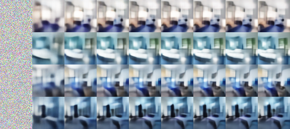
Infusion training (Bordes et al., 2016) trains a Markov chain to gradually converge to the data distribution $p_{data}$. Formally, training starts with some initial random noise $x^{(0)}\sim p^{(0)}$, and goes through the following two steps iteratively

1)Infusion: A new ”latent state” $z^{(t)}$ is generated by taking the previous reconstruction $x^{(t)}$, and adding some pixels from a ground truth data point $x_{data}$.

2)Reconstruction: The decoding model attempts the next reconstruction $p^{(t)}(x^{(t+1)}|z^{(t)})$ by maximizing $\log p^{(t)}(x_{data}|z^{(t)})$. The superscript $t$ indicates that this can be a different distribution for each step $t$, leading to a non-homogeneous Markov chain.

To draw new samples at test time, we directly sample from the Markov chain

initializing from random noise. This idea is illustrated in Figure 3. Note that we refer to the resulting image after infusion $z^{(t)}$ as a ”latent state” because it plays the same role as a VAE latent state. We can interpret the probability of obtaining $z^{(t)}$ by the above iterative procedure as an inference distribution $q(z^{(t)}|x)$. In contrast with VAEs, the inference distribution used in infusion training is manually specified by the ”infusion” process. By adding more true pixels and making $z^{(t)}$ increasingly informative about $x$, for sufficiently large $t$ the ”latent code” $z^{(t)}$ will become informative enough to have a simple posterior $q(x|z^{(t)})$ that is highly concentrated on $x$. Such a posterior can be well approximated by simple unimodal conditionals $\mathcal{P}$, such as Gaussian distributions.

Inspired by this idea, we propose the model shown in Figure 3 which we will call a sequential VAE. Each step is a VAE, except the decoder $p_{\theta}(x|z)$ is now also conditioned on the previous reconstruction outcome. We go through the following two steps iteratively during training:

1) Inference: An inference distribution $q_{\phi_{t}}(z^{(t)}|x)$ maps a ground truth data point $x_{data}$ to a latent code.

2) Reconstruction: A generative distribution (decoder) that takes as input a sample from the previous step $x^{(t-1)}$ and latent code $z^{(t)}$ to generate a new sample $p_{\theta_{t}}(x^{(t)}|z^{(t)},x^{(t-1)})$. When $t=0$, we do not condition on previous samples.

The model is jointly trained by maximizing the VAE criteria for each time step respectively.

For experiments in this section we use ELBO regularization (Kingma & Welling, 2013) $R(q_{\phi_{t}})=KL(q_{\phi_{t}}(z^{(t)}|x_{data})||p(z^{(t)}))$ where $p(z^{(t)})$ is a simple fixed prior such as white Gaussian.

To generate samples during test time, for each step we perform ancestral sampling $p(z^{(t)})p_{\theta_{t}}(x^{(t)}|z^{(t)},x^{(t-1)})$. Details about implementation is described in the Appendix.

The idea is that the more latent code we add, the more we know about $x$, making the posterior $q(x|z^{(0:t)})$ simpler as $t$ becomes larger. In particular, we can show this formally for 2-norm loss as in Section 3.1.

Therefore increasing the latent code size in expectation does not increase variance. By the connection we established between variance of the posterior and blurriness of the samples, this should lead to sharper samples. We show this experimentally in Figure 4¹¹ 1 Code is available at https://github.com/ShengjiaZhao/Sequen
tial-Variational-Autoencoder, where we evaluate our model on CelebA and LSUN. In particular we can generate sharp LSUN images based only on 2-norm loss in pixel space, something previously considered to be difficult for VAE models. Details about architecture and training are in the Appendix.

Sequential generation is a general scheme under which many different models are possible. It encompasses infusion training as a special case, but many different variants are possible. This idea has great potential for improving auto-encoding models based on simple, unimodal $\mathcal{P}$ families.

References

- Arjovsky et al. (2017) Arjovsky, M., Chintala, S., and Bottou, L. Wasserstein GAN. ArXiv e-prints, January 2017.
- Bachman (2016) Bachman, Philip. An architecture for deep, hierarchical generative models. In Advances In Neural Information Processing Systems, pp. 4826–4834, 2016.
- Bordes et al. (2016) Bordes, Florian, Honari, Sina, and Vincent, Pascal. Learning to generate samples from noise through infusion training. https://openreview.net/pdf?id=BJAFbaolg, 2016.
- Bowman et al. (2015) Bowman, Samuel R., Vilnis, Luke, Vinyals, Oriol, Dai, Andrew M., Józefowicz, Rafal, and Bengio, Samy. Generating sentences from a continuous space. CoRR, abs/1511.06349, 2015. URL http://arxiv.org/abs/1511.06349.
- Burda et al. (2015) Burda, Yuri, Grosse, Roger, and Salakhutdinov, Ruslan. Importance weighted autoencoders. arXiv preprint arXiv:1509.00519, 2015.
- Chen et al. (2016) Chen, Xi, Kingma, Diederik P, Salimans, Tim, Duan, Yan, Dhariwal, Prafulla, Schulman, John, Sutskever, Ilya, and Abbeel, Pieter. Variational lossy autoencoder. arXiv preprint arXiv:1611.02731, 2016.
- Chung et al. (2015) Chung, Junyoung, Kastner, Kyle, Dinh, Laurent, Goel, Kratarth, Courville, Aaron C., and Bengio, Yoshua. A recurrent latent variable model for sequential data. CoRR, abs/1506.02216, 2015. URL http://arxiv.org/abs/1506.02216.
- Dosovitskiy & Brox (2016) Dosovitskiy, Alexey and Brox, Thomas. Generating images with perceptual similarity metrics based on deep networks. CoRR, abs/1602.02644, 2016. URL http://arxiv.org/abs/1602.02644.
- Goodfellow et al. (2014) Goodfellow, Ian, Pouget-Abadie, Jean, Mirza, Mehdi, Xu, Bing, Warde-Farley, David, Ozair, Sherjil, Courville, Aaron, and Bengio, Yoshua. Generative adversarial nets. In Advances in Neural Information Processing Systems, pp. 2672–2680, 2014.
- Gulrajani et al. (2016) Gulrajani, Ishaan, Kumar, Kundan, Ahmed, Faruk, Taiga, Adrien Ali, Visin, Francesco, Vázquez, David, and Courville, Aaron C. Pixelvae: A latent variable model for natural images. CoRR, abs/1611.05013, 2016. URL http://arxiv.org/abs/1611.05013.
- Jimenez Rezende et al. (2014) Jimenez Rezende, D., Mohamed, S., and Wierstra, D. Stochastic Backpropagation and Approximate Inference in Deep Generative Models. ArXiv e-prints, January 2014.
- Kaae Sønderby et al. (2016) Kaae Sønderby, C., Raiko, T., Maaløe, L., Kaae Sønderby, S., and Winther, O. Ladder Variational Autoencoders. ArXiv e-prints, February 2016.
- Kingma & Welling (2013) Kingma, D. P and Welling, M. Auto-Encoding Variational Bayes. ArXiv e-prints, December 2013.
- Kingma et al. (2016) Kingma, Diederik P, Salimans, Tim, and Welling, Max. Improving variational inference with inverse autoregressive flow. arXiv preprint arXiv:1606.04934, 2016.
- Lamb et al. (2016) Lamb, Alex, Dumoulin, Vincent, and Courville, Aaron. Discriminative regularization for generative models. arXiv preprint arXiv:1602.03220, 2016.
- Larsen et al. (2015) Larsen, Anders Boesen Lindbo, Sønderby, Søren Kaae, and Winther, Ole. Autoencoding beyond pixels using a learned similarity metric. arXiv preprint arXiv:1512.09300, 2015.
- Nowozin et al. (2016) Nowozin, Sebastian, Cseke, Botond, and Tomioka, Ryota. f-gan: Training generative neural samplers using variational divergence minimization. In Advances in Neural Information Processing Systems, pp. 271–279, 2016.
- Radford et al. (2015) Radford, Alec, Metz, Luke, and Chintala, Soumith. Unsupervised representation learning with deep convolutional generative adversarial networks. arXiv preprint arXiv:1511.06434, 2015.
- Salimans et al. (2017) Salimans, Tim, Karpathy, Andrej, Chen, Xi, and Kingma, Diederik P. Pixelcnn++: Improving the pixelcnn with discretized logistic mixture likelihood and other modifications. arXiv preprint arXiv:1701.05517, 2017.
- van den Oord et al. (2016a) van den Oord, Aaron, Kalchbrenner, Nal, Espeholt, Lasse, Vinyals, Oriol, Graves, Alex, et al. Conditional image generation with pixelcnn decoders. In Advances in Neural Information Processing Systems, pp. 4790–4798, 2016a.
- van den Oord et al. (2016b) van den Oord, Aäron, Kalchbrenner, Nal, and Kavukcuoglu, Koray. Pixel recurrent neural networks. CoRR, abs/1601.06759, 2016b. URL http://arxiv.org/abs/1601.06759.
Appendix A Additional Results
A.1 Comparison to Adversarial Training
Adversarial training (Goodfellow et al., 2014) has shown great promise in generating high quality samples. Analysis in this paper points to a possible explanation of its relative success in complex natural image datasets compared to variational autoencoders. In Proposition 1 we pointed out that if then the model has no incentive to take advantage of this representation capacity by mapping them to different members of . This is the key reason why a simple family require a almost ”lossless” , and failure to satisfy this condition leads to fuzziness and other problems.
However adversarial training does not suffer from this limitation. In fact even without inference, adversarial training can map different latent code to different members of . This is because for adversarial training we are not using to approximate . Instead we are selecting a member of whose support is covered by the support of real data. Intuitively, we would like to generate any real looking samples, and not a particular set.
Therefore we expect adversarial training to have advantage over VAE when is expected to be complex, and is simple. However we showed in this paper that models with complex , but carefully designed to avoid the information preference property also show great promise.
A.2 Failure Modes for Factorized Discrete Family
When is the family of factorized discrete distribution , where each is a discrete distribution on the -th dimension. We obtain similar results
Proposition 6.
The optimal solution to when is the family of discrete distribution for a given is for all ,
and for each the best achievable error is the pixel-wise negative entropy
This shows us that for discrete distributions, mismatch between and manifests in a different way: by generating excessively noisy output where each pixel is independently sampled.
A.3 Estimating Mutual Information
Because
We can estimate mutual information by obtaining samples , and
This gives us good estimates unless the mutual information is large because the above estimation is upper bounded by
This problem is not specific to our method of approximation. In fact, suppose the dataset has samples, then true mutual information under the empirical data distribution is also upper bounded by
Appendix B Proofs
Proof of Proposition 123.
For any , because
When is a sufficiently large family, there must be a so that for all , . Therefore