Non-Concave Network Utility Maximization in Connectionless Networks: A Fully Distributed Traffic Allocation Algorithm Note:  This work was partially supported by NSF grants CNS-1329422, CMMI-1635106, FCC-1629625, NNSF of China grants 61673026 and the China Scholarship Council.

Applications and services supported by modern communication networks have diverse requirements, e.g., high throughput and low latency. Traffic engineering (TE) has long been used to optimize the utilization of the limited network resources so that such requirements are fulfilled. This entails developing data rate allocation algorithms and congestion control protocols capable of maximizing a given network utility subject to network resource constraints [1]. Many problems of recent interest arising in diverse fields can be cast as an optimization problem, and network utility maximization (NUM) is no different.

In large-scale networks, the size of the optimization problems rapidly increases as the number of nodes and links increase. This stimulates the necessity of developing decentralized control algorithms capable of decomposing the high-dimensional problem into separate moderate-size subproblems that can be solved independently and locally at various network nodes. The main idea behind such decentralized control algorithms is to distribute the computations required for the solution of the optimization problem among various nodes [2]-[4]. This approach exploits local information available at each node. Nevertheless, information exchange among different nodes is inevitable since distinct data flows share the same network resources. Therefore, distributed optimization approaches not only aim at decomposing the problem, but also minimizing the communication overhead.

In the benchmark work by Kelly et. al. [1], the optimization of the utility of a large-scale broadband network with limited bandwidth resources is considered. The authors propose two classes of rate control algorithms by casting the NUM problem in both primal and dual forms. In [2], a family of decentralized sending rate control laws are proposed to steer the traffic allocation to an optimal operating point while avoiding congestion. A non-linear control theoretic approach is employed in [3] to derive adaptation laws that enable each node to independently distribute its traffic optimally among any given set of next hops. More recently, reference [4] considers the NUM, derives its dual problem, and uses a distributed gradient-based approach for its solution. A similar approach appears in [5]. In spite of the existence of a relatively dense literature on NUM, most available results consider only the optimization of concave utility functions. However, it has been shown that the reward experienced by the users of real-time applications, such as video and audio streaming, cannot be accurately modeled using concave functions. Reference [6] shows that the video quality perceived by users on a mobile device is a non-decreasing and step-like function with respect to the data rate, because users have almost similar quality of experience on $3$ Mbps and $1$ Mbps [6]. This observation motivates considering the optimization of non-concave network utility functions, which constitutes a main focus of this paper.

Non-concave NUM is a non-convex optimization problem; hence, it is difficult to solve. Nevertheless, there exist some attempts in the literature for deriving algorithms that provide near-optimal solutions. Reference [7] develops a centralized algorithm that solves the NUM problem with polynomial utilities. Reference [8] determines the conditions under which the standard distributed dual-based algorithm can still converge to the global optimal solution with non-concave utilities.

This paper develops a distributed iterative algorithm for the optimization of a generalized class of non-concave network utility functions that capture a wide variety of real-world applications. In particular, we focus on connectionless networks, where each node is required to distribute its traffic among a set of next hops without prior arrangement so that the network utility is maximized. We handle the challenge posed by the non-convexity of the optimization problem by developing a sequence of convex relaxations whose solution converges to that of the original problem. We use results on polynomial optimization and moment sequences to derive the convex relaxations [9, 10]. Furthermore, we propose an iterative primal-dual algorithm [11] that enables each node to distribute its traffic among the set of next hops. We emphasize on the distributed nature of the algorithm, where each node uses its local information and need not communicate with other nodes except its direct neighbors.

Throughout this paper, the traffic flows are assumed to be described by a fluid flow model, and the only resource constraint taken into account is link bandwidth. In the remainder of this paper, call and flow will be used interchangeably.

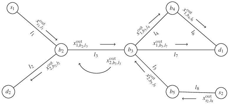
Let $\mathcal{N}$ denote the set of nodes in the network, and $\mathcal{L}\subset\mathcal{N}\times\mathcal{N}$ denote the set of links connecting particular pairs of nodes. We assume that each link $l\in\mathcal{L}$ has a finite capacity $c_{l}>0$. Moreover, let $\mathcal{S}\triangleq\{s_{1},s_{2},\ldots,s_{n}\}$ and $\mathcal{D}\triangleq\{d_{1},d_{2},\ldots,d_{n}\}$ denote respectively the set of source nodes and the set of destination nodes contained in $\mathcal{N}$ such that $\mathcal{S}\cap\mathcal{D}=\emptyset$. The intended destination for each source node $s_{i}$ is $d_{i}$ for $i\in\mathcal{I}\triangleq\{1,\ldots,n\}$, i.e., without loss of generality, we assume that there is a one-to-one correspondence between $\mathcal{S}$ and $\mathcal{D}$, and $\mathcal{I}$ denotes the set of different flow (call) types in the network. Given source node $s\in\mathcal{S}$, let $\mathcal{L}_{s}$ denote the set of links connected to it. Let the sending data rate through link $l\in\mathcal{L}_{s}$ be $x_{s,l}^{\text{out}}$, and all such sending data rates be $\mathbf{x}_{s}^{\text{out}}\triangleq[x_{s,l}^{\text{out}}]_{l\in\mathcal{L}_{s}}$. We define the aggregate sending data rate of $s\in\mathcal{S}$ be denoted by $r_{s}\triangleq\sum_{l\in\mathcal{L}_{s}}x_{s,l}^{\text{out}}$. Also, let $\mathcal{B}\triangleq\mathcal{N}\setminus(\mathcal{S}\cup\mathcal{D})=\{b_{1},b_{2},\ldots,b_{m}\}$ denote the set of forwarding nodes contained in $\mathcal{N}$. Given $b\in\mathcal{B}$, let $\mathcal{I}_{b}$ be the set of flows visiting node $b$, and $\mathcal{L}_{b}\subseteq\mathcal{L}$ denote the set of links connected to it. Suppose $\mathcal{L}_{b,i}^{\text{out}}\subseteq\mathcal{L}_{b}$ denote the set of outgoing links from $b$ associated with calls (flows) of type $i\in\mathcal{I}_{b}$. Similarly, let $\mathcal{L}_{b,i}^{\text{in}}\subset\mathcal{L}_{b}$ denote the set of incoming links to $b$ associated with calls (flows) of type $i\in\mathcal{I}_{b}$. Furthermore, given $b\in\mathcal{B}$, for each $i\in\mathcal{I}_{b}$ and $l\in\mathcal{L}_{b,i}^{\text{out}}$, let $x_{i,b,l}^{\text{out}}$ denote the data rate of call type $i\in\mathcal{I}_{b}$, associated with $s_{i}$ and $d_{i}$, forwarded from node $b$ through link $l\in\mathcal{L}_{b,i}^{\text{out}}$. The above notation is exemplified in Fig. 1 for the case of allocating flows associated with two source nodes, $s_{1}$ and $s_{2}$, and two destination nodes, $d_{1}$ and $d_{2}$.

Given $b\in\mathcal{B}$ and $l\in\mathcal{L}_{b}$, let $\mathcal{I}_{b,l}^{\text{in}}\subset\mathcal{I}$ be the set of call types forwarded to node $b$ through link $l$, and $\mathcal{I}_{b,l}^{\text{out}}\subseteq\mathcal{I}_{b}$ be the set of call types forwarded from node $b$ through link $l$. Moreover, given node $b\in\mathcal{B}$ and link $l\in\mathcal{L}_{b}$, let $e_{l}(b)$ denote the adjacent node to $b$ through link $l$. We summarize all the notation for the communication network in Table I for the convenience of the reader.

Now, given node $b\in\mathcal{B}$, let the vector containing all flow rates departing from node $b$ through link $l\in\mathcal{L}_{b}$ be denoted by $\mathbf{x}_{b,l}^{\text{out}}\triangleq[x_{i,b,l}^{\text{out}}]_{i\in\mathcal{I}_{b,l}^{\text{out}}}\in\text{R}_{+}^{|\mathcal{I}_{b,l}^{\text{out}}|}$, where $|.|$ denotes the cardinality of a set.

Given node $b\in\mathcal{B}$ and $l\in\mathcal{L}_{b}$, let $\mathbf{1}_{b,l}\in\text{R}^{1\times|\mathcal{I}_{b,l}^{\text{out}}|}$ be the row vector with all elements equal to $1$. In a similar way, let $\delta_{b,l}\in\text{R}^{1\times|\mathcal{I}_{b,l}^{\text{in}}|}$ be the row vector with all elements equal to $1$ if link $l$ is bidirectional, and $0$ otherwise.

Also, let $\|.\|$ denote the Euclidean norm. Given a convex set $\mathcal{A}$, let $\mathit{I}_{\mathcal{A}}(.)$ denote the indicator function of $\mathcal{A}$, i.e., $\mathit{I}_{\mathcal{A}}(\omega)=0$ for $\omega\in\mathcal{A}$ and equal to $+\infty$ otherwise, and let $\mathit{P}_{\mathcal{A}}(\omega)\triangleq\text{argmin}\{\|\upsilon-\omega\|:\upsilon\in\mathcal{A}\}$ denote the projection onto $\mathcal{A}$. Given a closed convex set $\mathcal{A}$, we define the distance function as $d_{\mathcal{A}}(\omega)\triangleq\|\mathit{P}_{\mathcal{A}}(\omega)-\omega\|$. Also, $\mathbf{I}_{n}$ is the $n\times n$ identity matrix.

Consider a communication network consisting of a set of source nodes $\mathcal{S}$. Each source node $s\in\mathcal{S}$ has a local utility function $U_{s}(r_{s}):\mathrm{R}_{+}\to\mathrm{R}_{+}$ of its sending data rate $r_{s}$. For a fixed order $\ell>0$, the utility function is defined as a general non-concave polynomial-like function in the form

This particular form of objective functions is so flexible that it can be used to approximate a wide variety of functions arising in practical applications such as step functions for the video streaming case [5].

The objective of this paper is to design a data rate allocation algorithm for the communication network such that the utilization of resources is maximized, while satisfying the network resource constraints. The network resource constraints considered in this paper include link capacity constraints, Minimum Rate Guaranteed and Upper Bounded Rate Service (MRGUBRS) requirements, and flow conservation constraints through nodes.

More precisely, for any link $l\in\mathcal{L}$, the aggregated flows going through this link should not exceed the link capacity. For example, in Fig. 1, the bidirectional link $l_{3}$ is shared by flows belonging to two source nodes. The data rates $x_{1,b_{2},l_{3}}^{\text{out}}$ and $x_{2,b_{3},l_{3}}^{\text{out}}$ going through this link should satisfy that

For the unidirectional link $l_{2}$, node $b_{2}$ forwards data rate $x_{2,b_{2},l_{2}}^{\text{out}}$ through this link. Then, $x_{2,b_{2},l_{2}}^{\text{out}}$ is upper bounded by $c_{l_{2}}$.

Given flows of type $i\in\mathcal{I}$, recall that flows of type $i\in\mathcal{I}$ is associated with source/destination pairs $s_{i}/d_{i}$. For fixed link $l\in\mathcal{L}_{s_{i}}$, the corresponding data rate $x_{i,l}^{\text{out}}$ is determined at source node $s_{i}\in\mathcal{S}$ and multiple paths are available for transporting these flows. More precisely, each node on these paths divide incoming traffic into available links by striving to conserve the flows belonging to each source node (i.e., aims at no losses) and to avoid link congestion. In Fig. 1, node $b_{3}$ tries to satisfy

Finally, flows belonging to each source node $s\in\mathcal{S}$ is assumed to be of the MRGUBS category, i.e., for some $0<\xi_{s}<\zeta_{s}$ and $s\in\mathcal{S}$,

Now, considering the above constrains and assumptions, we can formulate the problem of optimal traffic allocation as follows:

subject to the network capacity constraints ¹¹ 1 Note that the formulation in this paper allows for the existence of bidirectional links.

the flow conservation constraints at each node

the non-negativity of forwarded data rates constraints

and the MRGUBS requirements

where the set $\mathcal{X}_{s}$ is defined as

Most literature in the context of NUM considers maximizing concave diminishing functions. However, modern communication networks are dominated by various inelastic applications, such as internet video and audio streaming. Users’ satisfaction for these applications cannot be modeled with concave functions. It is better to be described as non-concave functions. For instance, the utility for voice applications is a sigmoidal function [7]. Thus, we consider users’ perceived qualification of Cost of Service (CoS) and model the utility function as a general class of non-concave polynomial functions. Moreover, the challenges of attempting to solve the resulting traffic allocation problem (5) are two-fold. First, the optimization problem obviously constitutes a non-convex problem since its objective function is non-concave. Second, global information on fast timescale events, as required in the above formulation, is not generally available. The latter fact stimulates the necessity of developing a distributed algorithm that converges to the optimal data rate allocation of the non-convex NUM problem.

In this section, we present our approach used to overcome the challenges opposed by the non-convexity of the optimization problem. In particular, we first present a convex relaxation to the non-convex NUM problem (5). This convex relaxation is chosen from a hierarchy of optimization problems whose optimal value converges to the optimal value of problem (5) as the number of moments tends to infinity. For solving the convex relaxation problem, we propose a distributed primal-dual algorithm (DPDA), which enables all nodes to update their data rate allocation solely using immediate local information. A salient feature of the proposed algorithm is that the iterate sequence converges to the optimal solution at a $O(1/K)$ rate, where $K$ is the iteration counter, with a bounded optimality.

In this section, we present some simulation results which exemplify the behavior of the proposed algorithm, i.e., Algorithm DPDA. The simulations show that the final data rate allocation results in a value of the utility function barely distinguishable from the optimal one.

We consider the network model shown in Fig. 2, where we also show all the links’ bandwidths, and source-destination pairs. The network model allows for multiple paths available for flows belonging to each source node. We consider a total of $8$ different combinations of source/destination nodes. Moreover, we list the prescribed next hops for all forwarding nodes $b_{i},\ i=1,\ldots,8$, in Table II. For example, the upper left cell means that node $b_{1}$ forwards the data of source $s_{1}$ to nodes $b_{2}$ and $b_{7}$.

The objective throughout the simulation is to maximize the sum utility of source nodes, where source $s_{i},\ i=1,\ldots,8$, has the utility function given by

$U_{s_{i}}(r_{s_{i}})$ is a step-like non-concave polynomial-like function. We consider to optimize a step-like non-concave function, because it is more likely to describe the video quality perceived by a user in a video streaming application [5]. Moreover, we obtain the resource constraints information from Fig. 2 and Table. II, and impose the lower and upper bounds on the aggregate data rate of each user as $\xi_{s_{i}}=0$ and $\zeta_{s_{i}}=10,\ i=1,\ldots,8$, respectively.

Given the network topology shown in Fig. 2, we choose the step-size parameters to satisfy the convergence condition set forth by Theorem $2$. All step-size parameters are chosen locally using local information. Fig. 3 shows the performance of Algorithm DPDA for these step-size parameters. It can be seen that the utility function converges to the optimal one, which is obtained by using Genetic Algorithm while assuming the availability of global information. Although all the computations of DPDA are performed locally at each node, it attains almost the same network utility obtained by a centralized optimization algorithm. This implies that the iterate sequence of Algorithm DPDA can indeed converge to the optimal traffic allocation.

Fig. 4 shows the representative data rate trajectories for MRGUBS flows belonging to source nodes $s_{3}$ and $s_{4}$. Both data rate sequences are generated by DPDA. It can be seen from Fig. 4 that the MRGUBS requirements are satisfied.

In this paper, we proposed a distributed traffic allocation algorithm, i.e., DPDA, to allow distributed optimal traffic engineering in a connectionless autonomous network. DPDA is distributed and converges at a $\mathit{O}(1/K)$ rate, where $K$ is the number of iterations. Moreover, numerical simulation results showed that the behavior of DPDA mimics the optimal traffic distribution.

The results presented in this paper are just the first step towards the implementation of an optimal fast distributed algorithm for traffic engineering. There are many issues that need further consideration. In particular, efforts should be put on testing the implementation in large-scale network settings.

In this Appendix, we include some results from real analysis theory and the main steps of proving Proposition $1$.

The constrains set of convex relaxation (6) consists of local constraints, e.g., capacity constraints and global constraints, e.g., flow conservation constraints through nodes. The existence of global constraints renders difficulty for us to solve problem (6) in a distributed fashion. However, the primal-dual method, proposed by Chambolle and Pock in [14] for solving convex-concave saddle point problems makes it possible. This algorithm can be adapted to solve the multi-agent consensus optimization problem as discussed in [11]. We also use the distributed primal-dual algorithm in [11] to solve our traffic allocation problem (6). This Appendix aims at developing the distributed algorithm that converges to the solution of (6).

The optimization problem (6) can be compactly stated as

REFERENCES

• [1] F. P. Frank, A. K. Maulloo and D. K. H. Tan, Rate control for communication networks: shadow prices, proportional fairness and stability, Journal of the Operational Research society, Springer, vol. 49, no. 3, pp. 237–252, 1998.
• [2] C. M. Lagoa, H. Che and B. A Movsichoff, Adaptive control algorithm for dencentralized optimal traffic engineering in the Internet, IEEE/ACM Transactions on Networking, vol. 12, no. 3, pp. 415–428, June 2004.
• [3] B. A. Movsichoff, A. Bernardo, C. M. Lagoa and H. Che, Decentralized optimal traffic engineering in connectionless networks, IEEE Journal on Selected Areas in Communications, vol. 23, no. 2, pp. 293–303, 2005.
• [4] A. Beck, A.  Nedic, A. Ozdaglar and M. Teboulle, Optimal distributed gradient methods for network resource allocation problems, Submitted for publication, 2013.
• [5] E. Nekouei, G. Nair and T.  Alpcan, Convergence analysis of quantized primal-dual algorithm in quadratic network utility maximization problems, IEEE Conference on Decision and Control CDC, pp. 2655–2660, 2015.
• [6] X. Q. Yin, A. Jindal, V. Sekar and B. Sinopoli, A control-theoretic approach for dynamic adaptive video streaming over HTTP, SIGCOMM, London, United Kingdom, pp. 325–338, August 2015.
• [7] M. Fazel and M. Chiang, Network utility maximization with nonconcave utilities using sum-of-squares method, Proceedings of the 44th IEEE Conference on Decision and Control, 2005, pp. 1867–1874.
• [8] P. Hande, S. Y. Zhang and M. Chiang, Distributed rate allocation for inelastic flows, IEEE/ACM Transactions on Networking, vol. 15, no. 6, pp. 1240–1253, 2007.
• [9] J. B. Lasserre, Global optimization with polynomials and the problem of moments, SIAM Journal on Optimization, vol. 11, no. 3, pp. 796–817, 2001.
• [10] M. Laurent, Sums of squares, moment matrices and optimization over polynomials, Emerging applications of algebraic geometry, Springer New York, 2009: 157–270.
• [11] N. S. Aybat and E. F. Hamedani, A primal-dual method for conic constrained distributed optimization problems, Advances in Neural Information Processing Systems 29, edited by D. D. Lee and M. Sugiyama and U. V. Luxburg and I. Guyon and R. Garnett, Curran Associates, Inc., pp. 5049–5057, 2016, http://papers.nips.cc/paper/6242-a-primal-dual-method-for-conic-constrained-distributed-optimization-problems.pd.
• [12] N. Ozay, C. M. Lagoa and M. Sznaier, Set membership identification of switched linear systems with known number of subsystems, Automatica, vol. 51, pp. 180–191, 2015.
• [13] M. G. krein and A. A. Nudelman, The markov moment problem and extremal problems, volume 50 of translations of mathematical monographs, American Mathematical Society, Providence, Rhode Island, 1977.
• [14] A. Chambolle and T. Pock, On the ergodic convergence rates of a first-order primal-dual algorithm, Mathematical Programming, Springer, 2015, pp. 1–35.
• [15] G. H. Golub and C. F. Van Loan, Matrix Computations (3rd Ed.), Johns Hopkins University Press, Baltimore, MD, USA, 1996.