Elementary Yet Precise Worst-case Analysis of MergeSort
A short version (SV) of a manuscript
intended for future publication
Note: ©2017 Marek A. Suchenek.
Abstract
The full version of this paper offers two elementary yet precise derivations of an exact formula
for the maximum number of comparisons of keys performed by on an -element array. The first of the two, due to its structural regularity, is well worth carefully studying in its own right.
Close smooth bounds on are derived. It seems interesting that is linear between the points and it linearly interpolates its own lower bound between these points.
The manuscript (MS) of the full version of this paper, dated January 20, 2017, can be found at:
http://csc.csudh.edu/suchenek/Papers/Analysis_of_MergeSort.pdf
Keywords:
MergeSort , sorting , worst case.2010 MSC
68W40 Analysis of algorithmsACM Computing Classification
Theory of computation: Design and analysis of algorithms: Data structures design and analysis: Sorting and searching
Mathematics of computing: Discrete mathematics: Graph theory: Trees
Mathematics of computing: Continuous mathematics: Calculus
ACM classes: F.2.2; G.2.0; G.2.1; G.2.2
1 Introduction
is one of the fundamental sorting algorithms that is being taught in undergraduate Computer Science curricula across the U.S. and elsewhere. Its worst-case performance, measured by the number of comparisons of keys performed while sorting them, is optimal for the class of algorithms that sort inductively11 1 Inductive sorting of keys sorts a set of of those keys first, and then “sorts-in” the remaining -th key. by comparisons of keys.22 2 In its standard form analyzed in this paper, is not an inductive sorting algorithm. However, its worst-case performance, measured by the number of comparisons of keys performed while sorting them, is equal to the worst-case performance of the binary insertion sort first described by Steinhaus in [5] that is worst-case optimal in the class of inductive sorting algorithms that sort by comparisons of keys; see [3] page 186. Historically, it33 3 A bottom-up version of it, invented by John Neumann. was the first sorting algorithm to run in time44 4 In the worst case..
So it seems only fitting to provide an exact formula for ’s worst-case performance and derive it precisely. Unfortunately, many otherwise decent texts offer unnecessarily imprecise55 5 Notable exceptions in this category are [2] and [4] that derive almost exact formulas, but see Section 8 page 8 for a brief critique of the results and their proofs offered there. variants of it, and some with quite convoluted, incomplete, or incorrect proofs. Due to these imperfections, the fact that the worst-case performance of is the same as that of another benchmark sorting algorithm, the binary insertion sort of [5], has remained unnoticed66 6 Even in [3]..
In this paper, I present two outlines77 7 The detailed derivations can be found in [9]. of elementary yet precise and complete derivations of an exact formula
for the maximum number 88 8 Elementary derivation of an exact formula for the best-case performance of , measured by the number of comparisons of keys performed while sorting them, has been done in [8]; see Section 9 page 9 of this paper. of comparisons of keys performed by on an -element array. The first of the two, due to its structural regularity, is well worth carefully studying in its own right.
Unlike some other basic sorting algorithms99 9 For instance, ; see [7] for a complete analysis of its worst-case behavior. that run in time, exhibits a remarkably regular1010 10 As revealed by Theorem 5.2, page 5.2. worst-case behavior, the elegant simplicity of which has been mostly lost on its rough analyses. In particular, is linear1111 11 See Figure 4 page 4. between the points and it linearly interpolates its own lower bound 1212 12 Given by the left-hand side of the inequality (12) page 12. between these points.
What follows is a short version (SV) of a manuscript dated January 20, 2017, of the full version version [9] of this paper that has been posted at:
http://csc.csudh.edu/suchenek/Papers/Analysis_of_MergeSort.pdf
2 Some Math prerequisites
A manuscript of the full version [9] of this paper contains a clever derivation of a well-known1414 14 See [3]. closed-form formula for . It proves insightful in my worst-case analysis of as its right-hand side will occur on page 5 in the fundamental equality (5) and serve as an instrument to derive the respective exact formula for ’s worst-case behavior.
Lemma 2.1.
For every integer ,
| (1) |
Proof in [9].
From this one can easily conclude that:
Corollary 2.2.
For every integer ,
| (2) |
3 and its worst-case behavior
A call to inherits an -element array of integers and sorts it non-decreasingly, following the steps described below.
Algorithm 3.1.
To sort an -element array do:
- 1.
If then return to the caller,
- 2.
If then
- (a)
pass the first elements of to a recursive call to ,
- (b)
pass the last elements of to another recursive call to ,
- (c)
linearly merge, by means of a call to , the non-decreasingly sorted arrays that were returned from those calls onto one non-decreasingly sorted array ,
- (d)
return to the caller.
- (a)


A typical measure of the running time of is the number of comparisons of keys, which for brevity I call comps, that it performs while sorting array .
Definition 3.2.
The worst-case running time
of is defined as the maximum number of comps it performs while sorting an array of distinct1616 16 This assumption is superfluous for the purpose of worst-case analysis as the mere presence of duplicates does not force to perform more comps. elements.
Clearly, if then . From this point on, I am going to assume that .1717 17 This assumption turns out handy while using expression .
Since no comps are performed outside , can be computed as the sum of numbers of comps performed by all calls to during the execution of . The following classic results will be useful in my analysis.
Theorem 3.3.
The maximum number of comps performed by on two sorted list of total number of elements is .
Moreover, if the difference between the lengths of merged list is not larger than 1 then no algorithm that merges sorted lists by means of comps beats in the worst case, that is, has a lower than maximum number of comps.1818 18 Proof in [3], Sec. 5.3.2 page 198; the worst-case optimality of ( comps) was generalized in [6] over lists of lengths and , with , that satisfy . This fact makes optimal in the intersection of the class of sorting algorithms that sort by merging two sorted lists of lengths’ difference not larger than 1 1919 19 Or, by virtue of the above-quoted result from [6], with the difference not larger than the half of the length of the shorter list plus 1. with the class of sorting algorithms that sort by comps.
4 An easy yet precise derivation of
is a recursive algorithm. If then it spurs a cascade of two or more recursive calls to itself. A rudimentary analysis of the respective recursion tree , shown on Figure 2, yields a neat derivation of the exact formula for the maximum number of comps that performs on an -element array.

The idea behind the derivation is strikingly simple. It is based on the observation2020 20 Which I prove in [9] as Theorem 4.6, page 14. that for every , the maximum number of comps performed at each level2121 21 Empty or not. of is given by this neat formula:2222 22 It is a simplification of formulas used in derivation presented in [2] and discussed in Section 8 page 8; in particular, it does not refer to the depth of the decision tree .
| (3) |
Since
| (4) |
the Corollary 2.2 will allow me to conclude from (3) and (4) the main result of this paper2323 23 This is how I have been deriving it in my undergraduate Analysis of Algorithms class for some 15 years or so, now.:
| (5) |
The missing details2424 24 Which I did not show in my Analysis of Algorithms class. in the above sketch are in [9]. Naturally, their only purpose is to prove the equality (3) for all , as the rest, shown in (5), easily follows from it. In particular, we get:
The Main Theorem 4.1.
The number of comparisons of keys that performs in the worst case while sorting an -element array is
| (6) |
Proof in [9].
From that we can conclude a usual rough characterization of :
and
Therefore,
The occurrence of in (6) allows to conclude that is exactly equal2525 25 [3] contains no mention of that fact. to the number of comparisons of keys that the binary insertion sort, considered by H. Steinhaus in [5] and analyzed in [3], performs in the worst case. Since the binary insertion sort is known to be worst-case optimal2626 26 With respect to the number of comparisons of keys performed. in the class of algorithms that perform incremental sorting, is worst-case optimal in that class2727 27 Although it is not a member of that class., too. From this and from the observation at the end of Section 3, page 3, I conclude that no algorithm that sorts by merging two sorted lists and only by means of comps is worst-case optimal in the class of algorithms that sort by means of comps as it must perform 8 comps in the worst case while sorting 5 elements2828 28 They can be split in two: 1 plus 4, and follow the binary insertion sort, or 2 plus 3, and follow ., while one can sort 5 elements by means of comps with no more than 7 comps.
5 Close smooth bounds on
Our formula for contains a function ceiling that is harder to analyze than arithmetic functions and their inverses. In this Section, I outline a derivation of close lower and upper bounds on that are expressible by simple arithmetic formulas. I show that these bounds are the closest to in the class of functions of the form , where is a real constant. The detailed derivation and missing proofs can be found in [9].
Using the function (analyzed briefly in [3] and [7]), a form of which is shown on Figure 3, given by:
| (7) |
one can conclude2929 29 See [7], Thm. 12.2 p. 94 for a proof. that, for every ,
| (8) |
which yields
| (9) |
Property 5.1.
Function given by (7) is a continuous function of on the set of reals . It assumes the minimum for every and the maximum
| (10) |
for every
| (11) |
and only such . The function restricted to integers never reaches the value . However, is the supremum of restricted to integers.
Proof in [9].
Characterization (9) and Property 5.1 yield close smooth bounds of . They are both of the form and they sandwich tightly between each other. If one sees as an infinite polygon3131 31 Which it is., its lower bound circumscribes it and its upper bound inscribes it.
Theorem 5.2.
is a continuous concave function, linear between the points , that for every satisfies this inequality:
| (12) |
with the left becoming for every and the right becoming for every , and only for such . Moreover, the graph of is tangent to the graph of at the points , and only at such points.
Proof in [9].
The bounds given by (12) are really close3232 32 The distance between them is less than for any positive integer . to the exact value of , as it is shown on Figure 4 page 4. The exact value is a continuous function (if is interpreted as a real variable) despite that it incorporates discontinuous function ceiling.
Note 5.3.
It seems interesting that (whether is interpreted as a real variable or an integer variable) is linear between points and linearly interpolates its own lower bound between these points.
For restricted to positive integers, the inequality (12) can be slightly enhanced by replacing the symbol with , with the following result.
Theorem 5.4.
is the greatest constant such that for every integer ,
| (13) |
Proof in [9].
Theorem 5.4 can be reformulated as follows.
Corollary 5.5.
| (14) |
Proof in [9].
No upper bound of that has a form can coincide with at any integer , as the following fact ascertains.
Corollary 5.6.
There is no constant such that for every integer ,
| (15) |
and for some integer ,
| (16) |
Proof in [9].
In particular3333 33 Note the symbol in (17).,
| (17) |
Moreover, we can conclude from Theorem 5.4 the following fact.
Corollary 5.7.
is the greatest constant such that for every integer ,
| (18) |
Proof in [9].
Since for any integer , is integer, the lower bound given by (12) yields
| (19) |
By virtue of Corollary 5.7, for some integers ,3434 34 For instance, for .
| (20) |
Although the bounds given by (19) 3535 35 Almost the same bounds were given in [2]; see Section 8 for more details on this. are tighter than those given by (12), they nevertheless involve the discontinuous ceiling function, so that they may not be as easy to visualize or analyze as some differentiable functions, thus losing their advantage over the precise formula . Therefore, the bounds given by (12) appear to have an analytic advantage over those given by (19).
6 Other properties of the recursion tree
This sections contains some well-known auxiliary facts that I didn’t need for the derivation of the exact formula for but am going to derive from the Main Lemma 4.1 of [9] for the sake of a thoroughness of my analysis of the decision tree .
Theorem 6.1.
The depth of the recursion tree is
| (21) |
Proof in [9].
Note 6.2.
Theorem 6.1 allows for quick derivation of fairly close upper bound on the number of comps performed by on an -element array. Since at each level of less than comparisons are performed by and at level no comps are performed, and there are levels below level , the total number of comps is not larger than
| (22) |
A cut of a tree is a set of nodes of such that every branch3636 36 A maximal path. in has exactly one element in .
Theorem 6.3.
The sum of values shown at the elements of any cut of is .
Proof in [9].
Theorem 6.4.
The number of leaves in the recursion tree is .
Proof in [9].
The following corollary provides some statistics about recursive calls to .
Corollary 6.5.
For every integer ,
- (i)
has nodes.
- (ii)
The number or recursive calls spurred by on any -element array is .
- (iii)
The sum of all values shown in the recursion tree on Figure 2 is equal to:
(23) - (iv)
The average size of array passed to any recursive call to while sorting an -element array is:
(24)
Proof in [9].
Here is a very insightful property. It states that is splitting its input array fairly evenly3737 37 The sizes of the sub-arrays passed to recursive calls at any non-empty level of the decision tree above the last non-empty level are the same as the sizes of the elements of the maximally even partition of an -element set onto subsets. so that at any level of the recursive tree, the difference between the lengths of the longest sub-array and the shortest sub-array is This fact is the root cause of good worst-case performance of .
Property 6.6.
The difference between values shown by any two nodes in the same level of of the recursion tree is .
Proof in [9].
Property 6.6 has this important consequence that is, by virtue of the observation on page 3 after the Theorem 3.3 page 3.3, worst-case comparison-optimal while merging any two sub-arrays of the same level of the recursion tree. Thus the worst-case of cannot be improved just by replacing with some tricky merging as long as merges by means of comparisons of keys.
Corollary 6.7.
Replacing Merge with any other method that merges sorted arrays by means of comps will not improve the worst-case performance of measured with the number of comps while sorting an array.
Proof.
Proof follows from the above observation. ∎
Since a parent must show a larger value than any of its children, the Property 6.6 has also the following consequence.
Corollary 6.8.
The leaves in the recursion tree can only reside at the last two non-empty levels of .
Proof.
Proof follows from the Property 6.6 as the above observation indicates. ∎
As a result, one can conclude3838 38 Cf. [3], Sec. 5.3.1 Ex. 20 page 195. that the recursion tree has the miminum internal and external path lengths among all binary trees on nodes.
Since all nodes at the level of the recursion tree are leaves and show value , no node at level can show a value . Indeed, level may only contain leaves, that show value , and parents of nodes of level that show value . This observation and the previous result allow for easy characterization of contents of the last two non-empty levels of tree .
Corollary 6.9.
For every :
- (i)
there are leaves, all showing value , at the level ,
- (ii)
there are non-leaves, all showing value , at the level , and
- (iii)
of the recursion tree , where is the depth4040 40 The level number of the last non-empty level of . of .
Proof in [9].
7 A derivation of without references to the recursion tree
In order to formally prove Theorem 4.1 without any reference to the recursion tree, I use here the well-known4141 41 For instance, derived in [1] and [2]. recurrence relation
| (25) |
| (26) |
that easily follows from the description (Algorithm 3.1 page 3.1) of , steps 2a, 2c and Theorem 3.3. I am going to prove, by direct inspection, that the function defined by (6) satisfies equations (25) and (26).
The details of the proof are in [9].
8 Other work
Although some variants of parts of the formula (6) appear to have been known for quite some time now, even otherwise precise texts offer derivations that leave room for improvement. For instance, the recurrence relation for analyzed in [4] asserts that the least number of comparisons of keys performed outside the recursive calls, if any, that suffice to sort an array of size is rather than . This seemingly inconsequential variation results in a solution 4242 42 I saw on slides that accompany [4]. on page 2, Exercise 1.4, rather than the correct formula (5) derived in this paper. (Also, the relevant derivations presented in [4], although quite clever, are not nearly as precise and elementary as those presented in this paper.) As a result, the fact that performs exactly the same number of comparisons of keys as does another classic, binary insertion sort, considered by H. Steinhaus and analyzed in [3], remains unnoticed.
Pages 176 – 177 of [2] contain an early sketch of proof of
| (27) |
where is the depth of the recursion tree , with remarkably close4343 43 Although not 100 percent correct. bounds given by (28) page 28. It is similar4444 44 The idea behind the sketch of the derivation in [2] was based on an observation that where was the number of leaves at the level of the decision tree ; it was sketchily derived from the recursion tree shown on Figure 5 and properties stated in the Corollary 6.9 page 6.9 (with only a sketch of proof in [2]) not needed for the derivation presented in Section 4. to a simpler derivation based on the equality (3), presented in this paper in Section 4 and outlined in (5) page 5 (except for the part), which it predates by several years.

The [2]’s version of the decision tree (Figure 4.14 page 177 of [2], shown here on Figure 5) was a re-use of a decision tree for the special case of , with an ambiguous, if at all correct4545 45 It may be interpreted as to imply that for any level , all the left-child sizes at level are the same and all the right-child sizes at level are the same, neither of which is a valid statement., comment in the caption that ‘‘[w]henever a node size parameter is odd, the left child size parameter is rounded up4646 46 Should be: down, according to (25) page 25. and the right child size is rounded down4747 47 Should be: up, according to (25) page 25..” The proof of the fact, needed for the derivation in [2], that had no leaves outside its last two levels (Corollary 6.8 page 6.8, not needed for the derivation presented in Section 4) was waved with a claim ‘‘[w]e can4848 48 This I do not doubt. determine that […]”
Although was claimed in [2] to be equal to 4949 49 Which claim must have produced an incorrect formula for and precluded concluding the neat characterization . (and not to the correct given by the equality (21) page 21, a fact not needed for the derivation presented in Section 4), somehow the mostly correct conclusion5050 50 Almost identical with (19) page 19, except for the constant . was inferred from it, however, with no details offered - except for a mention that a function that satisfies , similar to function shown on Figure 3 page 3, was used. It stated that (Theorem 4.6, page 177, in [2]):
| (28) |
It follows from (20) page 20 that the constant that appears in (28) is incorrect. It was a rounding error5151 51 Of , where is given by (10) page 10., I suppose, that produced a false upper bound5252 52 For instance, if then performs 29 comparisons of keys while the value of the upper bound given in [2], Theorem 4.6. p. 177, is 28; this is a significant error as 28 or less comps while sorting any 11-element array beats the binary insertion sort that requires comps in the worst case..
9 Best-case analysis of
It turns out that derivation of minimum number of comps performed by on an -element array is a bit more tricky. A formula
| (29) |
where
has been derived and thoroughly analyzed in [8]. It has been also demonstrated in [8] that there is no closed-form formula for .
Incidentally, as it was pointed out in [8] is equal to the sum of bits in binary representations of all integers .
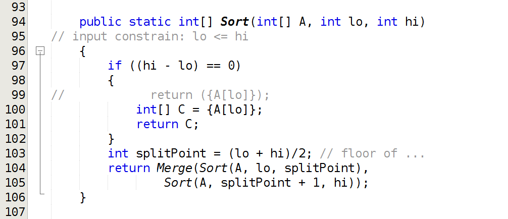
Appendix A A Java code of
Figure 6 shows a Java code of .
Appendix B Generating worst-case arrays for
Figure 7 shows a self-explanatory Java code of recursive method that given a sorted array reshuffles it, in a way resembling 5353 53 Although not with ’s sluggishness; the number of moves of keys it performs is only slightly more than the minimum number (29) of comps performed by on any -element array., onto a worst-case array for .

For instance, it produced this array of integers between 1 and 500:
1, 500, 2, 3, 4, 7, 5, 6, 8, 15, 9, 10, 11, 14, 12, 13, 16, 31, 17, 18, 19, 22, 20, 21, 23, 30, 24, 25, 26, 29, 27, 28, 32, 62, 33, 34, 35, 38, 36, 37, 39, 46, 40, 41, 42, 45, 43, 44, 47, 61, 48, 49, 50, 53, 51, 52, 54, 60, 55, 56, 57, 59, 58, 63, 124, 64, 65, 66, 69, 67, 68, 70, 77, 71, 72, 73, 76, 74, 75, 78, 92, 79, 80, 81, 84, 82, 83, 85, 91, 86, 87, 88, 90, 89, 93, 123, 94, 95, 96, 99, 97, 98, 100, 107, 101, 102, 103, 106, 104, 105, 108, 122, 109, 110, 111, 114, 112, 113, 115, 121, 116, 117, 118, 120, 119, 125, 249, 126, 127, 128, 131, 129, 130, 132, 139, 133, 134, 135, 138, 136, 137, 140, 155, 141, 142, 143, 146, 144, 145, 147, 154, 148, 149, 150, 153, 151, 152, 156, 186, 157, 158, 159, 162, 160, 161, 163, 170, 164, 165, 166, 169, 167, 168, 171, 185, 172, 173, 174, 177, 175, 176, 178, 184, 179, 180, 181, 183, 182, 187, 248, 188, 189, 190, 193, 191, 192, 194, 201, 195, 196, 197, 200, 198, 199, 202, 216, 203, 204, 205, 208, 206, 207, 209, 215, 210, 211, 212, 214, 213, 217, 247, 218, 219, 220, 223, 221, 222, 224, 231, 225, 226, 227, 230, 228, 229, 232, 246, 233, 234, 235, 238, 236, 237, 239, 245, 240, 241, 242, 244, 243, 250, 499, 251, 252, 253, 256, 254, 255, 257, 264, 258, 259, 260, 263, 261, 262, 265, 280, 266, 267, 268, 271, 269, 270, 272, 279, 273, 274, 275, 278, 276, 277, 281, 311, 282, 283, 284, 287, 285, 286, 288, 295, 289, 290, 291, 294, 292, 293, 296, 310, 297, 298, 299, 302, 300, 301, 303, 309, 304, 305, 306, 308, 307, 312, 373, 313, 314, 315, 318, 316, 317, 319, 326, 320, 321, 322, 325, 323, 324, 327, 341, 328, 329, 330, 333, 331, 332, 334, 340, 335, 336, 337, 339, 338, 342, 372, 343, 344, 345, 348, 346, 347, 349, 356, 350, 351, 352, 355, 353, 354, 357, 371, 358, 359, 360, 363, 361, 362, 364, 370, 365, 366, 367, 369, 368, 374, 498, 375, 376, 377, 380, 378, 379, 381, 388, 382, 383, 384, 387, 385, 386, 389, 404, 390, 391, 392, 395, 393, 394, 396, 403, 397, 398, 399, 402, 400, 401, 405, 435, 406, 407, 408, 411, 409, 410, 412, 419, 413, 414, 415, 418, 416, 417, 420, 434, 421, 422, 423, 426, 424, 425, 427, 433, 428, 429, 430, 432, 431, 436, 497, 437, 438, 439, 442, 440, 441, 443, 450, 444, 445, 446, 449, 447, 448, 451, 465, 452, 453, 454, 457, 455, 456, 458, 464, 459, 460, 461, 463, 462, 466, 496, 467, 468, 469, 472, 470, 471, 473, 480, 474, 475, 476, 479, 477, 478, 481, 495, 482, 483, 484, 487, 485, 486, 488, 494, 489, 490, 491, 493, 492.
It took my 3,989 comps to sort it. Of course,
Appendix C Notes from my Analysis of Algorithms lecture
Below are some of the class digital notes I wrote while lecturing Analysis of Algorithms in Spring 2012, with some comments added after class. Figure 4.14 (decision tree) is from the course textbook [2], page 177, showing a decision tree for . Note: This figure is copyrighted by Addison Wesley Longman (2000). I used it transformatively in my class for nonprofit education, criticism, and comment purposes only, and not for any other purpose, as prescribed by U.S. Code Tittle 17 Chapter 1 para 107 that established the “fair use” exception of copyrighted material.
![[Uncaptioned image]](1702.08443v1/Slide1.png)
![[Uncaptioned image]](1702.08443v1/Slide2.png)
![[Uncaptioned image]](1702.08443v1/Slide3.png)
![[Uncaptioned image]](1702.08443v1/Slide4.png)
Below is the improved recursion tree (of the Figure 4.14 page page 177 of [2]) that I used in class in Spring 2012.
![[Uncaptioned image]](1702.08443v1/RecursionTreeFixed.jpg)
References
- [1] S. Baase, Computer Algorithms: Introduction to Design and Analysis, Addison-Wesley Publishing, 2nd ed., 1991.
- [2] S. Baase and A. V. Gelder, Computer Algorithms; Introduction to Design & Analysis, Asddison Wesley, 3rd ed., 2000.
- [3] D. E. Knuth, The Art of Computer Programming, vol. 3, Addison-Wesley Publishing, 2nd ed., 1997.
- [4] R. Sedgewick and P. Flajolet, An Introduction to the Analysis of Algorithms, Pearson, 2013.
- [5] H. Steinhaus, Mathematical Snapshots, Oxford University Press, 1950.
- [6] P. K. Stockmeyer and F. F. Yao, On the optimality of linear merge, SIAM Journal on Computing, 9 (1980), p. 85–90.
- [7]
M. A. Suchenek, A complete worst-case analysis of heapsort with
experimental verifcation of its results (MS),
http://arxiv.org/abs/1504.01459, (2015). - [8]
, Best-case analysis
of MergeSort with an application to the sum of digits problem (MS),
http://arxiv.org/abs/1607.04604, (2016). - [9]
, Elementary yet
precise worst-case analysis of MergeSort (MS),
http://csc.csudh.edu/suchenek/Papers/Analysis_of_MergeSort.pdf, (2017).
©2017 Marek A. Suchenek. All rights reserved by the author.
A non-exclusive license to distribute this article is granted to arXiv.org.