Dropping Convexity for More Efficient and Scalable Online Multiview Learning
Abstract
Multiview representation learning is very popular for latent factor analysis. It naturally arises in many data analysis, machine learning, and information retrieval applications to model dependent structures among multiple data sources. For computational convenience, existing approaches usually formulate the multiview representation learning as convex optimization problems, where global optima can be obtained by certain algorithms in polynomial time. However, many evidences have corroborated that heuristic nonconvex approaches also have good empirical computational performance and convergence to the global optima, although there is a lack of theoretical justification. Such a gap between theory and practice motivates us to study a nonconvex formulation for multiview representation learning, which can be efficiently solved by a simple stochastic gradient descent (SGD) algorithm. Theoretically, we first illustrate the geometry of the nonconvex formulation; Then by characterizing the dynamics of the algorithm based on diffusion processes, we establish global rates of convergence to the global optima. Numerical experiments are provided to support our theory.
1 Introduction
Multiview data have become increasingly available in many popular real-world data analysis and machine learning problems. These data are collected from diverse domains or different feature extractors, which share latent factors. Existing literature has demonstrated different scenarios. For instance, the pixels and captions of images can be considered as two-view data, since they are two different features describing the same contents. More motivating examples involving two or more data sets simultaneously can be found in computer vision, natural language processing, and acoustic recognition. See Hardoon et al. (2004); Socher and Fei-Fei (2010); Kidron et al. (2005); Chaudhuri et al. (2009); Arora and Livescu (2012); Bharadwaj et al. (2012); Vinokourov et al. (2002); Dhillon et al. (2011). Although these data are usually unlabeled, there exist underlying association and dependency between different views, which allows us to learn useful representations in a unsupervised manner. Here we are interested in finding a representation that reveals intrinsic low-dimensional structures and decomposes underlying confounding factors. One ubiquitous approach is partial least square (PLS) for multiview representation learning. Specifically, given a data set of samples of two sets of random variables (views), and , PLS aims to find an -dimensional subspace () that preserves most of the covariance between two views. Existing literature has shown that such a subspace is spanned by the leading components of the singular value decomposition (SVD) of Arora et al. (2012), where we sample from some unknown distribution . Throughout the rest of the paper, if not clear specified, we denote by for notational simplicity.
A straightforward approach for PLS is “Sample Average Approximation” (SAA, Abdi (2003); Ando and Zhang (2005)), where we run an offline (batch) SVD algorithm on the empirical covariance matrix after seeing sufficient data samples. However, in the “big data” regime, this approach requires unfeasible amount of storage and computation time. Therefore, it is much more practical to consider the multiview learning problem in a “data laden” setting, where we draw independent samples from an underlying distribution over , one at a time. This further enables us to formulate PLS as a stochastic (online) optimization problem. Here we only consider the rank- case () for simplicity, and solve
| (1.1) |
We will explain more details on the rank- case in the later section.
Several nonconvex stochastic approximation (SA) algorithms have been proposed in Arora et al. (2012). These algorithms work great in practice, but lack theoretic justifications, since the nonconvex nature of (1.1) makes the theoretical analysis very challenging. To overcome this obstacle, Arora et al. (2016) propose a convex relaxation of (1.1). Specifically, by a reparametrization (Recall that we are interested in the rank-1 PLS), they rewrite (1.1) as11 1 For case, we replace with
| (1.2) |
where , and and are the spectral (i.e., the largest singular value of ) and nuclear (i.e., the sum of all singular values of ) norms of respectively. By examining the KKT conditions of (1.2), one can verify that is the optimal solution, where are the leading left and right singular vectors of , i.e., a pair of global optimal solutions to (1.1) for . Accordingly, they propose a projected stochastic gradient-type algorithm to solve (1.2), which is often referred to the Matrix Stochastic Gradient (MSG) algorithm. Particularly, at the -th iteration, MSG takes
where and are independently sampled from , and is a projection operator to the feasible set of (1.2). They further prove that given a pre-specified accuracy , MSG requires iterations such that with high probability.
Despite of the attractive theoretic guarantee, MSG does not present superior performance to other heuristic nonconvex stochastic optimization algorithms for solving (1.1). Although there is a lack of theoretical justification, many evidences have corroborated that heuristic nonconvex approaches not only converge to the global optima in practice, but also enjoy better empirical computational performance than the convex approaches (Zhao et al., 2015; Candes et al., 2015; Ge et al., 2015; Cai et al., 2016). Another drawback of MSG is the complicated projection step at each iteration. Although Arora et al. (2016) further propose an algorithm to compute the projection with a computational cost cubically depending on the rank of the iterates (the worst case: ), such a sophisticated implementation significantly decreases the practicability of MSG. Furthermore, MSG is also unfavored in a memory-restricted scenario, since storing the update requires real number storage. In contrast, the heuristic algorithms analyzed in this paper require only real number storage, or in the rank- case.
We aims to bridge the gap between theory and practice for solving multiview representation learning problems by nonconvex approaches. Specifically, we first illustrate the nonoconvex geometry of (1.1), we analyze the convergence properties of a simple stochastic optimization algorithm for solving (1.1) based on diffusion processes. Our analysis takes advantage of the strong Markov properties of the stochastic optimization algorithm updates and casts the trajectories of the algorithms as a diffusion processes (Ethier and Kurtz, 2009; Li et al., 2016b). By leveraging the weak convergence from discrete Markov chains to their continuous time limits, we demonstrate that the trajectories are essentially the solutions to stochastic differential equations. Such an SDE-type analysis automatically incorporates the geometry of the objective and the randomness of the algorithm, and eventually demonstrates three phases of convergence.
- 1.
Starting from an unstable equilibrium with negative curvature, the dynamics of the algorithm can be described by an Ornstein-Uhlenbeck process with a steady driven force pointing away from the initial.
- 2.
When the algorithm is sufficiently distant from the initial unstable equilibrium, the dynamics can be characterized by a deterministic ordinary differential equation (ODE). The trajectory of this phase is evolving directly toward the desired global maximum until it reaches a small basin around the global maximum.
- 3.
In this phase, the trajectory can be also described by an Ornstein-Uhlenbeck process oscillating around the global maximum. The process has a drifting term that gradually dies out and eventually becomes a nearly unbiased random walk centered at the maximum.
The sharp characterization in these three phases eventually allows us to establish strong convergence guarantees. Particularly, we show that the nonconvex stochastic gradient algorithm guarantees an -optimal solution in iterations with high probability, which is a significant improvement over convex MSG by a factor of . Our theoretical analysis reveals the power of the nonconvex optimization in PLS. The simple heuristic algorithms drop the convexity, but achieve much better efficiency.
Our convergence analysis also has important implications on stochastic optimization algorithm for Canonical Correlation Analysis (CCA). Specifically, CCA considers a similar setting to PLS, and solves
| (1.3) |
From an optimization perspective, CCA is equivalent to PLS under some linear transformation, but more challenging. We will explain more details on CCA in our later discussions.
Notations: Given a vector , we define vector norms: , , and . Given a matrix , we use to denote the -th column of and define the matrix norms and as the largest singular value of .
2 Stochastic Nonconvex Optimization
Recall that we solve (1.1)
| (2.1) |
where follows some unknown distribution . Due to the symmetrical structure of (2.1), is also a pair of global optimum. Our analysis holds for both optima. Throughout the rest of the paper, if not clearly specified, we consider as the global optimum for simplicity.
We apply the stochastic approximation (SA) of the generalized Hebbian algorithm (GHA) to solve (2.1). GHA, which is also referred as Sanger’s rule (Sanger, 1989), is essentially a primal-dual algorithm. Specifically, we consider the Lagrangian function of (2.1):
| (2.2) |
where and are Lagrangian multipliers. We then check the optimal KKT conditions,
| (2.3) |
which further imply
Solving the above equations, we obtain the optimal Lagrangian multipliers as
| (2.4) |
GHA is inspired by (2.3) and (2.4). At -th iteration GHA takes
| (2.5) |
| (2.6) |
where is the step size. Combining (2.5) and (2.6), we obtain a dual-free update as follow:
| (2.7) |
Different from the projected SGD algorithm, which is a primal algorithm proposed in Chen et al. (2017), Stochastic GHA does not need projection at each iteration.
3 Optimization Landscape
We illustrate the nonconvex optimization landscape of (1.1), which helps us understand the intuition behind the algorithmic convergence. We first study its stationary points based the Lagrangian function (2.2). By the KKT conditions (2.3), we define the stationary point of (2.2) as follows.
We then obtain all stationary points by solving (2.3). For notational simplicity, we denote . Before we proceed with our analysis, we introduce the following assumption.
Assumption 3.2.
Suppose and rank. We have , where ’s are the -th singular values of .
We impose such an eigengap assumption () to ensure the identifiability of the leading pair of singular vectors. Thus, the leading pair of singular vectors are uniquely determined only up to sign change. Let and be any pair of left and right singular matrices22 2 Since all singular values are not necessarily distinct, some pairs of singular vectors are not unique, e.g., when , and are uniquely determined up to rotation. Note that our analysis works for all possible combinations of and . See more details in Golub and Van Loan (2012).. Let and denote the -th column of and -th column of , respectively. The next proposition reveals the connection between stationary points and singular vectors.
Proposition 3.3.
The proof of Proposition 3.3 is presented in Appendix A.1. We then determine the types of these obtained stationary points. The next proposition characterizes the maximum eigenvalues of at these stationary points of (2.2).
Proposition 3.4.
4 Global Convergence by ODE
Before we proceed with our analysis, we first impose some mild assumptions on the problem.
Assumption 4.1.
are data samples identically independently distributed as respectively satisfying the following conditions:
- 1.
For any , and for a constant ;33 3 We only need ()-th moments of and to be bounded, while the preliminary results in Chen et al. (2017) require both and to be bounded random variables.
- 2.
, where ’s are the singular values of .
Here we assume and are of the same dimensions (i.e., ) and is full rank for convenience of analysis. The extension to in a rank deficient setting is straightforward, but more involved (See more details in Section 5.4). Moreover, for a multiview learning problem, it is also natural to impose the following additional assumptions.
Assumption 4.2.
Given the observed random variables and , there exist two orthogonal matrices such that , where and are the latent variables satisfying:
- 1.
and are uncorrelated if , so that and are the left and right singular matrices of respectively;
- 2.
, where , and are constants.
The next proposition characterizes the strong Markov property of our algorithm.
Proposition 4.3.
Using (2.7), we get a sequence of . They form a discrete-time Markov process.
With Proposition 4.3, we can construct a continuous time process to derive an ordinary differential equation to analyze the algorithmic convergence. Specifically, as the fixed step size , two processes based on the sequence generated by (2.7), weakly converge to the solution of the following ODE system in probability (see more details in Ethier and Kurtz (2009)),
| (4.1) |
where and . To highlight the sequence generated by (2.7) depending on , we redefine .
Theorem 4.4.
As , the processes weakly converge to the solution of the ODE system in (4.1) with sphere initial , i.e., .
The proof of Theorem 4.4 is presented in Appendix B.1. Under Assumption 4.1, the above ODE system admits a closed form solution. Specifically, we solve and simultaneously, since they are coupled together in (4.1). To simplify (4.1), we define and . We then rewrite (4.1)as
| (4.2) |
where . By Assumption 4.2, and are the left and right singular matrices of respectively, i.e., , where is diagonal. For notational simplicity, we define such that . One can verify , where
By left multiplying both sides of (4.2), we obtain
| (4.7) |
which is a coordinate separable ODE system. Accordingly, we define ’s as:
| (4.8) |
Thus, we can obtain a closed form solution to (4.7) based on the following theorem.
Theorem 4.5.
Given (4.7), we write the ODE in each component ,
| (4.9) |
where when . This ODE System has a closed form solution as follows:
| (4.10) |
for , where
is a normalization function such that .
The proof of Theorem 4.5 is presented in Appendix B.2. Without loss of generality, we assume . As can be seen, , as . We have successfully characterized the global convergence performance of our algorithm with an approximate error . The solution to the ODE system in (4.10), however, does not fully reveal the algorithmic behavior (more precisely, the rate of convergence) near the equilibria of the ODE system. This further motivates us to exploit the stochastic differential equation approach to characterize the dynamics of the algorithm.
5 Global Dynamics by SDE
We analyze the dynamics of the algorithm near the equilibria based on stochastic differential equation by rescaling analysis. Specifically, we characterize three stages for the trajectories of solutions: [a] Neighborhood around unstable equilibria — minimizers and saddle points of (2.1), [b] Neighborhood around stable equilibria — maximizers of (2.1), and [c] deterministic traverses between equilibria. Moreover, we provide the approximate the number of iterations in each phase until convergence.
5.1 Phase I: Escaping from Unstable Equilibria
Suppose that the algorithm starts to iterate around a unstable equilibrium, (e.g. saddle point). Different from our previous analysis, we rescale two aforementioned processes and rescaled by a factor of . This eventually allows us to capture the uncertainty of the algorithm updates by stochastic differential equations. Roughly speaking, the ODE approximation is essentially a variant of law of large number for Markov process, while the SDE approximation serves as a variant of central limit theorem accordingly.
Recall that is an orthonormal matrix for diagonalizing Q, and is defined in (4.7). Let and denote the -th coordinates of and respectively. The following theorem characterizes the dynamics of the algorithm around the unstable equilibrium.
Theorem 5.1.
Suppose is initialized around some saddle point or minimizer (e.g. -th column of with ), i.e., and for . Then for any there exist and such that
| (5.1) |
Proof Sketch.
We prove this argument by contradiction. Assume the conclusion does not hold, that is there exists a constant such that for any we have
That implies there exists a sequence converging to such that
| (5.2) |
Then we show is tight and thus converges weakly. Furthermore, weakly converges to a stochastic differential equation,
| (5.3) |
We compute the solution of this stochastic differential equation and then show (5.1) does not hold. ∎
Theorem 5.1 implies that for , with a constant probability , escapes from the saddle points at some time , i.e., is smaller than , where . Note that (5.3) is a Fokker-Planck equation, which admits a closed form solution as follows,
| (5.4) |
Such a solution is well known as the Ornstein-Uhlenbeck process (Øksendal, 2003), and also implies that the distribution of can be well approximated by the normal distribution of for a sufficiently small step size. This continuous approximation further has the following implications:
- [a]
For is essentially a random variable with mean and variance smaller than . The larger is, the closer its variance gets to this upper bound. While essentially amplifies by a factor exponentially increasing in . This tremendous amplification forces to quickly get away from , as increases.
- [b]
For , we have
As has been shown in [a] that does not need to be large for to get away from . Here we only consider relatively small . Since the initial drift for is very small, tends to stay at . As increases, the exponential decay term makes the drift quickly become negligible. Moreover, by mean value theorem, we know that the variance is bounded, and increases far slower than the variance in [a]. Thus, roughly speaking, oscillates near .
- [c]
For , we have and . This implies that also tends to oscillate around , as increases.
Overall speaking, [a] is dominative so that it is the major driving force for the algorithm to escape from this unstable equilibrium. More precisely, let us consider one special case for Phase I, that is we start from the second maximum singular value, with . We then approximately calculate the number of iterations to escape Phase I using the algorithmic behavior of with by the following proposition.
Proposition 5.2.
Given pre-specified and sufficiently small , there exists some , where is a generic constant, such that the following result holds: We need at most
iterations such that with probability at least , where is the CDF of standard normal distribution.
5.2 Phase II: Traverse between Equilibria
When the algorithm is close to neither the saddle points nor the optima, the algorithm’s performance is nearly deterministic. Since is a rescaled version of , their trajectories are similar. Like before, we have the following proposition to calculate the approximate iterations, , following our results in Section 4. We restart the counter of iteration by Proposition 4.3.
Proposition 5.3.
After restarting counter of iteration, given sufficiently small and defined in Proposition 5.2, we need at most
iterations such that .
5.3 Phase III: Convergence to Stable Equilibria
Again, we restart the counter of iteration by the strong Markov property. The trajectory and analysis are similar to Phase I, since we also characterize the convergence using an Ornstein-Uhlenbeck process. The following theorem characterizes the dynamics of the algorithm around the stable equilibrium.
Theorem 5.4.
Suppose is initialized around some maximizer (the first column of ), i.e., and for . Then as , for all , weakly converges to a diffusion process satisfying the following SDE for ,
| (5.5) |
where is a brownian motion, and
The proof of Theorem 5.4 is provided in Appendix C.4. Similar to (5.4), the closed form solution to (5.5) for is as follow:
| (5.6) |
By the property of the O-U process, we characterize the expectation and variance of for .
Recall that the distribution of can be well approximated by the normal distribution of for a sufficiently small step size. This further implies that after sufficiently many iterations, SGD enforces except . Meanwhile, SGD behaves like a biased random walk towards the optimum, when it iterates within a small neighborhood the optimum. But unlike Phase I, the variance gradually becomes a constant.
Based on theorem 5.4, we further establish an iteration complexity bound for SGD in following proposition.
Proposition 5.5.
Given a pre-specified , a sufficiently small , and defined in Proposition 5.2, after restarting counter of iteration, we need at most
iterations such that with probability at least .
The proof of Proposition 5.5 is provided in Appendix C.5. Combining Propositions 5.2, 5.3, and 5.5, we obtain a more refined result in the following corollary.
Corollary 5.6.
Given a sufficiently small pre-specified , we choose
We need at most
iterations such that we have with probability at least
The proof of Corollary 5.6 is provided in Appendix C.6. We can further improve the probability to for some by repeating replicates of SGD. We then compute the geometric median of all output solutions. See more details in Cohen et al. (2016).
5.4 Extension to
Our analysis can further extend to the case where and have different dimensions, i.e., . Specifically, we consider an alternative way to construct defined in (4). We follow the same notations to Assumption 4.2, and use and to denote the transition matrix between the observed data and latent variables. The dimensions of and , however, are different now, i.e., and . Without loss of generality, we assume and , where and , and are the transform matrix of and , respectively. Then we have the singular value decomposition as follows,
Thus, we have and . Now we design the orthogonal transform matrix .
One can check that
Then our previous analysis using ODE and SDE still holds.
Note that for , any column vector of in (4) is a stationary solution. Here the square matrix in (5.4) contains column vectors, but only the first and last column vectors are stationary solutions. This is because the remaining column vectors are even not feasible solutions, and violate the constraint . Thus, given a feasible initial, the algorithm will not be trapped in the subspace spanned by th remaining column vectors .
5.5 Extension to Missing Values
Our methodology and theory can tolerate missing values. For simplicity, we assume the entries of and misses independently with probability in each iteration, where . We then set all missing entries as values. We denote such imputed vectors by and . One can verify is an unbiased estimator of . Note that can be further absorbed into the step size , denoted by . Then (2.7) becomes:
| (5.18) |
The convergence analysis is very similar to the standard setting with a different choice of , and therefore is omitted.
6 Numerical Experiments
We first provide a simple example to illustrate our theoretical analysis. Specifically, we choose . We first generate the joint covariance matrix for the latent factors and as
and . We then generate two matrices and with each entry independently sampled from . Then we convert and to orthonormal matrices and by Grand-Schmidt transformation. At last, we generate the joint covariance matrix for the observational random vectors and using the following covariance matrix
We consider the total sample size as and choose . The initialization solution is a pair of singular vectors associated with the second largest singular value of , i.e., saddle point. We repeat the simulation with update (2.7) for times, and plot the obtained results.
Figure 1(a) illustrates the three phases of the SGD algorithm. Specifically, the horizontal axis is the number of iterations, and the vertical axis is defined in (4.8). As , we have and , e.g., global optima. This is due to the symmetric structure of the problem as mentioned in Section 1. Figure 1(a) is consistent with our theory: In Phase I, the algorithm gradually escapes from the saddle point; In Phase II, the algorithm quickly moves towards the optimum; In Phase III, the algorithm gradually converges to the optimum.
Figure 1(b) further zooms in Phase I of Figure 1(a). We see that the trajectories of all simulations behave very similar to an O-U process. Figure 1(c) illustrates the three phases by . As our analysis suggests, when , we have . We see that the trajectories of all simulations also behave very similar to an O-U process in Phase III. These experimental results are consistent with our theory.


Also, we illustrate in Phase I and in Phase III are O-U processes by showing that 100 simulations of follow gaussian distributions at -th, -th, and -th iteration and those of follow gaussian distributions at -th, -th, and -th iteration. This is consistent with the Theorems 5.1 and 5.4 in Section 5. Also as we can see that in the Phase I, the variance of becomes larger and larger when the iteration number increases. Similarly, in the Phase III, the variance of becomes closer to a fixed number.


We then provide a real data experiment for comparing the computational performance our nonconvex stochastic gradient algorithm for solving (2.1) with the convex stochastic gradient algorithm for solving (1.2). We choose a subset of the MNIST dataset, whose labels are . The total sample size is , and . As Arora et al. (2016) suggest, we choose or , for the convex stochastic gradient algorithm. For our nonconvex stochastic gradient algorithm, we choose either , , or . Figure 3 illustrates the computational performance in terms of iterations and wall clock time. As can be seen, our nonconvex stochastic gradient algorithm outperforms the convex counterpart in iteration complexity, and significantly outperforms in wall clock time, since the nonconvex algorithm does not need the computationally expensive projection in each iteration. This suggests that dropping convexity for PLS can boost both computational scalability and efficiency.


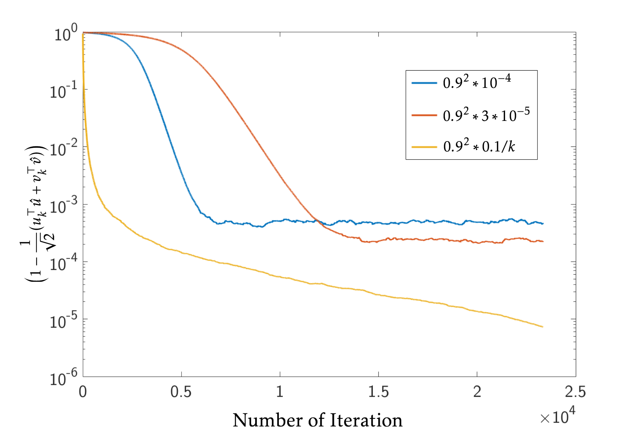
Our last experiment demonstrates the computational performance of our proposed SGD algorithm when there exist missing values. Specifically, we adopt the same MNIST data set as our previous experiment. We independently drop each pixel of the image in each iteration with probability . Figure 4 illustrates the computational performance in terms of iterations under different missing probability and choices of the step size parameter. As can be seen, the empirical convergence of our proposed SGD algorithm is similar to (but slower than) that of our previous experiment without missing values.
7 Discussions
We establish the convergence rate of stochastic gradient descent (SGD) algorithms for solving online partial least square (PLS) problems based on diffusion process approximation. Our analysis indicates that for PLS, dropping convexity actually improves efficiency and scalability. Our convergence results are tighter than existing convex relaxation based method by a factor of , where is a pre-specified error. We believe the following directions should be of wide interests:
- 1.
Our current results hold only for the top pair of left and right singular vectors, i.e., . For , we need to solve
(7.1) Our approximations using ODE and SDE, however, do not admit unique solution due to rotation or permutation. Thus, extension of our analysis to is a challenging, but also an important future direction.
- 2.
Our current results are only applicable to a fixed step size . Our experiments suggest that the diminishing step size , from 1 to , where is the sample complexity from theory, achieves a better empirical performance. One possible probability tool is Stein’s method (Ross et al., 2011).
- 3.
Our current results rely on the classical central limit theorem-type analysis by taking . Note the analysis of is an asymptotic result, and in experiment, when is small, and exactly stay on the sphere. But to get a more general result, connecting our analysis to discrete algorithmic proofs such as Jain et al. (2016); Shamir (2015); Li et al. (2016a) should be an important direction (Barbour and Chen, 2005). One possible probability tool for addressing this issue is Stein’s method (Ross et al., 2011).
Moreover, our proposed SGD algorithm for PLS is also closely related to Canonical Correlation Analysis. Specifically, CCA solves a similar problem
| (7.2) |
For notational simplicity, we denote , , and . Since computing and is not affordable, the projected stochastic gradient algorithms are not applicable. Thus we consider an alternative approach to avoid the projection operation. We consider the Lagrangian function of (7.2) as
| (7.3) |
where and are Lagrangian multipliers. We then check the optimal KKT conditions,
which further imply
Solving the above equations, we obtain the optimal Lagrangian multipliers as
| (7.4) |
Similarly, we then apply the dual free stochastic gradient method to solve (7.2). Specifically, at the -th iteration, we independently sample and from . Then we obtain
| (7.5) |
Here we sample two pairs of and to ensure the unbiasedness of the stochastic gradient.
Then we can convert (7.5) to ordinary differential equations by taking , we get
Different from PLS, the above ordinary differential equations do not admit a closed form solution, which makes our ODE/SDE-type convergence analysis not applicable in a straightforward manner. A possible alternative approach is to establish the lower bounds for and , and further prove that as , we have and . We will leave this option for further investigation.
Taking our result for PLS as an initial start, we expect more sophisticated and stronger follow-up work that applies to CCA and other online optimization problems with similar structures, which eventually benefits the learning community in both practice and theory.
References
- Abdi (2003) Abdi, H. (2003). Partial least square regression (pls regression). Encyclopedia for research methods for the social sciences 792–795.
- Ando and Zhang (2005) Ando, R. K. and Zhang, T. (2005). A framework for learning predictive structures from multiple tasks and unlabeled data. Journal of Machine Learning Research 6 1817–1853.
- Arora et al. (2012) Arora, R., Cotter, A., Livescu, K. and Srebro, N. (2012). Stochastic optimization for pca and pls. In Communication, Control, and Computing (Allerton), 2012 50th Annual Allerton Conference on. IEEE.
- Arora and Livescu (2012) Arora, R. and Livescu, K. (2012). Kernel cca for multi-view learning of acoustic features using articulatory measurements. In MLSLP. Citeseer.
- Arora et al. (2016) Arora, R., Mianjy, P. and Marinov, T. (2016). Stochastic optimization for multiview representation learning using partial least squares. In Proceedings of The 33rd International Conference on Machine Learning.
- Barbour and Chen (2005) Barbour, A. D. and Chen, L. H. Y. (2005). An introduction to Stein’s method, vol. 4. World Scientific.
- Bharadwaj et al. (2012) Bharadwaj, S., Arora, R., Livescu, K. and Hasegawa-Johnson, M. (2012). Multiview acoustic feature learning using articulatory measurements. In Intl. Workshop on Stat. Machine Learning for Speech Recognition. Citeseer.
- Cai et al. (2016) Cai, T. T., Li, X., Ma, Z. et al. (2016). Optimal rates of convergence for noisy sparse phase retrieval via thresholded wirtinger flow. The Annals of Statistics 44 2221–2251.
- Candes et al. (2015) Candes, E. J., Li, X. and Soltanolkotabi, M. (2015). Phase retrieval via wirtinger flow: Theory and algorithms. IEEE Transactions on Information Theory 61 1985–2007.
- Chaudhuri et al. (2009) Chaudhuri, K., Kakade, S. M., Livescu, K. and Sridharan, K. (2009). Multi-view clustering via canonical correlation analysis. In Proceedings of the 26th annual international conference on machine learning. ACM.
- Chen et al. (2017) Chen, Z., Yang, L. F., Li, C. J. and Zhao, T. (2017). Online partial least square optimization: Dropping convexity for better efficiency and scalability. In Proceedings of The 34th International Conference on Machine Learning.
- Cohen et al. (2016) Cohen, M. B., Lee, Y. T., Miller, G., Pachocki, J. and Sidford, A. (2016). Geometric median in nearly linear time. In Proceedings of the 48th Annual ACM SIGACT Symposium on Theory of Computing. ACM.
- Dhillon et al. (2011) Dhillon, P., Foster, D. P. and Ungar, L. H. (2011). Multi-view learning of word embeddings via cca. In Advances in Neural Information Processing Systems 24 (J. Shawe-Taylor, R. S. Zemel, P. L. Bartlett, F. Pereira and K. Q. Weinberger, eds.). Curran Associates, Inc., 199–207.
- Ethier and Kurtz (2009) Ethier, S. N. and Kurtz, T. G. (2009). Markov processes: characterization and convergence, vol. 282. John Wiley & Sons.
- Evans (1988) Evans, W. (1988). Partial differential equations.
- Ge et al. (2015) Ge, R., Huang, F., Jin, C. and Yuan, Y. (2015). Escaping from saddle points-online stochastic gradient for tensor decomposition. In COLT.
- Golub and Van Loan (2012) Golub, G. H. and Van Loan, C. F. (2012). Matrix computations, vol. 3. JHU Press.
- Hardoon et al. (2004) Hardoon, D. R., Szedmak, S. and Shawe-Taylor, J. (2004). Canonical correlation analysis: An overview with application to learning methods. Neural computation 16 2639–2664.
- Jain et al. (2016) Jain, P., Jin, C., Kakade, S. M., Netrapalli, P. and Sidford, A. (2016). Streaming pca: Matching matrix bernstein and near-optimal finite sample guarantees for oja’s algorithm. In 29th Annual Conference on Learning Theory.
- Kidron et al. (2005) Kidron, E., Schechner, Y. Y. and Elad, M. (2005). Pixels that sound. In Computer Vision and Pattern Recognition, 2005. CVPR 2005. IEEE Computer Society Conference on, vol. 1. IEEE.
- Li et al. (2016a) Li, C. J., Wang, M., Liu, H. and Zhang, T. (2016a). Near-optimal stochastic approximation for online principal component estimation. arXiv preprint arXiv:1603.05305 .
- Li et al. (2016b) Li, C. J., Wang, Z. and Liu, H. (2016b). Online ica: Understanding global dynamics of nonconvex optimization via diffusion processes. In Advances in Neural Information Processing Systems.
- Nowakowski (2013) Nowakowski, B. D. (2013). On multi-parameter semimartingales, their integrals and weak convergence .
- Øksendal (2003) Øksendal, B. (2003). Stochastic differential equations. In Stochastic differential equations. Springer, 65–84.
- Ross et al. (2011) Ross, N. et al. (2011). Fundamentals of stein’s method. Probab. Surv 8 210–293.
- Sanger (1989) Sanger, T. D. (1989). Optimal unsupervised learning in a single-layer linear feedforward neural network. Neural networks 2 459–473.
- Shamir (2015) Shamir, O. (2015). Fast stochastic algorithms for svd and pca: Convergence properties and convexity. arXiv preprint arXiv:1507.08788 .
- Socher and Fei-Fei (2010) Socher, R. and Fei-Fei, L. (2010). Connecting modalities: Semi-supervised segmentation and annotation of images using unaligned text corpora. In Computer Vision and Pattern Recognition (CVPR), 2010 IEEE Conference on. IEEE.
- Vinokourov et al. (2002) Vinokourov, A., Shawe-Taylor, J. and Cristianini, N. (2002). Inferring a semantic representation of text via cross-language correlation analysis. In NIPS, vol. 1.
- Zhao et al. (2015) Zhao, T., Wang, Z. and Liu, H. (2015). A nonconvex optimization framework for low rank matrix estimation. In Advances in Neural Information Processing Systems.
Appendix A Proof Detailed Proofs in Section 3
A.1 Proof of Proposition 3.3
Proof.
We consider a compact singular value decomposition of as follow:
where are nonzero singular values, and ’s are a pair of singular vectors associated with . Plugging (2.4) into (2.3), we have
| (A.1) |
Since every vector and can be expanded as
| (A.2) |
where for and for are orthonormal basis vectors, and complementary to ’s and ’s for in and respectively, and ’s and ’s are the coefficients. Plugging (A.2) into the first equation of (A.1), we get
| (A.3) |
The second equality holds because and are the columns of the orthogonal matrices. Since ’s are the basis vectors of , by (A.3), we know the coefficients of all ’s should be . Therefore we consider two scenarios:
- 1.
- 2.
If , then we have , , which further leads to:
(A.4) Note that (A.4) holds if and only if there exists only one where is the Kronecker delta, i.e.,
The verification of the above points satisfying (A.1) is straightforward, and therefore omitted. ∎
A.2 Proof of Proposition 3.4
Proof.
For notation simplicity, we denote as
- a.
If and are in the row and column null space of respectively, then
Therefore, it is an unstable stationary point because of the positive curvature.
- b.
If is a pair of singular vector of , then by simple linear algebra, we know that
One can verify
Therefore, the Hessian matrix is negative semi-definite if and only if , i.e., is the optimum of (1.1). The Hessian has a positive eigenvalue.
Thus, only the optima of (2.2) are stable stationary points. All the others are unstable. ∎
Appendix B Proof Detailed Proofs in Section 4
B.1 Proof of Theorem 4.4
Proof.
First, we calculate the infinitesimal conditional expectation. Since the optimization problem is symmetric about and , we only prove the claim for ,
Next, we show that if the initial is on the sphere, then with probability , all iterations are on the sphere as . Given , we have
Therefore, we get
The last equality holds, since is finite:
Finally, we bound the infinitesimal conditional variance.
Last equality holds by the Assumption 4.1.
Therefore, by Section 4 of Chapter 7 in Ethier and Kurtz (2009), we know that, as , and weakly converge to the solution of (4.1) with the same initial. By definition of and , we complete the proof. ∎
B.2 Proof of Theorem 4.5
Proof.
Since is an orthonormal matrix, for all . Thus, we have
We then verify (4.10) satisfies (4.9). By Evans (1988), we know that since is continuously differentiable in , the solution to the ODE is unique. For notational simplicity, we denote
Then we have
Now we only need to verify
which completes the proof. ∎
Appendix C Proof Detailed Proofs in Section 5
C.1 Proof of Theorem 5.1
Proof.
We prove this by contradiction. Assume the conclusion does not hold, that is there exists a constant such that for any we have
That implies there exists a sequence converging to such that
| (C.1) |
Thus, condition (i) in Theorem 2.4 (Nowakowski, 2013) holds. We next check the second condition. When holds, Assumption 4.1 yields that where is some constant. Thus, for any we have
Thus, condition (ii) in Theorem Theorem 2.4 (Nowakowski, 2013) holds. Then we have is tight and thus converges weakly.
We then calculate the infinitesimal conditional expectation and variance for .
| (C.2) |
where the last equality comes from the assumption that the algorithm starts near column of , i.e., . To compute variance, we first compute ,
where is defined in (4.2). Then we analyze by cases:
which further implies
| (C.3) |
By (C.2) and (C.3), we get the limit stochastic differential equation,
Therefore, converges weakly to a solution of The process defined by the equation above is an unstable O-U process with mean and exploding variance. Thus, for any , there exist a time , such that
Since converges weakly to thus converges in distribution to This implies that there exists an , such that for any
Then we find a such that
or equivalently
Since we have
which leads to a contradiction with C.1. Our assumption does not hold.
∎
C.2 Proof of Proposition 5.2
Proof.
Our analysis is based on approximating by its continuous approximation , which is normal distributed at time . By simple manipulation, we have
We then prove . At time t, approximates to a normal distribution with mean and variance . Therefore, let be the CDF of , we have
which requires
Solving the above inequality, we get
∎
C.3 Proof of Proposition 5.3
Proof.
After Phase I, we restart our counter, i.e., . By (4.10) and approximating to the process , we obtain
which requires
Solving the above inequality, we get
∎
C.4 Proof of Theorem 5.4
Proof.
For , we compute the infinitesimal conditional expectation and variance,
Following similar lines to the proof of Theorem 5.1, by Section 4 of Chapter 7 in Ethier and Kurtz (2009), we have for each if as , then the stochastic process weakly converges to the solution of the stochastic differential equation (5.5). ∎
C.5 Proof of Proposition 5.5
Proof.
Since we restart our counter, we have . Since approximates to and its second moment:
we use the Markov inequality:
To guarantee , we get:
∎
C.6 Proof of Corollary 5.6
Proof.
First, we prove that can be bounded by , when it is near the optima. Recall that and . Our analysis has shown that when is large enough, the SGD iterates near the optima. Then we have
| (C.4) |
where the last inequality holds since is large enough such that is sufficiently small. By Propositions 5.2, 5.3, and 5.5, the total iteration number is
| (C.5) |
To explicitily bound in (C.5) in terms of sample size n, we consider
| (C.6) | ||||
| (C.7) | ||||
| (C.8) |
Given a small enough we choose as follow:
| (C.9) |
Combining the above sample complexities (C.6), (C.7), (C.8), and (C.9), we get
| (C.10) |
By Proposition 5.5 with (C.4), after at most iterations, we have
with probability at least . ∎