Correlators in simultaneous measurement of non-commuting qubit observables

Continuous quantum measurements (CQMs) have become a unique platform to explore fundamental aspects of quantum phenomena and have potential applications to quantum information science. They have been discussed theoretically in various contexts (e.g., [1, 2, 3, 4, 5, 6, 7, 8, 9, 10]), and in the past decade superconducting qubits have become the main experimental system for the realization of CQMs [11, 12, 13, 14, 15, 16, 17]. CQMs are shedding new light on our understanding of the quantum measurement process, and there is also a growing interest in CQM applications, including quantum feedback [18, 19, 20, 13, 16], rapid state purification [21], preparation of entangled states [22, 23, 24], and continuous quantum error correction [25, 26].

While a simultaneous measurement of non-commuting observables is impossible with projective measurements, nothing theoretically forbids such a measurement using CQMs. Aside from new physics, such a protocol may open up new areas of applications, inaccessible to projective measurements. The theoretical discussion of a simultaneous measurement of incompatible observables has a long history [27, 28, 29, 30]. For the measurement of non-commuting observables of a qubit, statistics of time-integrated detector outputs and fidelity of state monitoring directly via time-integrated outputs has been analyzed in Ref. [31]. The evolution of the qubit state due to simultaneous measurement of incompatible variables has been described theoretically in Ref. [32], and has been recently demonstrated experimentally in Ref. [33].

In this letter, we focus on the temporal correlations of the output signals from two linear detectors measuring continuously and simultaneously the qubit observables $\sigma_{z}$ and $\sigma_{\varphi}\equiv\sigma_{z}\cos\varphi+\sigma_{x}\sin\varphi$, where $\sigma_{x}$ and $\sigma_{z}$ are the Pauli matrices and $\varphi$ is an angle between the two measurement directions on the Bloch sphere (Fig. 1). The experimental setup is described in detail in Ref. [33]; it is based on a Rabi-rotated physical qubit, which is measured stroboscopically [34] using symmetric sideband pumping of a coupled resonator, so that $\sigma_{z}$ and $\sigma_{\varphi}$ for an effective rotating-frame qubit are being measured. Description of such a measurement based on the theory of quantum trajectories [8, 9, 35, 36] has been developed in Ref. [33]. In this letter we will use a simpler approach based on quantum Bayesian theory [10, 37]. The quantum Bayesian description of the rotating-frame experiment [33] is developed in the Supplemental Material [38]. The goal of this letter is calculation of the time-correlators for the output signals measuring $\sigma_{z}$ and $\sigma_{\varphi}$, and their comparison with experimental data. As we will see, these correlators may be a useful tool for sensitive parameter estimation in an experiment. These correlators are also important in the analysis of quantum error detection and correction based on simultaneous measurement of non-commuting operators [39]. We note that the analyzed output signal correlators are different from qubit-state correlators [40].

Quantum Bayesian theory.—A simultaneous continuous measurement of the qubit observables $\sigma_{z}$ and $\sigma_{\varphi}$ by two linear detectors (Fig. 1) produces noisy output signals $I_{z}(t)$ and $I_{\varphi}(t)$, respectively [32, 37],

where $\rho(t)$ is the qubit density matrix and $\tau_{z}$, $\tau_{\varphi}$ are the “measurement” (collapse) times needed for an informational signal-to-noise ratio of 1 for each channel. Note the chosen normalization for $I_{z}$ and $I_{\varphi}$. In the Markovian approximation, the noises $\xi_{z}$ and $\xi_{\varphi}$ are uncorrelated, white, and Gaussian with two-time correlators

and $\langle\xi_{z}(t)\,\xi_{\varphi}(t^{\prime})\rangle=0$. The qubit state is characterized in the Bloch-sphere representation as $\rho(t)\equiv\left[\openone+x(t)\,\sigma_{x}+y(t)\,\sigma_{y}+z(t)\,\sigma_{z}\right]/2$. We assume phase-sensitive amplifiers in the experimental setup, amplifying the optimal (informational) quadratures, so that the qubit evolution due to measurement is not affected by the phase backaction related to fluctuations in the orthogonal (non-informational) quadrature [35, 36, 37]. Then there is only the quantum informational backaction, which for measurement of $\sigma_{z}$ and $\sigma_{\varphi}$ is described [32, 37, 38] by the evolution equations (in the Itô interpretation)

Here $\Gamma_{z}$ and $\Gamma_{\varphi}$ are the ensemble dephasing rates due to measurement, so that the quantum efficiencies [37] for the two channels are $\eta_{z}=1/(2\tau_{z}\Gamma_{z})$ and $\eta_{\varphi}=1/(2\tau_{\varphi}\Gamma_{\varphi})$. In the experiment $\eta_{z}=0.49$ and $\eta_{\varphi}=0.41$.

Equations (4)–(6) describe qubit evolution only due to measurement. We also need to add terms due to unitary evolution and due to decoherence not related to measurement. We assume the Hamiltonian $H=\hbar\tilde{\Omega}_{\rm R}\sigma_{y}/2$, describing Rabi oscillations about $y$-axis with frequency $\tilde{\Omega}_{\rm R}$. In the experiment, $\tilde{\Omega}_{\rm R}=\Omega_{\rm R}-\Omega_{\rm rf}$ is a small (kHz-range) undesired mismatch between the physical qubit Rabi frequency $\Omega_{\rm R}$ and rotating frame frequency $\Omega_{\rm rf}$ defined by detuning of sideband pumps [33, 38]. Decoherence of the effective qubit arises from the decoherence of the physical qubit with energy relaxation time $T_{1}$ and dephasing time $T_{2}$ [the pure dephasing rate is then $T_{\rm pd}^{-1}=T_{2}^{-1}-(2T_{1})^{-1}$]. Averaging the decoherence over fast rotation $\Omega_{\rm R}\gg T_{2}^{-1}$ and adding unitary evolution, we obtain [38]

Evolution of the effective qubit is described by adding terms from Eqs. (4)–(6) and (7).

Correlators.—Our next goal is to calculate the two-time correlators, $K_{ij}(\tau)$, for the output signals,

Self- and cross-correlators correspond to $i=j$ and $i\neq j$, respectively. The averaging in Eq. (9) is over an ensemble of measurements with the initial qubit state $\rho_{\rm in}$ prepared at time $t_{\rm in}\leq t_{1}$. We will see, however, that the result does not depend on $\rho_{\rm in}$, $t_{\rm in}$, and $t_{1}$, so Eq. (9) can also be understood as averaging over time $t_{1}$. We assume that the parameters in Eqs. (4)–(7) do not change with time. By assuming $\tau>0$, we avoid considering the trivial zero-time contribution to the self-correlators, $\Delta K_{ii}(\tau)=\tau_{i}\,\delta(\tau)$.

As shown in the Supplemental Material [38], calculation of the correlators from Eqs. (1)–(7) is equivalent to the following recipe [41]: we replace an actual continuous measurement at the (earlier) time moment $t_{1}$ with a projective measurement of $\sigma_{i}$, so that the measurement result $I_{i}(t_{1})$ is $\pm 1$ with probability $\{1\pm{\rm Tr}[\sigma_{i}\,\rho(t_{1})]\}/2$, and the qubit state collapses correspondingly to the eigenstate $|1_{i}\rangle$ or $|0_{i}\rangle$ of $\sigma_{i}$ ($\sigma_{i}|1_{i}\rangle=|1_{i}\rangle$, $\sigma_{i}|0_{i}\rangle=-|0_{i}\rangle$). This gives the correlator

where $\rho_{\rm av}(t_{1}+\tau|1_{i})$ is the ensemble-averaged density matrix at time $t_{1}+\tau$ with the initial condition $\rho_{\rm av}(t_{1}|1_{i})=|1_{i}\rangle\langle 1_{i}|$; similarly, $\rho_{\rm av}(t_{1}+\tau|0_{i})$ starts with $\rho_{\rm av}(t_{1}|0_{i})=|0_{i}\rangle\langle 0_{i}|$. The evolution of $\rho_{\rm av}$ is given by Eqs. (4)–(7) without noise, $\xi_{z}=\xi_{\varphi}=0$ (because of the Itô form), so that

These equations have an analytical solution presented in [38] (note that the evolution of the $y$-coordinate is not important in our analysis). Thus we obtain the following correlators (alternative methods for the derivation are also discussed in [38]):

Because of the rotational symmetry, the results for the correlators $K_{\varphi\varphi}(\tau)$ and $K_{\varphi z}(\tau)$ can be obtained from Eqs. (14) and (15) by exchanging $\Gamma_{z}\leftrightarrow\Gamma_{\varphi}$ and $\varphi\to-\varphi$. The rotational symmetry also makes the correlators insensitive to a $y$-rotation in both measurement directions, $z\rightarrow\varphi_{\rm add}$, $\varphi\rightarrow\varphi+\varphi_{\rm add}$, by any angle $\varphi_{\rm add}$.

We emphasize that the obtained correlators do not depend on the qubit state $\rho(t_{1})$ and therefore on $\rho_{\rm in}$ and $t_{\rm in}$ (this property would not hold in the presence of phase backaction). We also emphasize that the correlators depend on $\Gamma_{z}$ and $\Gamma_{\varphi}$, but do not depend on $\tau_{z}$ and $\tau_{\varphi}$ and therefore on the quantum efficiencies $\eta_{z}$ and $\eta_{\varphi}$. Physically, this is because non-ideal detectors can be thought of as ideal detectors with extra noise at the output [37], which only affects the zero-time self-correlators $K_{ii}(0)$.

Let us discuss some special cases for the results (14)–(16). (i) At small times, $\tau\to+0$, we obtain correlators

(ii) For $|\varphi|\ll 1$ and sufficiently small $T_{2}^{-1}$ and $\tilde{\Omega}_{\rm R}$, we have Zeno pinning near the states $|0\rangle$ and $|1\rangle$ with rare jumps between them with equal rates $\Gamma_{\rm jump}$. This produces cross-correlator [42] $K_{z\varphi}(\tau)\approx\exp(-2\Gamma_{\rm jump}\tau)$ with jump rates

(iii) In the case $\tilde{\Omega}_{\rm R}=T_{1}^{-1}=T_{2}^{-1}=0$, we have full correlation for $\varphi=0$, $K_{z\varphi}(\tau)=K_{zz}(\tau)=1$, full anticorrelation for $\varphi=\pi$, $K_{z\varphi}(\tau)=-K_{zz}(\tau)=-1$, and no correlation for $\varphi=\pi/2$, $K_{z\varphi}(\tau)=0$, while $K_{zz}(\tau)=e^{-\Gamma_{\varphi}\tau}$ and $K_{\varphi\varphi}(\tau)=e^{-\Gamma_{z}\tau}$. (iv) In the case $\tilde{\Omega}_{\rm R}=0$, the cross-correlator is symmetric, $K_{z\varphi}(\tau)=K_{\varphi z}(\tau)$, for any $\varphi$.

Comparison with experimental results.—Experimental data have been taken in the same way as in Ref. [33] (see also [38]). Experimental parameters correspond to well-separated frequency scales, as needed for the theoretical results, $(T_{1}^{-1},T_{2}^{-1},|\tilde{\Omega}_{\rm R}|)\ll(\Gamma_{z},\Gamma_{\varphi})\ll(\kappa_{z},\kappa_{\varphi})\ll\Omega_{\rm R}$, with $T_{1}=60\,\mu$s, $T_{2}=30\,\mu$s, $\Gamma_{z}^{-1}=\Gamma_{\varphi}^{-1}=1.3\,\mu{\rm s}$, damping rates of the two measurement resonator modes $\kappa_{z}/2\pi=4.3$ MHz and $\kappa_{\varphi}/2\pi=7.2$ MHz, and $\Omega_{\rm R}\approx\Omega_{\rm rf}=2\pi\times 40$ MHz. For this work we use 11 values for the angle $\varphi$ between the Bloch-sphere directions of simultaneously measured qubit observables: $\varphi_{n}=n\pi/10$, with integer $n$ between 0 and 10. While $\varphi_{n}$ is determined by well-controlled phases of applied microwaves [33], the effective $\varphi$ includes a small correction $\delta\varphi=(\kappa_{\varphi}-\kappa_{z})/2\Omega_{\rm R}\approx 0.036$ (see [38]), so that $\varphi=\varphi_{n}+\delta\varphi$. We have used about 200,000 traces per angle for the output signals $\tilde{I}_{z}(t)$ and $\tilde{I}_{\varphi}(t)$, each with 5 $\mu$s duration and 4 ns sampling interval. The traces are selected by heralding the ground state of the qubit at the start of a run and checking that the transmon qubit is still within the two-level subspace after the run. The recorded signals $\tilde{I}_{i}(t)$ are linearly related to the normalized signals $I_{i}(t)$ in Eqs. (1) and (2) as $\tilde{I}_{i}(t)=(\Delta\tilde{I}_{i}/2)\,I_{i}(t)+\tilde{I}_{i}^{\rm off}$, where responses $\Delta\tilde{I}_{i}$ have been calibrated using ensemble-averaged $\langle\tilde{I}_{i}(t)\rangle$ (see details in [38]), giving in arbitrary units $\Delta\tilde{I}_{z}=4.0$ and $\Delta\tilde{I}_{\varphi}=4.4$. The offsets $\tilde{I}_{i}^{\rm off}$ are approximately zeroed individually for each trace by measuring the non-rotating physical qubit after each run. Additional offset removal, $|\tilde{I}_{i}^{\rm off}|\approx 0.15-0.20$, for all traces with the same $\varphi$ is done using $\langle\tilde{I}_{i}(t)\rangle$ [38]. For calculating the correlators, we average over the ensemble of $\sim$200,000 traces and additionally average over time $t_{1}$ in Eq. (9) within the 0.5 $\mu$s range $1\,\mu{\rm s}\leq t_{1}\leq 1.5\,\mu{\rm s}$ (first 1 $\mu$s is not used to avoid transients in the experimental procedure, and longer averaging reduces the range for $\tau$; we also used averaging over 1 $\mu$s duration with similar results). Note that in the experiment the applied microwave phases in the two measurement channels actually correspond to angles $\pm\varphi_{n}/2$; however, because of rotational symmetry, we still label the first measured operator as $\sigma_{z}$ and the second operator as $\sigma_{\varphi}$. Also note that we use subscripts $z$ and $\varphi$ in various notations ($\tilde{I}_{i}$, $\kappa_{i}$, etc.) simply to distinguish the first (“$z$”) and second (“$\varphi$”) measurement channels.

Figure 2(a) shows the agreement between the theory and the experimental data, where the solid lines show the symmetrized cross-correlator $[K_{z\varphi}(\tau)+K_{\varphi z}(\tau)]/2$ calculated from the experimental traces for 11 values of the angle $\varphi$, while the dashed lines correspond to the theoretical result, Eq. (15). For the analytics we used $\tilde{\Omega}_{\rm R}=0$; however, there is practically no dependence on $\tilde{\Omega}_{\rm R}$ for the symmetrized cross-correlator, since the dependence comes only via Eq. (16). Note that because of the Markovian assumption, our theory is formally valid only for $\tau\gtrsim\kappa_{i}^{-1}\sim 30$ ns; however, the experimental results agree with the theory even at $\tau<\kappa_{i}^{-1}$. Figure 2(b) shows the same symmetrized cross-correlator at $\tau=0$ as a function of $\varphi$. The agreement between the theory ($\cos\varphi$, line) and the experiment (crosses) is also very good.

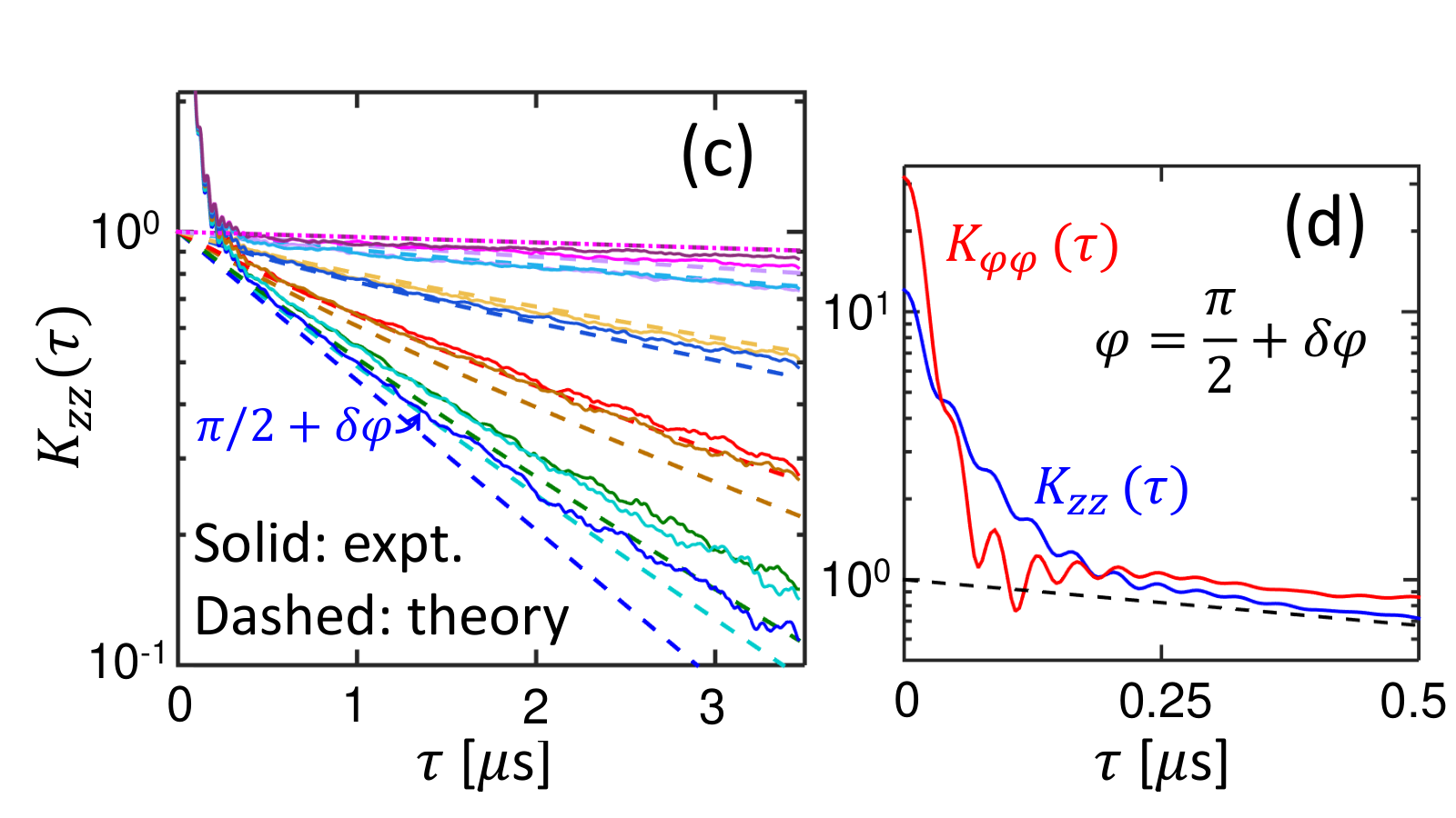
The self-correlator $K_{zz}(\tau)$ as a function of $\tau$ is shown in Fig. 2(c) for 11 values of $\varphi$ (results for $K_{\varphi\varphi}$ are similar). The agreement between the theory (dashed lines) and experiment (solid lines) is good, except for small $\tau$ (discussed below). A significant discrepancy for values of $\varphi$ close to $\pi/2$ is probably caused by remaining offsets $\tilde{I}_{i}^{\rm off}$, which vary from trace to trace. Note that the lines in 2(c) come in pairs, corresponding to angles $\varphi_{n}$ and $\pi-\varphi_{n}$. The separation of the analytical lines in the pairs is due to $\delta\varphi$, while separation of experimental lines is smaller, probably indicating a smaller value of $\delta\varphi$ (partial compensation could be due to imperfect phase matching of applied microwaves or their dispersion in the cable).

Looking at the experimental self-correlators $K_{zz}(\tau)$ and $K_{\varphi\varphi}(\tau)$ at small $\tau$ for $\varphi_{n}=\pi/2$ [Fig. 2(d)], we see that in contrast to the theoretical results, there is a very significant increase of $K_{ii}(\tau)$ at $\tau\lesssim 0.1\,\mu{\rm s}$. The discrepancy is due to the assumption of delta-correlated noise in our theory, while in the experiment the amplifying chain has a finite bandwidth (the Josephson parametric amplifiers have a half-bandwidth of 3.6 MHz and 10 MHz for $\sigma_{z}$ and $\sigma_{\varphi}$ channels, respectively), and the output signals $\tilde{I}_{i}(t)$ are also passed through analog filters with a quite sharp cutoff at $\sim$25 MHz (this cutoff produces clearly visible oscillations with $\sim$40 ns period). Therefore, the theoretical delta-function contribution $\tau_{i}\,\delta(\tau)$ to $K_{ii}(\tau)$ becomes widened in experiment. It is interesting to note that, somewhat counterintuitively, a finite bandwidth of measurement resonator modes does not produce a contribution to $K_{ii}(\tau)$ at $0<\tau\lesssim\kappa_{i}^{-1}$ when $\Gamma_{i}\ll\kappa_{i}$ [38] ($\kappa_{z}^{-1}\approx 37$ ns, $\kappa_{\varphi}^{-1}\approx 22$ ns). This can be understood by considering a resonator without a qubit; then a finite bandwidth $\kappa_{i}$ does not affect the amplified delta-correlated vacuum noise, so that only classical fluctuations of the resonator field (e.g., due to parameter fluctuations or elevated resonator temperature) will produce output fluctuations with $2/\kappa_{i}$ time scale. We have checked that the lines in Fig. 2(d) do not contain noticeable exponential contributions with decay time of $2/\kappa_{i}$ (small expected contributions with amplitude on the order of $\Gamma_{j}/\kappa_{i}$ [38] are below experimental accuracy).

Estimation of residual $\tilde{\Omega}_{\rm R}$.—We now show that the antisymmetrized cross-correlator is a useful tool and can be used to estimate small residual Rabi oscillations frequency $\tilde{\Omega}_{\rm R}$ in the experiment. From Eq. (15) we find

Since in the case $|\tilde{\Omega}_{\rm R}|\ll\Gamma_{z,\varphi}$ we can neglect $\tilde{\Omega}_{\rm R}$ in Eq. (16) for $\Gamma_{\pm}$, Eq. (19) gives a direct way to find $\tilde{\Omega}_{\rm R}$ from the experimental antisymmetrized cross-correlator. The solid line in Fig. 3 shows $K_{z\varphi}(\tau)-K_{\varphi z}(\tau)$ from the experimental data for $\varphi=\pi/2$. Fitting this dependence on $\tau$ with Eq. (19) (dashed line), we find the value $\tilde{\Omega}_{\rm R}/2\pi\approx 12$ kHz, which is within the experimentally expected range of frequency mismatch between $\Omega_{\rm R}$ and $\Omega_{\rm rf}$. Note that the overall shapes of the solid and dashed lines agree well with each other. Estimation of $\tilde{\Omega}_{\rm R}$ via the antisymmetrized cross-correlation is a very sensitive method and can be used to further reduce $|\tilde{\Omega}_{\rm R}|$ in an experiment, in which a direct measurement of 40 MHz Rabi oscillations with a few-kHz accuracy is a difficult task.

Conclusion.—Using the quantum Bayesian theory for a simultaneous measurement of non-commuting qubit observables, we obtained analytical results for the self- and cross-correlators of the output signals from the measurement. Their comparison with experimental results shows a very good agreement. The correlators can be used for sensitive parameter estimation, in particular, to estimate and eliminate the mismatch between the Rabi oscillations and the sideband frequency shift used for measurement.

Acknowledgements.—We thank Justin Dressel and Andrew Jordan for useful discussions. The work was supported by ARO grant No. W911NF-15-0496. L.S.M acknowledges support from the National Science Foundation Graduate Fellowship Grant No. 1106400.

Supplemental material for “Correlators in simultaneous measurement of non-commuting qubit observables”

Supplemental material for “Correlators in simultaneous measurement of non-commuting qubit observables”

References

- [1] K. Kraus, States, effects and operations: fundamental notoins of quantum theory (Springer, Berlin, 1983).
- [2] C. M. Caves, Phys. Rev. D 33, 1643 (1986).
- [3] M. B. Menskii, Phys. Usp. 41, 923 (1998).
- [4] V. P. Belavkin, J. Multivariate Anal. 42, 171 (1992).
- [5] V. B. Braginsky and F. Ya. Khalili, Quantum measurement (Cambridge University Press, Cambridge, UK, 1992).
- [6] Y. Aharonov, D. Z. Albert, and L. Vaidman, Phys. Rev. Lett. 60, 1351 (1988).
- [7] J. Dalibard, Y. Castin, and K. Mølmer, Phys. Rev. Lett. 68, 580 (1992).
- [8] H. J. Carmichael, An open systems approach to quantum optics (Springer, Berlin, 1993).
- [9] H. M. Wiseman and G. J. Milburn, Phys. Rev. A 47, 642 (1993).
- [10] A. N. Korotkov, Phys. Rev. B 60, 5737 (1999).
- [11] N. Katz, M. Ansmann, R. C. Bialczak, E. Lucero, R. McDermott, M. Neeley, M. Steffen, E. M. Weig, A. N. Cleland, J. M. Martinis, and A. N. Korotkov, Science 312, 1498 (2006).
- [12] A. Palacios-Laloy, F. Mallet, F. Nguyen, P. Bertet, D. Vion, D. Esteve, and A. N. Korotkov, Nat. Phys. 6, 442 (2010).
- [13] R. Vijay, C. Macklin, D. H. Slichter, S. J. Weber, K. W. Murch, R. Naik, A. N. Korotkov, and I. Siddiqi, Nature (London) 490, 77 (2012).
- [14] M. Hatridge, S. Shankar, M. Mirrahimi, F. Schackert, K. Geerlings, T. Brecht, K. M. Sliwa, B. Abdo, L. Frunzio, S. M. Girvin, R. J. Schoelkopf, and M. H. Devoret, Science 339, 178 (2013).
- [15] K. W. Murch, S. J. Weber, C. Macklin, and I. Siddiqi, Nature (London) 502, 211 (2013).
- [16] G. de Lange, D. Riste, M. J. Tiggelman, C. Eichler, L. Tornberg, G. Johansson, A. Wallraff, R. N. Schouten, and L. DiCarlo, Phys. Rev. Lett. 112, 080501 (2014).
- [17] P. Campagne-Ibarcq, L. Bretheau, E. Flurin, A. Auffeves, F. Mallet, and B. Huard, Phys. Rev. Lett. 112, 180402 (2014).
- [18] H. M. Wiseman and G. J. Milburn, Phys. Rev. Lett. 70, 548 (1993).
- [19] R. Ruskov and A. N. Korotkov, Phys. Rev. B 66, 041401 (2002).
- [20] C. Sayrin, I. Dotsenko, X. Zhou, B. Peaudecerf, T. Rybarczyk, G. Sebastien, P. Rouchon, M. Mirrahimi, H. Amini, M. Brune, J.-M. Raimond, and S. Haroche, Nature (London) 477, 73 (2011).
- [21] K. Jacobs, Phys. Rev. A 67, 030301(R) (2003).
- [22] R. Ruskov and A. N. Korotkov, Phys. Rev. B 67, 241305(R) (2003).
- [23] D. Risté, M. Dukalski, C. A. Watson, G. de Lange, M. J. Tiggelman, Y. M. Blanter, K. W. Lehnert, R. N. Schouten, and L. DiCarlo, Nature (London) 502, 350 (2013).
- [24] N. Roch, M. E. Schwartz, F. Motzoi, C. Macklin, R. Vijay, A. W. Eddins, A. N. Korotkov, K. B. Whaley, M. Sarovar, and I. Siddiqi, Phys. Rev. Lett. 112, 170501 (2014).
- [25] C. Ahn, A. C. Doherty, and A. J. Landahl, Phys. Rev. A 65, 042301 (2002).
- [26] M. Sarovar, C. Ahn, K. Jacobs, and G. J. Milburn, Phys. Rev. A 69, 052324 (2004).
- [27] E. Arthurs and J. L. Kelly, Bell System Technical Journal 44, 725 (1965).
- [28] P. Busch, Int. J. Theor. Phys. 24, 63 (1985).
- [29] S. Stenholm, Ann. Phys. 218, 233 (1992).
- [30] A. N. Jordan and M. Büttiker, Phys. Rev. Lett. 95, 220401 (2005).
- [31] H. Wei and Yu. V. Nazarov, Phys. Rev. B 78, 045308 (2008).
- [32] R. Ruskov, A. N. Korotkov, and K. Mølmer, Phys. Rev. Lett. 105, 100506 (2010).
- [33] S. Hacohen-Gourgy, L. S. Martin, E. Flurin, V. V. Ramasesh, K. B. Whaley, and I. Siddiqi, Nature (London) 538, 491 (2016).
- [34] D. V. Averin, Phys. Rev. Lett. 88, 207901 (2002).
- [35] H. M. Wiseman and G. J. Milburn, Quantum measurement and control (Cambridge Univ. Press, 2010).
- [36] J. Gambetta, A. Blais, M. Boissonneault, A. A. Houck, D. I. Schuster, and S. M. Girvin, Phys. Rev. A 77, 012112 (2008).
- [37] A. N. Korotkov, Phys. Rev. B 63, 115403 (2001); arXiv:1111.4016; Phys. Rev. A 94, 042326 (2016).
- [38] See Supplemental Material.
- [39] J. Atalaya, M. Bahrami, L. P. Pryadko, and A. N. Korotkov, arXiv:1612.02096.
- [40] A. Chantasri and A. N. Jordan, Phys. Rev. A 92, 032125 (2015).
- [41] A. N. Korotkov, Phys. Rev. B 63, 085312 (2001).
- [42] A. N. Korotkov, Phys. Rev. B 83, 041406 (2011).
- [1] S. Hacohen-Gourgy, L. S. Martin, E. Flurin, V. V. Ramasesh, K. B. Whaley, and I. Siddiqi, Nature (London) 538, 491 (2016).
- [2] A. N. Korotkov, A. N. Korotkov, Phys. Rev. B 60, 5737 (1999); Phys. Rev. B 63, 115403 (2001).
- [3] A. N. Korotkov, arXiv:1111.4016.
- [4] A. N. Korotkov, Phys. Rev. A 94, 042326 (2016).
- [5] H. M. Wiseman and G. J. Milburn, Phys. Rev. A 47, 642 (1993).
- [6] J. Gambetta, A. Blais, M. Boissonneault, A. A. Houck, D. I. Schuster, and S. M. Girvin, Phys. Rev. A 77, 012112 (2008).
- [7] A. Blais, R.-S. Huang, A. Wallraff, S. M. Girvin, and R. J. Schoelkopf, Phys. Rev. A 69, 062320 (2004).
- [8] R. Ruskov, A. N. Korotkov, and K. Mølmer, Phys. Rev. Lett. 105, 100506 (2010).
- [9] A. N. Korotkov, Phys. Rev. B 63, 085312 (2001).
- [10] C. W. Gardiner and P. Zoller, Quantum noise (Springer, Berlin, 2004), Sec. 5.2.
- [11] C. W. Gardiner and M. J. Collett, Phys. Rev. A 31, 3761 (1985).
- [12] A. A. Clerk, M. H. Devoret, S. M. Girvin, F. Marquardt, and R. J. Schoelkopf, Rev. Mod. Phys. 82, 1155 (2010).