跳到论文正文
W Papers独立论文阅读器 arXiv:1702.08064 论文正文 计算阅读时间 · 0%
引用这篇论文根据当前论文元数据生成,正式投稿前建议核对。


License: arXiv.org perpetual non-exclusive license
arXiv:1702.08064v5 [math.PR] 24 Sep 2019
11footnotetext: Zuse Institute Berlin, Takustrasse 7, 14195 Berlin, Germany. Email: wei.zhang@fu-berlin.de

Ergodic SDEs on submanifolds and related numerical sampling schemes

Wei Zhang
Abstract

In many applications, it is often necessary to sample the mean value of certain quantity with respect to a probability measure μ\mu on the level set of a smooth function ξ:ℝd→ℝk\xi:\mathbb{R}^{d}\rightarrow\mathbb{R}^{k}, 1≤k<d1\leq k<d. A specially interesting case is the so-called conditional probability measure, which is useful in the study of free energy calculation and model reduction of diffusion processes. By Birkhoff’s ergodic theorem, one approach to estimate the mean value is to compute the time average along an infinitely long trajectory of an ergodic diffusion process on the level set whose invariant measure is μ\mu. Motivated by the previous work of Ciccotti, Lelièvre, and Vanden-Eijnden [10], as well as the work of Lelièvre, Rousset, and Stoltz [32], in this paper we construct a family of ergodic diffusion processes on the level set of ξ\xi whose invariant measures coincide with the given one. For the conditional measure, we propose a consistent numerical scheme which samples the conditional measure asymptotically. The numerical scheme doesn’t require computing the second derivatives of ξ\xi and the error estimates of its long time sampling efficiency are obtained.

Keywords ergodic diffusion process, reaction coordinate, level set, conditional probability measure

1 Introduction

Many stochastic dynamical systems in real-world applications in physics, chemistry, and biology often involve a large number of degrees of freedom which evolve on vastly different time scales. Understanding the behavior of these systems can be highly challenging due to the high dimensionality and the existence of multiple time scales. To tackle these difficulties, the terminology reaction coordinate, or collective variable, is often introduced to help describe the essential dynamical behavior of complex systems [18, 19, 27, 34, 37].

In various research topics, in particular those related to molecular dynamics, one often encounters the problem of computing the mean value of certain quantity on the level set

Σ=ξ−1​(𝟎)={x∈ℝd|ξ⁡(x)=𝟎∈ℝk}\displaystyle\Sigma=\xi^{-1}(\bm{0})=\Big\{x\in\mathbb{R}^{d}~\Big|~\xi(x)=\bm{0}\in\mathbb{R}^{k}\Big\} (1)

of a reaction coordinate function ξ:ℝd→ℝk\xi:\mathbb{R}^{d}\rightarrow\mathbb{R}^{k}, 1≤k<d1\leq k<d. Among different probability measures on Σ\Sigma, the one defined by

dμ1=1Ze−β​U[det(∇ξT∇ξ)]−12dν\displaystyle d\mu_{1}=\frac{1}{Z}e^{-\beta U}\big[\mbox{det}(\nabla\xi^{T}\nabla\xi)\big]^{-\frac{1}{2}}d\nu (2)

is especially relevant in applications and is sometimes called the conditional probability measure on Σ\Sigma. In (2), the parameter β>0\beta>0, U:ℝd→ℝU:\mathbb{R}^{d}\rightarrow\mathbb{R} is a smooth function, ZZ is the normalization constant, ∇ξ\nabla\xi denotes the d×kd\times k Jacobian matrix of the map ξ\xi, and ν\nu is the surface measure on Σ\Sigma induced from the Lebesgue measure on ℝd\mathbb{R}^{d}. The probability measure μ1\mu_{1} has a probabilistic interpretation, and the numerical computation of the mean value

f¯=∫Σf⁡(x)​d​μ1​(x)\displaystyle\overline{f}=\int_{\Sigma}f(x)\,d\mu_{1}(x) (3)

for a function ff on the level set is involved in various contexts, such as free energy calculations based on the thermodynamics integration formula [31, 32, 20].

Applying Birkhoff’s ergodic theorem, the mean value f¯\overline{f} can be approximated by the time average 1T​∫0Tf⁡(Xs)​𝑑s\frac{1}{T}\int_{0}^{T}f(X_{s})ds along a long trajectory of the process XsX_{s} which evolves on the level set Σ\Sigma and has the invariant measure μ1\mu_{1}. For this purpose, it is helpful to construct a diffusion process on the level set with the correct invariant measure μ1\mu_{1}, i.e., to write down the stochastic differential equation (SDE) of XsX_{s} in ℝd\mathbb{R}^{d}. While finding such a SDE is trivial in the linear reaction coordinate case [42], it is not obvious when the reaction coordinate ξ\xi is a nonlinear function of system’s state.

In the literature, the problem finding SDEs on the level set of the reaction coordinate function with a given invariant measure has been considered in the study of free energy calculations [9, 31, 10, 32]. Given a smooth function U:ℝd→ℝU:\mathbb{R}^{d}\rightarrow\mathbb{R}, the authors in [10] constructed a diffusion process YsY_{s} on Σ\Sigma whose unique invariant measure is μ2\mu_{2}, given by

d​μ2=1Z​e−β​U​d​ν.\displaystyle d\mu_{2}=\frac{1}{Z}e^{-\beta U}d\nu\,. (4)

It is also shown in [10] that this process YsY_{s} can be obtained by projecting the dynamics

d​Y~s\displaystyle d\widetilde{Y}_{s} =−∇U​(Y~s)​d​s+2​β−1​d​Ws\displaystyle=-\nabla U(\widetilde{Y}_{s})\,ds+\sqrt{2\beta^{-1}}dW_{s} (5)

from ℝd\mathbb{R}^{d} onto the level set Σ\Sigma, where Ws=(Ws1,⋯,Wsd)TW_{s}=(W_{s}^{1},\cdots,W_{s}^{d})^{T} is a dd-dimensional Brownian motion. The dynamics YsY_{s} can be used to sample μ2\mu_{2}, and therefore to sample the conditional measure μ1\mu_{1} in (2) as well, by either modifying the potential UU or reweighting the function ff according to the factor [det(∇ξT∇ξ)]−12\big[\mbox{det}(\nabla\xi^{T}\nabla\xi)\big]^{-\frac{1}{2}}. In a more recent work [32], the authors studied the constrained Langevin dynamics, which evolves on the submanifold of the entire phase space including both position and momentum. It is shown in [32] that the position components of the constrained Langevin dynamics has the marginal invariant measure which coincides with μ2\mu_{2}. Therefore, it can also be used to compute the average f¯\overline{f} with respect to the conditional measure μ1\mu_{1} (by either modifying the potential or reweighting ff according to [det(∇ξT∇ξ)]−12\big[\mbox{det}(\nabla\xi^{T}\nabla\xi)\big]^{-\frac{1}{2}}). Detailed studies on the numerical schemes as well as applications of the constrained Langevin dynamics have been carried out in [32].

The same conditional probability measure μ1\mu_{1} in (2), as well as the average f¯\overline{f} in (3), also plays an important role in the study of the effective dynamics of diffusion processes [25, 15, 27, 44]. As a generalization of the dynamics (5), the diffusion process

d​Y~si\displaystyle d\widetilde{Y}^{i}_{s} =−(ai​j∂U∂xj)(Y~s)ds+1β∂ai​j∂xj(Y~s)ds+2​β−1σi​j(Y~s)dWjs,1≤i≤d,\displaystyle=-\Big(a_{ij}\frac{\partial U}{\partial x_{j}}\Big)(\widetilde{Y}_{s})\,ds+\frac{1}{\beta}\frac{\partial a_{ij}}{\partial x_{j}}(\widetilde{Y}_{s})\,ds+\sqrt{2\beta^{-1}}\sigma_{ij}(\widetilde{Y}_{s})\,dW^{j}_{s}\,,\quad 1\leq i\leq d\,, (6)

and its effective dynamics have been considered in [44], where the matrix-valued coefficients σ,a:ℝd→ℝd×d\sigma,a:\mathbb{R}^{d}\rightarrow\mathbb{R}^{d\times d} are related by a=σ​σTa=\sigma\sigma^{T}, such that aa is uniformly positive definite. Notice that, (6) is written in component-wise form with Einstein’s summation convention (the same Einstein’s summation convention will be used throughout this paper, whenever no ambiguity will arise), and it reduces to (5) when σ=a=id\sigma=a=\mbox{id}. The infinitesimal generator of (6) can be written as

ℒ=eβ​Uβ​∂∂xi​(e−β​U​ai​j​∂∂xj).\displaystyle\mathcal{L}=\frac{e^{\beta U}}{\beta}\frac{\partial}{\partial x_{i}}\Big(e^{-\beta U}a_{ij}\frac{\partial}{\partial x_{j}}\Big)\,. (7)

Under mild conditions on UU, it is known that, for any (smooth, uniformly positive definite) coefficient aa, the dynamics (6) has the common unique invariant measure whose probability density is 1Z​e−β​U\frac{1}{Z}e^{-\beta U} with respect to the Lebesgue measure on ℝd\mathbb{R}^{d}.

Motivated by these previous work, in this paper we try to answer the following two questions.

(Q1)   Besides the process constructed in [10] that is closely related to (5), can we obtain other diffusion processes on Σ\Sigma, which are probably related to (6) involving the coefficients σ,a\sigma,a, and have the same invariant measure? In particular, can we construct SDEs on Σ\Sigma whose invariant measure is μ1\mu_{1}?

(Q2)   Numerically, instead of sampling μ2\mu_{2}, can we directly estimate the mean value in (3) with respect to μ1\mu_{1}, preferably with a numerical algorithm that is easy to implement?

The main contributions of the current work are related to the above questions and are summarized below. First, concerning Question (Q1), in Theorem 1 of Section 2, we will construct a family of diffusion processes on Σ\Sigma which sample either μ1\mu_{1} or μ2\mu_{2}. In particular, we show that the diffusion process

d​Xsi=\displaystyle dX_{s}^{i}= −(P​a)i​j​∂U∂xj​d​s+1β​∂(P​a)i​j∂xj​d​s+2​β−1​Pj,i​d​Wsj,1≤i≤d,\displaystyle-(Pa)_{ij}\frac{\partial U}{\partial x_{j}}\,ds+\frac{1}{\beta}\frac{\partial(Pa)_{ij}}{\partial x_{j}}\,ds+\sqrt{2\beta^{-1}}\,P_{j,i}\,dW_{s}^{j}\,,\quad 1\leq i\leq d\,, (8)

evolves on Σ\Sigma and the invariant measure is the conditional probability measure μ1\mu_{1} in (2), where the projection map PP and the invertible k×kk\times k symmetric matrix Ψ\Psi are given by

P=id−a∇ξΨ−1∇ξT,Ψ=∇ξTa∇ξ.\displaystyle P=\mbox{id}-a\nabla\xi\Psi^{-1}\nabla\xi^{T},\quad\Psi=\nabla\xi^{T}a\nabla\xi. (9)

Correspondingly, the infinitesimal generator of (8) is

ℒ=eβ​Uβ​∂∂xi​(e−β​U​(P​a)i​j​∂∂xj),\displaystyle\mathcal{L}=\frac{e^{\beta U}}{\beta}\frac{\partial}{\partial x_{i}}\Big(e^{-\beta U}(Pa)_{ij}\frac{\partial}{\partial x_{j}}\Big)\,, (10)

which should be compared to the infinitesimal generator in (7). Second, concerning Question (Q2), in Section 3 we study a numerical algorithm which estimates the mean value f¯\overline{f} in (3). Specifically, we propose to use the numerical scheme

xi(l+12)=xi(l)+(−ai​j​∂U∂xj+1β​∂ai​j∂xj)​(x(l))​h+2​β−1​h​σi​j​(x(l))​ηj(l),1≤i≤d,x(l+1)=Θ⁡(x(l+12)),\displaystyle\begin{split}x^{(l+\frac{1}{2})}_{i}=&x^{(l)}_{i}+\Big(-a_{ij}\frac{\partial U}{\partial x_{j}}+\frac{1}{\beta}\frac{\partial a_{ij}}{\partial x_{j}}\Big)(x^{(l)})\,h+\sqrt{2\beta^{-1}h}\,\sigma_{ij}(x^{(l)})\,\eta^{(l)}_{j}\,,\quad 1\leq i\leq d\,,\\ x^{(l+1)}=&\Theta\big(x^{(l+\frac{1}{2})}\big)\,,\end{split} (11)

with x(0)∈Σx^{(0)}\in\Sigma, and to approximate f¯\overline{f} by f^n=1n​∑l=0n−1f⁡(x(l))\widehat{f}_{n}=\frac{1}{n}\sum\limits_{l=0}^{n-1}f(x^{(l)}). In (11), hh is the step-size, 𝜼(l)=(η1(l),η2(l),⋯,ηd(l))T\bm{\eta}^{(l)}=(\eta_{1}^{(l)},\eta_{2}^{(l)},\cdots,\eta_{d}^{(l)})^{T} are independent dd-dimensional standard Gaussian random variables, and Θ⁡(x)=lims→+∞φ⁡(x,s)\Theta(x)=\lim\limits_{s\rightarrow+\infty}\varphi(x,s) is the limit of the flow map

d​φ​(x,s)d​s=−(a∇F)(φ(x,s)),φ(x,0)=x,∀x∈ℝd,\displaystyle\begin{split}\frac{d\varphi(x,s)}{ds}=&-(a\nabla F)\big(\varphi(x,s)\big)\,,\quad\varphi(x,0)=x,\qquad\forall~x\in\mathbb{R}^{d}\,,\end{split} (12)

with F⁡(x)=12​|ξ⁡(x)|2=12​∑α=1kξα2​(x)F(x)=\frac{1}{2}|\xi(x)|^{2}=\frac{1}{2}\sum\limits_{\alpha=1}^{k}\xi_{\alpha}^{2}(x). Following the approach developed in [36], in Theorem 2, we obtain the estimates of the approximation error between f^n\widehat{f}_{n} and f¯\overline{f}. While different constraint approaches have been proposed in the literature [28, 32, 43], to the best of the author’s knowledge, constraint using the flow map φ\varphi has not been studied yet.

Let us comment on the two contributions mentioned above. First, knowing the SDE (8) and the expression (10) of its infinitesimal generator ℒ\mathcal{L} is helpful for analysis. In fact, in Section 3, the analysis of sampling error estimate of the scheme (11) relies on Poisson equation on Σ\Sigma related to ℒ\mathcal{L} in (10). Furthermore, (10) plays a role in the work [30] in analyzing the approximation quality of the effective dynamics, while SDE (8) has been used in [20] to study fluctuation relations and Jarzynski’s equality for nonequilibrium systems. Second, we emphasize that Θ⁡(x)\Theta(x) in the scheme (11) can be evaluated by solving the ODE (12) starting from xx. Although Θ\Theta is defined as the limit when s→+∞s\rightarrow+\infty, in many cases the computational cost is not large, due to the exponential convergence of the (gradient) flow (12) to its limit, particularly for the initial state x=x(l+12)x=x^{(l+\frac{1}{2})} that is close to Σ\Sigma. Furthermore, comparing to the direct (Euler-Maruyama) discretization of SDE (8) which may deviate from Σ\Sigma and requires second order derivatives of ξ\xi, the scheme (11) satisfies x(l)∈Σx^{(l)}\in\Sigma for all l≥0l\geq 0, and it doesn’t require computing the second order derivatives of ξ\xi. Therefore, we expect the numerical scheme (11)–(12) is both stable and relatively easy to implement. Readers are referred to Remark 4–5 in Section 3 and Example 11 in Section 4 for further algorithmic discussions.

In the following, we briefly explain the approach that we will use to study Question (Q1), as well as the idea behind the scheme (11)–(12). Concerning Question (Q1), we take the manifold point of view by considering ℝd\mathbb{R}^{d} as a Riemannian manifold ℳ=(ℝd,g)\mathcal{M}=(\mathbb{R}^{d},g) with the metric g=a−1g=a^{-1}, defined by

g⁡(𝒖,𝒗)=⟨𝒖,𝒗⟩g=ui​(a−1)i​j​vj,∀𝒖,𝒗∈ℝd.\displaystyle g(\bm{u},\bm{v})=\langle\bm{u},\bm{v}\rangle_{g}=u_{i}(a^{-1})_{ij}v_{j}\,,\quad\forall~\bm{u},\bm{v}\in\mathbb{R}^{d}\,. (13)

A useful observation is that, for ℒ\mathcal{L} in (7), we have [44]

ℒ​f\displaystyle\mathcal{L}f =[−gradℳ​(U+12​β​ln⁡G)+1β​Δℳ]​f,∀smooth​f:ℝd→ℝ,\displaystyle=\Big[-\mbox{grad}^{\mathcal{M}}\Big(U+\frac{1}{2\beta}\ln G\Big)+\frac{1}{\beta}\Delta^{\mathcal{M}}\Big]f\,,\quad\forall~\mbox{smooth}~f:\mathbb{R}^{d}\rightarrow\mathbb{R}\,,

where G=det​gG=\mbox{det}g, and gradℳ\mbox{grad}^{\mathcal{M}}, Δℳ\Delta^{\mathcal{M}} denote the gradient and the Laplacian-Beltrami operator on ℳ\mathcal{M}, respectively. Accordingly, (6) can be written as a SDE on ℳ\mathcal{M} as

d​Y~s=−gradℳ​(U+12​β​ln⁡G)​d​s+2​β−1​d​B~s,\displaystyle d\widetilde{Y}_{s}=-\mbox{grad}^{\mathcal{M}}\Big(U+\frac{1}{2\beta}\ln G\Big)\,ds+\sqrt{2\beta^{-1}}d\widetilde{B}_{s}\,, (14)

where B~s\widetilde{B}_{s} is the Brownian motion on ℳ\mathcal{M} [21]. Conversely, SDE (6) can be seen as the equation of (14) under the (global) coordinate chart of ℳ\mathcal{M}. This equivalence allows us to study (6) on ℝd\mathbb{R}^{d} by the corresponding SDE (14) on manifold ℳ\mathcal{M}. Comparing to (6), one advantage of working with the abstract equation (14) is that the invariant measure of (14) can be recognized as easily as in (5), provided that we apply integration by parts formula on the manifold ℳ\mathcal{M}.

A family of ergodic SDEs on Σ\Sigma (i.e., Question (Q1)) is obtained by taking the same manifold point of view. Specifically, consider Σ\Sigma as a submanifold of ℳ\mathcal{M} and denote by gradΣ\mbox{grad}^{\Sigma}, ΔΣ\Delta^{\Sigma}, BsB_{s} the gradient operator, the Laplacian and the Brownian motion (with generator 12​ΔΣ\frac{1}{2}\Delta^{\Sigma} [21]) on Σ\Sigma, respectively. Since the infinitesimal generator of the SDE

d​Ys=−gradΣ​U​d​s+2​β−1​d​Bs\displaystyle dY_{s}=-\mbox{grad}^{\Sigma}Uds+\sqrt{2\beta^{-1}}dB_{s} (15)

is ℒ=−gradΣ​U+1β​ΔΣ\mathcal{L}=-\mbox{grad}^{\Sigma}U+\frac{1}{\beta}\Delta^{\Sigma}, under mild assumptions on UU, it is straightforward to verify that dynamics (15) evolves on Σ\Sigma and has the unique invariant measure 1Z​e−β​U​d​νg\frac{1}{Z}e^{-\beta U}d\nu_{g}, where νg\nu_{g} is the surface measure on Σ\Sigma induced from the metric g=a−1g=a^{-1} on ℳ=(ℝd,g)\mathcal{M}=(\mathbb{R}^{d},g). Therefore, answering Question (Q1) boils down to calculating the expression of (15) under the coordinate chart of ℳ\mathcal{M} (not Σ\Sigma). This will be achieved by calculating the expressions of gradΣ\mbox{grad}^{\Sigma}, ΔΣ\Delta^{\Sigma} under the coordinate chart of ℳ\mathcal{M} and then figuring out the relation between the two measures ν\nu and νg\nu_{g}.

Concerning the idea behind the numerical scheme (11)–(12), we recall that one way to (approximately) sample μ1\mu_{1} on Σ\Sigma is to constrain the dynamics (6) in the neighborhood of Σ\Sigma by adding an extra potential to it. This is often termed as softly constrained dynamics [10, 35] and has been widely used in applications. In this context, one consider the dynamics

d​Xsϵ,i\displaystyle dX^{\epsilon,i}_{s} =[−ai​j​∂U∂xj−1ϵ​ai​j​∂∂xj​(12​∑α=1kξα2)+1β​∂ai​j∂xj]​d​s+2​β−1​σi​j​d​Wsj,\displaystyle=\Big[-a_{ij}\frac{\partial U}{\partial x_{j}}\,-\frac{1}{\epsilon}a_{ij}\frac{\partial}{\partial x_{j}}\Big(\frac{1}{2}\sum\limits_{\alpha=1}^{k}\xi_{\alpha}^{2}\Big)\,+\frac{1}{\beta}\frac{\partial a_{ij}}{\partial x_{j}}\Big]\,ds+\sqrt{2\beta^{-1}}\sigma_{ij}\,dW^{j}_{s}\,, (16)

where ϵ>0\epsilon>0, 1≤i≤d1\leq i\leq d, based on the fact that the invariant measure of (16) converges weakly to μ1\mu_{1}, as ϵ→0\epsilon\rightarrow 0. The dynamics (16) stays close to Σ\Sigma most of the time, thanks to the existence of the extra constraint force. Furthermore, only the first order derivatives of ξ\xi are involved. In spite of these nice properties, however, direct simulation of (16) is inefficient when ϵ\epsilon is small, because the time step-size in numerical simulations becomes severely limited due to the strong stiffness in the dynamics. Indeed, our numerical scheme is motivated in order to overcome the aforementioned drawback of the softly constrained dynamics (16), and the scheme (11)–(12) can be viewed as a multiscale numerical method for (16), where the stiff and non-stiff terms in (16) are handled separately [42]. In contrast to the previous work [23, 14, 10], where the convergence of (16) was studied on a finite time interval, our result concerns the long time sampling efficiency of the discretized numerical scheme.

Before concluding this introduction, we compare the current work with several previous ones. Generally speaking, Monte Carlo samplers (based on ergodicity) either on ℝd\mathbb{R}^{d} or on its submanifolds can be classified into Metropolis-adjusted samplers and samplers without Metropolis step (unadjusted). For Metropolis-adjusted methods, in particular, exploiting Riemannian geometry structure to develop MCMC methods has been studied in [17]. The authors there demonstrated that incorporating the geometry of the space into numerical methods can lead to significant improvement of the sampling efficiency. In line with this development, in Section 4 we will consider a concrete example where a non-constant matrix aa can help remove the stiffness in the sampling task. On the other hand, despite of the common Riemannian manifold point of view in the current work and in [17], the main difference is that the current work deals with sampling on the submanifold Σ\Sigma instead of the entire ℝd\mathbb{R}^{d} (or its domain). The derivations in the current work are more involved mainly due to this difference. Besides sampling on the entire space, Metropolis-adjusted samplers on submanifolds, using either MCMC or Hybrid Monte Carlo, have been considered in several recent work [8, 32, 43, 33]. Reversible Metropolis random walk on submanifolds has been constructed in [43], which is then extended in [33] by allowing non-zero gradient forces in the proposal move. In contrast to these Metropolis-adjusted samplers, the numerical scheme (11)–(12) in the current work is unadjusted (without Metropolis-step) and samples the conditional probability measure μ1\mu_{1} when the step-size h→0h\rightarrow 0. This means that in practice the step-size hh should be chosen properly such that the discretization error is tolerable. In this direction, we point out that unadjusted samplers on ℝd\mathbb{R}^{d}, which naturally arise from discretizations of SDEs, have been well studied in the literature [41, 29, 7, 11, 1, 36]. The current work can be thought as a further step along this direction for sampling schemes on submanifolds, by applying the machinery developed in [36]. Comparison between the scheme (11) and the Metropolis-adjusted algorithm in [43] can be found in Remark 8, as well as in Example 22 in Section 4. We also refer to [29] for related discussions.

The rest of the paper is organized as follows. In Section 2, we construct ergodic SDEs on Σ\Sigma which sample either μ1\mu_{1} or μ2\mu_{2}. In Section 3, we study the numerical scheme (11)–(12) and quantify its approximation error in estimating the mean value in (3). In Section 4, we demonstrate our results through concrete examples. Conclusions and further discussions are made in Section 5. Technical details related to the Riemannian manifold ℳ\mathcal{M} in Section 2 are included in Appendix A. Proofs of the results in Section 3 are collected in Appendix B.

Finally, we conclude this introduction with the assumptions which will be made (implicitly) throughout this paper.

Assumption 1.

The matrix σ:ℝd→ℝd×d\sigma:\mathbb{R}^{d}\rightarrow\mathbb{R}^{d\times d} is both smooth and invertible at each x∈ℝdx\in\mathbb{R}^{d}. The matrix a=σ​σTa=\sigma\sigma^{T} is uniformly positive definite with uniformly bounded inverse a−1a^{-1}.

Assumption 2.

The function ξ:ℝd→ℝk\xi:\mathbb{R}^{d}\rightarrow\mathbb{R}^{k} is C2C^{2} smooth and the level set Σ\Sigma is both connected and compact, such that rank​(∇ξ)=k\mbox{rank}(\nabla\xi)=k at each x∈Σx\in\Sigma.

2 SDEs of ergodic diffusion processes on Σ\Sigma

In this section, we construct SDEs of ergodic processes on Σ\Sigma that sample a given invariant measure. The main result of this section is Theorem 1, which shows that the invariant measure of the SDE (8) in Introduction is the conditional probability measure μ1\mu_{1} in (2). Readers who are mainly interested in numerical algorithms can read Theorem 1 and then directly jump to Section 3.

First of all, let us point out that, the semigroup approach based on functional inequalities on Riemannian manifolds is well developed to study the solution of Fokker-Planck equation towards equilibrium. One sufficient condition for the exponential convergence of the Fokker-Planck equation (and therefore the ergodicity of the corresponding dynamics) is the famous Bakry-Emery criterion [4]. In particular, concrete conditions are given in [40] which guarantee the exponential convergence to the unique invariant measure. In the following, we will always assume that the potential U∈C∞​(Σ)U\in C^{\infty}(\Sigma) and the Bakry-Emery condition in [40] is satisfied.

Recall that ℳ=(ℝd,g)\mathcal{M}=(\mathbb{R}^{d},g), where g=a−1g=a^{-1} and νg\nu_{g} is the surface measure on Σ\Sigma induced from ℳ\mathcal{M}. Matrices PP, Pj,iP_{j,i} are given in (77), (80) in Appendix A, respectively. For 1≤i≤d1\leq i\leq d, 𝒆i\bm{e}_{i} denotes the vector whose iith component equals to 11 while all the other d−1d-1 components equal to 00. We refer the reader to Appendix A for further details. Let us first consider the probability measure μ\mu on Σ\Sigma given by d​μ=1Z​e−β​U​d​νgd\mu=\frac{1}{Z}e^{-\beta U}d\nu_{g}, where β>0\beta>0 and ZZ is a normalization constant. The following proposition is a direct application of Proposition 5 in Appendix A.

Proposition 1.

Consider the dynamics on ℝd\mathbb{R}^{d} which satisfies the Ito SDE

d​Ysi=−(P​a)i​j​∂[U−12​βln((deta)−1det(∇ξTa∇ξ))]∂xj​d​s+1β​∂(P​a)i​j∂xj​d​s+2​β−1​Pj,i​d​Wsj\displaystyle\begin{split}dY_{s}^{i}=&-(Pa)_{ij}\frac{\partial\big[U-\frac{1}{2\beta}\ln\big((\det a)^{-1}\det(\nabla\xi^{T}a\nabla\xi)\big)\big]}{\partial x_{j}}\,ds+\frac{1}{\beta}\frac{\partial(Pa)_{ij}}{\partial x_{j}}\,ds+\sqrt{2\beta^{-1}}\,P_{j,i}\,dW_{s}^{j}\end{split} (17)

for 1≤i≤d1\leq i\leq d, where Ws=(Ws1,Ws2,⋯,Wsd)TW_{s}=(W_{s}^{1},W_{s}^{2},\cdots,W_{s}^{d})^{T} is a dd-dimensional Brownian motion. Suppose Y0∈ΣY_{0}\in\Sigma, then Ys∈ΣY_{s}\in\Sigma almost surely for s≥0s\geq 0. Furthermore, it has a unique invariant measure μ\mu given by d​μ=1Z​e−β​U​d​νgd\mu=\frac{1}{Z}e^{-\beta U}d\nu_{g}.

Proof.

Using (80) and Proposition 5 in Appendix A, we know that the infinitesimal generator of SDE (17) is

ℒ​f=−⟨gradΣ​U,gradΣ​f⟩g+1β​ΔΣ​f,∀f:Σ→ℝ,\displaystyle\mathcal{L}f=-\langle\mbox{grad}^{\Sigma}U,\mbox{grad}^{\Sigma}f\rangle_{g}+\frac{1}{\beta}\Delta^{\Sigma}f\,,\quad\forall~f:\Sigma\rightarrow\mathbb{R}\,, (18)

where gradΣ\mbox{grad}^{\Sigma}, ΔΣ\Delta^{\Sigma} are the gradient and Laplace-Beltrami operators on Σ\Sigma of ℳ\mathcal{M}, respectively. Applying Ito’s formula to ξα​(Ys)\xi_{\alpha}(Y_{s}), we have

d​ξα​(Ys)=ℒ​ξα​(Ys)​d​s+2​β−1​∂ξα​(Ys)∂xi​Pj,i​d​Wsj,1≤α≤k.\displaystyle d\xi_{\alpha}(Y_{s})=\mathcal{L}\xi_{\alpha}(Y_{s})\,ds+\sqrt{2\beta^{-1}}\frac{\partial\xi_{\alpha}(Y_{s})}{\partial x_{i}}P_{j,i}dW_{s}^{j}\,,\quad 1\leq\alpha\leq k\,.

Using (18), (80) in Appendix A, and the fact that gradΣ​ξα=P​gradℳ​ξα=0\mbox{grad}^{\Sigma}\xi_{\alpha}=P\mbox{grad}^{\mathcal{M}}\xi_{\alpha}=0, it is straightforward to verify that

ℒ​ξα=−⟨gradΣ​U,gradΣ​ξα⟩g+1β​divΣ​(gradΣ​ξα)=0,\displaystyle\mathcal{L}\xi_{\alpha}=-\langle\mbox{grad}^{\Sigma}U,\mbox{grad}^{\Sigma}\xi_{\alpha}\rangle_{g}+\frac{1}{\beta}\mbox{div}^{\Sigma}(\mbox{grad}^{\Sigma}\xi_{\alpha})=0\,,
∂ξα∂xi​Pj,i=0,1≤j≤d,\displaystyle\frac{\partial\xi_{\alpha}}{\partial x_{i}}P_{j,i}=0\,,\quad 1\leq j\leq d\,,

on Σ\Sigma, which implies d​ξα​(Ys)=0d\xi_{\alpha}(Y_{s})=0, ∀s≥0\forall s\geq 0. Since Y0∈ΣY_{0}\in\Sigma, we conclude that ξα​(Ys)=ξα​(Y0)=0\xi_{\alpha}(Y_{s})=\xi_{\alpha}(Y_{0})=0 a.s. s≥0s\geq 0, for 1≤α≤k1\leq\alpha\leq k, and therefore Ys∈ΣY_{s}\in\Sigma for s≥0s\geq 0, almost surely.

Using the expression (18) of ℒ\mathcal{L} and the integration by parts formula (85) in Appendix A, it is easy to see that μ\mu is an invariant measure of the dynamics (17). The uniqueness is implied by the exponential convergence result established in [40, Remark 1.1 and Corollary 1.5], since we assume Bakry-Emery condition is satisfied. ∎

In the above, we have considered the level set Σ\Sigma as a submanifold of ℳ=(ℝd,g)\mathcal{M}=(\mathbb{R}^{d},g). In applications, on the other hand, it is natural to view Σ\Sigma as a submanifold of the standard Euclidean space ℝd\mathbb{R}^{d}, with the surface measure ν\nu on Σ\Sigma that is induced from the Euclidean metric on ℝd\mathbb{R}^{d}. As already mentioned in the Introduction, the following two probability measures

dμ1=1Ze−β​U[det(∇ξT∇ξ)]−12dν,dμ2=1Ze−β​Udν,\displaystyle d\mu_{1}=\frac{1}{Z}e^{-\beta U}\big[\mbox{det}(\nabla\xi^{T}\nabla\xi)\big]^{-\frac{1}{2}}d\nu\,,\qquad d\mu_{2}=\frac{1}{Z}e^{-\beta U}d\nu, (19)

where ZZ denotes possibly different normalization constants, are often interesting and arise in many situations [9, 10, 27, 44]. In particular, μ1\mu_{1} has a probabilistic interpretation and often appears in the study of free energy calculation and model reduction of stochastic dynamics [31, 27]. In order to construct processes which sample μ1\mu_{1} or μ2\mu_{2}, we need to figure out the relations between the two surface measures νg\nu_{g} and ν\nu on Σ\Sigma.

Lemma 1.

Let νg\nu_{g}, ν\nu be the surface measures on Σ\Sigma induced from the metric g=a−1g=a^{-1} and the Euclidean metric on ℝd\mathbb{R}^{d}, respectively. We have

d​νg=(deta)−12​[det(∇ξTa∇ξ)det(∇ξT∇ξ)]12​d​ν.\displaystyle d\nu_{g}=(\det a)^{-\frac{1}{2}}\bigg[\frac{\mbox{{det}}(\nabla\xi^{T}a\nabla\xi)}{\mbox{{det}}(\nabla\xi^{T}\nabla\xi)}\bigg]^{\frac{1}{2}}d\nu\,.
Proof.

Let x∈Σx\in\Sigma and 𝒗1,𝒗2,⋯,𝒗d−k\bm{v}_{1},\bm{v}_{2},\cdots,\bm{v}_{d-k} be a basis of Tx​ΣT_{x}\Sigma. Assume that 𝒗i=ci​j​𝒆j\bm{v}_{i}=c_{ij}\bm{e}_{j}, where c=(ci​j)c=(c_{ij}) is a (d−k)×d(d-k)\times d matrix whose rank is d−kd-k. Using the fact ⟨𝒗i,gradℳ​ξα⟩g=0\langle\bm{v}_{i},\mbox{grad}^{\mathcal{M}}\xi_{\alpha}\rangle_{g}=0 for 1≤i≤d−k1\leq i\leq d-k, 1≤α≤k1\leq\alpha\leq k, we can deduce that c∇ξ=0c\,\nabla\xi=0. Calculating the surface measures νg\nu_{g} and ν\nu under this basis, we obtain

d​νg=[det​(c​a−1​cT)det​(c​cT)]12​d​ν.\displaystyle d\nu_{g}=\bigg[\frac{\mbox{det}(ca^{-1}c^{T})}{\mbox{det}(cc^{T})}\bigg]^{\frac{1}{2}}d\nu\,. (20)

To simplify the right hand side of (20), we use the following equality

(c∇ξTa)​(cT∇ξ)=(c​cT0∇ξTacT∇ξTa∇ξ)=(c​a−1∇ξT)​a​(cT∇ξ).\displaystyle\begin{pmatrix}c\\ \nabla\xi^{T}\,a\end{pmatrix}\begin{pmatrix}c^{T}&\nabla\xi\end{pmatrix}=\begin{pmatrix}cc^{T}&0\\ \nabla\xi^{T}ac^{T}&\nabla\xi^{T}a\nabla\xi\end{pmatrix}=\begin{pmatrix}ca^{-1}\\ \nabla\xi^{T}\end{pmatrix}a\begin{pmatrix}c^{T}&\nabla\xi\end{pmatrix}\,.

After computing the determinants of the last two matrices above, we obtain

det(ccT)det(∇ξTa∇ξ)=(deta)det[(c​a−1∇ξT)(cT∇ξ)]=(deta)det(c​a−1​cTca−1∇ξ0∇ξT∇ξ).\displaystyle\det(cc^{T})\,\det(\nabla\xi^{T}a\nabla\xi)=(\det a)\,\det\bigg[\begin{pmatrix}ca^{-1}\\ \nabla\xi^{T}\end{pmatrix}\begin{pmatrix}c^{T}&\nabla\xi\end{pmatrix}\bigg]=(\det a)\,~\det\begin{pmatrix}ca^{-1}c^{T}&ca^{-1}\nabla\xi\\ 0&\nabla\xi^{T}\nabla\xi\end{pmatrix}\,.

The conclusion follows after we substitute the above relation into (20). ∎

Applying Lemma 1 and Proposition 1, we can obtain ergodic processes whose invariant measures are given in (19).

Theorem 1.

Let μ1,μ2\mu_{1},\mu_{2} be the two probability measures on Σ\Sigma defined in (19). Consider the dynamics XsX_{s}, YsY_{s} on ℝd\mathbb{R}^{d} which satisfy the Ito SDEs

d​Xsi=−(P​a)i​j​∂U∂xj​d​s+1β​∂(P​a)i​j∂xj​d​s+2​β−1​Pj,i​d​Wsj,\displaystyle\begin{split}dX_{s}^{i}=&-(Pa)_{ij}\frac{\partial U}{\partial x_{j}}\,ds+\frac{1}{\beta}\frac{\partial(Pa)_{ij}}{\partial x_{j}}\,ds+\sqrt{2\beta^{-1}}\,P_{j,i}\,dW_{s}^{j}\,,\end{split} (21)

and

d​Ysi=−(P​a)i​j​∂[U−12​βlndet(∇ξT∇ξ)]∂xj​d​s+1β​∂(P​a)i​j∂xj​d​s+2​β−1​Pj,i​d​Wsj,\displaystyle\begin{split}dY_{s}^{i}=&-(Pa)_{ij}\frac{\partial\big[U-\frac{1}{2\beta}\ln\det(\nabla\xi^{T}\nabla\xi)\big]}{\partial x_{j}}\,ds+\frac{1}{\beta}\frac{\partial(Pa)_{ij}}{\partial x_{j}}\,ds+\sqrt{2\beta^{-1}}\,P_{j,i}\,dW_{s}^{j}\,,\end{split} (22)

for 1≤i≤d1\leq i\leq d, where β>0\beta>0 and Ws=(Ws1,Ws2,⋯,Wsd)TW_{s}=(W_{s}^{1},W_{s}^{2},\cdots,W_{s}^{d})^{T} is a dd-dimensional Brownian motion. Suppose that X0,Y0∈ΣX_{0},Y_{0}\in\Sigma, then Xs,Ys∈ΣX_{s},Y_{s}\in\Sigma almost surely for s≥0s\geq 0. Furthermore, the unique invariant probability measures of the dynamics XsX_{s} and YsY_{s} are μ1\mu_{1} and μ2\mu_{2}, respectively.

Proof.

Applying Lemma 1, we can rewrite the probability measures μ1,μ2\mu_{1},\mu_{2} as

dμ1=1Ze−β​U[det(∇ξT∇ξ)]−12dν=1Zexp[−β(U+12​βlndet(∇ξTa∇ξ)deta)]dνg,d​μ2=1Z​e−β​U​d​ν=1Z​exp​[−β⁡(U+12​β​ln⁡det(∇ξTa∇ξ)(deta)det(∇ξT∇ξ))]​d​νg,\displaystyle\begin{split}&d\mu_{1}=\frac{1}{Z}e^{-\beta U}\big[\mbox{det}(\nabla\xi^{T}\nabla\xi)\big]^{-\frac{1}{2}}d\nu=\frac{1}{Z}\mbox{exp}\Big[-\beta\Big(U+\frac{1}{2\beta}\ln\frac{\det(\nabla\xi^{T}a\nabla\xi)}{\det a}\Big)\Big]d\nu_{g}\,,\\ &d\mu_{2}=\frac{1}{Z}e^{-\beta U}d\nu=\frac{1}{Z}\mbox{exp}\Big[-\beta\Big(U+\frac{1}{2\beta}\ln\frac{\det\big(\nabla\xi^{T}a\nabla\xi\big)}{(\det a)\det(\nabla\xi^{T}\nabla\xi)}\Big)\Big]d\nu_{g}\,,\end{split} (23)

where again ZZ denotes different normalization constants. Applying Proposition 1 to the two probability measures expressed in (23), we can conclude that both the dynamics XsX_{s} in (21) and YsY_{s} in (22) evolve on the submanifold Σ\Sigma, and their invariant probability measures are given by μ1\mu_{1} and μ2\mu_{2}, respectively. ∎

Remark 1.

Under Assumptions 1–2, we can find a neighborhood 𝒪\mathcal{O} of Σ\Sigma, such that PP can be extended to 𝒪\mathcal{O}. Furthermore, the relations in (79) in Appendix A are still satisfied in 𝒪\mathcal{O}. Due to this fact, in (22)–(22) we can talk about the derivatives of PP at states x∈Σx\in\Sigma.

Remark 2.
  1. 1.

    Notice that, similar to (7), the infinitesimal generator of XsX_{s} in (21) can be written as

    ℒ=eβ​Uβ​∂∂xi​(e−β​U​(P​a)i​j​∂∂xj).\displaystyle\mathcal{L}=\frac{e^{\beta U}}{\beta}\frac{\partial}{\partial x_{i}}\Big(e^{-\beta U}(Pa)_{ij}\frac{\partial}{\partial x_{j}}\Big)\,. (24)

    Using (23) and (85) in Appendix A, we can also verify the integration by parts formula

    ∫Σ(ℒf)f′dμ1=∫Σ(ℒf′)fdμ1=−1β∫Σ(Pa∇f)⋅∇f′dμ1,\displaystyle\int_{\Sigma}(\mathcal{L}f)f^{\prime}\,d\mu_{1}=\int_{\Sigma}(\mathcal{L}f^{\prime})f\,d\mu_{1}=-\frac{1}{\beta}\int_{\Sigma}(Pa\nabla f)\cdot\nabla f^{\prime}\,d\mu_{1}\,, (25)

    for any two C2C^{2} smooth functions f,f′:Σ→ℝf,f^{\prime}:\Sigma\rightarrow\mathbb{R}.

  2. 2.

    Using Jacobi’s formula [38] ∂lndet(∇ξT∇ξ)∂xj=(∇ξT∇ξ)α​η−1∂(∇ξαT∇ξη)∂xj\frac{\partial\ln\det(\nabla\xi^{T}\nabla\xi)}{\partial x_{j}}=(\nabla\xi^{T}\nabla\xi)^{-1}_{\alpha\eta}\frac{\partial(\nabla\xi_{\alpha}^{T}\nabla\xi_{\eta})}{\partial x_{j}} and (P​a)i​j​∂jξα=0(Pa)_{ij}\partial_{j}\xi_{\alpha}=0, the equation (22) can be simplified as

    d​Ysi=\displaystyle dY_{s}^{i}= −(P​a)i​j​∂U∂xj​d​s+1β​Qj​l​∂(P​a)i​j∂xl​d​s+2​β−1​Pj,i​d​Wsj,\displaystyle-(Pa)_{ij}\frac{\partial U}{\partial x_{j}}\,ds+\frac{1}{\beta}Q_{jl}\frac{\partial(Pa)_{ij}}{\partial x_{l}}\,ds+\sqrt{2\beta^{-1}}\,P_{j,i}\,dW_{s}^{j}\,,

    where the matrix Q=id−∇ξ(∇ξT∇ξ)−1∇ξTQ=\mbox{id}-\nabla\xi(\nabla\xi^{T}\nabla\xi)^{-1}\nabla\xi^{T}. In the special case when g=a=idg=a=\mbox{{id}}, we have νg=ν\nu_{g}=\nu and Pj,i=Pj​i=Qj​iP_{j,i}=P_{ji}=Q_{ji} from (80). Accordingly, we can write the dynamics (22) as

    d​Ysi=−Pi​j​∂U∂xj​d​s+1β​Pl​j​∂Pl​i∂xj​d​s+2​β−1​Pj​i​d​Wsj=−Pi​j​∂U∂xj​d​s−1β​(Ψ−1)α​γ​Pl​j​(∂l​j2ξα)​∂iξγ​d​s+2​β−1​Pj​i​d​Wsj,=−Pi​j​∂U∂xj​d​s+1β​Hi​d​s+2​β−1​Pj​i​d​Wsj,\displaystyle\begin{split}dY_{s}^{i}=&-P_{ij}\frac{\partial U}{\partial x_{j}}\,ds+\frac{1}{\beta}P_{lj}\frac{\partial P_{li}}{\partial x_{j}}\,ds+\sqrt{2\beta^{-1}}\,P_{ji}\,dW_{s}^{j}\\ =&-P_{ij}\frac{\partial U}{\partial x_{j}}\,ds-\frac{1}{\beta}(\Psi^{-1})_{\alpha\gamma}P_{lj}(\partial^{2}_{lj}\xi_{\alpha})\partial_{i}\xi_{\gamma}\,ds+\sqrt{2\beta^{-1}}\,P_{ji}\,dW_{s}^{j}\,,\\ =&-P_{ij}\frac{\partial U}{\partial x_{j}}\,ds+\frac{1}{\beta}H_{i}ds+\sqrt{2\beta^{-1}}\,P_{ji}\,dW_{s}^{j}\,,\end{split} (26)

    for 1≤i≤d1\leq i\leq d, where H=Hi​𝒆iH=H_{i}\bm{e}_{i} is the mean curvature vector of Σ\Sigma (see Proposition 4 in Appendix A). In Stratonovich form, (26) can be written as

    d​Ysi=\displaystyle dY_{s}^{i}= −Pi​j​∂U∂xj​d​s+2​β−1​Pj​i∘d​Wsj,1≤i≤d.\displaystyle-P_{ij}\frac{\partial U}{\partial x_{j}}ds+\sqrt{2\beta^{-1}}P_{ji}\circ\,dW_{s}^{j}\,,\hskip 5.69046pt1\leq i\leq d\,. (27)

    In this case, our results are accordant with those in [10].

The dynamics constructed in Proposition 1 and Theorem 1 are reversible on Σ\Sigma, in the sense that their infinitesimal generators are self-adjoint with respect to their invariant measures. In fact, using the same idea, we can construct non-reversible ergodic SDEs on Σ\Sigma as well. We will only consider the conditional probability measure μ1\mu_{1}, since it is more relevant in applications and the result is also simpler.

Corollary 1.

Let μ1\mu_{1} be the conditional probability measure on Σ\Sigma defined in (19). The vector field 𝐉=(J1,J2,⋯,Jd)T=Ji​𝐞i\bm{J}=(J_{1},J_{2},\cdots,J_{d})^{T}=J_{i}\bm{e}_{i}, defined on x∈Σx\in\Sigma, satisfies

𝑱(x)∈TxΣ,∀x∈Σ,Pi​j​∂Jj∂xi+Jj​∂Pi​j∂xi−β​Ji​∂U∂xi=0.\displaystyle\begin{split}\bm{J}(x)\in T_{x}\Sigma,\qquad\forall~x\in\Sigma\,,\\ P_{ij}\frac{\partial J_{j}}{\partial x_{i}}+J_{j}\frac{\partial P_{ij}}{\partial x_{i}}-\beta J_{i}\frac{\partial U}{\partial x_{i}}=0\,.\end{split} (28)

Consider the dynamics XsX_{s} on ℝd\mathbb{R}^{d} which satisfies the Ito SDE

d​Xsi=Ji​d​s−(P​a)i​j​∂U∂xj​d​s+1β​∂(P​a)i​j∂xj​d​s+2​β−1​Pj,i​d​Wsj,\displaystyle\begin{split}dX_{s}^{i}=&J_{i}\,ds-(Pa)_{ij}\frac{\partial U}{\partial x_{j}}\,ds+\frac{1}{\beta}\frac{\partial(Pa)_{ij}}{\partial x_{j}}\,ds+\sqrt{2\beta^{-1}}\,P_{j,i}\,dW_{s}^{j}\,,\end{split} (29)

for 1≤i≤d1\leq i\leq d, where β>0\beta>0 and Ws=(Ws1,Ws2,⋯,Wsd)TW_{s}=(W_{s}^{1},W_{s}^{2},\cdots,W_{s}^{d})^{T} is a dd-dimensional Brownian motion. Suppose that X0∈ΣX_{0}\in\Sigma, then Xs∈ΣX_{s}\in\Sigma almost surely for s≥0s\geq 0. Furthermore, the unique invariant probability measure of XsX_{s} is μ1\mu_{1}.

The proof can be found in Appendix A.

Remark 3.

We make two remarks regarding the non-reversible vector 𝐉\bm{J}.

  1. 1.

    Notice that, as tangent vectors acting on functions, we have P​𝒆j=Pi​j​∂∂xi∈Tx​ΣP\bm{e}_{j}=P_{ij}\frac{\partial}{\partial x_{i}}\in T_{x}\Sigma. Therefore, the condition (28) indeed only depends on the value of 𝑱\bm{J} on Σ\Sigma. Supposing that 𝑱\bm{J} and UU are defined in a neighborhood 𝒪\mathcal{O} of Σ\Sigma (see Remark 1), the condition (28) can be written equivalently as

    𝑱(x)∈TxΣ,∀x∈Σ,∂∂xi​[(Pi​j​Jj)​e−β​U]=0,∀x​near​Σ.\displaystyle\begin{split}&\bm{J}(x)\in T_{x}\Sigma,\qquad\forall~x\in\Sigma\,,\\ &\frac{\partial}{\partial x_{i}}\Big[(P_{ij}J_{j})e^{-\beta U}\Big]=0\,,\qquad\forall~x~\mbox{near}~\Sigma\,.\end{split} (30)
  2. 2.

    Recall that, the non-reversible dynamics on ℝd\mathbb{R}^{d}

    d​Y~si\displaystyle d\widetilde{Y}^{i}_{s} =J~i(Y~s)ds−(ai​j∂U∂xj)(Y~s)ds+1β∂ai​j∂xj(Y~s)ds+2​β−1σi​j(Y~s)dWjs,1≤i≤d,\displaystyle=\widetilde{J}_{i}(\widetilde{Y}_{s})\,ds-\Big(a_{ij}\frac{\partial U}{\partial x_{j}}\Big)(\widetilde{Y}_{s})\,ds+\frac{1}{\beta}\frac{\partial a_{ij}}{\partial x_{j}}(\widetilde{Y}_{s})\,ds+\sqrt{2\beta^{-1}}\sigma_{ij}(\widetilde{Y}_{s})\,dW^{j}_{s}\,,\quad 1\leq i\leq d\,, (31)

    has the invariant probability density 1Z​e−β​U\frac{1}{Z}e^{-\beta U}, if the vector 𝑱~=(J~1,J~2,⋯,J~d)T\widetilde{\bm{J}}=(\widetilde{J}_{1},\widetilde{J}_{2},\cdots,\widetilde{J}_{d})^{T} satisfies

    div​(𝑱~​e−β​U)=∂(J~i​e−β​U)∂xi=0,∀x∈ℝd.\displaystyle\mbox{{div}}(\widetilde{\bm{J}}e^{-\beta U})=\frac{\partial\big(\widetilde{J}_{i}e^{-\beta U}\big)}{\partial x_{i}}=0\,,\qquad\forall~x\in\mathbb{R}^{d}\,. (32)

    Comparing (32) with (30), it is clear that 𝑱=𝑱~|Σ\bm{J}=\widetilde{\bm{J}}|_{\Sigma} satisfies the condition (28) of Corollary 1 and can be used to construct non-reversible SDEs on Σ\Sigma, provided that P​𝑱~=𝑱~P\widetilde{\bm{J}}=\widetilde{\bm{J}} in the neighborhood 𝒪\mathcal{O}. Roughly speaking, in this case the vector field 𝑱~\widetilde{\bm{J}} is tangential to the level sets of ξ\xi in 𝒪\mathcal{O}. In general cases, however, we can not simply take 𝑱=P​𝑱~\bm{J}=P\widetilde{\bm{J}} to obtain non-reversible processes on Σ\Sigma which sample μ1\mu_{1}, since (30) may not be satisfied. We refer to Remark 7 in Section 3 for an alternative idea to develop “non-reversible” numerical schemes.

3 Numerical scheme sampling the conditional measure on Σ\Sigma

Given a smooth function f:Σ→ℝf:\Sigma\rightarrow\mathbb{R} on the level set Σ\Sigma, in this section we study the numerical scheme (11)–(12) in the Introduction, which allows us to numerically compute the average

f¯=∫Σf⁡(x)​d​μ1​(x)\displaystyle\overline{f}=\int_{\Sigma}f(x)\,d\mu_{1}(x) (33)

with respect to the conditional probability measure μ1\mu_{1} in (2).

To motivate the numerical scheme, let us first introduce the softly constrained dynamics, which satisfies the SDE

d​Xsϵ,i\displaystyle dX^{\epsilon,i}_{s} =[−ai​j​∂U∂xj−1ϵ​ai​j​∂∂xj​(12​∑α=1kξα2)+1β​∂ai​j∂xj]​(Xsϵ)​d​s+2​β−1​σi​j​(Xsϵ)​d​Wsj,\displaystyle=\Big[-a_{ij}\frac{\partial U}{\partial x_{j}}\,-\frac{1}{\epsilon}a_{ij}\frac{\partial}{\partial x_{j}}\big(\frac{1}{2}\sum\limits_{\alpha=1}^{k}\xi_{\alpha}^{2}\big)\,+\frac{1}{\beta}\frac{\partial a_{ij}}{\partial x_{j}}\Big](X^{\epsilon}_{s})\,ds+\sqrt{2\beta^{-1}}\sigma_{ij}(X^{\epsilon}_{s})\,dW^{j}_{s}\,, (34)

where ϵ>0\epsilon>0, 1≤i≤d1\leq i\leq d. It is straightforward to verify that (34) has a unique invariant measure

d​μϵ​(x)=1Zϵ​exp⁡[−β⁡(U⁡(x)+12​ϵ​∑α=1kξα2​(x))]​d​x,∀x∈ℝd,\displaystyle d\mu^{\epsilon}(x)=\frac{1}{Z^{\epsilon}}\exp\Big[-\beta\Big(U(x)+\frac{1}{2\epsilon}\sum\limits_{\alpha=1}^{k}\xi_{\alpha}^{2}(x)\Big)\Big]\,dx\,,\quad\forall x\in\mathbb{R}^{d}\,, (35)

where ZϵZ^{\epsilon} is the normalization constant. As ϵ→0\epsilon\rightarrow 0, the authors in [10] studied the convergence of the dynamics (34) itself on a finite time horizon in the case when a=σ=ida=\sigma=\textnormal{id} and k=1k=1. Closely related problems have also been studied in [14, 23, 16]. Since we are mainly interested in sampling the invariant measure, we record the following known convergence result of the measure μϵ\mu^{\epsilon} to μ1\mu_{1}. We omit its proof since it is a standard application of the co-area formula.

Lemma 2.

Let f:ℝd→ℝf:\mathbb{R}^{d}\rightarrow\mathbb{R} be a bounded smooth function. μϵ\mu_{\epsilon} is the probability measure in (35) and μ1\mu_{1} is the conditional probability measures on Σ\Sigma defined in (19). We have

limϵ→0∫ℝdf(x)dμϵ(x)=1Z∫Σf(x)e−β​U​(x)[det(∇ξT∇ξ)(x)]−12dν(x)=∫Σf(x)dμ1(x),\displaystyle\lim_{\epsilon\rightarrow 0}\int_{\mathbb{R}^{d}}f(x)\,d\mu^{\epsilon}(x)=\frac{1}{Z}\int_{\Sigma}f(x)e^{-\beta U(x)}\big[\mbox{{det}}(\nabla\xi^{T}\nabla\xi)(x)\big]^{-\frac{1}{2}}\,d\nu(x)=\int_{\Sigma}f(x)\,d\mu_{1}(x)\,,

where ZZ is the normalization constant given by

Z=∫Σe−β​U​(x)[det(∇ξT∇ξ)(x)]−12dν(x).\displaystyle Z=\int_{\Sigma}e^{-\beta U(x)}\big[\mbox{{det}}(\nabla\xi^{T}\nabla\xi)(x)\big]^{-\frac{1}{2}}d\nu(x)\,.

Lemma 2 suggests that the softly constrained dynamics (34) with a small ϵ\epsilon is a good candidate to sample μ1\mu_{1} on Σ\Sigma. However, direct simulation of (34) is probably inefficient when ϵ\epsilon is small, because the time step-size in numerical simulations becomes limited due to the strong stiffness in the dynamics. The numerical scheme we will study below can be viewed as a multiscale numerical method for the dynamics (34). To explain the method, let us introduce the flow map φ:ℝd×[0,+∞)→ℝd\varphi:\mathbb{R}^{d}\times[0,+\infty)\rightarrow\mathbb{R}^{d}, defined by

d​φ​(x,s)d​s=−(a∇F)(φ(x,s)),φ(x,0)=x,∀x∈ℝd,\displaystyle\begin{split}\frac{d\varphi(x,s)}{ds}=&-(a\nabla F)\big(\varphi(x,s)\big)\,,\quad\varphi(x,0)=x,\qquad\forall~x\in\mathbb{R}^{d}\,,\end{split} (36)

where the function FF is

F⁡(x)=12​|ξ⁡(x)|2=12​∑α=1kξα2​(x).\displaystyle F(x)=\frac{1}{2}|\xi(x)|^{2}=\frac{1}{2}\sum_{\alpha=1}^{k}\xi_{\alpha}^{2}(x)\,. (37)

Under proper conditions [23, 14], one can define the limiting map of φ\varphi as

Θ⁡(x)=lims→+∞φ⁡(x,s),∀x∈ℝd.\displaystyle\Theta(x)=\lim\limits_{s\rightarrow+\infty}\varphi(x,s)\,,\qquad\forall~x\in\mathbb{R}^{d}\,. (38)

Since ∇F|Σ=0\nabla F|_{\Sigma}=0 and Σ\Sigma is the set consisting of all global minima of FF, it is clear that Θ:ℝd→Σ\Theta:\mathbb{R}^{d}\rightarrow\Sigma and Θ⁡(x)=x\Theta(x)=x, for ∀x∈Σ\forall~x\in\Sigma.

With the map Θ\Theta, we propose to approximate the average f¯\overline{f} in (33) by

f^n=1n​∑l=0n−1f⁡(x(l)),\displaystyle\widehat{f}_{n}=\frac{1}{n}\sum_{l=0}^{n-1}f(x^{(l)})\,, (39)

where nn is a large number and the states x(l)x^{(l)} are sampled from the numerical scheme

xi(l+12)=xi(l)+(−ai​j​∂U∂xj+1β​∂ai​j∂xj)​h+2​β−1​h​σi​j​ηj(l),1≤i≤d,x(l+1)=Θ⁡(x(l+12)),\displaystyle\begin{split}x^{(l+\frac{1}{2})}_{i}=&x^{(l)}_{i}+\Big(-a_{ij}\frac{\partial U}{\partial x_{j}}+\frac{1}{\beta}\frac{\partial a_{ij}}{\partial x_{j}}\Big)\,h+\sqrt{2\beta^{-1}h}\,\sigma_{ij}\eta^{(l)}_{j}\,,\quad 1\leq i\leq d\,,\\ x^{(l+1)}=&\Theta\big(x^{(l+\frac{1}{2})}\big)\,,\end{split} (40)

starting from x(0)∈Σx^{(0)}\in\Sigma. In (40), h>0h>0 is the time step-size, functions a,σ,Ua,\sigma,U are evaluated at x(l)x^{(l)}, and 𝜼(l)=(η1(l),η2(l),⋯,ηd(l))T\bm{\eta}^{(l)}=(\eta_{1}^{(l)},\eta_{2}^{(l)},\cdots,\eta_{d}^{(l)})^{T} are independent dd-dimensional standard Gaussian random variables, for 0≤l<n−10\leq l<n-1.

Remark 4.

We make two comments about the scheme (39)–(40).

  1. 1.

    Since the image of Θ\Theta is on Σ\Sigma, the discrete dynamics x(l)x^{(l)} stays on Σ\Sigma all the time. As in the case of the softly constrained dynamics (34), the numerical scheme has the advantage that only the 11st order derivatives of ξ\xi are needed.

  2. 2.

    When a=ida=\mbox{id}, the numerical scheme (40) becomes

    x(l+12)=x(l)−∇U​(x(l))​h+2​β−1​h​𝜼(l),x(l+1)=Θ⁡(x(l+12)).\displaystyle\begin{split}x^{(l+\frac{1}{2})}=&x^{(l)}-\nabla U(x^{(l)})\,h+\sqrt{2\beta^{-1}h}\,\bm{\eta}^{(l)}\,,\\ x^{(l+1)}=&\Theta\big(x^{(l+\frac{1}{2})}\big)\,.\end{split} (41)

At each step l≥0l\geq 0, one needs to compute Θ⁡(x(l+12))\Theta(x^{(l+\frac{1}{2})}). This can be done by solving the ODE (36) starting from x(l+12)x^{(l+\frac{1}{2})}, using numerical integration methods such as Runge-Kutta methods. In the following remark, we discuss issues associated with the computation of the ODE flow map Θ\Theta.

Remark 5 (Computation of the flow map Θ\Theta).
  1. 1.

    Exploiting the gradient structure of the ODE (36), we can in fact establish exponential convergence of the dynamics φ\varphi to its limit Θ\Theta, at least in the neighborhood 𝒪\mathcal{O} of Σ\Sigma. For instance, we refer to [23] and [3, Chapter 44]. Here, for brevity, we point out that the exponential decay of F⁡(φ⁡(x,s))F(\varphi(x,s)) can be easily obtained and is therefore a good candidate for the convergence criterion in numerical implementations. Actually, under Assumption 1–2, we can suppose

    zT​Ψ​(x)​z≥c0​|z|2,∀z∈ℝk,∀x∈𝒪,z^{T}\Psi(x)z\geq c_{0}|z|^{2},\quad\forall z\in\mathbb{R}^{k}\,,\quad\forall~x\in\mathcal{O},

    for some c0>0c_{0}>0, where Ψ=∇ξTa∇ξ\Psi=\nabla\xi^{T}a\nabla\xi. Direct calculation gives

    d​F​(φ⁡(x,s))d​s=−(ξα​Ψα​η​ξη)​(φ⁡(x,s))≤−c0​|ξ⁡(φ⁡(x,s))|2=−2​c0​F​(φ⁡(x,s)),\displaystyle\frac{dF(\varphi(x,s))}{ds}=-(\xi_{\alpha}\Psi_{\alpha\eta}\,\xi_{\eta})(\varphi(x,s))\leq-c_{0}|\xi(\varphi(x,s))|^{2}=-2c_{0}F(\varphi(x,s))\,, (42)

    which implies that |ξ⁡(φ⁡(x,s))|2=2​F​(φ⁡(x,s))≤e−2​c0​s​|ξ⁡(x)|2|\xi(\varphi(x,s))|^{2}=2F(\varphi(x,s))\leq e^{-2c_{0}s}|\xi(x)|^{2}. In practice, suppose that we choose the condition |ξ⁡(φ⁡(x,s))|≤ϵt​o​l|\xi(\varphi(x,s))|\leq\epsilon_{tol} as the stop criterion of ODE solvers and set Θ⁡(x)=φ⁡(x,so​d​e)\Theta(x)=\varphi(x,s_{ode}) when the condition is met at the time so​d​es_{ode}. Then the above analysis indicates that we need to integrate the ODE (36) until the time so​d​e=max⁡{1c0​(ln⁡|ξ⁡(x(l+12))|+ln⁡1ϵt​o​l),0}s_{ode}=\max\big\{\frac{1}{c_{0}}\big(\ln|\xi(x^{(l+\frac{1}{2})})|+\ln\frac{1}{\epsilon_{tol}}\big),0\big\}, which grows logarithmically as ϵt​o​l→0\epsilon_{tol}\rightarrow 0. Since x(l+12)x^{(l+\frac{1}{2})} is likely to remain close to Σ\Sigma when hh is small, we can expect that Θ⁡(x(l+12))\Theta(x^{(l+\frac{1}{2})}) can be computed up to sufficient accuracy with affordable numerical effort.

  2. 2.

    As a complement of the discussion above, we point out that adaptivity techniques (e.g., using adaptive step-sizes) can be used to accelerate the computation of the flow map Θ\Theta. For instance, instead of (36), we can consider the ODE

    d​φ¯​(x,s)d​s=−(a∇|ξ|2−κ)(φ¯(x,s)),φ¯(x,0)=x,\displaystyle\begin{split}\frac{d\bar{\varphi}(x,s)}{ds}=&-(a\nabla|\xi|^{2-\kappa})\big(\bar{\varphi}(x,s)\big)\,,\quad\bar{\varphi}(x,0)=x,\end{split} (43)

    where 0≤κ<10\leq\kappa<1. In fact, from the identity

    ∇|ξ|2−κ=(2−κ)|ξ|−κ∇|ξ|22=(2−κ)∑α=1kξα|ξ|κ∇ξα,\displaystyle\nabla|\xi|^{2-\kappa}=(2-\kappa)|\xi|^{-\kappa}\nabla\frac{|\xi|^{2}}{2}=(2-\kappa)\sum_{\alpha=1}^{k}\frac{\xi_{\alpha}}{|\xi|^{\kappa}}\nabla\xi_{\alpha}, (44)

    we know that ODE (43) is related to ODE (36) by a rescaling of the time ss. Accordingly, for each xx, the solution φ¯​(x,⋅)\bar{\varphi}(x,\cdot) coincides with φ⁡(x,⋅)\varphi(x,\cdot) after a reparametrization and therefore can be used to compute the projection Θ⁡(x)\Theta(x) as well. Furthermore, similar to (42), in this case we have

    d​F​(φ¯​(x,s))d​s=−(2−κ)​[|ξ|−κ​(ξα​Ψα​η​ξη)]​(φ¯​(x,s))≤−c0​(2−κ)​[2​F​(φ¯​(x,s))]1−κ/2,\displaystyle\frac{dF(\bar{\varphi}(x,s))}{ds}=-(2-\kappa)\big[|\xi|^{-\kappa}(\xi_{\alpha}\Psi_{\alpha\eta}\,\xi_{\eta})\big](\bar{\varphi}(x,s))\leq-c_{0}(2-\kappa)\big[2F(\bar{\varphi}(x,s))\big]^{1-\kappa/2}\,,

    from which we obtain |ξ⁡(φ¯​(x,s))|κ≤|ξ⁡(x)|κ−2​c0​(2−κ)​s|\xi(\bar{\varphi}(x,s))|^{\kappa}\leq|\xi(x)|^{\kappa}-2c_{0}(2-\kappa)s, and therefore φ¯​(x,s)\bar{\varphi}(x,s) reaches the state Θ⁡(x)∈Σ\Theta(x)\in\Sigma before the finite time so​d​e=|ξ⁡(x)|κ2​c0​(2−κ)s_{ode}=\frac{|\xi(x)|^{\kappa}}{2c_{0}(2-\kappa)}.

    In applications, Θ⁡(x)\Theta(x) can be computed by solving the ODE (43) with a proper κ∈[0,1)\kappa\in[0,1) (and decreasing step-sizes). From the above discussion, in particular the identity (44), we know that this is equivalent to solving the ODE (36) using adaptive step-sizes. We refer to Examples 11–22 in Section 4 for numerical validation.

Our main result of this section concerns the approximation quality of the mean value f¯\overline{f} by the running average f^n\widehat{f}_{n} in (39), in the case when hh is small and nn is large. For this purpose, it is necessary to study the properties of the limiting flow map Θ\Theta, since it is involved in the numerical scheme (40). In fact, we have the following important result, which characterizes the derivatives of Θ\Theta by the projection map PP in (9). (We refer the reader to (77)–(79) in Appendix A for properties of PP.)

Proposition 2.

Let Θ\Theta be the limiting flow map in (38) and PP be the projection map in (9). At each x∈Σx\in\Sigma, we have

∂Θi∂xj=Pi​j,al​r​∂2Θi∂xl​∂xr=∂(P​a)i​l∂xl−Pi​l​∂al​r∂xr,\displaystyle\begin{split}\frac{\partial\Theta_{i}}{\partial x_{j}}=&P_{ij}\,,\\ a_{lr}\frac{\partial^{2}\Theta_{i}}{\partial x_{l}\partial x_{r}}=&\frac{\partial(Pa)_{il}}{\partial x_{l}}-P_{il}\frac{\partial a_{lr}}{\partial x_{r}}\,,\end{split} (45)

for 1≤i,j≤d~1\leq i,\,j\leq d.

The proof of Proposition 2 can be found in Appendix B.

Based on the above result, we are ready to quantify the approximation error between the estimator f^n\widehat{f}_{n} and the mean value f¯\overline{f}.

Theorem 2.

Suppose that both the step-size hh and the number of the total steps nn are fixed. Assume that f:Σ→ℝf:\Sigma\rightarrow\mathbb{R} is a smooth function on Σ\Sigma and f¯\overline{f} is its mean value defined in (33) with respect to the measure μ1\mu_{1}. Consider the running average f^n\widehat{f}_{n} in (39), which is computed by simulating the numerical scheme (40) with time step-size h>0h>0. Let T=n​hT=nh and CC denote a generic positive constant that is independent of hh, nn. We have the following approximation results.

  1. 1.

    |𝐄​f^n−f¯|≤C⁡(h+1T)\big|\mathbf{E}\widehat{f}_{n}-\overline{f}\big|\leq C(h+\frac{1}{T}).

  2. 2.

    𝐄​|f^n−f¯|2≤C⁡(h2+1T)\mathbf{E}\big|\widehat{f}_{n}-\overline{f}\big|^{2}\leq C(h^{2}+\frac{1}{T}).

  3. 3.

    For any 0<ϵ<120<\epsilon<\frac{1}{2}, there is an almost surely bounded positive random variable ζ⁡(ω)\zeta(\omega), such that |f^n−f¯|≤C​h+ζ⁡(ω)T1/2−ϵ|\widehat{f}_{n}-\overline{f}|\leq Ch+\frac{\zeta(\omega)}{T^{1/2-\epsilon}} , almost surely.

We present the proof of Theorem 2 in Appendix B, since it is technical and the idea follows the standard approach developed in [36], where Poisson equation played a crucial role. However, let us emphasize that, in contrast to [36], in the current setting we are working on the submanifold Σ\Sigma and, furthermore, the map Θ\Theta is involved in our numerical scheme. In particular, in the proof we use the Poisson equation related to the generator ℒ\mathcal{L} in (10) of the process (8), based on the fact that μ1\mu_{1} is the invariant measure of (8) (This is the place where Theorem 1 in Section 2 is used in order to establish Theorem 2).

Remark 6.

Theorem 2 concerns the long time behavior of the scheme (40) with a small step-size, i.e., large TT and small hh. This is often relevant in molecular dynamics simulations. While the estimates of Theorem 2 are stated in terms of the variables hh and TT, we should point out that the time T=n​hT=nh and therefore it depends on both hh and nn. Alternatively (and more precisely), the estimates can be expressed using the independent variables hh and nn. For instance, for the mean square error estimate, we have

𝐄​|f^n−f¯|2≤C⁡(h2+1n​h).\displaystyle\mathbf{E}\big|\widehat{f}_{n}-\overline{f}\big|^{2}\leq C\Big(h^{2}+\frac{1}{nh}\Big)\,. (46)

Therefore, for a fixed (large) total sample number nn, we can conclude that the optimal upper bound in (46) is 𝒪⁡(n−23)\mathcal{O}(n^{-\frac{2}{3}}) and is achieved when h=𝒪⁡(n−13)h=\mathcal{O}(n^{-\frac{1}{3}}). We refer to [36] for related discussions.

In applications, the conditional probability measure μ1\mu_{1} often satisfies the following Poincaré inequality [30]

Varμ1(f):=∫Σ(f−f¯)2dμ1≤−1K∫Σ(ℒf)fdμ1=1K​β∫Σ(Pa∇f)⋅∇fdμ1,\displaystyle\mbox{Var}_{\mu_{1}}(f):=\int_{\Sigma}(f-\overline{f})^{2}\,d\mu_{1}\leq-\frac{1}{K}\int_{\Sigma}(\mathcal{L}f)f\,d\mu_{1}=\frac{1}{K\beta}\int_{\Sigma}(Pa\nabla f)\cdot\nabla f\,d\mu_{1}\,, (47)

for all f:Σ→ℝ\,f:\Sigma\rightarrow\mathbb{R} such that the right hand side of the above inequality is finite, where K>0K>0 is the Poincaré constant, ℒ\mathcal{L} is the infinitesimal generator (10), and the identity (25) in Remark 2 has been used. Under this condition, the mean square error estimate in Theorem 2 can be improved (i.e., the constant in front of the 𝒪⁡(T−1)\mathcal{O}(T^{-1}) term is small when KK is large) and we have the following corollary (The proof is in Appendix B).

Corollary 2.

Under the same assumptions in Theorem 2 and further assuming that μ1\mu_{1} satisfies the Poincaré inequality (47), we have

𝐄​|f^n−f¯|2≤2​C1​Varμ1​(f)K​T+C2​(h2+hT+1T2),\displaystyle\mathbf{E}\big|\widehat{f}_{n}-\overline{f}\big|^{2}\leq\frac{2C_{1}\mbox{{Var}}_{\mu_{1}}(f)}{KT}+C_{2}\Big(h^{2}+\frac{h}{T}+\frac{1}{T^{2}}\Big)\,,

where C1C_{1} is any constant larger than 11, the constant C2C_{2} depends on the choice of C1C_{1} but is independent of both hh and nn.

Remark 7 (Non-reversible schemes).

The idea of using the map Θ\Theta in the constraint step of the numerical scheme (40) is motivated by the softly constrained (reversible) dynamics (34). It is natural to consider whether certain “non-reversible” numerical scheme can be obtained using the same idea. In fact, let A∈ℝd×dA\in\mathbb{R}^{d\times d} be a constant skew-symmetric matrix such that AT=−AA^{T}=-A. The softly constrained (non-reversible) dynamics

d​Xsϵ,A,i\displaystyle dX^{\epsilon,A,i}_{s} =[Ai​j​∂∂xj​(U+12​ϵ​∑α=1kξα2)−ai​j​∂U∂xj−1ϵ​ai​j​∂∂xj​(12​∑α=1kξα2)+1β​∂ai​j∂xj]​(Xsϵ,A)​d​s\displaystyle=\bigg[A_{ij}\frac{\partial}{\partial x_{j}}\Big(U+\frac{1}{2\epsilon}\sum\limits_{\alpha=1}^{k}\xi_{\alpha}^{2}\Big)\,-a_{ij}\frac{\partial U}{\partial x_{j}}\,-\frac{1}{\epsilon}a_{ij}\frac{\partial}{\partial x_{j}}\Big(\frac{1}{2}\sum\limits_{\alpha=1}^{k}\xi_{\alpha}^{2}\Big)\,+\frac{1}{\beta}\frac{\partial a_{ij}}{\partial x_{j}}\bigg](X^{\epsilon,A}_{s})\,ds (48)
+2​β−1​σi​j​(Xsϵ,A)​d​Wsj,\displaystyle+\sqrt{2\beta^{-1}}\sigma_{ij}(X^{\epsilon,A}_{s})\,dW^{j}_{s}\,,

indeed has the same invariant measure μϵ\mu^{\epsilon} in (35). Based on this fact, a reasonable guess of the “non-reversible” numerical scheme that samples the conditional measure μ1\mu_{1} is the multiscale method of (48), i.e.,

xi(l+12)=xi(l)+(Ai​j​∂U∂xj−ai​j​∂U∂xj+1β​∂ai​j∂xj)​(x(l))​h+2​β−1​h​σi​j​(x(l))​ηj(l),1≤i≤d,x(l+1)=ΘA​(x(l+12)),\displaystyle\begin{split}x^{(l+\frac{1}{2})}_{i}=&x^{(l)}_{i}+\Big(A_{ij}\frac{\partial U}{\partial x_{j}}-a_{ij}\frac{\partial U}{\partial x_{j}}+\frac{1}{\beta}\frac{\partial a_{ij}}{\partial x_{j}}\Big)(x^{(l)})\,h+\sqrt{2\beta^{-1}h}\,\sigma_{ij}(x^{(l)})\,\eta^{(l)}_{j}\,,\quad 1\leq i\leq d\,,\\ x^{(l+1)}=&\Theta^{A}\big(x^{(l+\frac{1}{2})}\big)\,,\end{split} (49)

where ΘA​(x)=lims→+∞φA​(x,s)\Theta^{A}(x)=\lim\limits_{s\rightarrow+\infty}\varphi^{A}(x,s) is the limit of the (non-gradient) flow map

d​φA​(x,s)d​s=−((a−A)∇F)(φA(x,s)),φA(x,0)=x,∀x∈ℝd,\displaystyle\begin{split}\frac{d\varphi^{A}(x,s)}{ds}=&-((a-A)\nabla F\big)\big(\varphi^{A}(x,s)\big)\,,\quad\varphi^{A}(x,0)=x,\qquad\forall~x\in\mathbb{R}^{d}\,,\end{split} (50)

with the same function FF in (37). We expect that the long time sampling error estimates of the numerical scheme (49) can be studied following the same approach of this section as well. For this purpose, however, it is necessary to handle the non-gradient term in the ODE (50), which brings difficulties when calculating the derivatives of the map ΘA\Theta^{A} (cf. Proposition 2 as well as its proof in Appendix B). We will postpone the analysis in the future work and readers are referred to Example 11 in Section 4 for numerical validation of the scheme (49–(50).

In the literature, reversible Metropolis random walk on submanifold [43] and Hybrid Monte Carlo algorithm [33] have been proposed to sample distributions on submanifolds. A comprehensive comparison between our scheme (without Metropolis step) and these Metropolis-adjusted approaches is a complicate task and goes beyond the scope of the current paper. We only discuss this issue briefly in the following remark.

Remark 8 (Comparison to the Metropolis-adjusted samplers [43, 33] on submanifolds).

We compare the following three aspects.

  1. 1.

    Constraint step. In the scheme (40), the map Θ\Theta in (38) is used to project the state x(l+12)x^{(l+\frac{1}{2})} to the submanifold Σ\Sigma. Under mild assumptions, the gradient structure of the ODE (36) allows to define Θ\Theta for all states at which the map ξ\xi is C2C^{2} smooth (Assumption 2). Differently, in [43, 33], newly proposed states are projected back to the submanifold by solving a nonlinear system. One usually uses Newton’s method to find the solution of the system, with the hope that the convergence can be achieved within a few iteration steps (success), thanks to the quadratic convergence rate of Newton’s method. In practice, however, it may happen that either the solution does not exist or, even if the solution exists, the Newton’s method does not converge (due to local convergence). In these two cases, the constraint step ends without finding a new state on the submanifold (no success). Although the Markov chain samples the correct invariant distribution regardless whether the constraint step is successful or not [43], the sampling efficiency is affected by the success rate of the constraint step.

  2. 2.

    Computational complexity. Suppose the computational complexity of evaluating the d×kd\times k matrix ∇ξ\nabla\xi is 𝒪⁡(k⋅d)\mathcal{O}(k\cdot d) and nn states are sampled in total. In each step of both the scheme (40) and the Metropolis-adjusted methods in [43, 33], the major computational effort is devoted to the constraint step, i.e., either computing the map Θ\Theta by integrating ODE or solving equations using Newton’s method. For the scheme (40) with a=ida=\mbox{id}, the overall computational complexity of the constraint step is therefore 𝒪⁡(n⋅k⋅d⋅so​d​e/Δ​s)\mathcal{O}(n\cdot k\cdot d\cdot s_{ode}/\Delta s), where so​d​es_{ode} and Δ​s\Delta s are the average final time (see Remark 5) and the average step-size in the ODE integration, respectively. For the Metropolis-adjusted methods in [43, 33], in each Newton iteration it is necessary to compute the matrix product ∇ξT(x)∇ξ(x′)\nabla\xi^{T}(x)\nabla\xi(x^{\prime}) for two states x,x′x,x^{\prime}. Therefore, the overall computational complexity is 𝒪⁡(n⋅k2⋅d⋅Ni​t​e​r)\mathcal{O}(n\cdot k^{2}\cdot d\cdot N_{iter}), where Ni​t​e​rN_{iter} is the average total iteration steps of Newton’s method. In practice, one can implement the method in [43] in a way such that Newton’s method ends within a few Newton iterations, e.g., Ni​t​e​r≤10N_{iter}\leq 10. On the other hand, the ODE integration in the scheme (40) requires more iteration steps (for the examples in Section 4, 20−4020-40 steps are needed), i.e., so​d​e/Δ​s≥Ni​t​e​rs_{ode}/\Delta s\geq N_{iter}. However, when comparing the computational cost of both methods, we should keep in mind that an ODE iteration step is generally cheaper than a Newton iteration step, since the latter involves both matrix-matrix multiplication and solving linear systems. (The cost of solving k×kk\times k linear systems is not major and therefore for simplicity is not included in the estimation above.) While the computational cost of Newton’s method is smaller when kk is small, the ODE integration becomes faster for medium or large kk. We refer to Example 22 in Section 4 for numerical comparison on the computational cost of both methods.

  3. 3.

    Choice of step-size. To apply the scheme (40), one usually chooses a suitably small step-size hh and runs the scheme for sufficient many steps (large nn). In concrete applications, one often needs to tune the step-size hh, keeping in mind that a large hh will lead to large bias, while a unnecessarily small hh will result in large correlations. See Remark 6. For the Metropolis-adjusted methods [43, 33], the choice of the step-size (in the proposal step) is in fact a more delicate issue. Although the Markov chain remains unbiased for large step-sizes, the sampling efficiency will be possibly limited due to a low acceptance rate in the Metropolis step. This issue has been discussed in [33], where the performance with different step-sizes has been numerically investigated. Besides the acceptance rate in the Metropolis step, the success rate of the constraint step also depends on the step-size used in the proposal step. Taking the (d−1)(d-1)-dimensional unit sphere 𝕊d−1\mathbb{S}^{d-1} as an example, it is not difficult to see that there won’t be corresponding projected state on the sphere (i.e., the solution of the constraint equation does not exist), if the norm of the tangent vector generated in the proposal step (see [43]) is larger than one. This implies that the success rate of the constraint step will decrease when we increase the step-size in the proposal step. To summarize, it is important to choose the step-size in the Metropolis-adjusted method in [43, 33] properly, such that both the acceptance rate in the Metropolis step and the success rate of the constraint step are not too small.

Before concluding, let us point out that the approach used in the above proof allows us to study other numerical schemes on Σ\Sigma as well. As an example, we consider the projection from ℝd\mathbb{R}^{d} to Σ\Sigma along geodesic curves (instead of using the flow map (36)–(38)) defined by the metric g=a−1g=a^{-1} in (13), i.e., the metric on ℳ=(ℝd,g)\mathcal{M}=(\mathbb{R}^{d},g). Let d\mathrm{d} be the distance function on ℝd\mathbb{R}^{d} induced by the metric gg in (13). We introduce the projection function

Π(x)={y|d(x,y)=d(x,Σ),y∈Σ},∀x∈ℝd.\displaystyle\Pi(x)=\Big\{y\,\Big|\,\mathrm{d}(x,y)=\mathrm{d}(x,\Sigma),\,y\in\Sigma\Big\}\,,\quad\forall~x\in\mathbb{R}^{d}\,. (51)

Clearly, we have Π|Σ=id|Σ\Pi|_{\Sigma}=\mbox{{id}}|_{\Sigma}. Given any x∈Σx\in\Sigma, there is a neighborhood Ω⊂ℝd\Omega\subset\mathbb{R}^{d} of xx such that Π|Ω\Pi|_{\Omega} is a single-valued map. Furthermore, applying inverse function theorem, we can verify that Π\Pi is smooth on Ω\Omega. Similar to Proposition 2, we need the following result which connects the derivatives of Π\Pi to the projection map PP in (9). (Note that, comparing to the derivatives of the map Θ\Theta in (45), there is an extra term in the second equation of (52).) Its proof is given in Appendix B.

Proposition 3.

Let Π=(Π1,Π2,⋯,Πd)T:ℝd→Σ\Pi=(\Pi_{1},\Pi_{2},\cdots,\Pi_{d})^{T}:\mathbb{R}^{d}\rightarrow\Sigma be the projection function in (51), where Πi:ℝd→ℝ\Pi_{i}:\mathbb{R}^{d}\rightarrow\mathbb{R} are smooth functions, 1≤i≤d1\leq i\leq d. For x∈Σ∩Ωx\in\Sigma\cap\Omega, we have

∂Πi∂xj=Pi​j,al​r​∂2Πi∂xl​∂xr=−Pi​l​∂al​r∂xr+∂(P​a)i​l∂xl+12​(P​a)i​l​∂ln⁡det​Ψ∂xl,\displaystyle\begin{split}&\frac{\partial\Pi_{i}}{\partial x_{j}}=P_{ij}\,,\\ &a_{lr}\frac{\partial^{2}\Pi_{i}}{\partial x_{l}\partial x_{r}}=-P_{il}\frac{\partial a_{lr}}{\partial x_{r}}+\frac{\partial(Pa)_{il}}{\partial x_{l}}+\frac{1}{2}(Pa)_{il}\frac{\partial\ln\mbox{{det}}\Psi}{\partial x_{l}}\,,\end{split} (52)

for 1≤i,j≤d1\leq i,j\leq d, where Ψ=∇ξTa∇ξ\Psi=\nabla\xi^{T}a\nabla\xi.

Now we are ready to study the numerical scheme

xi(l+12)=xi(l)+(−ai​j​∂U∂xj+1β​∂ai​j∂xj)​(x(l))​h+2​β−1​h​σi​j​(x(l))​ηj(l),1≤i≤d,x(l+1)=Π⁡(x(l+12)),\displaystyle\begin{split}x^{(l+\frac{1}{2})}_{i}=&x^{(l)}_{i}+\Big(-a_{ij}\frac{\partial U}{\partial x_{j}}+\frac{1}{\beta}\frac{\partial a_{ij}}{\partial x_{j}}\Big)(x^{(l)})\,h+\sqrt{2\beta^{-1}h}\,\sigma_{ij}(x^{(l)})\,\eta^{(l)}_{j}\,,\quad 1\leq i\leq d\,,\\ x^{(l+1)}=&\Pi\big(x^{(l+\frac{1}{2})}\big)\,,\end{split} (53)

where x(0)∈Σx^{(0)}\in\Sigma, and the map Π\Pi (instead of Θ\Theta) is used in each step to project the states x(l+12)x^{(l+\frac{1}{2})} back to Σ\Sigma.

Theorem 3.

Assume that f:Σ→ℝf:\Sigma\rightarrow\mathbb{R} is a smooth function on Σ\Sigma and f¯¯\overline{\overline{f}} is its mean value

f¯¯=∫Σf⁡(x)​𝑑μ​(x),\displaystyle\overline{\overline{f}}=\int_{\Sigma}f(x)\,d\mu(x)\,,

with respect to the probability measure

d​μ=1Z​e−β​U​det(∇ξTa∇ξ)det(∇ξT∇ξ)​d​ν.\displaystyle d\mu=\frac{1}{Z}e^{-\beta U}\sqrt{\frac{\det(\nabla\xi^{T}a\nabla\xi)}{\det(\nabla\xi^{T}\nabla\xi)}}\,d\nu\,. (54)

Consider the running average f^n\widehat{f}_{n} in (39), which is computed by simulating the numerical scheme (53) with time step-size h>0h>0. Let T=n​hT=nh and CC denote a generic positive constant that is independent of hh, TT. We have the following approximation results.

  1. 1.

    |𝐄​f^n−f¯¯|≤C⁡(h+1T)\big|\mathbf{E}\widehat{f}_{n}-\overline{\overline{f}}\big|\leq C(h+\frac{1}{T}).

  2. 2.

    𝐄​|f^n−f¯¯|2≤C⁡(h2+1T)\mathbf{E}\big|\widehat{f}_{n}-\overline{\overline{f}}\big|^{2}\leq C(h^{2}+\frac{1}{T}).

  3. 3.

    For any 0<ϵ<120<\epsilon<\frac{1}{2}, there is an almost surely bounded positive random variable ζ⁡(ω)\zeta(\omega), such that |f^n−f¯¯|≤C​h+ζ⁡(ω)T1/2−ϵ|\widehat{f}_{n}-\overline{\overline{f}}|\leq Ch+\frac{\zeta(\omega)}{T^{1/2-\epsilon}} , almost surely.

We omit the proof since it resembles the proof of Theorem 2.

Remark 9.

For the projection map Π\Pi induced by a general metric g=a−1g=a^{-1} or, equivalently, by a general (positive definite) matrix aa, implementing the numerical scheme (53) is not as easy as the numerical scheme (40). We decide to omit the algorithmic discussions, due to the fact that the probability measure (54) seems less relevant in applications. However, it is meaningful to point out that, when a=ida=\mbox{id}, the above result is relevant to the one in [10]. In this case, the probability measure in (54) reduces to μ2=1Z​e−β​U​d​ν\mu_{2}=\frac{1}{Z}e^{-\beta U}d\nu in (19) and the numerical scheme (53) can be formulated equivalently using Lagrange multiplier. We refer to [10, 32] for comprehensive numerical details.

4 Numerical examples

In this section, we study three concrete examples. In the first example, we investigate the different schemes in Section 3. In particular, the sampling performance of the constrained schemes using different maps Θ\Theta, ΘA\Theta^{A}, and Π\Pi, as well as the performance of the unconstrained Euler-Maruyama discretization of the SDE (21), will be compared. In the second example, we compare the computational costs of the scheme (40) and the Metropolis-adjusted algorithm introduced in [43]. In the last example, we show that in some cases it is helpful to consider non-constant matrices σ\sigma and aa. The C/C++ code used for producing the numerical results in the following examples is available at: https://github.com/zwpku/sampling-on-levelset.

Example 1: Comparison of schemes using different projection maps

Let us define ξ:ℝ2→ℝ\xi:\mathbb{R}^{2}\rightarrow\mathbb{R} by

ξ⁡(x)=12​(x12c2+x22−1),∀x=(x1,x2)T∈ℝ2,\displaystyle\xi(x)=\frac{1}{2}\Big(\frac{x_{1}^{2}}{c^{2}}+x_{2}^{2}-1\Big)\,,\quad\forall~x=(x_{1},x_{2})^{T}\in\mathbb{R}^{2}\,,

with the constant c=3c=3. The level set Σ={(x1,x2)T|x12c2+x22=1}\Sigma=\big\{(x_{1},x_{2})^{T}~|~\frac{x_{1}^{2}}{c^{2}}+x_{2}^{2}=1\big\} is an ellipse in ℝ2\mathbb{R}^{2}. We have ∇ξ=(x1c2,x2)T\nabla\xi=(\frac{x_{1}}{c^{2}},x_{2})^{T} and therefore det(∇ξT∇ξ)=|∇ξ|2=x12c4+x22\det(\nabla\xi^{T}\nabla\xi)=|\nabla\xi|^{2}=\frac{x_{1}^{2}}{c^{4}}+x_{2}^{2}. For simplicity, we choose the potential U=0U=0 and the matrices a=σ=id∈ℝ2×2a=\sigma=\mbox{id}\in\mathbb{R}^{2\times 2}. The two probability measures in (19) on Σ\Sigma are

d​μ1=1Z​(x12c4+x22)−12​d​ν,d​μ2=1Z​d​ν,\displaystyle d\mu_{1}=\frac{1}{Z}\,\Big(\frac{x_{1}^{2}}{c^{4}}+x_{2}^{2}\Big)^{-\frac{1}{2}}d\nu\,,\quad d\mu_{2}=\frac{1}{Z}\,d\nu\,,

where ZZ denotes two different normalization constants and ν\nu is the surface measure on Σ\Sigma. Since Σ\Sigma is a one-dimensional manifold, it is helpful to consider the parametrization of Σ\Sigma by

x1=c​cos⁡θ,x2=sin⁡θ,\displaystyle x_{1}=c\cos\theta\,,\quad x_{2}=\sin\theta\,, (55)

where the angle θ∈[0,2​π]\theta\in[0,2\pi]. Applying the chain rule ∂∂θ=−c​sin⁡θ​∂∂x1+cos⁡θ​∂∂x2\frac{\partial}{\partial\theta}=-c\sin\theta\frac{\partial}{\partial x_{1}}+\cos\theta\frac{\partial}{\partial x_{2}}, we can obtain the expressions of μ1\mu_{1}, μ2\mu_{2} under this coordinate as

d​μ1=1Z​d​θ,d​μ2=1Z​(c2​sin2⁡θ+cos2⁡θ)12​d​θ.\displaystyle d\mu_{1}=\frac{1}{Z}d\theta\,,\quad d\mu_{2}=\frac{1}{Z}\big(c^{2}\sin^{2}\theta+\cos^{2}\theta\big)^{\frac{1}{2}}\,d\theta\,. (56)

With these preparations, we proceed to study the following four numerical approaches.

  1. 1.

    Numerical scheme (40) using Θ\Theta. Since U≡0U\equiv 0 and a=ida=\mbox{id}, (40) becomes

    x(l+12)=x(l)+2​β−1​h​𝜼(l),x(l+1)=Θ⁡(x(l+12)),\displaystyle\begin{split}x^{(l+\frac{1}{2})}=&x^{(l)}+\sqrt{2\beta^{-1}h}\,\bm{\eta}^{(l)}\,,\\ x^{(l+1)}=&\Theta\big(x^{(l+\frac{1}{2})}\big)\,,\end{split} (57)

    where Θ⁡(x)\Theta(x) is the limit of the flow map φ\varphi, given by

    y˙1​(s)=−ξ⁡(y⁡(s))​y1​(s)c2,y˙2​(s)=−ξ⁡(y⁡(s))​y2​(s),s≥0,\displaystyle\dot{y}_{1}(s)=-\frac{\xi\big(y(s)\big)\,y_{1}(s)}{c^{2}}\,,\quad\dot{y}_{2}(s)=-\xi(y(s))\,y_{2}(s)\,,\qquad s\geq 0\,, (58)

    starting from y⁡(0)=xy(0)=x.

  2. 2.

    Numerical scheme (49)–(50) using ΘA\Theta^{A}. Let us choose the skew-symmetric matrix

    A=(01/2−1/20).\displaystyle A=\begin{pmatrix}0&1/2\\ -1/2&0\end{pmatrix}. (59)

    Since U≡0U\equiv 0 and a=ida=\mbox{id}, we have

    x(l+12)=x(l)+2​β−1​h​𝜼(l),x(l+1)=ΘA​(x(l+12)),\displaystyle\begin{split}x^{(l+\frac{1}{2})}=&x^{(l)}+\sqrt{2\beta^{-1}h}\,\bm{\eta}^{(l)}\,,\\ x^{(l+1)}=&\Theta^{A}\big(x^{(l+\frac{1}{2})}\big)\,,\end{split} (60)

    where ΘA​(x)\Theta^{A}(x) is the limit of the flow map φA\varphi^{A}, given by

    y˙1​(s)=−ξ⁡(y⁡(s))​(y1​(s)c2−y2​(s)2),y˙2​(s)=−ξ⁡(y⁡(s))​(y1​(s)2​c2+y2​(s)),s≥0,\displaystyle\dot{y}_{1}(s)=-\xi\big(y(s)\big)\,\Big(\frac{y_{1}(s)}{c^{2}}-\frac{y_{2}(s)}{2}\Big)\,,\quad\dot{y}_{2}(s)=-\xi\big(y(s)\big)\,\Big(\frac{y_{1}(s)}{2c^{2}}+y_{2}(s)\Big)\,,\qquad s\geq 0\,, (61)

    starting from y⁡(0)=xy(0)=x.

  3. 3.

    Numerical scheme (53) using Π\Pi. Similarly, since U≡0U\equiv 0 and a=ida=\mbox{id}, (53) becomes

    x(l+12)=x(l)+2​β−1​h​𝜼(l),x(l+1)=Π⁡(x(l+12)),\displaystyle\begin{split}x^{(l+\frac{1}{2})}=&x^{(l)}+\sqrt{2\beta^{-1}h}\,\bm{\eta}^{(l)}\,,\\ x^{(l+1)}=&\Pi\big(x^{(l+\frac{1}{2})}\big)\,,\end{split} (62)

    where Π\Pi is the projection map onto Σ\Sigma, defined in (51).

  4. 4.

    Euler-Maruyama discretization of the SDE (21). Notice that we have P​a=PPa=P, and it is straightforward to compute

    P11=c4​x22x12+c4​x22,P12=P21=−c2​x1​x2x12+c4​x22,P22=x12x12+c4​x22.\displaystyle P_{11}=\frac{c^{4}x_{2}^{2}}{x_{1}^{2}+c^{4}x_{2}^{2}}\,,\quad P_{12}=P_{21}=-\frac{c^{2}x_{1}x_{2}}{x_{1}^{2}+c^{4}x_{2}^{2}}\,,\quad P_{22}=\frac{x_{1}^{2}}{x_{1}^{2}+c^{4}x_{2}^{2}}\,.

    Therefore, discretizing (21), we obtain

    x1(l+1)=x1(l)+1β​c4​(c2−2)​x1​x22−c2​x13(x12+c4​x22)2​h+2​β−1​h​(c4​x22x12+c4​x22​η1(l)−c2​x1​x2x12+c4​x22​η2(l))x2(l+1)=x2(l)+1β​(1−2​c2)​x12​x2−c6​x23(x12+c4​x22)2​h+2​β−1​h​(−c2​x1​x2x12+c4​x22​η1(l)+x12x12+c4​x22​η2(l)).\displaystyle\begin{split}x^{(l+1)}_{1}=&x^{(l)}_{1}+\frac{1}{\beta}\frac{c^{4}(c^{2}-2)x_{1}x_{2}^{2}-c^{2}x_{1}^{3}}{(x_{1}^{2}+c^{4}x_{2}^{2})^{2}}\,h+\sqrt{2\beta^{-1}h}\,\Big(\frac{c^{4}x_{2}^{2}}{x_{1}^{2}+c^{4}x_{2}^{2}}\,\eta^{(l)}_{1}-\frac{c^{2}x_{1}x_{2}}{x_{1}^{2}+c^{4}x_{2}^{2}}\,\eta^{(l)}_{2}\Big)\\ x^{(l+1)}_{2}=&x^{(l)}_{2}+\frac{1}{\beta}\frac{(1-2c^{2})x_{1}^{2}x_{2}-c^{6}x_{2}^{3}}{(x_{1}^{2}+c^{4}x_{2}^{2})^{2}}\,h+\sqrt{2\beta^{-1}h}\,\Big(-\frac{c^{2}x_{1}x_{2}}{x_{1}^{2}+c^{4}x_{2}^{2}}\,\eta^{(l)}_{1}+\frac{x_{1}^{2}}{x_{1}^{2}+c^{4}x_{2}^{2}}\,\eta^{(l)}_{2}\Big)\,.\end{split} (63)

Based on Theorems  1, 3,  and Remark 7, we study the performance of the schemes (57), (60), and (63) in sampling the conditional measure μ1\mu_{1}, as well as the performance of the scheme (62) in sampling the measure μ2\mu_{2}.

In the numerical experiment, we choose β=1.0\beta=1.0 in each of the above schemes. For the first scheme using Θ\Theta, we simulate (57) for n=2×10⁷n=2\times 10^{7} steps with the step-size h=0.01h=0.01. In each constraint step, Θ⁡(x(l+12))\Theta(x^{(l+\frac{1}{2})}) is computed by solving the ODE (58) starting from y⁡(0)=x(l+12)y(0)=x^{(l+\frac{1}{2})} until the time when |ξ⁡(y⁡(s))|<10−8|\xi(y(s))|<10^{-8} is satisfied, using the 33rd order (Bogacki-Shampine) Runge-Kutta (RK) method. The adaptivity technique in the second point of Remark 5 is used with κ=0.5\kappa=0.5. The step-size for solving the ODE is set to Δ​s=0.1\Delta s=0.1 initially and is divided by 2.02.0 whenever we find that the value of |ξ||\xi| is not decreasing. (The numerical error of Θ\Theta is 3.7×10−73.7\times 10^{-7} on average, comparing to the reference solution that is obtained by solving the ODE with κ=0\kappa=0 and the fixed step-size Δ​s=0.001\Delta s=0.001.) On average, we observe that 2525 iterations of the RK method are needed in each constraint step in order to meet the criterion |ξ⁡(y⁡(s))|<10−8|\xi(y(s))|<10^{-8}.

For the second scheme using ΘA\Theta^{A}, we simulate (60) for n=2×10⁷n=2\times 10^{7} steps with the step-size h=0.005h=0.005. Notice that, a slightly smaller step-size hh is used, because in this case the non-gradient ODE flow (61) produces a drift force on the level set Σ\Sigma. In each constraint step, ΘA​(x(l+12))\Theta^{A}(x^{(l+\frac{1}{2})}) is computed by solving the ODE (61) in the same way (with the same parameters) as we did in the first scheme. On average, we find that 2323 iterations of the RK method are needed in each constraint step in order to meet the criterion |ξ⁡(y⁡(s))|<10−8|\xi(y(s))|<10^{-8}.

For the third scheme using Π\Pi, (62) is simulated for n=2×10⁷n=2\times 10^{7} steps with the step-size h=0.01h=0.01. Using the parametrization (55), we have Π(x)=(ccosθ∗,sinθ∗)T\Pi(x)=(c\cos\theta^{*},\sin\theta^{*})^{T}, where

θ∗=arg​minθ∈[0,2​π]⁡((x1−c​cos⁡θ)2+(x2−sin⁡θ)2),x=(x1,x2)T.\displaystyle\theta^{*}=\argmin_{\theta\in[0,2\pi]}\Big((x_{1}-c\cos\theta)^{2}+(x_{2}-\sin\theta)^{2}\Big)\,,\quad x=(x_{1},x_{2})^{T}\,. (64)

Therefore, in each step, Π⁡(x(l+12))\Pi(x^{(l+\frac{1}{2})}) is computed by solving (64) using the simple gradient descent method. The step-size is fixed to Δ​t=0.1\Delta t=0.1 and the gradient descent iteration terminates when the derivative of the objective function in (64) has an absolute value that is less than 10−810^{-8}. On average, it requires 3232 gradient descent iterations in each step in order to meet the convergence criterion.

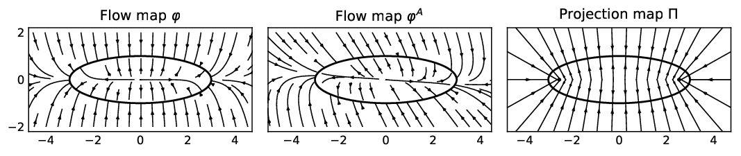
Let us make a comparison among the three schemes (57), (60) and (62). From Figure 1 and Figure 2, we can see that the three maps Θ\Theta, ΘA\Theta^{A} and Π\Pi indeed have different effects. Roughly speaking, comparing to the projection map Π\Pi, both Θ\Theta and ΘA\Theta^{A} tend to map states towards one of the two vertices (±c,0)(\pm c,0), where |∇ξ||\nabla\xi| are smaller, while ΠA\Pi^{A} introduces a further rotational force on Σ\Sigma. Based on the states generated from these three schemes, in Figure 3 we show the empirical probability densities of the parameter θ\theta in (55). From the agreement between the empirical densities and the densities computed from the analytical expressions in (56), we can make the conclusion that the trajectories generated from the two schemes using Θ\Theta and ΘA\Theta^{A} indeed sample the probability measure μ1\mu_{1}, while the trajectory generated from the scheme using Π\Pi samples μ2\mu_{2}.

Lastly, concerning the fourth scheme, we simulate (63) for n=107n=10^{7} steps using the step-size h=0.0001h=0.0001. In this case, we find that it is necessary to choose a small step-size hh in order to keep the trajectory close to the level set Σ\Sigma. As can be seen from Figure 4, even with this smaller step-size h=0.0001h=0.0001, the generated trajectory departs from the level set Σ\Sigma. This indicates the limited usefulness of the direct Euler-Maruyama discretization of the SDE (21) in long time simulations.

Refer to caption
Figure 1: Example 11. Given x∈ℝ2x\in\mathbb{R}^{2}, Π⁡(x)\Pi(x) is the state on the ellipse Σ\Sigma which achieves the minimal distance to xx, while Θ⁡(x)\Theta(x) and ΘA​(x)\Theta^{A}(x) are the limits of the ODE flows (58) and (61) starting from xx, respectively.
Refer to caption
Figure 2: Example 11. Left: the streamline of the flow map φ\varphi in (58). Middle: the streamline of the flow map φA\varphi^{A} (61) with the matrix AA in (59). Right: illustration of the projection Π\Pi. Points on each straight line are mapped to the same point on Σ\Sigma.
Refer to caption
Figure 3: Example 11. The probability densities of the parameter θ\theta, computed from the scheme (57) using Θ\Theta (left plot), the scheme (60) using ΘA\Theta^{A} (middle plot), and the scheme (62) using Π\Pi (right plot). In each plot, dotted curves are the probability densities computed from the analytical expressions of μ1,μ2\mu_{1},\mu_{2} in (56), respectively. Solid lines are the empirical probability densities of θ\theta estimated using the states generated from the schemes (57), (60) and (62), respectively.
Refer to caption
Figure 4: Example 11. States generated from the Euler-Maruyama discretization (63), where we choose h=0.0001h=0.0001 and n=107n=10^{7}. In this case, the sampled states deviate from the level set Σ\Sigma.

Example 2: Numerical comparison with the Metropolis-adjusted method on the special orthogonal group S​O​(11)SO(11).

In this example, we compare the computational efficiency between our scheme (40) using the flow map Θ\Theta and the Metropolis-adjusted method introduced in [43]. We consider the special orthogonal group S​O​(11)SO(11), which consists of orthogonal matrices of size 11×1111\times 11 with determinant equals to 11. This example is taken from [43]. The authors there applied their method to the estimation of the mean value of the function f​(x)=Tr​(x)f(x)=\mbox{Tr}(x), i.e, the trace of the matrix xx, where xx follows the surface measure of S​O​(11)SO(11). The manifold S​O​(11)SO(11) can be viewed as (one connected component of) the level set of the map ξ:ℝ121→ℝ66\xi:\mathbb{R}^{121}\rightarrow\mathbb{R}^{66}, which includes all the row ortho-normality constraints. Readers are referred to the original work [43] for a detailed introduction on the example.

In this numerical study, we implement both the scheme (40) and the (Metropolis-adjusted) algorithm in [43] to estimate the mean value of Tr​(x)\mbox{Tr}(x). Notice that, since det(∇ξT∇ξ)\det(\nabla\xi^{T}\nabla\xi) is constant, the conditional measure μ1\mu_{1} in (2) coincides with the surface measure of S​O​(11)SO(11) when we choose the potential U≡0U\equiv 0. In both cases, we generate n=106n=10^{6} samples on the same laptop (CPU: Intel Core i5, 2.602.60GHz, 44 cores; system: Ubuntu 18.0418.04). For the scheme (40), we choose the step-size h=0.022h=0.022. The map Θ\Theta is computed by integrating the ODE (36) with a=ida=\mbox{id}, until the condition |ξ⁡(φ⁡(x,s))|<10−9|\xi(\varphi(x,s))|<10^{-9} is satisfied. To accelerate the ODE integration, we have applied the adaptivity technique in the second point of Remark 5 with κ=0.5\kappa=0.5. Starting from the initial step-size Δ​s=0.2\Delta s=0.2, the step-size used in the ODE integration is divided by 2.02.0 whenever we find that the value of |ξ||\xi| is not decreasing. (The numerical error of Θ\Theta is 2.0×10−42.0\times 10^{-4} on average, comparing to the reference solution that is obtained by solving the ODE with κ=0\kappa=0 and the fixed step-size Δ​s=0.002\Delta s=0.002.) Furthermore, the new state will be discarded (and resampled) if its determinant equals to −1-1. With these parameters, we observe that on average 3737 Runge-Kutta iterations are needed for each evaluation of the map Θ\Theta. In total, it takes 2676.92676.9 seconds to generate n=106n=10^{6} samples, while the estimated mean value of Tr​(x)\mbox{Tr}(x) is 3.8×10−33.8\times 10^{-3} with a statistical error 3.9×10−33.9\times 10^{-3}. For the algorithm in [43], the maximal number of Newton steps is set to 1010 and the proposal length scale is chosen to be 0.2570.257 11 1 The roles of the proposal length scale in [43] and the step-size hh in the scheme (40) are different. The proposal length scale 0.2570.257 used in this example corresponds to a step-size 0.0330.033 (≈0.2572/2\approx 0.257^{2}/2) in the scheme (40).. In our experiment, we find that this proposal length scale (different from the one used in [43]) leads to slightly smaller correlation time. Within the entire computation, the success rate of the Newton’s method (i.e., the rate that the Newton’s method converges) is 67.2%67.2\% and each time it takes 55-66 iterations on average for the Newton’s method to reach convergence (the convergence criteria is |ξ⁡(x)|<10−9|\xi(x)|<10^{-9}). In total, it takes 7315.97315.9 seconds to generate n=106n=10^{6} samples. The estimated mean value is −3.8×10⁻³-3.8\times 10^{-3} and the statistical error is 3.8×10−33.8\times 10^{-3}.

The empirical density distributions of Tr​(x)\mbox{Tr}(x) using both the scheme (40) and the algorithm in [43] are shown in the left plot of Figure 5, while the autocorrelation functions are plotted in the right plot of Figure 5. From these results, we can conclude that in this example both approaches provide similar statistical estimations (The autocorrelation time using Metropolis-adjusted method is slightly smaller with the above parameters.). At the same time, the total computational time using the scheme (40) is less than half of the computational time required by the algorithm in [43]. For this example, although the average number of Newton steps in the latter algorithm is smaller than the average number of ODE iterations, the computational cost of each Newton step is indeed larger. We refer to Remark 8 for the comparison of computational complexity of both approaches.

Refer to caption
Refer to caption
Figure 5: Example 22. Left: empirical density plots of the statistics Tr​(x)\mbox{Tr}(x), where x∈S​O​(11)x\in SO(11). Both empirical densities resemble the probability density of the standard Gaussian random variable. Right: autocorrelation functions of the sampled trajectories. In both plots, the curve with label “projection by Θ\Theta” and the curve with label “MCMC” are the results obtained using the scheme (40) and the Metropolis-adjusted algorithm in [43], respectively.

Example 3: Removing stiffness by choosing a non-constant matrix aa

In this example, we choose the reaction coordinate function

ξ⁡(x)=ξ⁡(x1,x2,⋯,xd)=12​(x12+x22+⋯+xd2−1).\displaystyle\xi(x)=\xi(x_{1},x_{2},\cdots,x_{d})=\frac{1}{2}\Big(x_{1}^{2}+x_{2}^{2}+\cdots+x^{2}_{d}-1\Big)\,.

Correspondingly, the level set

Σ={(x1,x2,⋯,xd)∈ℝd|x12+x22+⋯+xd2=1}\displaystyle\Sigma=\Big\{(x_{1},x_{2},\cdots,x_{d})\in\mathbb{R}^{d}~\Big|~x_{1}^{2}+x_{2}^{2}+\cdots+x_{d}^{2}=1\Big\}

is the (d−1)(d-1)-dimensional unit sphere, and we have

∇ξ=(x1,x2,⋯,xd)T,∇ξT∇ξ=∑i=1dxi2.\displaystyle\nabla\xi=(x_{1},x_{2},\cdots,x_{d})^{T},\quad\nabla\xi^{T}\nabla\xi=\sum_{i=1}^{d}x_{i}^{2}\,.

In the following, we give an example to show that in some applications it is helpful to use a non-constant matrix aa in the numerical scheme (40). Briefly speaking, varying the matrix aa properly allows to rescale the scheme along different directions. It has a preconditioning effect when different time scales (stiffness) exist.

Consider d=3d=3 and the potential U=θ22​ϵU=\frac{\theta^{2}}{2\epsilon}, where ϵ>0\epsilon>0 is a small parameter, θ\theta is the angle of the state x=(x1,x2,x3)x=(x_{1},x_{2},x_{3}) under the spherical coordinate system

x1=ρ​cos⁡θ​cos⁡φ,x2=ρ​cos⁡θ​sin⁡φ,x3=ρ​sin⁡θ,\displaystyle x_{1}=\rho\cos\theta\cos\varphi\,,\quad x_{2}=\rho\cos\theta\sin\varphi\,,\quad x_{3}=\rho\sin\theta\,,

where ρ≥0\rho\geq 0, θ∈[−π2,π2]\theta\in[-\frac{\pi}{2},\frac{\pi}{2}], and φ∈[0,2​π]\varphi\in[0,2\pi]. We can verify that

∇θ=1ρ2​(−x1​x3(x12+x22)12,−x2​x3(x12+x22)12,(x12+x22)12)T.\displaystyle\nabla\theta=\frac{1}{\rho^{2}}\Big(-\frac{x_{1}x_{3}}{(x_{1}^{2}+x_{2}^{2})^{\frac{1}{2}}},\,-\frac{x_{2}x_{3}}{(x_{1}^{2}+x_{2}^{2})^{\frac{1}{2}}},\,(x_{1}^{2}+x_{2}^{2})^{\frac{1}{2}}\Big)^{T}\,. (65)

Correspondingly, with the choice of σ=a=id\sigma=a=\mbox{id}, the scheme (40) is

x(l+12)=x(l)−1ϵ(θ∇θ)(x(l))h+2​β−1​h𝜼(l),x(l+1)=Θ⁡(x(l+12)),\displaystyle\begin{split}x^{(l+\frac{1}{2})}=&x^{(l)}-\frac{1}{\epsilon}(\theta\nabla\theta)(x^{(l)})\,h+\sqrt{2\beta^{-1}h}\,\bm{\eta}^{(l)}\,,\\ x^{(l+1)}=&\Theta\big(x^{(l+\frac{1}{2})}\big)\,,\end{split} (66)

where ∇θ\nabla\theta is given in (65). Notice that, the coefficients in (66) are 𝒪⁡(1ϵ)\mathcal{O}(\frac{1}{\epsilon}) when ϵ\epsilon is small. In particular, it implies that sampling the invariant measure using (66) will be inefficient when ϵ\epsilon is small, since the step-size hh will be severely limited due to the large magnitude of the coefficients in (66).

On the other hand, based on the form of UU and the expression (65), we consider the orthogonal vectors

𝝈1=(x1,x2,x3)T=∇ξ,𝝈2=(x2,−x1,0)T,𝝈3=(−ϵ​x1​x3(x12+x22)12,−ϵ​x2​x3(x12+x22)12,ϵ(x12+x22)12)T=ϵρ2∇θ,\displaystyle\begin{split}\bm{\sigma}_{1}=&(x_{1},x_{2},x_{3})^{T}=\nabla\xi\,,\quad\bm{\sigma}_{2}=(x_{2},-x_{1},0)^{T}\,,\\ \bm{\sigma}_{3}=&\Big(-\frac{\sqrt{\epsilon}\,x_{1}x_{3}}{(x_{1}^{2}+x_{2}^{2})^{\frac{1}{2}}},-\frac{\sqrt{\epsilon}\,x_{2}x_{3}}{(x_{1}^{2}+x_{2}^{2})^{\frac{1}{2}}},\sqrt{\epsilon}(x_{1}^{2}+x_{2}^{2})^{\frac{1}{2}}\Big)^{T}=\sqrt{\epsilon}\rho^{2}\nabla\theta\,,\end{split}

and we define σ=(𝝈1,𝝈2,𝝈3)∈ℝ3×3\sigma=(\bm{\sigma}_{1},\bm{\sigma}_{2},\bm{\sigma}_{3})\in\mathbb{R}^{3\times 3}. Direct calculation shows that

a=σ​σT=(x12+x22+ϵ​x12​x32x12+x22ϵ​x1​x2​x32x12+x22(1−ϵ)​x1​x3ϵ​x1​x2​x32x12+x22x12+x22+ϵ​x22​x32x12+x22(1−ϵ)​x2​x3(1−ϵ)​x1​x3(1−ϵ)​x2​x3x32+ϵ⁡(x12+x22)).\displaystyle a=\sigma\sigma^{T}=\begin{pmatrix}x_{1}^{2}+x_{2}^{2}+\frac{\epsilon x_{1}^{2}x_{3}^{2}}{x_{1}^{2}+x_{2}^{2}}&\frac{\epsilon x_{1}x_{2}x_{3}^{2}}{x_{1}^{2}+x_{2}^{2}}&(1-\epsilon)x_{1}x_{3}\\ \frac{\epsilon x_{1}x_{2}x_{3}^{2}}{x_{1}^{2}+x_{2}^{2}}&x_{1}^{2}+x_{2}^{2}+\frac{\epsilon x_{2}^{2}x_{3}^{2}}{x_{1}^{2}+x_{2}^{2}}&(1-\epsilon)x_{2}x_{3}\\ (1-\epsilon)x_{1}x_{3}&(1-\epsilon)x_{2}x_{3}&x_{3}^{2}+\epsilon(x_{1}^{2}+x_{2}^{2})\end{pmatrix}\,. (67)

Correspondingly, using (67), the scheme (40) becomes

xi(l+12)=xi(l)+[−θ​∂θ∂xi+1β​∂ai​j∂xj]​(x(l))​h+2​β−1​h​σi​j​(x(l))​𝜼j(l),1≤i≤3,x(l+1)=Θ⁡(x(l+12)),\displaystyle\begin{split}x^{(l+\frac{1}{2})}_{i}=&x^{(l)}_{i}+\Big[-\theta\frac{\partial\theta}{\partial x_{i}}+\frac{1}{\beta}\frac{\partial a_{ij}}{\partial x_{j}}\Big](x^{(l)})\,h+\sqrt{2\beta^{-1}h}\,\sigma_{ij}(x^{(l)})\,\bm{\eta}^{(l)}_{j}\,,\quad 1\leq i\leq 3\,,\\ x^{(l+1)}=&\Theta\big(x^{(l+\frac{1}{2})}\big)\,,\end{split} (68)

where Θ⁡(x)\Theta(x) is the limit of the ODE flow

y˙​(s)=−ξ⁡(y⁡(s))​(2​ξ​(y⁡(s))+1)​y​(s),y⁡(0)=x.\displaystyle\dot{y}(s)=-\xi\big(y(s)\big)\Big(2\xi\big(y(s)\big)+1\Big)\,y(s)\,,\quad y(0)=x\,. (69)

Importantly, in contrast to (66), the scheme (68)–(69) is no longer stiff when ϵ\epsilon is small.

Now we compare the numerical efficiency between the schemes (66) and (68)–(69). First of all, since the surface measure on Σ\Sigma satisfies d​ν=cos⁡θ​d​θ​d​φd\nu=\cos\theta d\theta\,d\varphi, we know that the target measure is

d​μ=1Z​e−β​θ22​ϵ​d​ν=1Z​e−β​θ22​ϵ​cos⁡θ​d​θ​d​φ.\displaystyle d\mu=\frac{1}{Z}e^{-\frac{\beta\theta^{2}}{2\epsilon}}d\nu=\frac{1}{Z}e^{-\frac{\beta\theta^{2}}{2\epsilon}}\cos\theta\,d\theta\,d\varphi\,. (70)

In the numerical study, we choose ϵ=0.005\epsilon=0.005 and generate n=107n=10^{7} states for both schemes. For the scheme (66) which corresponds to a=ida=\mbox{id}, we use both a small step-size h=0.0002h=0.0002 and a (relatively) larger step-size h=0.005h=0.005, while we choose a large step-size h=0.01h=0.01 in the scheme (68)–(69) . The empirical probability densities of the angles θ,φ\theta,\varphi for the two schemes are shown in Figure 6 and Figure 7, respectively. From Figure 6, we see that the step-size hh has to be small (h=0.0002h=0.0002) in (66) in order to produce the correct probability density of the angle θ\theta (left plot). However, with such a small hh, the estimated empirical density of the angle φ\varphi (right plot) is still noisy with n=107n=10^{7}. On the other hand, for the scheme (68)–(69) which corresponds to the matrix aa in (67), Figure 7 shows that the probability densities of both angles θ,φ\theta,\varphi are well approximated using the large step-size h=0.01h=0.01. Therefore, we conclude that in this example choosing the non-constant matrix aa in (67) indeed helps improve the sampling efficiency.

Refer to caption
Figure 6: Example 33. The empirical densities of the angles θ\theta and φ\varphi are estimated using the scheme (66) which corresponds to a=ida=\mbox{id}. ϵ=0.005\epsilon=0.005 and n=107n=10^{7} states are sampled, using a small step-size h=0.0002h=0.0002 and a larger step-size h=0.005h=0.005. The curves with label “exact” are the analytical marginal densities computed from (70).
Refer to caption
Figure 7: Example 33. The empirical densities of the angles θ\theta and φ\varphi are estimated using the scheme (68)–(69) which corresponds to the matrix aa in (67). ϵ=0.005\epsilon=0.005 and n=107n=10^{7} states are sampled using a large step-size h=0.01h=0.01. The curves with label “exact” are the analytical marginal densities computed from (70).

5 Conclusions

Ergodic diffusion processes on a submanifold of ℝd\mathbb{R}^{d} and related numerical sampling schemes have been considered in this work. A family of SDEs has been obtained whose invariant measures coincide with the given probability measure on the submanifold. In particular, for the conditional probability measure, we found that the corresponding SDEs have a relatively simple form. We proposed and analyzed a consistent numerical scheme which only requires 11st order derivatives of the reaction coordinate function. Different sampling schemes on the submanifolds are numerically evaluated.

The current work extends results in the literature and may further contribute to both the analysis and the development of numerical methods on related problems, in particular problems in molecular dynamics such as free energy calculation and model reduction of high-dimensional stochastic processes. Closely related to the current paper, the following topics could be considered. First, the “non-reversible” scheme (49) is supported by a simple numerical example but theoretical justification still needs to be investigated. This will be considered in future following the approach described in Remark 7. Second, the constrained numerical schemes in the current work do not involve system’s momentum variables. In view of the work [32], it is interesting to study the Langevin dynamics under different constraints (such as certain variants of the map Θ\Theta used in this work). Third, there is a research interest in the literature to study the effective dynamics of molecular systems along a given reaction coordinate ξ\xi. The coefficients of the effective dynamics are usually defined as averages on the level set of ξ\xi [27]. As an application of the numerical scheme proposed in this work, we will study numerical algorithms to simulate the effective dynamics. This topic is related to the heterogeneous multiscale methods [13] and the equation-free approach [26, 24] in the literature.

Acknowledgement

This work is funded by the Einstein Center of Mathematics (ECMath) through project CH21. The author would like to thank Gabriel Stoltz for stimulating discussions on constrained Langevin processes at the Institut Henri Poincaré - Centre Émile Borel during the trimester “Stochastic Dynamics Out of Equilibrium”. The author appreciates the hospitality of this institution. The author also thanks the anonymous referees for their valuable comments and criticism which helped improve the manuscript substantially.

Appendix A Useful facts about the Riemannian manifold ℳ\mathcal{M}

In this section, we present technical details of Section 2 related to the Riemannian manifold ℳ=(ℝd,g)\mathcal{M}=(\mathbb{R}^{d},g), where g=a−1g=a^{-1}. The main result is Proposition 5, where we give the expression of the Laplacian-Beltrami operator ΔΣ\Delta^{\Sigma} on the level set Σ\Sigma in (1), viewed as a submanifold of ℳ\mathcal{M}. Before that, we first introduce some notations and quantities related to ℳ\mathcal{M} and Σ\Sigma. Readers are referred to [12, 6, 22, 39] for related discussions on general Riemannian manifolds.

Under Assumption 1, given two vectors 𝒖=(u1,u2,⋯,ud)T\bm{u}=(u_{1},u_{2},\cdots,u_{d})^{T}, 𝒗=(v1,v2,⋯,vd)T\bm{v}=(v_{1},v_{2},\cdots,v_{d})^{T}, we consider the space ℝd\mathbb{R}^{d} with the weighted inner product

g⁡(𝒖,𝒗)=⟨𝒖,𝒗⟩g=ui​(a−1)i​j​vj.\displaystyle g(\bm{u},\bm{v})=\langle\bm{u},\bm{v}\rangle_{g}=u_{i}(a^{-1})_{ij}v_{j}\,. (71)

The inner product in (71) defines a Riemannian metric gg on ℝd\mathbb{R}^{d} and we denote by ℳ=(ℝd,g)\mathcal{M}=(\mathbb{R}^{d},g) the Riemannian manifold ℝd\mathbb{R}^{d} endowed with this metric.

Notice that ℳ\mathcal{M} as a manifold is quite special (simple), in that it has a natural global coordinate chart which is given by the usual Euclidean coordinate. Since we will always work with this coordinate, we will not distinguish between tangent vectors (operators acting on functions) and their coordinate representations (dd-dimensional vectors). In particular, 𝒆i\bm{e}_{i} denotes the vector whose iith component equals to 11 while all the other d−1d-1 components equal to 00, where 1≤i≤d1\leq i\leq d. At each point x∈ℳx\in\mathcal{M}, vectors 𝒆1,𝒆2,⋯,𝒆d\bm{e}_{1},\bm{e}_{2},\,\cdots,\bm{e}_{d} form a basis of the tangent space Tx​ℳT_{x}\mathcal{M} and under this basis we have g=a−1g=a^{-1}, as can be seen from (71).

Denote by gradℳ\mbox{grad}^{\mathcal{M}}, divℳ\mbox{div}^{\mathcal{M}} the gradient and the divergence operator on ℳ\mathcal{M}, respectively. For any smooth function f:ℳ→ℝf:\mathcal{M}\rightarrow\mathbb{R}, it is direct to verify that

gradℳf=gi​j∂f∂xj𝒆i=(a∇f)i𝒆i,\displaystyle\mbox{grad}^{\mathcal{M}}f=g^{ij}\frac{\partial f}{\partial x_{j}}\bm{e}_{i}=(a\nabla f)_{i}\,\bm{e}_{i}\,,

where gi​j=(g−1)i​j=ai​jg^{ij}=(g^{-1})_{ij}=a_{ij}, and ∇f\nabla f denotes the ordinary gradient operator for functions on the Euclidean space ℝd\mathbb{R}^{d}. For simplicity, we will also write ∂if\partial_{i}f for the partial derivative with respect to xix_{i}, and (a∇f)i(a\nabla f)_{i} to denote the iith component of the vector a∇fa\nabla f, i.e., ∂if=∂f∂xi\partial_{i}f=\frac{\partial f}{\partial x_{i}}, and (a∇f)i=ai​j∂f∂xj=ai​j∂jf(a\nabla f)_{i}=a_{ij}\frac{\partial f}{\partial x_{j}}=a_{ij}\partial_{j}f.

The Laplace-Beltrami operator on ℳ\mathcal{M} is defined by Δℳ​f=divℳ​(gradℳ​f)\Delta^{\mathcal{M}}f=\mbox{div}^{\mathcal{M}}(\mbox{grad}^{\mathcal{M}}f). Equivalently, we have Δℳ​f=tr​(Hessℳ​f)\Delta^{\mathcal{M}}f=\mbox{tr}(\mbox{Hess}^{\mathcal{M}}f), where Hessℳ\mbox{Hess}^{\mathcal{M}} is the Hessian operator on ℳ\mathcal{M}. The integration by parts formula on ℳ\mathcal{M} has the form

∫ℳ(Δℳf1)f2dm=−∫ℳ⟨gradℳf1,gradℳf2⟩gdm=∫ℳ(Δℳf2)f1dm,\displaystyle\int_{\mathcal{M}}(\Delta^{\mathcal{M}}f_{1})\,f_{2}\,dm=-\int_{\mathcal{M}}\langle\mbox{grad}^{\mathcal{M}}f_{1},\mbox{grad}^{\mathcal{M}}f_{2}\rangle_{g}\,dm=\int_{\mathcal{M}}(\Delta^{\mathcal{M}}f_{2})f_{1}\,dm\,, (72)

for ∀f1,f2∈C0∞​(ℳ)\forall f_{1},\,f_{2}\in C^{\infty}_{0}(\mathcal{M}), where d​m=(detg)12​d​x=(deta)−12​d​xdm=(\det g)^{\frac{1}{2}}dx=(\det a)^{-\frac{1}{2}}dx is the volume form, and C0∞​(ℳ)C^{\infty}_{0}(\mathcal{M}) consists of all smooth functions on ℳ\mathcal{M} with compact support.

Besides the vector basis 𝒆1,𝒆2,⋯,𝒆d\bm{e}_{1},\,\bm{e}_{2},\,\cdots,\bm{e}_{d}, the vectors

𝝈i=(σ1​i,σ2​i,⋯,σd​i)T,1≤i≤d,\displaystyle\bm{\sigma}_{i}=(\sigma_{1i},\sigma_{2i},\cdots,\sigma_{di})^{T},\quad 1\leq i\leq d\,, (73)

will also be useful. Note that a=σ​σT=g−1a=\sigma\sigma^{T}=g^{-1} implies ⟨𝝈i,𝝈j⟩g=(a−1)r​l​σr​i​σl​j=δi​j\langle\bm{\sigma}_{i},\bm{\sigma}_{j}\rangle_{g}=(a^{-1})_{rl}\sigma_{ri}\sigma_{lj}=\delta_{ij}. In other words, 𝝈1,𝝈2,⋯,𝝈d\bm{\sigma}_{1},\,\bm{\sigma}_{2},\,\cdots,\bm{\sigma}_{d} form an orthonormal basis of Tx​ℳT_{x}\mathcal{M} at each x∈ℳx\in\mathcal{M}.

Denote by ∇ℳ\nabla^{\mathcal{M}} the Levi-Civita connection on ℳ\mathcal{M}. Given x∈ℳx\in\mathcal{M} and a tangent vector 𝒗∈Tx​ℳ\bm{v}\in T_{x}\mathcal{M}, ∇𝒗ℳ\nabla^{\mathcal{M}}_{\bm{v}} is the covariant derivative operator on ℳ\mathcal{M} along the vector 𝒗\bm{v}. For two vectors 𝒖=(u1,u2,⋯,ud)T\bm{u}=(u_{1},u_{2},\cdots,u_{d})^{T}, 𝒗=(v1,v2,⋯,vd)T\bm{v}=(v_{1},v_{2},\cdots,v_{d})^{T}, the Hessian of a smooth function f:ℳ→ℝf:\mathcal{M}\rightarrow\mathbb{R} is defined as

Hessℳ​f​(𝒖,𝒗)=𝒖⁡(𝒗​f)−(∇𝒖ℳ𝒗)​f=ui​vj​Hessℳ​f​(𝒆i,𝒆j)=ui​vj​(∂2f∂xi​∂xj−Γi​jl​∂f∂xl),\displaystyle\mbox{Hess}^{\mathcal{M}}f(\bm{u},\bm{v})=\bm{u}(\bm{v}f)-(\nabla^{\mathcal{M}}_{\bm{u}}\bm{v})f=u_{i}v_{j}\mbox{Hess}^{\mathcal{M}}f\big(\bm{e}_{i},\bm{e}_{j}\big)=u_{i}v_{j}\Big(\frac{\partial^{2}f}{\partial x_{i}\partial x_{j}}-\Gamma_{ij}^{l}\frac{\partial f}{\partial x_{l}}\Big)\,, (74)

where

Γi​jl=\displaystyle\Gamma_{ij}^{l}= 12gl​r(∂gi​r∂xj+∂gj​r∂xi−∂gi​j∂xr)=12al​r(∂(a−1)i​r∂xj+∂(a−1)j​r∂xi−∂(a−1)i​j∂xr),1≤i,j,l≤d\displaystyle\frac{1}{2}g^{lr}\Big(\frac{\partial g_{ir}}{\partial x_{j}}+\frac{\partial g_{jr}}{\partial x_{i}}-\frac{\partial g_{ij}}{\partial x_{r}}\Big)=\frac{1}{2}a_{lr}\Big(\frac{\partial(a^{-1})_{ir}}{\partial x_{j}}+\frac{\partial(a^{-1})_{jr}}{\partial x_{i}}-\frac{\partial(a^{-1})_{ij}}{\partial x_{r}}\Big)\,,\quad 1\leq i,j,l\leq d (75)

are the Christoffel’s symbols defined by ∇𝒆iℳ𝒆j=Γi​jl​𝒆l\nabla^{\mathcal{M}}_{\bm{e}_{i}}\bm{e}_{j}=\Gamma^{l}_{ij}\bm{e}_{l}, for 1≤i,j≤d1\leq i,j\leq d.

Now let us consider the level set

Σ=ξ−1​(𝟎)={x∈ℳ=ℝd|ξ⁡(x)=𝟎∈ℝk}\displaystyle\Sigma=\xi^{-1}(\bm{0})=\Big\{x\in\mathcal{M}=\mathbb{R}^{d}~\Big|~\xi(x)=\bm{0}\in\mathbb{R}^{k}\Big\} (76)

of the C2C^{2} function ξ:ℝd→ℝk\xi:\mathbb{R}^{d}\rightarrow\mathbb{R}^{k} with ξ=(ξ1,ξ2,⋯,ξk)T\xi=(\xi_{1},\xi_{2},\cdots,\xi_{k})^{T}, 1≤k<d1\leq k<d. Applying regular value theorem [5], we know that Σ\Sigma is a (d−k)(d-k)-dimensional submanifold of ℳ\mathcal{M}, under Assumption 2.

Given x∈Σx\in\Sigma and a vector 𝒗∈Tx​ℳ\bm{v}\in T_{x}\mathcal{M}, the orthogonal projection operator (d×dd\times d matrix) P:ℝd→Tx​ΣP:\mathbb{R}^{d}\rightarrow T_{x}\Sigma is defined such that ⟨𝒗−P​𝒗,𝒖⟩g=0\langle\bm{v}-P\bm{v},\bm{u}\rangle_{g}=0, for ∀𝒖∈Tx​Σ\forall\,\bm{u}\in T_{x}\Sigma\,. It is straightforward to verify that P=id−a∇ξΨ−1∇ξTP=\mbox{id}-a\nabla\xi\Psi^{-1}\nabla\xi^{T}, or entry-wise,

Pi​j=δi​j−(Ψ−1)α​γ(a∇ξα)i∂jξγ,1≤i,j≤d,\displaystyle P_{ij}=\delta_{ij}-(\Psi^{-1})_{\alpha\gamma}\,(a\,\nabla\xi_{\alpha})_{i}\partial_{j}\xi_{\gamma}\,,\quad 1\leq i,j\leq d\,, (77)

where Ψ\Psi is the invertible k×kk\times k symmetric matrix at each point x∈Σx\in\Sigma, given by

Ψα​γ=⟨gradℳξα,gradℳξγ⟩g=(∇ξTa∇ξ)α​γ,1≤α,γ≤k.\displaystyle\Psi_{\alpha\gamma}=\langle\mbox{grad}^{\mathcal{M}}\xi_{\alpha},\mbox{grad}^{\mathcal{M}}\xi_{\gamma}\rangle_{g}=(\nabla\xi^{T}a\nabla\xi)_{\alpha\gamma}\,,\quad 1\leq\alpha,\gamma\leq k\,. (78)

In the above, ∇ξ\nabla\xi denotes the d×kd\times k matrix with entries (∇ξ)i​α=∂iξα(\nabla\xi)_{i\alpha}=\partial_{i}\xi_{\alpha}, for 1≤α≤k1\leq\alpha\leq k, 1≤i≤d1\leq i\leq d. We can verify that

aPT=Pa,P2=P,PT∇ξα=0,1≤α≤k.\displaystyle\quad aP^{T}=Pa,\quad P^{2}=P\,,\quad P^{T}\nabla\xi_{\alpha}=0\,,\quad 1\leq\alpha\leq k\,. (79)

Let us further assume that 𝒗∈Tx​Σ\bm{v}\in T_{x}\Sigma is a tangent vector of Σ\Sigma at xx. Since {𝝈i}1≤i≤d\{\bm{\sigma}_{i}\}_{1\leq i\leq d} forms an orthonormal basis of the tangent space Tx​ℳT_{x}\mathcal{M}, we have 𝒗=⟨𝒗,𝝈i⟩g​𝝈i\bm{v}=\langle\bm{v},\bm{\sigma}_{i}\rangle_{g}\bm{\sigma}_{i}. Using the fact that P​𝒗=𝒗P\bm{v}=\bm{v}, we obtain 𝒗=⟨𝒗,𝒑i⟩g​𝒑i\bm{v}=\langle\bm{v},\bm{p}_{i}\rangle_{g}\bm{p}_{i}, where 𝒑i=P​𝝈i∈Tx​Σ\bm{p}_{i}=P\bm{\sigma}_{i}\in T_{x}\Sigma. If we denote 𝒑i=Pi,j​𝒆j\bm{p}_{i}=P_{i,j}\bm{e}_{j}, then it follows from (77) and (79) that

Pi,j=(Pσ)j​i=σj​i−(Ψ−1)α​γ(a∇ξα)j(σT∇ξγ)iPl,iPl,j=(Pa)i​j=(aPT)i​j=ai​j−(Ψ−1)α​γ(a∇ξα)i(a∇ξγ)j,\displaystyle\begin{split}&P_{i,j}=(P\sigma)_{ji}=\sigma_{ji}-(\Psi^{-1})_{\alpha\gamma}(a\nabla\xi_{\alpha})_{j}(\sigma^{T}\nabla\xi_{\gamma})_{i}\\ &P_{l,i}P_{l,j}=(Pa)_{ij}=(aP^{T})_{ij}=a_{ij}-(\Psi^{-1})_{\alpha\gamma}(a\nabla\xi_{\alpha})_{i}(a\nabla\xi_{\gamma})_{j}\,,\end{split} (80)

for 1≤i,j≤d1\leq i,j\leq d.

Let gradΣ\mbox{grad}^{\Sigma}, divΣ\mbox{div}^{\Sigma}, ΔΣ\Delta^{\Sigma}, HessΣ\mbox{Hess}^{\Sigma} denote the gradient operator, the divergence operator, the Laplace-Beltrami operator and the Hessian operator on Σ\Sigma, respectively. It is direct to check that the Levi-Civita connection and the gradient operator on Σ\Sigma are given by ∇Σ=P​∇ℳ\nabla^{\Sigma}=P\nabla^{\mathcal{M}} and gradΣ=P​gradℳ\mbox{grad}^{\Sigma}=P\,\mbox{grad}^{\mathcal{M}}, respectively. In particular, for f∈C∞​(Σ)f\in C^{\infty}(\Sigma) and let f~\widetilde{f} be its extension to ℳ\mathcal{M} such that f~∈C∞​(ℳ)\widetilde{f}\in C^{\infty}(\mathcal{M}) and f~|Σ=f\widetilde{f}|_{\Sigma}=f, we have

gradΣf=Pgradℳf~=Pa∇f~.\displaystyle\mbox{grad}^{\Sigma}f=P\mbox{grad}^{\mathcal{M}}\widetilde{f}=Pa\nabla\widetilde{f}\,.

Let νg\nu_{g} be the surface measure on Σ\Sigma induced from the metric gg on ℳ\mathcal{M}. We recall that the mean curvature vector HH on Σ\Sigma is defined such that [2, 10]

∫ΣdivΣ𝒗dνg=−∫Σ⟨H,𝒗⟩gdνg,\displaystyle\int_{\Sigma}\mbox{div}^{\Sigma}\bm{v}\,d\nu_{g}=-\int_{\Sigma}\langle H,\bm{v}\rangle_{g}\,d\nu_{g}\,, (81)

for all vector fields 𝒗\bm{v} on ℳ\mathcal{M}.

We have the following lemma, concerning the operators on Σ\Sigma.

Lemma 3.

Let f∈C∞​(Σ)f\in C^{\infty}(\Sigma) and f~∈C∞​(ℳ)\widetilde{f}\in C^{\infty}(\mathcal{M}) be its extension to ℳ\mathcal{M}. 𝐮∈Γ⁡(T​ℳ)\bm{u}\in\Gamma(T\mathcal{M}) is a tangent vector field on ℳ\mathcal{M} and we recall the vectors 𝐩i=P​𝛔i\bm{p}_{i}=P\bm{\sigma}_{i}, 1≤i≤d1\leq i\leq d. We have

  1. 1.

    divΣ​𝒖=⟨∇𝒑iℳ𝒖,𝒑i⟩g\mbox{{div}}^{\Sigma}\bm{u}=\langle\nabla^{\mathcal{M}}_{\bm{p}_{i}}\bm{u},\bm{p}_{i}\rangle_{g}.

  2. 2.

    (divΣ​𝒑i)​𝒑i+P​∇𝒑iℳ𝒑i=0(\mbox{{div}}^{\Sigma}\bm{p}_{i})\bm{p}_{i}+P\nabla^{\mathcal{M}}_{\bm{p}_{i}}\bm{p}_{i}=0\,.

  3. 3.

    ΔΣ​f=∑i=1d𝒑i2​f~+(divΣ​𝒑i)​𝒑i​f~=∑i=1d𝒑i2​f~−(P​∇𝒑iℳ𝒑i)​f~\Delta^{\Sigma}f=\sum\limits_{i=1}^{d}\bm{p}_{i}^{2}\widetilde{f}+(\mbox{{div}}^{\Sigma}\bm{p}_{i})\bm{p}_{i}\widetilde{f}=\sum\limits_{i=1}^{d}\bm{p}_{i}^{2}\widetilde{f}-\big(P\nabla^{\mathcal{M}}_{\bm{p}_{i}}\bm{p}_{i}\big)\widetilde{f}.

  4. 4.

    ΔΣ​f=Hessℳ​f~​(𝒑i,𝒑i)+H​f~\Delta^{\Sigma}f=\mbox{{Hess}}^{\mathcal{M}}\widetilde{f}(\bm{p}_{i},\bm{p}_{i})+H\widetilde{f}, where HH is the mean curvature vector of the submanifold Σ\Sigma.

  5. 5.

    In the special case when g=a=idg=a=\mbox{{id}}, we have (divΣ​𝒑i)​𝒑i=P​∇𝒑iℳ𝒑i=0(\mbox{{div}}^{\Sigma}\bm{p}_{i})\bm{p}_{i}=P\nabla^{\mathcal{M}}_{\bm{p}_{i}}\bm{p}_{i}=0, and ΔΣ=∑i=1d𝒑i2\Delta^{\Sigma}=\sum\limits_{i=1}^{d}\bm{p}_{i}^{2}.

Proof.

The first two assertions can be directly verified. Let us prove the last three assertions. Let x∈Σx\in\Sigma and assume that 𝒗i\bm{v}_{i}, 1≤i≤d−k1\leq i\leq d-k, is an orthonormal basis of Tx​ΣT_{x}\Sigma. We have 𝒗i=⟨𝒗i,𝒑j⟩g​𝒑j\bm{v}_{i}=\langle\bm{v}_{i},\bm{p}_{j}\rangle_{g}\bm{p}_{j}. For the third assertion, by definition,

ΔΣ​f=\displaystyle\Delta^{\Sigma}f= divΣ​(gradΣ​f)=divΣ​(P​gradℳ​f~)=divΣ​(⟨gradℳ​f~,𝒑i⟩g​𝒑i)\displaystyle\mbox{div}^{\Sigma}(\mbox{grad}^{\Sigma}f)=\mbox{div}^{\Sigma}\big(P\,\mbox{grad}^{\mathcal{M}}\widetilde{f}\,\big)=\mbox{div}^{\Sigma}\big(\langle\mbox{grad}^{\mathcal{M}}\widetilde{f},\bm{p}_{i}\rangle_{g}\,\bm{p}_{i}\big)
=\displaystyle= divΣ​((𝒑i​f~)​𝒑i)=∑i=1d𝒑i2​f~+(divΣ​𝒑i)​𝒑i​f~=∑i=1d𝒑i2​f~−(P​∇𝒑iℳ𝒑i)​f~,\displaystyle\mbox{div}^{\Sigma}\big((\bm{p}_{i}\widetilde{f}\,)\bm{p}_{i}\big)=\sum_{i=1}^{d}\bm{p}_{i}^{2}\widetilde{f}+(\mbox{div}^{\Sigma}\bm{p}_{i})\bm{p}_{i}\widetilde{f}=\sum_{i=1}^{d}\bm{p}_{i}^{2}\widetilde{f}-\big(P\nabla^{\mathcal{M}}_{\bm{p}_{i}}\bm{p}_{i}\big)\widetilde{f}\,,

where the second assertion has been used in the last equality.

For the fourth assertion, starting from the third assertion, using the definition of Hessℳ\mbox{Hess}^{\mathcal{M}} in (74), and applying Proposition 4 below, we obtain

ΔΣ​f=\displaystyle\Delta^{\Sigma}f= ∑i=1d𝒑i2​f−P​∇𝒑iℳ𝒑i​f\displaystyle\sum_{i=1}^{d}\bm{p}_{i}^{2}f-P\nabla^{\mathcal{M}}_{\bm{p}_{i}}\bm{p}_{i}f
=\displaystyle= Hessℳ​f~​(𝒑i,𝒑i)+[(I−P)​∇𝒑iℳ𝒑i]​f~=Hessℳ​f~​(𝒑i,𝒑i)+H​f~.\displaystyle\mbox{Hess}^{\mathcal{M}}\widetilde{f}(\bm{p}_{i},\bm{p}_{i})+\big[(I-P)\nabla^{\mathcal{M}}_{\bm{p}_{i}}\bm{p}_{i}\big]\widetilde{f}=\mbox{Hess}^{\mathcal{M}}\widetilde{f}(\bm{p}_{i},\bm{p}_{i})+H\widetilde{f}\,.

For the last assertion, when g=idg=\mbox{{id}}, we have Γi​jl≡0\Gamma_{ij}^{l}\equiv 0, for ∀1≤i,j,l≤d\forall 1\leq i,j,l\leq d. Also, it follows from (80) that Pi,j=Pi​j=Pj​iP_{i,j}=P_{ij}=P_{ji} and Pi​l​Pl​j=Pi​jP_{il}P_{lj}=P_{ij}. We obtain

(divΣ​𝒑i)​𝒑i\displaystyle(\mbox{div}^{\Sigma}\bm{p}_{i})\bm{p}_{i}
=\displaystyle= ⟨∇𝒑jℳ𝒑i,𝒑j⟩g​𝒑i\displaystyle\langle\nabla^{\mathcal{M}}_{\bm{p}_{j}}\bm{p}_{i},\bm{p}_{j}\rangle_{g}\,\bm{p}_{i}
=\displaystyle= Pj,l​Pj,j′​Pi,i′​⟨∇𝒆lℳ(Pi,r​𝒆r),𝒆j′⟩g​𝒆i′\displaystyle P_{j,l}P_{j,j^{\prime}}P_{i,i^{\prime}}\langle\nabla^{\mathcal{M}}_{\bm{e}_{l}}\big(P_{i,r}\bm{e}_{r}\big),\bm{e}_{j^{\prime}}\rangle_{g}\,\bm{e}_{i^{\prime}}
=\displaystyle= Pl​r​∂Pi​r∂xl​Pi​i′​𝒆i′\displaystyle P_{lr}\frac{\partial P_{ir}}{\partial x_{l}}P_{ii^{\prime}}\,\bm{e}_{i^{\prime}}
=\displaystyle= [∂Pi​l∂xl​Pi​i′−∂Pl​r∂xl​Pr​i′]​𝒆i′\displaystyle\Big[\frac{\partial P_{il}}{\partial x_{l}}P_{ii^{\prime}}-\frac{\partial P_{lr}}{\partial x_{l}}P_{ri^{\prime}}\Big]\,\bm{e}_{i^{\prime}}
=\displaystyle= 0,\displaystyle 0\,,

and the other assertions follow accordingly. ∎

Proposition 4.

Let HH be the mean curvature vector defined in (81) on the submanifold Σ\Sigma. We have

H=(I−P)​∇𝒑iℳ𝒑i=−(Ψ−1)α​γ[12(Pa)i​j(a∇ξα)l∂(a−1)i​j∂xl+Pi​l∂(a∇ξα)l∂xi]a∇ξγ.\displaystyle\begin{split}H=&(I-P)\nabla^{\mathcal{M}}_{\bm{p}_{i}}\bm{p}_{i}\\ =&-(\Psi^{-1})_{\alpha\gamma}\bigg[\frac{1}{2}(Pa)_{ij}(a\nabla\xi_{\alpha})_{l}\frac{\partial(a^{-1})_{ij}}{\partial x_{l}}+P_{il}\frac{\partial(a\nabla\xi_{\alpha})_{l}}{\partial x_{i}}\bigg]a\nabla\xi_{\gamma}\,.\end{split} (82)

In the special case when g=a=idg=a=\mbox{{id}}, we have

H=Pj​l∂Pi​l∂xj𝒆i=−[(Ψ−1)α​γPi​j∂i​j2ξα]∇ξγ.\displaystyle H=P_{jl}\frac{\partial P_{il}}{\partial x_{j}}\bm{e}_{i}=-\big[(\Psi^{-1})_{\alpha\gamma}P_{ij}\,\partial^{2}_{ij}\xi_{\alpha}\big]\nabla\xi_{\gamma}\,. (83)
Proof.

Given a tangent vector field 𝒗\bm{v} on ℳ\mathcal{M}, from the definition of PP we have 𝒗=P𝒗+(Ψ−1)α​γ⟨𝒗,a∇ξγ⟩ga∇ξα\bm{v}=P\bm{v}+(\Psi^{-1})_{\alpha\gamma}\langle\bm{v},a\nabla\xi_{\gamma}\rangle_{g}\,a\nabla\xi_{\alpha}. Since P​𝒗P\bm{v} is a tangent vector field on Σ\Sigma, using (81) and the divergence theorem on Σ\Sigma, we know

∫Σ⟨H,𝒗⟩gdνg=−∫ΣdivΣ[(I−P)𝒗]dνg=−∫ΣdivΣ[(Ψ−1)α​γ⟨𝒗,a∇ξγ⟩ga∇ξα]dνg.\displaystyle\int_{\Sigma}\langle H,\bm{v}\rangle_{g}\,d\nu_{g}=-\int_{\Sigma}\mbox{div}^{\Sigma}\big[(I-P)\bm{v}\big]\,d\nu_{g}=-\int_{\Sigma}\mbox{div}^{\Sigma}\big[(\Psi^{-1})_{\alpha\gamma}\langle\bm{v},a\nabla\xi_{\gamma}\rangle_{g}\,a\nabla\xi_{\alpha}\big]\,d\nu_{g}\,. (84)

For the first expression, we notice that ⟨(I−P)​𝒗,𝒑i⟩g≡0\langle(I-P)\bm{v},\bm{p}_{i}\rangle_{g}\equiv 0, 1≤i≤d1\leq i\leq d. Applying Lemma 3, we have

−∫ΣdivΣ[(I−P)𝒗]dνg\displaystyle-\int_{\Sigma}\mbox{div}^{\Sigma}\big[(I-P)\bm{v}\big]d\nu_{g}
=\displaystyle= −∫Σ⟨∇𝒑iℳ[(I−P)𝒗],𝒑i⟩gdνg\displaystyle-\int_{\Sigma}\langle\nabla^{\mathcal{M}}_{\bm{p}_{i}}\big[(I-P)\bm{v}\big],\bm{p}_{i}\rangle_{g}\,d\nu_{g}
=\displaystyle= −∫Σ𝒑i⟨(I−P)𝒗,𝒑i⟩gdνg+∫Σ⟨(I−P)𝒗,∇𝒑iℳ𝒑i⟩gdνg\displaystyle-\int_{\Sigma}\bm{p}_{i}\langle(I-P)\bm{v},\bm{p}_{i}\rangle_{g}\,d\nu_{g}+\int_{\Sigma}\langle(I-P)\bm{v},\nabla^{\mathcal{M}}_{\bm{p}_{i}}\bm{p}_{i}\rangle_{g}\,d\nu_{g}
=\displaystyle= ∫Σ⟨𝒗,(I−P)​∇𝒑iℳ𝒑i⟩g​d​νg.\displaystyle\int_{\Sigma}\langle\bm{v},(I-P)\nabla^{\mathcal{M}}_{\bm{p}_{i}}\bm{p}_{i}\rangle_{g}\,d\nu_{g}\,.

Comparing the last equality above with (84), we conclude that H=(I−P)​∇𝒑iℳ𝒑iH=(I-P)\nabla^{\mathcal{M}}_{\bm{p}_{i}}\bm{p}_{i}.

For the second expression, we notice that ⟨a∇ξα,𝒑i⟩g=0\langle a\nabla\xi_{\alpha},\bm{p}_{i}\rangle_{g}=0, and also recall the expressions (75), (78) and (80). Applying Lemma 3, integrating by parts, and noticing the cancellation of some terms, we can derive

divΣ[(Ψ−1)α​γ⟨𝒗,a∇ξγ⟩ga∇ξα]\displaystyle\mbox{div}^{\Sigma}\big[(\Psi^{-1})_{\alpha\gamma}\langle\bm{v},a\nabla\xi_{\gamma}\rangle_{g}\,a\nabla\xi_{\alpha}\big]
=\displaystyle= ⟨∇𝒑iℳ[(Ψ−1)α​γ⟨𝒗,a∇ξγ⟩ga∇ξα],𝒑i⟩g\displaystyle\langle\nabla^{\mathcal{M}}_{\bm{p}_{i}}\big[(\Psi^{-1})_{\alpha\gamma}\langle\bm{v},a\nabla\xi_{\gamma}\rangle_{g}\,a\nabla\xi_{\alpha}\big],\bm{p}_{i}\rangle_{g}\,
=\displaystyle= (Ψ−1)α​γ⟨𝒗,a∇ξγ⟩g⟨∇𝒑iℳ(a∇ξα),𝒑i⟩g\displaystyle(\Psi^{-1})_{\alpha\gamma}\langle\bm{v},a\nabla\xi_{\gamma}\rangle_{g}\,\langle\nabla^{\mathcal{M}}_{\bm{p}_{i}}(a\nabla\xi_{\alpha}),\bm{p}_{i}\rangle_{g}\,
=\displaystyle= (Ψ−1)α​γ⟨𝒗,a∇ξγ⟩gPi,jPi,l⟨∇𝒆jℳ((a∇ξα)r𝒆r),𝒆l⟩g\displaystyle(\Psi^{-1})_{\alpha\gamma}\langle\bm{v},a\nabla\xi_{\gamma}\rangle_{g}\,P_{i,j}P_{i,l}\langle\nabla^{\mathcal{M}}_{\bm{e}_{j}}\big((a\nabla\xi_{\alpha})_{r}\bm{e}_{r}\big),\bm{e}_{l}\rangle_{g}\,
=\displaystyle= (Ψ−1)α​γ⟨𝒗,a∇ξγ⟩g(Pa)j​l[(a∇ξα)rΓj​ri(a−1)i​l+∂(a∇ξα)r∂xj(a−1)l​r]\displaystyle(\Psi^{-1})_{\alpha\gamma}\langle\bm{v},a\nabla\xi_{\gamma}\rangle_{g}\,(Pa)_{jl}\Big[(a\nabla\xi_{\alpha})_{r}\Gamma^{i}_{jr}(a^{-1})_{il}+\frac{\partial(a\nabla\xi_{\alpha})_{r}}{\partial x_{j}}(a^{-1})_{lr}\Big]
=\displaystyle= (Ψ−1)α​γ⟨𝒗,a∇ξγ⟩g(Pa)i​j[12(a∇ξα)l∂(a−1)i​j∂xl+∂(a∇ξα)l∂xi(a−1)l​j].\displaystyle(\Psi^{-1})_{\alpha\gamma}\langle\bm{v},a\nabla\xi_{\gamma}\rangle_{g}\,(Pa)_{ij}\Big[\frac{1}{2}(a\nabla\xi_{\alpha})_{l}\frac{\partial(a^{-1})_{ij}}{\partial x_{l}}+\frac{\partial(a\nabla\xi_{\alpha})_{l}}{\partial x_{i}}(a^{-1})_{lj}\Big]\,.

The second identity in (82) is obtained after comparing the above expression with (84) .

In the case g=a=idg=a=\mbox{{id}}, we have Γi​lr≡0\Gamma_{il}^{r}\equiv 0, 1≤i,l,r≤d1\leq i,l,r\leq d. It follows that

divΣ[(Ψ−1)α​γ⟨𝒗,a∇ξγ⟩ga∇ξα]=(Ψ−1)α​γ⟨𝒗,a∇ξγ⟩gPi​j∂i​j2ξα\displaystyle\mbox{div}^{\Sigma}\big[(\Psi^{-1})_{\alpha\gamma}\langle\bm{v},a\nabla\xi_{\gamma}\rangle_{g}\,a\nabla\xi_{\alpha}\big]=(\Psi^{-1})_{\alpha\gamma}\langle\bm{v},a\nabla\xi_{\gamma}\rangle_{g}\,P_{ij}\,\partial^{2}_{ij}\xi_{\alpha}

and we obtain that H=−[(Ψ−1)α​γPi​j∂i​j2ξα]∇ξγH=-\big[(\Psi^{-1})_{\alpha\gamma}P_{ij}\,\partial^{2}_{ij}\xi_{\alpha}\big]\nabla\xi_{\gamma}. Using (77) and (79), we have

Pj​l​∂Pi​l∂xj​𝒆i=−Pj​l​∂((Ψ−1)α​γ​∂lξα​∂iξγ)∂xj​𝒆i=−[(Ψ−1)α​γ​Pj​l​∂j​l2ξα​∂iξγ]​𝒆i=H,\displaystyle P_{jl}\frac{\partial P_{il}}{\partial x_{j}}\bm{e}_{i}=-P_{jl}\frac{\partial\big((\Psi^{-1})_{\alpha\gamma}\partial_{l}\xi_{\alpha}\partial_{i}\xi_{\gamma}\big)}{\partial x_{j}}\bm{e}_{i}=-\big[(\Psi^{-1})_{\alpha\gamma}P_{jl}\,\partial^{2}_{jl}\xi_{\alpha}\,\partial_{i}\xi_{\gamma}\big]\bm{e}_{i}=H\,,

and therefore the first expression in (83) holds as well. ∎

Next, we study the Laplace-Beltrami operator ΔΣ\Delta^{\Sigma} on the submanifold Σ\Sigma. Clearly, ΔΣ\Delta^{\Sigma} is self-adjoint and, similar to (72), we have the integration by parts formula on Σ\Sigma with respect to the measure νg\nu_{g}, as

∫Σ(ΔΣf1)f2dνg=−∫Σ⟨gradΣf1,gradΣf2⟩gdνg=∫Σ(ΔΣf2)f1dνg,\displaystyle\int_{\Sigma}(\Delta^{\Sigma}f_{1})\,f_{2}\,d\nu_{g}=-\int_{\Sigma}\langle\mbox{grad}^{\Sigma}f_{1},\mbox{grad}^{\Sigma}f_{2}\rangle_{g}\,d\nu_{g}=\int_{\Sigma}(\Delta^{\Sigma}f_{2})f_{1}\,d\nu_{g}\,, (85)

for ∀f1,f2∈C∞​(Σ)\forall f_{1},\,f_{2}\in C^{\infty}(\Sigma). The expression of ΔΣ\Delta^{\Sigma} can be computed explicitly and this is the content of the following proposition.

Proposition 5.

Let Σ\Sigma be the submanifold of ℳ\mathcal{M} defined in (76), PP be the projection matrix in (77), and ΔΣ\Delta^{\Sigma} be the Laplace-Beltrami operator on Σ\Sigma. We have

ΔΣ=\displaystyle\Delta^{\Sigma}= (P​a)i​j​∂2∂xi​∂xj+[∂(P​a)i​j∂xj+12​(P​a)i​j​∂ln((deta)−1det(∇ξTa∇ξ))∂xj]​∂∂xi.\displaystyle(Pa)_{ij}\frac{\partial^{2}}{\partial x_{i}\partial x_{j}}+\Big[\frac{\partial(Pa)_{ij}}{\partial x_{j}}+\frac{1}{2}(Pa)_{ij}\frac{\partial\ln\big((\det a)^{-1}\det(\nabla\xi^{T}a\nabla\xi)\big)}{\partial x_{j}}\Big]\frac{\partial}{\partial x_{i}}\,. (86)

In the special case when g=a=idg=a=\mbox{{id}}, we have

ΔΣ=∑i=1d𝒑i2=Pi​j​∂2∂xi​∂xj+Pl​j​∂Pl​i∂xj​∂∂xi=Pi​j​∂2∂xi​∂xj+Hi​∂∂xi,\displaystyle\begin{split}\Delta^{\Sigma}=&\sum_{i=1}^{d}\bm{p}^{2}_{i}=P_{ij}\frac{\partial^{2}}{\partial x_{i}\partial x_{j}}+P_{lj}\frac{\partial P_{li}}{\partial x_{j}}\frac{\partial}{\partial x_{i}}\\ =&P_{ij}\frac{\partial^{2}}{\partial x_{i}\partial x_{j}}+H_{i}\frac{\partial}{\partial x_{i}}\,,\end{split} (87)

where H=Hi​𝐞iH=H_{i}\bm{e}_{i} is the mean curvature vector of the submanifold Σ\Sigma.

Proof.

Let f∈C∞​(Σ)f\in C^{\infty}(\Sigma) and f~∈C∞​(ℳ)\widetilde{f}\in C^{\infty}(\mathcal{M}) be its extension to ℳ\mathcal{M}. Using Lemma 3 and Proposition 4, we have

ΔΣ​f=\displaystyle\Delta^{\Sigma}f= Hessℳ​f~​(𝒑r,𝒑r)+H​f~\displaystyle\mbox{{Hess}}^{\mathcal{M}}\widetilde{f}(\bm{p}_{r},\bm{p}_{r})+H\widetilde{f}
=\displaystyle= Pr,j​Pr,l​Hessℳ​f~​(𝒆j,𝒆l)+H​f~\displaystyle P_{r,j}P_{r,l}\mbox{{Hess}}^{\mathcal{M}}\widetilde{f}(\bm{e}_{j},\bm{e}_{l})+H\widetilde{f}
=\displaystyle= (P​a)j​l​(∂2f~∂xj​∂xl−Γj​li​∂f~∂xi)\displaystyle(Pa)_{jl}\Big(\frac{\partial^{2}\widetilde{f}}{\partial x_{j}\partial x_{l}}-\Gamma_{jl}^{i}\frac{\partial\widetilde{f}}{\partial x_{i}}\Big)
−(Ψ−1)α​γ[12(Pa)j​l(a∇ξγ)r∂(a−1)j​l∂xr+Pl​r∂(a∇ξγ)r∂xl](a∇ξα)i∂f~∂xi.\displaystyle-(\Psi^{-1})_{\alpha\gamma}\Big[\frac{1}{2}(Pa)_{jl}(a\nabla\xi_{\gamma})_{r}\frac{\partial(a^{-1})_{jl}}{\partial x_{r}}+P_{lr}\frac{\partial(a\nabla\xi_{\gamma})_{r}}{\partial x_{l}}\Big](a\nabla\xi_{\alpha})_{i}\frac{\partial\widetilde{f}}{\partial x_{i}}\,.

Notice that we have already obtained the coefficients of the second order derivative terms. For the terms of the first order derivatives, let us denote

I1=−(P​a)j​l​Γj​liI2=−12(Ψ−1)α​γ(Pa)j​l(a∇ξα)i(a∇ξγ)r∂(a−1)j​l∂xrI3=−(Ψ−1)α​γPl​r(a∇ξα)i∂(a∇ξγ)r∂xl.\displaystyle\begin{split}I_{1}=&-(Pa)_{jl}\Gamma_{jl}^{i}\\ I_{2}=&-\frac{1}{2}(\Psi^{-1})_{\alpha\gamma}(Pa)_{jl}(a\nabla\xi_{\alpha})_{i}(a\nabla\xi_{\gamma})_{r}\frac{\partial(a^{-1})_{jl}}{\partial x_{r}}\\ I_{3}=&-(\Psi^{-1})_{\alpha\gamma}P_{lr}(a\nabla\xi_{\alpha})_{i}\frac{\partial(a\nabla\xi_{\gamma})_{r}}{\partial x_{l}}\,.\end{split} (88)

Using the expression of P​aPa in (80), the property Pa∇ξγ=0Pa\nabla\xi_{\gamma}=0, and integrating by parts, we easily obtain

I2=12​((P​a)i​r−ai​r)​(P​a)j​l​∂(a−1)j​l∂xrI3=∂Pl​r∂xl​(ai​r−(P​a)i​r).\displaystyle\begin{split}I_{2}=&\frac{1}{2}\big((Pa)_{ir}-a_{ir}\big)(Pa)_{jl}\frac{\partial(a^{-1})_{jl}}{\partial x_{r}}\\ I_{3}=&\frac{\partial P_{lr}}{\partial x_{l}}\big(a_{ir}-(Pa)_{ir}\big)\,.\end{split} (89)

For I1I_{1}, direct calculation using (75) gives

I1=−12​(P​a)j​l​ai​r​(∂(a−1)l​r∂xj+∂(a−1)j​r∂xl−∂(a−1)j​l∂xr)=−(P​a)j​l​ai​r​∂(a−1)l​r∂xj+12​(P​a)j​l​ai​r​∂(a−1)j​l∂xr=∂(P​a)i​j∂xj−∂Pj​r∂xj​ai​r+12​(P​a)j​l​ai​r​∂(a−1)j​l∂xr.\displaystyle\begin{split}I_{1}=&-\frac{1}{2}(Pa)_{jl}a_{ir}\Big(\frac{\partial(a^{-1})_{lr}}{\partial x_{j}}+\frac{\partial(a^{-1})_{jr}}{\partial x_{l}}-\frac{\partial(a^{-1})_{jl}}{\partial x_{r}}\Big)\\ =&-(Pa)_{jl}a_{ir}\frac{\partial(a^{-1})_{lr}}{\partial x_{j}}+\frac{1}{2}(Pa)_{jl}a_{ir}\frac{\partial(a^{-1})_{jl}}{\partial x_{r}}\\ =&\frac{\partial(Pa)_{ij}}{\partial x_{j}}-\frac{\partial P_{jr}}{\partial x_{j}}a_{ir}+\frac{1}{2}(Pa)_{jl}a_{ir}\frac{\partial(a^{-1})_{jl}}{\partial x_{r}}\,.\end{split} (90)

Therefore,

I1+I2+I3=\displaystyle I_{1}+I_{2}+I_{3}= ∂(P​a)i​j∂xj−∂Pl​r∂xl​(P​a)i​r+12​(P​a)j​l​ai​r​∂(a−1)j​l∂xr+12​((P​a)i​r−ai​r)​(P​a)j​l​∂(a−1)j​l∂xr\displaystyle\frac{\partial(Pa)_{ij}}{\partial x_{j}}-\frac{\partial P_{lr}}{\partial x_{l}}(Pa)_{ir}+\frac{1}{2}(Pa)_{jl}a_{ir}\frac{\partial(a^{-1})_{jl}}{\partial x_{r}}+\frac{1}{2}\big((Pa)_{ir}-a_{ir}\big)(Pa)_{jl}\frac{\partial(a^{-1})_{jl}}{\partial x_{r}}
=\displaystyle= ∂(P​a)i​j∂xj−∂Pl​r∂xl​(P​a)i​r+12​(P​a)i​r​(P​a)j​l​∂(a−1)j​l∂xr.\displaystyle\frac{\partial(Pa)_{ij}}{\partial x_{j}}-\frac{\partial P_{lr}}{\partial x_{l}}(Pa)_{ir}+\frac{1}{2}(Pa)_{ir}(Pa)_{jl}\frac{\partial(a^{-1})_{jl}}{\partial x_{r}}\,.

Applying Lemma 4 below to handle the last term above, we conclude

I1+I2+I3=\displaystyle I_{1}+I_{2}+I_{3}= ∂(P​a)i​j∂xj−12​(P​a)i​r​∂ln⁡det​a∂xr+12​(P​a)i​r​∂ln⁡det​Ψ∂xr.\displaystyle\frac{\partial(Pa)_{ij}}{\partial x_{j}}-\frac{1}{2}(Pa)_{ir}\frac{\partial\ln\mbox{{det}}\,a}{\partial x_{r}}+\frac{1}{2}(Pa)_{ir}\frac{\partial\ln\mbox{{det}}\,\Psi}{\partial x_{r}}\,.

Finally, when g=a=idg=a=\mbox{{id}}, applying Lemma 3, we can obtain

ΔΣ​f=\displaystyle\Delta^{\Sigma}f= Hessℳ​f~​(𝒑i,𝒑i)+H​f~\displaystyle\mbox{{Hess}}^{\mathcal{M}}\widetilde{f}(\bm{p}_{i},\bm{p}_{i})+H\widetilde{f}
=\displaystyle= Pl,i​Pl,j​(∂2f~∂xi​∂xj−Γi​jl​∂f~∂xl)+H​f~\displaystyle P_{l,i}P_{l,j}\Big(\frac{\partial^{2}\widetilde{f}}{\partial x_{i}\partial x_{j}}-\Gamma_{ij}^{l}\frac{\partial\widetilde{f}}{\partial x_{l}}\Big)+H\widetilde{f}
=\displaystyle= Pi​j​∂2f~∂xi​∂xj+Hi​∂f~∂xi.\displaystyle P_{ij}\frac{\partial^{2}\widetilde{f}}{\partial x_{i}\partial x_{j}}+H_{i}\frac{\partial\widetilde{f}}{\partial x_{i}}\,.

The other equality in (87) follows from Proposition 4. ∎

We point out that the proof of Proposition 5 is indeed valid for a general Riemannian manifold ℳ\mathcal{M} and its level set Σ\Sigma as well. In this case, (86) holds true on a local coordinate of the manifold ℳ\mathcal{M}.

The following identity has been used in the above proof, and will be useful in Appendix B as well.

Lemma 4.
12​(P​a)i​r​(P​a)j​l​∂(a−1)j​l∂xr=−12​(P​a)i​r​∂ln⁡det​a∂xr+(P​a)i​r​∂Pl​r∂xl+12​(P​a)i​r​∂ln⁡det​Ψ∂xr.\displaystyle\frac{1}{2}(Pa)_{ir}(Pa)_{jl}\frac{\partial(a^{-1})_{jl}}{\partial x_{r}}=-\frac{1}{2}(Pa)_{ir}\frac{\partial\ln\mbox{{det}}\,a}{\partial x_{r}}+(Pa)_{ir}\frac{\partial P_{lr}}{\partial x_{l}}+\frac{1}{2}(Pa)_{ir}\frac{\partial\ln\mbox{{det}}\Psi}{\partial x_{r}}\,.
Proof.

Using the expression of P​aPa in (80), the relations

Pa∇ξγ=0,∂lndeta∂xr=(a−1)j​l∂aj​l∂xr,∂lndetΨ∂xr=(Ψ−1)α​γ∂Ψα​γ∂xr,\displaystyle Pa\nabla\xi_{\gamma}=0\,,\quad\frac{\partial\ln\det a}{\partial x_{r}}=(a^{-1})_{jl}\frac{\partial a_{jl}}{\partial x_{r}}\,,\quad\frac{\partial\ln\det\Psi}{\partial x_{r}}=(\Psi^{-1})_{\alpha\gamma}\frac{\partial\Psi_{\alpha\gamma}}{\partial x_{r}}\,,

and the integration by parts formula, we can compute

12​(P​a)i​r​(P​a)j​l​∂(a−1)j​l∂xr\displaystyle\frac{1}{2}(Pa)_{ir}(Pa)_{jl}\frac{\partial(a^{-1})_{jl}}{\partial x_{r}}
=\displaystyle= 12(Pa)i​r(aj​l−(Ψ−1)α​γ(a∇ξα)j(a∇ξγ)l)∂(a−1)j​l∂xr\displaystyle\frac{1}{2}(Pa)_{ir}\Big(a_{jl}-(\Psi^{-1})_{\alpha\gamma}(a\nabla\xi_{\alpha})_{j}(a\nabla\xi_{\gamma})_{l}\Big)\frac{\partial(a^{-1})_{jl}}{\partial x_{r}}
=\displaystyle= −12(Pa)i​r∂ln⁡det​a∂xr−12(Pa)i​r(Ψ−1)α​γ(a∇ξα)l∂l​r2ξγ+12(Pa)i​r(Ψ−1)α​γ∂lξα∂(a∇ξγ)l∂xr\displaystyle-\frac{1}{2}(Pa)_{ir}\frac{\partial\ln\mbox{det}\,a}{\partial x_{r}}-\frac{1}{2}(Pa)_{ir}(\Psi^{-1})_{\alpha\gamma}(a\nabla\xi_{\alpha})_{l}\,\partial^{2}_{lr}\xi_{\gamma}+\frac{1}{2}(Pa)_{ir}(\Psi^{-1})_{\alpha\gamma}\partial_{l}\xi_{\alpha}\,\frac{\partial(a\nabla\xi_{\gamma})_{l}}{\partial x_{r}}
=\displaystyle= −12(Pa)i​r∂ln⁡det​a∂xr−(Pa)i​r(Ψ−1)α​γ(a∇ξα)l∂l​r2ξγ+12(Pa)i​r∂ln⁡det​Ψ∂xr\displaystyle-\frac{1}{2}(Pa)_{ir}\frac{\partial\ln\mbox{det}\,a}{\partial x_{r}}-(Pa)_{ir}(\Psi^{-1})_{\alpha\gamma}(a\nabla\xi_{\alpha})_{l}\,\partial^{2}_{lr}\xi_{\gamma}+\frac{1}{2}(Pa)_{ir}\frac{\partial\ln\mbox{det}\Psi}{\partial x_{r}}
=\displaystyle= −12​(P​a)i​r​∂ln⁡det​a∂xr+(P​a)i​r​∂Pl​r∂xl+12​(P​a)i​r​∂ln⁡det​Ψ∂xr.\displaystyle-\frac{1}{2}(Pa)_{ir}\frac{\partial\ln\mbox{det}\,a}{\partial x_{r}}+(Pa)_{ir}\frac{\partial P_{lr}}{\partial x_{l}}+\frac{1}{2}(Pa)_{ir}\frac{\partial\ln\mbox{det}\Psi}{\partial x_{r}}\,.

∎

We conclude this section with the proof of Corollary 1 in Section 2.

Proof of Corollary 1.

Notice that the infinitesimal generator of (29) can be written as

ℒ𝑱=Ji​∂∂xi+ℒ,\displaystyle\mathcal{L}^{\bm{J}}=J_{i}\frac{\partial}{\partial x_{i}}+\mathcal{L}\,,

where ℒ\mathcal{L} is the infinitesimal generator of (21). Using the fact 𝑱∈Tx​Σ\bm{J}\in T_{x}\Sigma, the same argument of Proposition 1 implies that (29) evolves on Σ\Sigma as well. Since μ1\mu_{1} is invariant with respect to ℒ\mathcal{L}, to show the SDE (29) has the same invariant measure, it is enough to verify that

divΣ​{𝑱​exp⁡[−β⁡(U+12​β​ln⁡det(∇ξTa∇ξ)deta)]}=0,∀x∈Σ,\displaystyle\mbox{div}^{\Sigma}\Big\{\bm{J}\exp\Big[-\beta\Big(U+\frac{1}{2\beta}\ln\frac{\det(\nabla\xi^{T}a\nabla\xi)}{\det a}\Big)\Big]\Big\}=0\,,\quad\forall~x\in\Sigma\,, (91)

where we have used the expression of μ1\mu_{1} in (23). Applying the formula of divΣ\mbox{div}^{\Sigma} in Lemma 3, we can compute the right hand side of (91), as

divΣ​{𝑱​exp⁡[−β⁡(U+12​β​ln⁡det(∇ξTa∇ξ)deta)]}=⟨∇𝒑jℳ{exp⁡[−β⁡(U+12​β​ln⁡det(∇ξTa∇ξ)deta)]​Ji​𝒆i},𝒑j⟩g=Pj,l​Pj,r​⟨∇𝒆lℳ{exp⁡[−β⁡(U+12​β​ln⁡det(∇ξTa∇ξ)deta)]​Ji​𝒆i},𝒆r⟩g.\displaystyle\begin{split}&\mbox{div}^{\Sigma}\Big\{\bm{J}\exp\Big[-\beta\Big(U+\frac{1}{2\beta}\ln\frac{\det(\nabla\xi^{T}a\nabla\xi)}{\det a}\Big)\Big]\Big\}\\ =&\langle\nabla^{\mathcal{M}}_{\bm{p}_{j}}\Big\{\exp\Big[-\beta\Big(U+\frac{1}{2\beta}\ln\frac{\det(\nabla\xi^{T}a\nabla\xi)}{\det a}\Big)\Big]J_{i}\bm{e}_{i}\Big\},\bm{p}_{j}\rangle_{g}\\ =&P_{j,l}P_{j,r}\langle\nabla^{\mathcal{M}}_{\bm{e}_{l}}\Big\{\exp\Big[-\beta\Big(U+\frac{1}{2\beta}\ln\frac{\det(\nabla\xi^{T}a\nabla\xi)}{\det a}\Big)\Big]J_{i}\bm{e}_{i}\Big\},\bm{e}_{r}\rangle_{g}\,.\end{split}

which implies that (91) is equivalent to

0=\displaystyle 0= (P​a)l​r​∂Ji∂xl​(a−1)i​r+(P​a)l​r​Ji​Γl​ir′​(a−1)r′​r−β​(P​a)l​r​Ji​(a−1)i​r​∂U∂xl\displaystyle(Pa)_{lr}\frac{\partial J_{i}}{\partial x_{l}}(a^{-1})_{ir}+(Pa)_{lr}J_{i}\,\Gamma_{li}^{r^{\prime}}(a^{-1})_{r^{\prime}r}-\beta(Pa)_{lr}J_{i}(a^{-1})_{ir}\frac{\partial U}{\partial x_{l}}
−12​(P​a)l​r​Ji​(a−1)i​r​∂∂xl​[ln⁡det(∇ξTa∇ξ)deta]\displaystyle-\frac{1}{2}(Pa)_{lr}J_{i}(a^{-1})_{ir}\frac{\partial}{\partial x_{l}}\Big[\ln\frac{\det(\nabla\xi^{T}a\nabla\xi)}{\det a}\Big]
=\displaystyle= Pl​i​∂Ji∂xl+Pl​r′​Ji​Γl​ir′−β​Pl​i​Ji​∂U∂xl−12​Pl​i​Ji​∂∂xl​[ln⁡det(∇ξTa∇ξ)deta],\displaystyle P_{li}\frac{\partial J_{i}}{\partial x_{l}}+P_{lr^{\prime}}J_{i}\,\Gamma_{li}^{r^{\prime}}-\beta P_{li}J_{i}\frac{\partial U}{\partial x_{l}}-\frac{1}{2}P_{li}J_{i}\frac{\partial}{\partial x_{l}}\Big[\ln\frac{\det(\nabla\xi^{T}a\nabla\xi)}{\det a}\Big]\,,

where Γl​ir′\Gamma_{li}^{r^{\prime}} are the Christoffel’s symbols satisfying ∇𝒆lℳ𝒆i=Γl​ir′​𝒆r′\nabla^{\mathcal{M}}_{\bm{e}_{l}}\bm{e}_{i}=\Gamma^{r^{\prime}}_{li}\bm{e}_{r^{\prime}}. Using the expression (75) of Γl​ir′\Gamma_{li}^{r^{\prime}}, the fact Ji=Pi​j​JjJ_{i}=P_{ij}J_{j}, and Lemma 4, we can further simplify the above equation and obtain

Pl​r′​Ji​Γl​ir′−12​Pl​i​Ji​∂∂xl​[ln⁡det(∇ξTa∇ξ)deta]\displaystyle P_{lr^{\prime}}J_{i}\,\Gamma_{li}^{r^{\prime}}-\frac{1}{2}P_{li}J_{i}\frac{\partial}{\partial x_{l}}\Big[\ln\frac{\det(\nabla\xi^{T}a\nabla\xi)}{\det a}\Big]
=\displaystyle= 12​Ji​(P​a)l​r​∂(a−1)l​r∂xi−12​Pl​i​Ji​∂∂xl​[ln⁡det(∇ξTa∇ξ)deta]\displaystyle\frac{1}{2}J_{i}(Pa)_{lr}\frac{\partial(a^{-1})_{lr}}{\partial x_{i}}-\frac{1}{2}P_{li}J_{i}\frac{\partial}{\partial x_{l}}\Big[\ln\frac{\det(\nabla\xi^{T}a\nabla\xi)}{\det a}\Big]
=\displaystyle= Jj​∂Pi​j∂xi.\displaystyle J_{j}\frac{\partial P_{ij}}{\partial x_{i}}\,.

Therefore, we see that (91) is equivalent to the condition (28). ∎

Appendix B Proofs in Section 3

In this section, we collect proofs of the various results in Section 3.

First, we prove Proposition 2, which concerns the properties of the flow map Θ\Theta defined in (36), (37), and (38). While the approach of the proof is similar to the one in [14], here we consider the specific function FF in (37) and we will provide full details of the derivations.

Proof of Proposition 2.

In this proof, we will always assume x∈Σx\in\Sigma. For a function which only depends on the state and is evaluated at xx, we will often omit its argument in order to keep the notations simple. Also notice that, repeated indices other than ll and l′l^{\prime} indicate that they are summed up, while for the indices ll, l′l^{\prime} we assume that they are fixed by default unless the summation operator is used explicitly.

Since ∇F=0\nabla F=0 on Σ\Sigma, from the equation (36) we know that φ⁡(x,s)≡x\varphi(x,s)\equiv x, ∀s≥0\forall s\geq 0. Let us Denote by ∇2F\nabla^{2}F the Hessian matrix (on the standard Euclidean space) of the function FF in (37), i.e., ∇2F=(∂i​j2F)1≤i,j≤d\nabla^{2}F=(\partial^{2}_{ij}F)_{1\leq i,j\leq d}. Since ξ⁡(x)=𝟎∈ℝk\xi(x)=\bm{0}\in\mathbb{R}^{k}, direct calculation gives

(a∇2F)i​j=ai​r∂2F∂xr​∂xj=(a∇ξ∇ξT)i​j,1≤i,j≤d.\displaystyle(a\nabla^{2}F)_{ij}=a_{ir}\frac{\partial^{2}F}{\partial x_{r}\partial x_{j}}=(a\nabla\xi\nabla\xi^{T})_{ij}\,,\qquad 1\leq i,j\leq d\,. (92)

Meanwhile, it is straightforward to verify that a​∇2​Fa\nabla^{2}F satisfies

⟨a​∇2F​𝒖,𝒗⟩g=⟨𝒖,a​∇2F​𝒗⟩g,∀𝒖,𝒗∈ℝd,⟨a∇2F𝒖,𝒖⟩g=|∇ξT𝒖|2≥0,∀𝒖∈ℝd,(a∇2F)𝒖=a∇ξ∇ξT𝒖=0,∀𝒖∈TxΣ.\displaystyle\begin{split}&\langle a\nabla^{2}F\bm{u},\bm{v}\rangle_{g}=\langle\bm{u},a\nabla^{2}F\bm{v}\rangle_{g}\,,\quad\forall~\bm{u},\bm{v}\in\mathbb{R}^{d}\,,\\ &\langle a\nabla^{2}F\bm{u},\bm{u}\rangle_{g}=|\nabla\xi^{T}\bm{u}|^{2}\geq 0\,,\quad\forall~\bm{u}\in\mathbb{R}^{d}\,,\\ &(a\nabla^{2}F)\bm{u}=a\nabla\xi\nabla\xi^{T}\bm{u}=0\,,\quad\,\forall~\bm{u}\in T_{x}\Sigma\,.\end{split}

Therefore, we can assume that a​∇2​Fa\nabla^{2}F has real (non-negative) eigenvalues

λ1=λ2=⋯=λd−k=0<λd−k+1≤⋯≤λd,\displaystyle\lambda_{1}=\lambda_{2}=\cdots=\lambda_{d-k}=0<\lambda_{d-k+1}\leq\cdots\leq\lambda_{d}\,, (93)

and the corresponding eigenvectors, denoted by 𝒗i=(vi​1,vi​2,⋯,vi​d)T\bm{v}_{i}=(v_{i1},v_{i2},\cdots,v_{id})^{T}, 1≤i≤d1\leq i\leq d, are orthonormal with respect to the inner product ⟨⋅,⋅⟩g\langle\cdot,\cdot\rangle_{g} in (71), such that 𝒗1,𝒗2,⋯,𝒗d−k∈Tx​Σ\bm{v}_{1},\bm{v}_{2},\cdots,\bm{v}_{d-k}\in T_{x}\Sigma.

The projection matrix PP in (77) can be expressed using the vectors 𝒗i\bm{v}_{i} as

Pi​j=∑l=1d−kvl​i​(a−1)j​r​vl​r,1≤i,j≤d,\displaystyle P_{ij}=\sum_{l=1}^{d-k}v_{li}(a^{-1})_{jr}v_{lr}\,,\quad 1\leq i,j\leq d\,, (94)

and we have

∑l=1d−kvl​i​vl​j=(P​a)i​j,ai​j−(P​a)i​j=∑l=d−k+1dvl​i​vl​j.\displaystyle\sum_{l=1}^{d-k}v_{li}v_{lj}=(Pa)_{ij}\,,\quad a_{ij}-(Pa)_{ij}=\sum_{l=d-k+1}^{d}v_{li}v_{lj}\,. (95)

It is also a simple fact that the eigenvalues of the k×kk\times k matrix Ψ=∇ξTa∇ξ\Psi=\nabla\xi^{T}a\nabla\xi are λd−k+1\lambda_{d-k+1}, λd−k+2\lambda_{d-k+2}, ⋯\cdots, λd\lambda_{d}, with the corresponding eigenvectors given by ∇ξT𝒗d−k+1\nabla\xi^{T}\bm{v}_{d-k+1}, ∇ξT𝒗d−k+2\nabla\xi^{T}\bm{v}_{d-k+2}, ⋯\cdots, ∇ξT𝒗d\nabla\xi^{T}\bm{v}_{d}. In particular, this implies

∏i=d−k+1dλi=det(∇ξTa∇ξ)=detΨ.\displaystyle\prod\limits_{i=d-k+1}^{d}\lambda_{i}=\det(\nabla\xi^{T}a\nabla\xi)=\det\Psi\,. (96)

In the following, we study the ODE (36) using the eigenvectors 𝒗i\bm{v}_{i}. Differentiating the ODE (36) twice, using the facts that φ⁡(x,s)≡x\varphi(x,s)\equiv x, ∀s≥0\forall s\geq 0, and ∇F=0\nabla F=0 on Σ\Sigma, we obtain

dd​s​∂φi∂xj​(x,s)=−(ai​r′​∂2F∂xr′​∂xi′)​∂φi′∂xj​(x,s)dd​s​∂2φi∂xj​∂xr​(x,s)=−(2​∂ai​r′∂xi′​∂2F∂xr′​∂xj′+ai​r′​∂3F∂xr′​∂xi′​∂xj′)​∂φi′∂xj​(x,s)​∂φj′∂xr​(x,s)−(ai​r′​∂2F∂xr′​∂xi′)​∂2φi′∂xj​∂xr​(x,s),\displaystyle\begin{split}\frac{d}{ds}\frac{\partial\varphi_{i}}{\partial x_{j}}(x,s)=&-\Big(a_{ir^{\prime}}\frac{\partial^{2}F}{\partial x_{r^{\prime}}\partial x_{i^{\prime}}}\Big)\,\frac{\partial\,\varphi_{i^{\prime}}}{\partial x_{j}}(x,s)\\ \frac{d}{ds}\frac{\partial^{2}\varphi_{i}}{\partial x_{j}\partial x_{r}}(x,s)=&-\bigg(2\frac{\partial a_{ir^{\prime}}}{\partial x_{i^{\prime}}}\frac{\partial^{2}F}{\partial x_{r^{\prime}}\partial x_{j^{\prime}}}+a_{ir^{\prime}}\frac{\partial^{3}F}{\partial x_{r^{\prime}}\partial x_{i^{\prime}}\partial x_{j^{\prime}}}\bigg)\frac{\partial\,\varphi_{i^{\prime}}}{\partial x_{j}}(x,s)\frac{\partial\,\varphi_{j^{\prime}}}{\partial x_{r}}(x,s)\\ &-\Big(a_{ir^{\prime}}\frac{\partial^{2}F}{\partial x_{r^{\prime}}\partial x_{i^{\prime}}}\Big)\frac{\partial^{2}\,\varphi_{i^{\prime}}}{\partial x_{j}\partial x_{r}}(x,s)\,,\end{split} (97)

for s≥0s\geq 0 and 1≤i,j,r≤d1\leq i,j,r\leq d.

  1. 1.

    The first equation of (97) implies

    dd​s​(vl​j​∂φi∂xj​(x,s))=\displaystyle\frac{d}{ds}\Big(v_{lj}\frac{\partial\varphi_{i}}{\partial x_{j}}(x,s)\Big)= −(ai​r′​∂2F∂xr′​∂xi′)​(vl​j​∂φi′∂xj​(x,s)),1≤l≤d.\displaystyle-\Big(a_{ir^{\prime}}\frac{\partial^{2}F}{\partial x_{r^{\prime}}\partial x_{i^{\prime}}}\Big)\Big(v_{lj}\frac{\partial\,\varphi_{i^{\prime}}}{\partial x_{j}}(x,s)\Big)\,,\quad 1\leq l\leq d\,. (98)

    Since φ⁡(⋅,0)\varphi(\cdot,0) is the identity map, we have

    vl​j​∂φi∂xj​(x,0)=vl​i,at​s=0.\displaystyle v_{lj}\frac{\partial\varphi_{i}}{\partial x_{j}}(x,0)=v_{li},\quad\mbox{at}~s=0\,. (99)

    Because 𝒗l\bm{v}_{l} is the eigenvector of a​∇2​Fa\nabla^{2}F, we can directly solve the solution of (98)-(99) and obtain

    vl​j​∂φi∂xj​(x,s)=e−λl​s​vl​i⟺∂φi∂xj​(x,s)=∑l=1de−λl​s​vl​i​(a−1)j​r​vl​r,∀s≥0,\displaystyle v_{lj}\frac{\partial\,\varphi_{i}}{\partial x_{j}}(x,s)=e^{-\lambda_{l}s}v_{li}\,\Longleftrightarrow\frac{\partial\,\varphi_{i}}{\partial x_{j}}(x,s)=\sum_{l=1}^{d}e^{-\lambda_{l}s}v_{li}(a^{-1})_{jr}v_{lr}\,,\qquad\forall~s\geq 0\,, (100)

    for 1≤i,j≤d1\leq i,j\leq d. Sending s→+∞s\rightarrow+\infty, using (93) and (94), we obtain

    ∂Θi∂xj=lims→+∞∂φi∂xj​(x,s)=∑l=1d−kvl​i​(a−1)j​r​vl​r=Pi​j.\displaystyle\frac{\partial\Theta_{i}}{\partial x_{j}}=\lim_{s\rightarrow+\infty}\frac{\partial\,\varphi_{i}}{\partial x_{j}}(x,s)=\sum_{l=1}^{d-k}v_{li}(a^{-1})_{jr}v_{lr}=P_{ij}\,. (101)
  2. 2.

    We proceed to compute aj​r​∂2Θi∂xj​∂xra_{jr}\frac{\partial^{2}\Theta_{i}}{\partial x_{j}\partial x_{r}}, 1≤i≤d1\leq i\leq d. For this purpose, let us define

    Al(x,s)=(a−1)i​j′vl​j′aj​r∂2φi∂xj​∂xr(x,s),1≤l≤d,⟺aj​r​∂2φi∂xj​∂xr​(x,s)=∑l=1dvl​i​Al​(x,s).\displaystyle\begin{split}&A_{l}(x,s)=(a^{-1})_{ij^{\prime}}v_{lj^{\prime}}a_{jr}\frac{\partial^{2}\varphi_{i}}{\partial x_{j}\partial x_{r}}(x,s)\,,\quad 1\leq l\leq d\,,\\ \Longleftrightarrow\quad&a_{jr}\frac{\partial^{2}\varphi_{i}}{\partial x_{j}\partial x_{r}}(x,s)=\sum_{l=1}^{d}v_{li}A_{l}(x,s)\,.\end{split}

    Using the second equation of (97), the solution (100), and the orthogonality of the eigenvectors, we can obtain

    d​Ald​s(x,s)=−∑l′=1d[2∂ai​r∂xi′∂2F∂xr​∂xj(a−1)i​r′+∂3F∂xr′​∂xi′​∂xj]vl′​i′vl′​jvl​r′e−2​λl′​s−λlAl(x,s),\displaystyle\frac{dA_{l}}{ds}(x,s)=-\sum_{l^{\prime}=1}^{d}\bigg[2\frac{\partial a_{ir}}{\partial x_{i^{\prime}}}\frac{\partial^{2}F}{\partial x_{r}\partial x_{j}}(a^{-1})_{ir^{\prime}}+\frac{\partial^{3}F}{\partial x_{r^{\prime}}\partial x_{i^{\prime}}\partial x_{j}}\bigg]v_{l^{\prime}i^{\prime}}v_{l^{\prime}j}v_{lr^{\prime}}\,e^{-2\lambda_{l^{\prime}}s}-\lambda_{l}A_{l}(x,s)\,,

    for 1≤l≤d1\leq l\leq d, from which we get

    Pi​i′​aj​r​∂2φi′∂xj​∂xr​(x,s)\displaystyle P_{ii^{\prime}}a_{jr}\frac{\partial^{2}\varphi_{i^{\prime}}}{\partial x_{j}\partial x_{r}}(x,s)
    =\displaystyle= ∑l=1d−kvl​i​Al​(x,s)\displaystyle\sum_{l=1}^{d-k}v_{li}A_{l}(x,s)
    =\displaystyle= −∑l=1d−k∑l′=1d[2∂aj​r∂xi′∂2F∂xr​∂xj′(a−1)j​r′+∂3F∂xr′​∂xi′​∂xj′]vl′​i′vl′​j′vl​r′vl​ie−λl​s∫0se(λl−2​λl′)​udu\displaystyle-\sum_{l=1}^{d-k}\sum_{l^{\prime}=1}^{d}\bigg[2\frac{\partial a_{jr}}{\partial x_{i^{\prime}}}\frac{\partial^{2}F}{\partial x_{r}\partial x_{j^{\prime}}}(a^{-1})_{jr^{\prime}}+\frac{\partial^{3}F}{\partial x_{r^{\prime}}\partial x_{i^{\prime}}\partial x_{j^{\prime}}}\bigg]v_{l^{\prime}i^{\prime}}v_{l^{\prime}j^{\prime}}v_{lr^{\prime}}v_{li}\,e^{-\lambda_{l}s}\int_{0}^{s}e^{(\lambda_{l}-2\lambda_{l^{\prime}})u}\,du
    =\displaystyle= ∑l=1d−k∑l′=1d[2​λl′​∂(a−1)i′​r∂xj−∂3F∂xr​∂xi′​∂xj]​vl′​i′​vl′​j​vl​r​vl​i​∫0se−2​λl′​u​𝑑u.\displaystyle\sum_{l=1}^{d-k}\sum_{l^{\prime}=1}^{d}\bigg[2\lambda_{l^{\prime}}\frac{\partial(a^{-1})_{i^{\prime}r}}{\partial x_{j}}-\frac{\partial^{3}F}{\partial x_{r}\partial x_{i^{\prime}}\partial x_{j}}\bigg]v_{l^{\prime}i^{\prime}}v_{l^{\prime}j}v_{lr}v_{li}\,\int_{0}^{s}e^{-2\lambda_{l^{\prime}}\,u}\,du\,.

    To further simplify the last expression above, we differentiate the identity

    ∂2F∂xi′​∂xj​vl′​i′​vl′​j=λl′,\displaystyle\frac{\partial^{2}F}{\partial x_{i^{\prime}}\partial x_{j}}v_{l^{\prime}i^{\prime}}v_{l^{\prime}j}=\lambda_{l^{\prime}}\,,

    where l′l^{\prime} is fixed, 1≤l′≤d1\leq l^{\prime}\leq d, along the eigenvector 𝒗l\bm{v}_{l}, which gives

    ∂3F∂xr​∂xi′​∂xj​vl′​i′​vl′​j​vl​r\displaystyle\frac{\partial^{3}F}{\partial x_{r}\partial x_{i^{\prime}}\partial x_{j}}v_{l^{\prime}i^{\prime}}v_{l^{\prime}j}v_{lr}
    =\displaystyle= −2​∂2F∂xi′​∂xj​∂vl′​i′∂xr​vl′​j​vl​r+∂λl′∂xr​vl​r\displaystyle-2\frac{\partial^{2}F}{\partial x_{i^{\prime}}\partial x_{j}}\frac{\partial v_{l^{\prime}i^{\prime}}}{\partial x_{r}}v_{l^{\prime}j}v_{lr}+\frac{\partial\lambda_{l^{\prime}}}{\partial x_{r}}v_{lr}
    =\displaystyle= −2​λl′​(a−1)i′​r′​vl′​r′​∂vl′​i′∂xr​vl​r+∂λl′∂xr​vl​r.\displaystyle-2\lambda_{l^{\prime}}(a^{-1})_{i^{\prime}r^{\prime}}v_{l^{\prime}r^{\prime}}\frac{\partial v_{l^{\prime}i^{\prime}}}{\partial x_{r}}v_{lr}+\frac{\partial\lambda_{l^{\prime}}}{\partial x_{r}}v_{lr}\,.

    Therefore, taking the limit s→+∞s\rightarrow+\infty, using the relations (95), (96), and Lemma 4 in Appendix A, we can compute

    Pi​i′​aj​r​∂2Θi′∂xj​∂xr\displaystyle P_{ii^{\prime}}a_{jr}\frac{\partial^{2}\Theta_{i^{\prime}}}{\partial x_{j}\partial x_{r}}
    =\displaystyle= lims→+∞Pi​i′​aj​r​∂2φi′∂xj​∂xr​(x,s)\displaystyle\lim_{s\rightarrow+\infty}P_{ii^{\prime}}a_{jr}\frac{\partial^{2}\varphi_{i^{\prime}}}{\partial x_{j}\partial x_{r}}(x,s)
    =\displaystyle= lims→+∞∑l′=d−k+1d∑l=1d−k[2​λl′​∂(a−1)i′​r∂xj​vl′​i′​vl′​j+2​λl′​(a−1)j​r′​vl′​r′​∂vl′​j∂xr−∂λl′∂xr]​vl​r​vl​i​∫0se−2​λl′​u​𝑑u\displaystyle\lim_{s\rightarrow+\infty}\sum_{l^{\prime}=d-k+1}^{d}\sum_{l=1}^{d-k}\bigg[2\lambda_{l^{\prime}}\frac{\partial(a^{-1})_{i^{\prime}r}}{\partial x_{j}}v_{l^{\prime}i^{\prime}}v_{l^{\prime}j}+2\lambda_{l^{\prime}}(a^{-1})_{jr^{\prime}}v_{l^{\prime}r^{\prime}}\frac{\partial v_{l^{\prime}j}}{\partial x_{r}}-\frac{\partial\lambda_{l^{\prime}}}{\partial x_{r}}\bigg]v_{lr}v_{li}\,\int_{0}^{s}e^{-2\lambda_{l^{\prime}}\,u}\,du
    =\displaystyle= ∂(a−1)i′​r∂xj​(ai′​j−(P​a)i′​j)​(P​a)i​r−12​∂(a−1)j​r′∂xr​(aj​r′−(P​a)j​r′)​(P​a)i​r−12​(P​a)i​r​∂lndetΨ∂xr\displaystyle\frac{\partial(a^{-1})_{i^{\prime}r}}{\partial x_{j}}\big(a_{i^{\prime}j}-(Pa)_{i^{\prime}j}\big)(Pa)_{ir}-\frac{1}{2}\frac{\partial(a^{-1})_{jr^{\prime}}}{\partial x_{r}}\big(a_{jr^{\prime}}-(Pa)_{jr^{\prime}}\big)(Pa)_{ir}-\frac{1}{2}(Pa)_{ir}\frac{\partial\ln\det\Psi}{\partial x_{r}}
    =\displaystyle= −Pi​r​∂aj​r∂xj−∂Pj​r∂xj​(P​a)i​r+Pi​r​∂(P​a)j​r∂xj+∂Pj​r∂xj​(P​a)i​r\displaystyle-P_{ir}\frac{\partial a_{jr}}{\partial x_{j}}-\frac{\partial P_{jr}}{\partial x_{j}}(Pa)_{ir}+P_{ir}\frac{\partial(Pa)_{jr}}{\partial x_{j}}+\frac{\partial P_{jr}}{\partial x_{j}}(Pa)_{ir}
    =\displaystyle= −Pi​r​∂aj​r∂xj+Pi​r​∂(P​a)j​r∂xj.\displaystyle-P_{ir}\frac{\partial a_{jr}}{\partial x_{j}}+P_{ir}\frac{\partial(Pa)_{jr}}{\partial x_{j}}\,. (102)

    On the other hand, differentiating the relation ξ⁡(Θ⁡(x))≡𝟎\xi(\Theta(x))\equiv\bm{0} twice and using (101), we get

    ∂ξγ∂xi′​∂2Θi′∂xj​∂xr=−∂2ξγ∂xi′​∂xj′​∂Θi′∂xj​∂Θj′∂xr=−∂2ξγ∂xi′​∂xj′​Pi′​j​Pj′​r,\displaystyle\frac{\partial\xi_{\gamma}}{\partial x_{i^{\prime}}}\frac{\partial^{2}\Theta_{i^{\prime}}}{\partial x_{j}\partial x_{r}}=-\frac{\partial^{2}\xi_{\gamma}}{\partial x_{i^{\prime}}\partial x_{j^{\prime}}}\frac{\partial\Theta_{i^{\prime}}}{\partial x_{j}}\frac{\partial\Theta_{j^{\prime}}}{\partial x_{r}}=-\frac{\partial^{2}\xi_{\gamma}}{\partial x_{i^{\prime}}\partial x_{j^{\prime}}}P_{i^{\prime}j}P_{j^{\prime}r}\,,

    for 1≤γ≤k1\leq\gamma\leq k. Therefore, using P​a​PT=P2​a=P​aPaP^{T}=P^{2}a=Pa and Pa∇ξγ=0Pa\nabla\xi_{\gamma}=0, we can compute

    (δi​i′−Pi​i′)​aj​r​∂2Θi′∂xj​∂xr=(Ψ−1)α​γ(a∇ξα)i∂ξγ∂xi′aj​r∂2Θi′∂xj​∂xr=−(Ψ−1)α​γ(a∇ξα)i∂2ξγ∂xi′​∂xj′Pi′​jPj′​raj​r=−(Ψ−1)α​γ(a∇ξα)i(∂2i′​j′ξγ)(Pa)i′​j′=(P​a)i′​j′​∂Pi​i′∂xj′.\displaystyle\begin{split}&(\delta_{ii^{\prime}}-P_{ii^{\prime}})a_{jr}\frac{\partial^{2}\Theta_{i^{\prime}}}{\partial x_{j}\partial x_{r}}\\ =&(\Psi^{-1})_{\alpha\gamma}(a\nabla\xi_{\alpha})_{i}\frac{\partial\xi_{\gamma}}{\partial x_{i^{\prime}}}a_{jr}\frac{\partial^{2}\Theta_{i^{\prime}}}{\partial x_{j}\partial x_{r}}\\ =&-(\Psi^{-1})_{\alpha\gamma}(a\nabla\xi_{\alpha})_{i}\frac{\partial^{2}\xi_{\gamma}}{\partial x_{i^{\prime}}\partial x_{j^{\prime}}}P_{i^{\prime}j}P_{j^{\prime}r}a_{jr}\\ =&-(\Psi^{-1})_{\alpha\gamma}(a\nabla\xi_{\alpha})_{i}(\partial^{2}_{i^{\prime}j^{\prime}}\xi_{\gamma})(Pa)_{i^{\prime}j^{\prime}}\\ =&(Pa)_{i^{\prime}j^{\prime}}\frac{\partial P_{ii^{\prime}}}{\partial x_{j^{\prime}}}\,.\end{split} (103)

    Summing up (102) and (103), we conclude that

    aj​r​∂2Θi∂xj​∂xr=∂(P​a)i​j∂xj−Pi​r​∂ar​j∂xj.\displaystyle a_{jr}\frac{\partial^{2}\Theta_{i}}{\partial x_{j}\partial x_{r}}=\frac{\partial(Pa)_{ij}}{\partial x_{j}}-P_{ir}\frac{\partial a_{rj}}{\partial x_{j}}\,.

∎

Now, we prove Theorem 2.

Proof of Theorem 2.

Since we follow the approach in [36], we will only sketch the proof and will mainly focus on the differences.

First of all, we introduce some notations. Let x(l)x^{(l)}, l=0,1,⋯l=0,1,\cdots, be the states generated from the numerical scheme (40) and let ψ\psi be a function on Σ\Sigma. We will adopt the abbreviations ψ(l)=ψ⁡(x(l))\psi^{(l)}=\psi(x^{(l)}), P(l)=P⁡(x(l))P^{(l)}=P(x^{(l)}), etc. For j≥1j\geq 1, Dj​ψ​[𝒖1,𝒖2,⋯,𝒖j]D^{j}\psi[\bm{u}_{1},\bm{u}_{2},\cdots,\bm{u}_{j}] denotes the jjth order directional derivatives of ψ\psi along the vectors 𝒖1\bm{u}_{1}, 𝒖2\bm{u}_{2}, ⋯\cdots, 𝒖j\bm{u}_{j}, and |Dj​ψ|∞|D^{j}\psi|_{\infty} is the supremum norm of Dj​ψD^{j}\psi on Σ\Sigma. Similarly, Dj​Θ​[𝒖1,𝒖2,⋯,𝒖j]D^{j}\Theta[\bm{u}_{1},\bm{u}_{2},\cdots,\bm{u}_{j}] denotes the dd-dimensional vector whose iith component is Dj​Θi​[𝒖1,𝒖2,⋯,𝒖j]D^{j}\Theta_{i}[\bm{u}_{1},\bm{u}_{2},\cdots,\bm{u}_{j}], for 1≤i≤d1\leq i\leq d.

Define the vector 𝒃(l)=(b1(l),b2(l),⋯,bd(l))T\bm{b}^{(l)}=(b^{(l)}_{1},b^{(l)}_{2},\cdots,b^{(l)}_{d})^{T} by

bi(l)=(−ai​j​∂U∂xj+1β​∂ai​j∂xj)​(x(l)),1≤i≤d,\displaystyle b_{i}^{(l)}=\Big(-a_{ij}\frac{\partial U}{\partial x_{j}}+\frac{1}{\beta}\frac{\partial a_{ij}}{\partial x_{j}}\Big)(x^{(l)})\,,\quad 1\leq i\leq d\,, (104)

for l=0, 1,⋯l=0,\,1,\,\cdots, and set

𝜹(l)=𝒃(l)​h+2​β−1​h​σ(l)​𝜼(l).\displaystyle\bm{\delta}^{(l)}=\bm{b}^{(l)}h+\sqrt{2\beta^{-1}h}\,\sigma^{(l)}\bm{\eta}^{(l)}\,. (105)

We have

𝜹(l)=x(l+12)−x(l),andx(l+1)=Θ⁡(x(l+12))=Θ⁡(x(l)+𝜹(l)).\displaystyle\bm{\delta}^{(l)}=x^{(l+\frac{1}{2})}-x^{(l)}\,,\qquad\mbox{and}\quad x^{(l+1)}=\Theta\big(x^{(l+\frac{1}{2})}\big)=\Theta\big(x^{(l)}+\bm{\delta}^{(l)}\big)\,. (106)

Let ℒ\mathcal{L} be the infinitesimal generator of the SDE (21) in Theorem 1, given by

ℒ=−(P​a)i​j​∂U∂xj​∂∂xi+1β​∂(P​a)i​j∂xj​∂∂xi+1β​(P​a)i​j​∂2∂xi​∂xj=eβ​Uβ​∂∂xi​(e−β​U​(P​a)i​j​∂∂xj),\displaystyle\begin{split}\mathcal{L}=&-(Pa)_{ij}\frac{\partial U}{\partial x_{j}}\frac{\partial}{\partial x_{i}}+\frac{1}{\beta}\frac{\partial(Pa)_{ij}}{\partial x_{j}}\frac{\partial}{\partial x_{i}}+\frac{1}{\beta}(Pa)_{ij}\frac{\partial^{2}}{\partial x_{i}\partial x_{j}}\\ =&\frac{e^{\beta U}}{\beta}\frac{\partial}{\partial x_{i}}\Big(e^{-\beta U}(Pa)_{ij}\frac{\partial}{\partial x_{j}}\Big)\,,\end{split} (107)

in Remark 2. We consider the Poisson equation on Σ\Sigma

ℒ​ψ=f−f¯.\displaystyle\mathcal{L}\psi=f-\overline{f}\,. (108)

The existence and the regularity of the solution ψ\psi can be established under Assumption 1–2, and the Bakry-Emery condition in Section 2. Applying Taylor’s theorem and using the fact that Θ⁡(x(l))=x(l)\Theta(x^{(l)})=x^{(l)} since x(l)∈Σx^{(l)}\in\Sigma, we have

ψ(l+1)=(ψ∘Θ)​(x(l)+𝜹(l))=ψ(l)+D​(ψ∘Θ)(l)​[𝜹(l)]+12​D2​(ψ∘Θ)(l)​[𝜹(l),𝜹(l)]+16​D3​(ψ∘Θ)(l)​[𝜹(l),𝜹(l),𝜹(l)]+R(l),\displaystyle\begin{split}&\psi^{(l+1)}\\ =&(\psi\circ\Theta)\big(x^{(l)}+\bm{\delta}^{(l)}\big)\\ =&\psi^{(l)}+D(\psi\circ\Theta)^{(l)}[\bm{\delta}^{(l)}]+\frac{1}{2}D^{2}(\psi\circ\Theta)^{(l)}[\bm{\delta}^{(l)},\bm{\delta}^{(l)}]+\frac{1}{6}D^{3}(\psi\circ\Theta)^{(l)}[\bm{\delta}^{(l)},\bm{\delta}^{(l)},\bm{\delta}^{(l)}]+R^{(l)}\,,\end{split} (109)

where the reminder is given by

R(l)=16​(∫01s3​D4​(ψ∘Θ)​(x(l)+(1−s)​𝜹(l))​𝑑s)​[𝜹(l),𝜹(l),𝜹(l),𝜹(l)].\displaystyle R^{(l)}=\frac{1}{6}\Big(\int_{0}^{1}s^{3}\,D^{4}(\psi\circ\Theta)\big(x^{(l)}+(1-s)\bm{\delta}^{(l)}\big)ds\Big)\big[\bm{\delta}^{(l)},\bm{\delta}^{(l)},\bm{\delta}^{(l)},\bm{\delta}^{(l)}\big]\,.

Now we apply Proposition 2 to simplify the expression in (109). Using the chain rule, the expressions (105)–(107), we can derive

ψ(l+1)\displaystyle\psi^{(l+1)}
=\displaystyle= ψ(l)+D​ψ(l)​[P(l)​𝜹(l)+12​D2​Θ(l)​[𝜹(l),𝜹(l)]]+12​D2​ψ(l)​[P(l)​𝜹(l),P(l)​𝜹(l)]\displaystyle\,\psi^{(l)}+D\psi^{(l)}\big[P^{(l)}\bm{\delta}^{(l)}+\frac{1}{2}D^{2}\Theta^{(l)}[\bm{\delta}^{(l)},\bm{\delta}^{(l)}]\big]+\frac{1}{2}D^{2}\psi^{(l)}[P^{(l)}\bm{\delta}^{(l)},P^{(l)}\bm{\delta}^{(l)}]
+16​D3​(ψ∘Θ)(l)​[𝜹(l),𝜹(l),𝜹(l)]+R(l)\displaystyle+\frac{1}{6}D^{3}(\psi\circ\Theta)^{(l)}[\bm{\delta}^{(l)},\bm{\delta}^{(l)},\bm{\delta}^{(l)}]+R^{(l)}
=\displaystyle= ψ(l)+(ℒ​ψ)(l)​h+2​β−1​h​D​ψ(l)​[(P​σ)(l)​𝜼(l)]+h22​D​ψ(l)​[D2​Θ(l)​[𝒃(l),𝒃(l)]]\displaystyle\,\psi^{(l)}+(\mathcal{L}\psi)^{(l)}h+\sqrt{2\beta^{-1}h}\,D\psi^{(l)}[(P\sigma)^{(l)}\bm{\eta}^{(l)}]+\frac{h^{2}}{2}D\psi^{(l)}\big[D^{2}\Theta^{(l)}[\bm{b}^{(l)},\bm{b}^{(l)}]\big]
+2​β−1​h32​D​ψ(l)​[D2​Θ(l)​[𝒃(l),σ(l)​𝜼(l)]]+h22​D2​ψ(l)​[P(l)​𝒃(l),P(l)​𝒃(l)]\displaystyle+\sqrt{2\beta^{-1}}h^{\frac{3}{2}}D\psi^{(l)}\big[D^{2}\Theta^{(l)}[\bm{b}^{(l)},\sigma^{(l)}\bm{\eta}^{(l)}]\big]+\frac{h^{2}}{2}D^{2}\psi^{(l)}[P^{(l)}\bm{b}^{(l)},P^{(l)}\bm{b}^{(l)}]
+2​β−1h32D2ψ(l)[P(l)𝒃(l),(Pσ)(l)𝜼(l)]+h​D​ψ(l)β[D2Θ(l)[σ(l)𝜼(l),σ(l)𝜼(l)]−a(l):∇2Θ(l)]\displaystyle+\sqrt{2\beta^{-1}}h^{\frac{3}{2}}D^{2}\psi^{(l)}[P^{(l)}\bm{b}^{(l)},(P\sigma)^{(l)}\bm{\eta}^{(l)}]+\frac{hD\psi^{(l)}}{\beta}\big[D^{2}\Theta^{(l)}[\sigma^{(l)}\bm{\eta}^{(l)},\sigma^{(l)}\bm{\eta}^{(l)}]-a^{(l)}:\nabla^{2}\Theta^{(l)}\big]
+hβ​(D2​ψ(l)​[(P​σ)(l)​𝜼(l),(P​σ)(l)​𝜼(l)]−(P​a)(l):D2​ψ(l))+16​D3​(ψ∘Θ)(l)​[𝜹(l),𝜹(l),𝜹(l)]+R(l),\displaystyle\,+\frac{h}{\beta}\Big(D^{2}\psi^{(l)}[(P\sigma)^{(l)}\bm{\eta}^{(l)},(P\sigma)^{(l)}\bm{\eta}^{(l)}]-(Pa)^{(l)}:D^{2}\psi^{(l)}\Big)+\frac{1}{6}D^{3}(\psi\circ\Theta)^{(l)}[\bm{\delta}^{(l)},\bm{\delta}^{(l)},\bm{\delta}^{(l)}]+R^{(l)}\,, (110)

where in the last equation we added and subtracted some terms, and we used the identity

Dψ(l)[P(l)𝒃(l)+1βa(l):∇2Θ(l)]+1β(Pa)(l):∇2ψ(l)=(ℒψ)(l),\displaystyle D\psi^{(l)}\big[P^{(l)}\bm{b}^{(l)}+\frac{1}{\beta}a^{(l)}:\nabla^{2}\Theta^{(l)}\big]+\frac{1}{\beta}(Pa)^{(l)}:\nabla^{2}\psi^{(l)}=(\mathcal{L}\psi)^{(l)}\,, (111)

which can be verified using Proposition 2, (104) and (107). In (111), a:∇2Θa:\nabla^{2}\Theta is the vector whose iith component is given by aj​r​∂2Θi∂xj​∂xra_{jr}\frac{\partial^{2}\Theta_{i}}{\partial x_{j}\partial x_{r}}, and (P​a):∇2ψ(Pa):\nabla^{2}\psi is defined in a similar way.

Summing up (110) for l=0,1,⋯,n−1l=0,1,\cdots,n-1, dividing both sides by TT, and using the Poisson equation (108), gives

f^n−f¯=1n​∑l=0n−1f⁡(x(l))−f¯=ψ(n)−ψ(0)T+1T​∑i=15Mi,n+1T​∑i=14Si,n,\displaystyle\widehat{f}_{n}-\overline{f}=\frac{1}{n}\sum_{l=0}^{n-1}f(x^{(l)})-\overline{f}=\frac{\psi^{(n)}-\psi^{(0)}}{T}+\frac{1}{T}\sum_{i=1}^{5}M_{i,n}+\frac{1}{T}\sum_{i=1}^{4}S_{i,n}\,, (112)

where

M1,n=\displaystyle M_{1,n}= −2​β−1​h∑l=0n−1Dψ(l)[(Pσ)(l)𝜼(l)],\displaystyle-\sqrt{2\beta^{-1}h}\sum_{l=0}^{n-1}D\psi^{(l)}[(P\sigma)^{(l)}\bm{\eta}^{(l)}]\,,
M2,n=\displaystyle M_{2,n}= −2​β−1h32∑l=0n−1Dψ(l)[D2Θ(l)[𝒃(l),σ(l)𝜼(l)]],\displaystyle-\sqrt{2\beta^{-1}}h^{\frac{3}{2}}\sum_{l=0}^{n-1}D\psi^{(l)}\big[D^{2}\Theta^{(l)}[\bm{b}^{(l)},\sigma^{(l)}\bm{\eta}^{(l)}]\big]\,,
M3,n=\displaystyle M_{3,n}= −hβ∑l=0n−1Dψ(l)[D2Θ(l)[σ(l)𝜼(l),σ(l)𝜼(l)]−a(l):∇2Θ(l)],\displaystyle-\frac{h}{\beta}\sum_{l=0}^{n-1}D\psi^{(l)}\big[D^{2}\Theta^{(l)}[\sigma^{(l)}\bm{\eta}^{(l)},\sigma^{(l)}\bm{\eta}^{(l)}]-a^{(l)}:\nabla^{2}\Theta^{(l)}\big]\,,
M4,n=\displaystyle M_{4,n}= −2​β−1h32∑l=0n−1D2ψ(l)[P(l)𝒃(l),(Pσ)(l)𝜼(l)],\displaystyle-\sqrt{2\beta^{-1}}h^{\frac{3}{2}}\sum_{l=0}^{n-1}D^{2}\psi^{(l)}\big[P^{(l)}\bm{b}^{(l)},(P\sigma)^{(l)}\bm{\eta}^{(l)}\big]\,, (113)
M5,n=\displaystyle M_{5,n}= −hβ∑l=0n−1(D2ψ(l)[(Pσ)(l)𝜼(l),(Pσ)(l)𝜼(l)]−(Pa)(l):D2ψ(l)),\displaystyle-\frac{h}{\beta}\sum_{l=0}^{n-1}\Big(D^{2}\psi^{(l)}\big[(P\sigma)^{(l)}\bm{\eta}^{(l)},(P\sigma)^{(l)}\bm{\eta}^{(l)}\big]-(Pa)^{(l)}:D^{2}\psi^{(l)}\Big)\,,

and

S1,n=\displaystyle S_{1,n}= −h22∑l=0n−1Dψ(l)[D2Θ(l)[𝒃(l),𝒃(l)]],\displaystyle-\frac{h^{2}}{2}\sum_{l=0}^{n-1}D\psi^{(l)}\big[D^{2}\Theta^{(l)}[\bm{b}^{(l)},\bm{b}^{(l)}]\big]\,,
S2,n=\displaystyle S_{2,n}= −h22∑l=0n−1D2ψ(l)[P(l)𝒃(l),P(l)𝒃(l)],\displaystyle-\frac{h^{2}}{2}\sum_{l=0}^{n-1}D^{2}\psi^{(l)}\big[P^{(l)}\bm{b}^{(l)},P^{(l)}\bm{b}^{(l)}\big]\,, (114)
S3,n=\displaystyle S_{3,n}= −∑l=0n−1R(l),S4,n=−16∑l=0n−1D3(ψ∘Θ)(l)[𝜹(l),𝜹(l),𝜹(l)].\displaystyle-\sum_{l=0}^{n-1}R^{(l)}\,,\qquad S_{4,n}=-\frac{1}{6}\sum_{l=0}^{n-1}D^{3}(\psi\circ\Theta)^{(l)}\big[\bm{\delta}^{(l)},\bm{\delta}^{(l)},\bm{\delta}^{(l)}\big]\,.

Using (105), the last term S4,nS_{4,n} above can be further decomposed as

S4,n=M0,n+S0,n,\displaystyle S_{4,n}=M_{0,n}+S_{0,n}\,,

where

M0,n=−2​β−16h32∑l=0n−1(2βD3(ψ∘Θ)(l)[σ(l)𝜼(l),σ(l)𝜼(l),σ(l)𝜼(l)]+3hD3(ψ∘Θ)(l)[𝒃(l),𝒃(l),σ(l)𝜼(l)]),S0,n=−h26∑l=0n−1(6βD3(ψ∘Θ)(l)[𝒃(l),σ(l)𝜼(l),σ(l)𝜼(l)]+hD3(ψ∘Θ)(l)[𝒃(l),𝒃(l),𝒃(l)]).\displaystyle\begin{split}M_{0,n}=&-\frac{\sqrt{2\beta^{-1}}}{6}h^{\frac{3}{2}}\sum_{l=0}^{n-1}\bigg(\frac{2}{\beta}D^{3}(\psi\circ\Theta)^{(l)}\big[\sigma^{(l)}\bm{\eta}^{(l)},\sigma^{(l)}\bm{\eta}^{(l)},\sigma^{(l)}\bm{\eta}^{(l)}\big]+3hD^{3}(\psi\circ\Theta)^{(l)}\big[\bm{b}^{(l)},\bm{b}^{(l)},\sigma^{(l)}\bm{\eta}^{(l)}\big]\bigg)\,,\\ S_{0,n}=&-\frac{h^{2}}{6}\sum_{l=0}^{n-1}\bigg(\frac{6}{\beta}D^{3}(\psi\circ\Theta)^{(l)}\big[\bm{b}^{(l)},\sigma^{(l)}\bm{\eta}^{(l)},\sigma^{(l)}\bm{\eta}^{(l)}\big]+hD^{3}(\psi\circ\Theta)^{(l)}\big[\bm{b}^{(l)},\bm{b}^{(l)},\bm{b}^{(l)}\big]\bigg)\,.\end{split} (115)

Notice that the terms Mi,nM_{i,n}, 0≤i≤50\leq i\leq 5, are all martingales and in particular we have 𝐄​Mi,n=0\mathbf{E}M_{i,n}=0. Therefore, since the level set Σ\Sigma is compact (Assumption 2), the first conclusion follows from the estimates

|S1,n|≤C|D​ψ|∞​h​T,|S2,n|≤C​|D2​ψ|∞​h​T,𝐄|S0,n|≤C|D3​ψ|∞​h​T,𝐄​|S3,n|≤C​|D4​ψ|∞​h​T,\displaystyle\begin{split}&|S_{1,n}|\leq C|D\psi|_{\infty}\,h\,T\,,\qquad|S_{2,n}|\leq C|D^{2}\psi|_{\infty}\,h\,T\,,\\ &\mathbf{E}|S_{0,n}|\leq C|D^{3}\psi|_{\infty}\,h\,T\,,\qquad\mathbf{E}|S_{3,n}|\leq C|D^{4}\psi|_{\infty}\,h\,T\,,\end{split} (116)

while the second conclusion follows by squaring both sides of (112) and using the estimates

𝐄​|S0,n|2≤C​h2​T2|D3​ψ|∞2,𝐄​|S3,n|2≤C​h2​T2​|D4​ψ|∞2,𝐄​|M0,n|2≤C​h2​T|D3​ψ|∞2,𝐄​|M1,n|2≤C​T​|D​ψ|∞2,𝐄​|M2,n|2≤C​h2​T​|D​ψ|∞2,𝐄​|M3,n|2≤C​h​T|D​ψ|∞2,𝐄​|M4,n|2≤C​h2​T​|D2​ψ|∞2,𝐄​|M5,n|2≤C​h​T​|D2​ψ|∞2.\displaystyle\begin{split}&\mathbf{E}|S_{0,n}|^{2}\leq Ch^{2}T^{2}|D^{3}\psi|^{2}_{\infty}\,,\qquad\mathbf{E}|S_{3,n}|^{2}\leq Ch^{2}T^{2}|D^{4}\psi|^{2}_{\infty}\,,\\ &\mathbf{E}|M_{0,n}|^{2}\leq Ch^{2}T|D^{3}\psi|^{2}_{\infty}\,,\qquad\mathbf{E}|M_{1,n}|^{2}\leq CT|D\psi|^{2}_{\infty}\,,\qquad\mathbf{E}|M_{2,n}|^{2}\leq Ch^{2}T|D\psi|^{2}_{\infty}\,,\\ &\mathbf{E}|M_{3,n}|^{2}\leq ChT|D\psi|^{2}_{\infty}\,,\qquad\mathbf{E}|M_{4,n}|^{2}\leq Ch^{2}T|D^{2}\psi|^{2}_{\infty}\,,\qquad\mathbf{E}|M_{5,n}|^{2}\leq ChT|D^{2}\psi|^{2}_{\infty}\,.\end{split} (117)

As far as the third conclusion (pathwise estimate) is concerned, notice that (112) implies

|f^n−f¯|≤|ψ(n)−ψ(0)|T+1T​∑i=05|Mi,n|+1T​∑i=03|Si,n|≤C⁡(h+1T)+1T​∑i=05|Mi,n|,\displaystyle\begin{split}\big|\widehat{f}_{n}-\overline{f}\big|\leq&\frac{|\psi^{(n)}-\psi^{(0)}|}{T}+\frac{1}{T}\sum_{i=0}^{5}|M_{i,n}|+\frac{1}{T}\sum_{i=0}^{3}|S_{i,n}|\\ \leq&C\Big(h+\frac{1}{T}\Big)+\frac{1}{T}\sum_{i=0}^{5}|M_{i,n}|\,,\end{split} (118)

where we have used the estimates (116) for |S1,n||S_{1,n}|, |S2,n||S_{2,n}|, and the upper bounds

|S0,n|≤C​h2​∑l=0n−1|𝜼(l)|2+C​h3​n≤C​h​T,a.s.|S3,n|≤C​h2​∑l=0n−1|𝜼(l)|4+C​h4​n≤C​h​T,a.s.\displaystyle\begin{split}|S_{0,n}|\leq&Ch^{2}\sum_{l=0}^{n-1}|\bm{\eta}^{(l)}|^{2}+Ch^{3}n\leq ChT\,,\quad a.s.\\ |S_{3,n}|\leq&Ch^{2}\sum_{l=0}^{n-1}|\bm{\eta}^{(l)}|^{4}+Ch^{4}n\leq ChT\,,\quad a.s.\end{split}

which are implied by the strong law of large numbers for 1n​∑l=0n−1|𝜼(l)|4\frac{1}{n}\sum\limits_{l=0}^{n-1}|\bm{\eta}^{(l)}|^{4}, when n→+∞n\rightarrow+\infty. Finally, we estimate the martingale terms Mi,nM_{i,n} in (118). Notice that, for any r≥1r\geq 1, we can deduce the following upper bounds (see [36])

1T2​r𝐄|M1,n|2​r≤CTr,1T2​r𝐄|M2,n|2​r≤C​h2​rTr,1T2​r𝐄|M3,n|2​r≤C​hrTr,1T2​r𝐄|M4,n|2​r≤C​h2​rTr,1T2​r𝐄|M5,n|2​r≤C​hrTr,1T2​r𝐄|M0,n|2​r≤C​h2​rTr,\displaystyle\begin{split}&\frac{1}{T^{2r}}\mathbf{E}|M_{1,n}|^{2r}\leq\frac{C}{T^{r}}\,,\quad\frac{1}{T^{2r}}\mathbf{E}|M_{2,n}|^{2r}\leq\frac{Ch^{2r}}{T^{r}}\,,\\ &\frac{1}{T^{2r}}\mathbf{E}|M_{3,n}|^{2r}\leq\frac{Ch^{r}}{T^{r}}\,,\quad\frac{1}{T^{2r}}\mathbf{E}|M_{4,n}|^{2r}\leq\frac{Ch^{2r}}{T^{r}}\,,\\ &\frac{1}{T^{2r}}\mathbf{E}|M_{5,n}|^{2r}\leq\frac{Ch^{r}}{T^{r}}\,,\quad\frac{1}{T^{2r}}\mathbf{E}|M_{0,n}|^{2r}\leq\frac{Ch^{2r}}{T^{r}}\,,\end{split}

which give

𝐄​(1T​∑i=05|Mi,n|)2​r≤CT2​r​∑i=05𝐄​|Mi,n|2​r≤CTr.\displaystyle\mathbf{E}\Big(\frac{1}{T}\sum_{i=0}^{5}|M_{i,n}|\Big)^{2r}\leq\frac{C}{T^{2r}}\sum_{i=0}^{5}\mathbf{E}|M_{i,n}|^{2r}\leq\frac{C}{T^{r}}\,. (119)

Now, for any 0<ϵ<120<\epsilon<\frac{1}{2}, the Borel-Cantelli lemma implies that there is an almost surely bounded random variable ζ⁡(ω)\zeta(\omega), such that

1T​∑i=05|Mi,n|≤ζ⁡(ω)T12−ϵ.\displaystyle\frac{1}{T}\sum_{i=0}^{5}|M_{i,n}|\leq\frac{\zeta(\omega)}{T^{\frac{1}{2}-\epsilon}}\,. (120)

Therefore, the third conclusion follows readily from (118) and (120). ∎

Next, we prove Corollary 2.

Proof of Corollary 2.

From the estimates in (117), we know that it is only necessary to consider the term M1,nM_{1,n} in (113). Recall that ψ\psi solves the Poisson equation (108) and we can assume ∫Σψ​d​μ1=0\int_{\Sigma}\psi\,d\mu_{1}=0 without loss of generosity. Applying the Poisson equation, the Poincaré inequality, and the Cauchy-Schwarz inequality, we have the standard estimates

∫Σψ2​d​μ1≤\displaystyle\int_{\Sigma}\psi^{2}d\mu_{1}\leq −1K∫Σ(ℒψ)ψdμ1\displaystyle-\frac{1}{K}\int_{\Sigma}(\mathcal{L}\psi)\psi\,d\mu_{1}
≤\displaystyle\leq 1K​[∫Σ(ℒ​ψ)2​d​μ1]12​(∫Σψ2​d​μ1)12\displaystyle\frac{1}{K}\Big[\int_{\Sigma}(\mathcal{L}\psi)^{2}d\mu_{1}\Big]^{\frac{1}{2}}\Big(\int_{\Sigma}\psi^{2}\,d\mu_{1}\Big)^{\frac{1}{2}}
=\displaystyle= 1K​[∫Σ(f−f¯)2​d​μ1]12​(∫Σψ2​d​μ1)12,\displaystyle\frac{1}{K}\Big[\int_{\Sigma}(f-\overline{f})^{2}d\mu_{1}\Big]^{\frac{1}{2}}\Big(\int_{\Sigma}\psi^{2}\,d\mu_{1}\Big)^{\frac{1}{2}}\,,

which implies

(∫Σψ2dμ1)12≤1K[∫Σ(f−f¯)2dμ1]12,and−∫Σ(ℒψ)ψdμ1≤1K∫Σ(f−f¯)2dμ1.\displaystyle\begin{split}\Big(\int_{\Sigma}\psi^{2}\,d\mu_{1}\Big)^{\frac{1}{2}}\leq\frac{1}{K}\Big[\int_{\Sigma}(f-\overline{f}\,)^{2}\,d\mu_{1}\Big]^{\frac{1}{2}}\,,\quad\mbox{and}\hskip 5.69046pt-\int_{\Sigma}(\mathcal{L}\psi)\psi\,d\mu_{1}\leq\frac{1}{K}\int_{\Sigma}(f-\overline{f}\,)^{2}\,d\mu_{1}\,.\end{split} (121)

Since the term M1,nM_{1,n} in (113) is a martingale, we have

1T2𝐄|M1,n|2=2​β−1T1n∑l=0n−1𝐄[((Pa)(l)∇ψ(l))⋅∇ψ(l)].\displaystyle\frac{1}{T^{2}}\mathbf{E}|M_{1,n}|^{2}=\frac{2\beta^{-1}}{T}\frac{1}{n}\sum_{l=0}^{n-1}\mathbf{E}\Big[\big((Pa)^{(l)}\nabla\psi^{(l)}\big)\cdot\nabla\psi^{(l)}\Big]\,.

Applying the first estimate in the conclusion of Theorem 2, using (25) in Remark 2, as well as the estimate (121), we obtain

1T2​𝐄​|M1,n|2≤\displaystyle\frac{1}{T^{2}}\mathbf{E}|M_{1,n}|^{2}\leq 2​β−1T∫Σ(Pa∇ψ)⋅∇ψdμ1+C(hT+1T2)\displaystyle\frac{2\beta^{-1}}{T}\int_{\Sigma}(Pa\nabla\psi)\cdot\nabla\psi\,d\mu_{1}+C\Big(\frac{h}{T}+\frac{1}{T^{2}}\Big)
≤\displaystyle\leq 2​∫Σ(f−f¯)2​d​μ1K​T+C⁡(hT+1T2).\displaystyle\frac{2\int_{\Sigma}(f-\overline{f}\,)^{2}\,d\mu_{1}}{KT}+C\Big(\frac{h}{T}+\frac{1}{T^{2}}\Big)\,.

The conclusion follows by squaring both sides of (112), applying Young’s inequality, and using the same argument of Theorem 2. ∎

Finally, we prove Proposition 3, which concerns the properties of the projection map Π\Pi defined in (51).

Proof of Proposition 3.

For 1≤l≤d1\leq l\leq d, recall that 𝒑l=(P​σ)i′​l​𝒆i′\bm{p}_{l}=(P\sigma)_{i^{\prime}l}\bm{e}_{i^{\prime}} is the tangent vector field defined in Appendix A such that 𝒑l∈Tx​Σ\bm{p}_{l}\in T_{x}\Sigma at each x∈Σx\in\Sigma. Since Πi​(x)=xi\Pi_{i}(x)=x_{i} for x∈Σx\in\Sigma, 1≤i≤d1\leq i\leq d, taking derivatives along 𝒑l\bm{p}_{l} twice, we obtain

∂Πi∂xj​(P​σ)j​l=(P​σ)i​l,∂2Πi∂xj​∂xr​(P​σ)j​l​(P​σ)r​l=(P​σ)r​l​∂(P​σ)i​l∂xr−∂Πi∂xj​(P​σ)r​l​∂(P​σ)j​l∂xr.\displaystyle\begin{split}&\frac{\partial\Pi_{i}}{\partial x_{j}}(P\sigma)_{jl}=(P\sigma)_{il}\,,\\ &\frac{\partial^{2}\Pi_{i}}{\partial x_{j}\partial x_{r}}(P\sigma)_{jl}(P\sigma)_{rl}=(P\sigma)_{rl}\frac{\partial(P\sigma)_{il}}{\partial x_{r}}-\frac{\partial\Pi_{i}}{\partial x_{j}}(P\sigma)_{rl}\frac{\partial(P\sigma)_{jl}}{\partial x_{r}}\,.\end{split} (122)

Notice that, for a function which only depends on the state and is evaluated at x∈Σx\in\Sigma, we will often omit its argument in order to keep the notations simple.

On the other hand, the vector 𝝈l−𝒑l=((I−P)​σ)i′​l​𝒆i′∈(Tx​Σ)⟂\bm{\sigma}_{l}-\bm{p}_{l}=((I-P)\sigma)_{i^{\prime}l}\bm{e}_{i^{\prime}}\in(T_{x}\Sigma)^{\perp} (the complement of the subspace Tx​ΣT_{x}\Sigma in Tx​ℳT_{x}\mathcal{M}). Let ϕ⁡(s)\phi(s) be the geodesic curve in ℳ\mathcal{M} such that ϕ⁡(0)=x\phi(0)=x and ϕ′​(0)=𝝈l−𝒑l\phi^{\prime}(0)=\bm{\sigma}_{l}-\bm{p}_{l}. We have Πi​(ϕ⁡(s))=xi\Pi_{i}(\phi(s))=x_{i}, ∀s∈[0,ϵ)\forall s\in[0,\epsilon) for some ϵ>0\epsilon>0. Taking derivatives with respect to ss twice, we obtain

∂Πi∂xj​(ϕ​(s))​d​ϕj​(s)d​s=0,∂2Πi∂xj​∂xr​(ϕ⁡(s))​d​ϕj​(s)d​s​d​ϕr​(s)d​s=−∂Πi∂xj​(ϕ⁡(s))​d2​ϕj​(s)d​s2=∂Πi∂xj​(ϕ⁡(s))​Γr​r′j​(ϕ⁡(s))​d​ϕr​(s)d​s​d​ϕr′​(s)d​s,\displaystyle\begin{split}&\frac{\partial\Pi_{i}}{\partial x_{j}}(\phi(s))\frac{d\phi_{j}(s)}{ds}=0\,,\\ &\frac{\partial^{2}\Pi_{i}}{\partial x_{j}\partial x_{r}}(\phi(s))\frac{d\phi_{j}(s)}{ds}\frac{d\phi_{r}(s)}{ds}=-\frac{\partial\Pi_{i}}{\partial x_{j}}(\phi(s))\frac{d^{2}\phi_{j}(s)}{ds^{2}}=\frac{\partial\Pi_{i}}{\partial x_{j}}(\phi(s))\,\Gamma^{j}_{rr^{\prime}}(\phi(s))\frac{d\phi_{r}(s)}{ds}\frac{d\phi_{r^{\prime}}(s)}{ds}\,,\end{split}

for 1≤i≤d1\leq i\leq d, where ϕj\phi_{j} denotes the jjth component of ϕ\phi, and the geodesic equation of the curve ϕ\phi has been used to obtain the last expression above. In particular, setting s=0s=0, we obtain

∂Πi∂xj​(σj​l−(P​σ)j​l)=0,∂2Πi∂xj​∂xr​(σj​l−(P​σ)j​l)​(σr​l−(P​σ)r​l)=∂Πi∂xj​Γr​r′j​(σr​l−(P​σ)r​l)​(σr′​l−(P​σ)r′​l).\displaystyle\begin{split}&\frac{\partial\Pi_{i}}{\partial x_{j}}\big(\sigma_{jl}-(P\sigma)_{jl}\big)=0\,,\\ &\frac{\partial^{2}\Pi_{i}}{\partial x_{j}\partial x_{r}}\big(\sigma_{jl}-(P\sigma)_{jl}\big)\big(\sigma_{rl}-(P\sigma)_{rl}\big)=\frac{\partial\Pi_{i}}{\partial x_{j}}\Gamma^{j}_{rr^{\prime}}\big(\sigma_{rl}-(P\sigma)_{rl}\big)\big(\sigma_{r^{\prime}l}-(P\sigma)_{r^{\prime}l}\big)\,.\end{split} (123)

Combining the first equations in both (122) and (123), we can conclude that ∂Πi∂xj=Pi​j\frac{\partial\Pi_{i}}{\partial x_{j}}=P_{ij} at x∈Σx\in\Sigma. Since (123) holds at any x∈Σx\in\Sigma, taking the derivative in the first equation of (123) along the tangent vector 𝒑l∈Tx​Σ\bm{p}_{l}\in T_{x}\Sigma, we obtain

∂2Πi∂xj​∂xr​(σj​l−(P​σ)j​l)​(P​σ)r​l=−∂Πi∂xj​(P​σ)r​l​∂(σj​l−(P​σ)j​l)∂xr.\displaystyle\frac{\partial^{2}\Pi_{i}}{\partial x_{j}\partial x_{r}}\big(\sigma_{jl}-(P\sigma)_{jl}\big)(P\sigma)_{rl}=-\frac{\partial\Pi_{i}}{\partial x_{j}}(P\sigma)_{rl}\frac{\partial\big(\sigma_{jl}-(P\sigma)_{jl}\big)}{\partial x_{r}}\,. (124)

Combining (122), (123) and (124), using Lemma 4 in Appendix A, the expression in (75), the relations

(P​σ)j​l​(P​σ)r​l=(P​a​PT)j​r=(P​a)j​r,\displaystyle(P\sigma)_{jl}(P\sigma)_{rl}=(PaP^{T})_{jr}=(Pa)_{jr}\,,
(σr​l−(P​σ)r​l)​(σr′​l−(P​σ)r′​l)=ar​r′−(P​a)r​r′,\displaystyle\big(\sigma_{rl}-(P\sigma)_{rl}\big)\big(\sigma_{r^{\prime}l}-(P\sigma)_{r^{\prime}l}\big)=a_{rr^{\prime}}-(Pa)_{rr^{\prime}}\,,

and the integration by parts formula, we can compute

∂2Πi∂xj​∂xr​aj​r\displaystyle\frac{\partial^{2}\Pi_{i}}{\partial x_{j}\partial x_{r}}a_{jr}
∂2Πi∂xj​∂xr​(P​σ+(σ−P​σ))j​l​(P​σ+(σ−P​σ))r​l\displaystyle\frac{\partial^{2}\Pi_{i}}{\partial x_{j}\partial x_{r}}\big(P\sigma+(\sigma-P\sigma)\big)_{jl}\big(P\sigma+(\sigma-P\sigma)\big)_{rl}
=\displaystyle= ∂2Πi∂xj​∂xr​(P​σ)j​l​(P​σ)r​l+2​∂2Πi∂xj​∂xr​(σ−P​σ)j​l​(P​σ)r​l+∂2Πi∂xj​∂xr​(σ−P​σ)j​l​(σ−P​σ)r​l\displaystyle\frac{\partial^{2}\Pi_{i}}{\partial x_{j}\partial x_{r}}(P\sigma)_{jl}(P\sigma)_{rl}+2\frac{\partial^{2}\Pi_{i}}{\partial x_{j}\partial x_{r}}(\sigma-P\sigma)_{jl}(P\sigma)_{rl}+\frac{\partial^{2}\Pi_{i}}{\partial x_{j}\partial x_{r}}(\sigma-P\sigma)_{jl}(\sigma-P\sigma)_{rl}
=\displaystyle= (P​σ)r​l​∂(P​σ)i​l∂xr−Pi​j​(P​σ)r​l​∂(P​σ)j​l∂xr−2​Pi​j​(P​σ)r​l​∂(σj​l−(P​σ)j​l)∂xr\displaystyle(P\sigma)_{rl}\frac{\partial(P\sigma)_{il}}{\partial x_{r}}-P_{ij}(P\sigma)_{rl}\frac{\partial(P\sigma)_{jl}}{\partial x_{r}}-2P_{ij}(P\sigma)_{rl}\frac{\partial\big(\sigma_{jl}-(P\sigma)_{jl}\big)}{\partial x_{r}}
+Pi​j​Γr​r′j​(σr​l−(P​σ)r​l)​(σr′​l−(P​σ)r′​l)\displaystyle+P_{ij}\Gamma^{j}_{rr^{\prime}}\big(\sigma_{rl}-(P\sigma)_{rl}\big)\big(\sigma_{r^{\prime}l}-(P\sigma)_{r^{\prime}l}\big)
=\displaystyle= [(P​σ)r​l​∂(P​σ)i​l∂xr+Pi​j​(P​σ)r​l​∂(P​σ)j​l∂xr−2​Pi​j​(P​σ)r​l​∂σj​l∂xr]+Pi​j​Γr​r′j​(ar​r′−(P​a)r​r′)\displaystyle\bigg[(P\sigma)_{rl}\frac{\partial(P\sigma)_{il}}{\partial x_{r}}+P_{ij}(P\sigma)_{rl}\frac{\partial(P\sigma)_{jl}}{\partial x_{r}}-2P_{ij}(P\sigma)_{rl}\frac{\partial\sigma_{jl}}{\partial x_{r}}\bigg]+P_{ij}\Gamma^{j}_{rr^{\prime}}\big(a_{rr^{\prime}}-(Pa)_{rr^{\prime}}\big)
=\displaystyle= [2​(P​σ)r​l​∂(P​σ)i​l∂xr−(P​σ)j​l​(P​σ)r​l​∂Pi​j∂xr−2​(P​σ)r​l​∂(P​σ)i​l∂xr+2​(P​σ)r​l​σj​l​∂Pi​j∂xr]\displaystyle\bigg[2(P\sigma)_{rl}\frac{\partial(P\sigma)_{il}}{\partial x_{r}}-(P\sigma)_{jl}(P\sigma)_{rl}\frac{\partial P_{ij}}{\partial x_{r}}-2(P\sigma)_{rl}\frac{\partial(P\sigma)_{il}}{\partial x_{r}}+2(P\sigma)_{rl}\sigma_{jl}\frac{\partial P_{ij}}{\partial x_{r}}\bigg]
+(P​a)i​j​∂(a−1)l​j∂xr​(al​r−(P​a)l​r)−12​(P​a)i​j​∂(a−1)l​r∂xj​(al​r−(P​a)l​r)\displaystyle+(Pa)_{ij}\frac{\partial(a^{-1})_{lj}}{\partial x_{r}}\big(a_{lr}-(Pa)_{lr}\big)-\frac{1}{2}(Pa)_{ij}\frac{\partial(a^{-1})_{lr}}{\partial x_{j}}\big(a_{lr}-(Pa)_{lr}\big)
=\displaystyle= (P​a)l​j​∂Pi​j∂xl+[−Pi​j​∂aj​l∂xl−(P​a)i​j​∂Pl​j∂xl+Pi​l​∂(P​a)l​j∂xj]+(P​a)i​j​∂Pl​j∂xl+12​(P​a)i​j​∂ln⁡det​Ψ∂xj\displaystyle(Pa)_{lj}\frac{\partial P_{ij}}{\partial x_{l}}+\bigg[-P_{ij}\frac{\partial a_{jl}}{\partial x_{l}}-(Pa)_{ij}\frac{\partial P_{lj}}{\partial x_{l}}+P_{il}\frac{\partial(Pa)_{lj}}{\partial x_{j}}\bigg]+(Pa)_{ij}\frac{\partial P_{lj}}{\partial x_{l}}+\frac{1}{2}(Pa)_{ij}\frac{\partial\ln\mbox{det}\Psi}{\partial x_{j}}
=\displaystyle= −Pi​j​∂aj​l∂xl+∂(P​a)i​j∂xj+12​(P​a)i​j​∂ln⁡det​Ψ∂xj.\displaystyle-P_{ij}\frac{\partial a_{jl}}{\partial x_{l}}+\frac{\partial(Pa)_{ij}}{\partial x_{j}}+\frac{1}{2}(Pa)_{ij}\frac{\partial\ln\mbox{det}\Psi}{\partial x_{j}}\,.

∎

References

  • [1] A. Abdulle, G. Vilmart, and K. Zygalakis. High order numerical approximation of the invariant measure of ergodic SDEs. SIAM J. Numer. Anal., 52(4):1600–1622, 2014.
  • [2] L. Ambrosio and H. M. Soner. Level set approach to mean curvature flow in arbitrary codimension. J. Differential Geom., 43(4):693–737, 1996.
  • [3] L. Ambrosio, N. Gigli, and G. Savaré. Gradient Flows: In Metric Spaces And In The Space Of Probability Measures. Lectures in Mathematics. Birkhäuser, 2005.
  • [4] D. Bakry and M. Émery. Hypercontractivité de semi-groupes de diffusion. C. R. Math. Acad. Sci. Paris, Ser. I, 299:775–778, 1984.
  • [5] A. Banyaga and D. Hurtubise. Lectures on Morse Homology. Texts in the Mathematical Sciences. Springer Netherlands, 2004.
  • [6] R. L. Bishop and R. J. Crittenden. Geometry of Manifolds. AMS/Chelsea Publication Series. American Mathematical Society, 1964.
  • [7] N. Bou-Rabee and H. Owhadi. Long-run accuracy of variational integrators in the stochastic context. SIAM J. Numer. Anal., 48(1):278–297, 2010.
  • [8] M. Brubaker, M. Salzmann, and R. Urtasun. A family of MCMC methods on implicitly defined manifolds. In N. D. Lawrence and M. Girolami, editors, Proceedings of the Fifteenth International Conference on Artificial Intelligence and Statistics, volume 22 of Proceedings of Machine Learning Research, pages 161–172. PMLR, 2012.
  • [9] G. Ciccotti, R. Kapral, and E. Vanden-Eijnden. Blue moon sampling, vectorial reaction coordinates, and unbiased constrained dynamics. ChemPhysChem, 6(9):1809–1814, 2005.
  • [10] G. Ciccotti, T. Lelièvre, and E. Vanden-Eijnden. Projection of diffusions on submanifolds: Application to mean force computation. Commun. Pur. Appl. Math., 61(3):371–408, 2008.
  • [11] A. Debussche and E. Faou. Weak backward error analysis for SDEs. SIAM J. Numer. Anal., 50(3):1735–1752, 2012.
  • [12] M. P. do Carmo. Riemannian Geometry. Mathematics (Boston, Mass.). Birkhäuser, 1992.
  • [13] W. E, B. Engquist, X. Li, W. Ren, and E. Vanden-Eijnden. Heterogeneous multiscale methods: A review. Commun. Comput. Phys., 2(3):367–450, 2007.
  • [14] I. Fatkullin, G. Kovacic, and E. Vanden-Eijnden. Reduced dynamics of stochastically perturbed gradient flows. Commun. Math. Sci., 8(2):439–461, 2010.
  • [15] G. Froyland, G. A. Gottwald, and A. Hammerlindl. A computational method to extract macroscopic variables and their dynamics in multiscale systems. SIAM J. Appl. Dyn. Syst., 13(4):1816–1846, 2014.
  • [16] T. Funaki and H. Nagai. Degenerative convergence of diffusion process toward a submanifold by strong drift. Stochastics and Stochastic Reports, 44(1-2):1–25, 1993.
  • [17] M. Girolami and B. Calderhead. Riemann manifold Langevin and Hamiltonian Monte Carlo methods. J. R. Stat. Soc. B., 73(2):123–214, 2011.
  • [18] D. Givon, R. Kupferman, and A. M. Stuart. Extracting macroscopic dynamics: model problems and algorithms. Nonlinearity, 17(6):R55–R127, 2004.
  • [19] I. Gyöngy. Mimicking the one-dimensional marginal distributions of processes having an Ito differential. Probab. Th. Rel. Fields, 71(4):501–516, 1986.
  • [20] C. Hartmann, C. Schütte, and W. Zhang. Jarzynski equality, fluctuation theorem, and variance reduction : Mathematical analysis and numerical algorithms. 2018. URL https://arXiv.org/abs/1803.09347.
  • [21] E. P. Hsu. Stochastic analysis on manifolds. Graduate Studies in Mathematics. American Mathematical Society, 2002.
  • [22] J. Jost. Riemannian Geometry and Geometric Analysis. Universitext. Springer Berlin Heidelberg, 2008.
  • [23] G. S. Katzenberger. Solutions of a stochastic differential equation forced onto a manifold by a large drift. Ann. Probab., 19(4):1587–1628, 1991.
  • [24] I. G. Kevrekidis and G. Samaey. Equation-free multiscale computation: Algorithms and applications. Annu. Rev. Phys. Chem., 60(1):321–344, 2009.
  • [25] I. G. Kevrekidis, C. W. Gear, J. M. Hyman, P. G Kevrekidid, O. Runborg, and C. Theodoropoulos. Equation-free, coarse-grained multiscale computation: Enabling mocroscopic simulators to perform system-level analysis. Commun. Math. Sci., 1(4):715–762, 2003.
  • [26] I. G. Kevrekidis, C. W. Gear, and G. Hummer. Equation-free: The computer-aided analysis of complex multiscale systems. AIChE J., 50(7):1346–1355, 2004.
  • [27] F. Legoll and T. Lelièvre. Effective dynamics using conditional expectations. Nonlinearity, 23(9):2131–2163, 2010.
  • [28] B. Leimkuhler and C. Matthews. Efficient molecular dynamics using geodesic integration and solvent–solute splitting. Proc. Math. Phys. Eng. Sci., 472(2189), 2016.
  • [29] B. Leimkuhler, C. Matthews, and G. Stoltz. The computation of averages from equilibrium and nonequilibrium Langevin molecular dynamics. IMA J. Numer. Anal., 36(1):13–79, 2016.
  • [30] T. Lelièvre and W. Zhang. Pathwise estimates for effective dynamics: the case of nonlinear vectorial reaction coordinates. 2018. URL https://arXiv.org/abs/1805.01928.
  • [31] T. Lelièvre, M. Rousset, and G. Stoltz. Free Energy Computations: A Mathematical Perspective. Imperial College Press, 2010.
  • [32] T. Lelièvre, M. Rousset, and G. Stoltz. Langevin dynamics with constraints and computation of free eneregy differences. Math Comput., 81(280):2071 – 2125, 2012.
  • [33] T. Lelievre, M. Rousset, and G. Stoltz. Hybrid Monte Carlo methods for sampling probability measures on submanifolds. 2018. URL https://arXiv.org/abs/1807.02356.
  • [34] A. J. Majda, C. Franzke, and B. Khouider. An applied mathematics perspective on stochastic modelling for climate. Philos. Trans. R. Soc., A, 366(1875):2429–2455, 2008.
  • [35] L. Maragliano and E. Vanden-Eijnden. A temperature accelerated method for sampling free energy and determining reaction pathways in rare events simulations. Chem. Phys. Lett., 426(1–3):168 – 175, 2006.
  • [36] J. C. Mattingly, A. M. Stuart, and M. V. Tretyakov. Convergence of numerical time-averaging and stationary measures via Poisson equations. SIAM J. Numer. Anal., 48(2):552–577, 2010.
  • [37] G. A. Pavliotis and A. M. Stuart. Multiscale Methods: Averaging and Homogenization. Texts in Applied Mathematics. Springer New York, 2008.
  • [38] K. B. Petersen and M. S. Pedersen. The Matrix Cookbook, 2012. URL http://www2.imm.dtu.dk/pubdb/p.php?3274. Version 20121115.
  • [39] P. Petersen. Riemannian Geometry. Graduate Texts in Mathematics. Springer New York, 2006.
  • [40] K. T. Sturm. Convex functionals of probability measures and nonlinear diffusions on manifolds. J. Math. Pures Appl., 84(2):149 – 168, 2005.
  • [41] D. Talay and L. Tubaro. Expansion of the global error for numerical schemes solving stochastic differential equations. Stoch. Anal. Appl., 8(4):483–509, 1990.
  • [42] E. Vanden-Eijnden. Numerical techniques for multi-scale dynamical systems with stochastic effects. Commun. Math. Sci., 1(2):385–391, 2003.
  • [43] E. Zappa, M. Holmes-Cerfon, and J. Goodman. Monte Carlo on Manifolds: Sampling Densities and Integrating Functions. Commun. Pure Appl. Math., 71(12):2609–2647, 2018.
  • [44] W. Zhang, C. Hartmann, and C. Schütte. Effective dynamics along given reaction coordinates, and reaction rate theory. Faraday Discuss., 195:365–394, 2016.