Increasing Peer Pressure on any Connected Graph Leads to Consensus
Abstract
In this paper, we study a model of opinion dynamics in a social network in the presence increasing interpersonal influence, i.e., increasing peer pressure. Each agent in the social network has a distinct social stress function given by a weighted sum of internal and external behavioral pressures. We assume a weighted average update rule and prove conditions under which a connected group of agents converge to a fixed opinion distribution, and under which conditions the group reaches consensus. We show that the update rule is a gradient descent and explain its transient and asymptotic convergence properties. Through simulation, we study the rate of convergence on a scale-free network and then validate the assumption of increasing peer pressure in a simple empirical model.
pacs
89.65.-s,02.10.Ox,02.50.LeI Introduction
Beginning with DeGroot DeGroot 1974, opinion models have been studied extensively (see e.g., Friedkin and Johnsen 1990; Krause 2000; Hegselmann and Krause 2002; Slanina and Lavicka 2003; Ben-Naim 2005; Weisbuch et al. 2005; Toscani 2006; Weisbuch 2006; Lorenz 2007; Blondel et al. 2009; Castellano et al. 2009; Kurz and Rambau 2011; Duering et al. 2012; Canuto et al. 2012; Jabin and Motsch 2014; Dandekar et al. 2013; Bindel et al. 2015; Bhawalkar et al. 2013). In these models, opinion is a dynamic state variable whose evolution in some compact subset of is governed by an autonomous dynamical system. Using this formalism, opinion models have been unified with flocking models (see e.g., Toner and Tu 1998; Cucker and Smale 2007) in Motsch and Tadmor 2014. Most recent work on opinion dynamics (and their unification with flocking models) considers the interaction of agents on a graph structure Dandekar et al. 2013; Bindel et al. 2015; Bhawalkar et al. 2013; Motsch and Tadmor 2014; Jabin and Motsch 2014. When considered on a lattice, these models are share characteristics to continuous variations of Ising models Slanina and Lavicka 2003.
Recent work Bindel et al. 2015; Bhawalkar et al. 2013 considers the evolution of opinion on a social network in which agents are resistant to change because of an innate belief. In particular, Bindel et al. 2015; Bhawalkar et al. 2013 use a variant of the model in Friedkin and Johnsen 1990 and study this problem from a game-theoretic perspective by considering the price of anarchy on the opinion formation process on a connected graph. The existence of innate beliefs, which are hidden but affect (publicly) presented opinion, is supported in recent empirical work by Stephens-Davidowitz et al. Chae et al. 2015; Stephens-Davidowitz 2017; Stephens-Davidowitz 2014. While the work in Bindel et al. 2015; Bhawalkar et al. 2013 introduces the concept of the stubborn agent, it does not consider the effect of situationally variant peer-pressure on agents’ opinions, though statically weighted user connections are considered. Peer pressure in social networks is well-documented. Adoption of trends Niu 2013; Catalini and Tucker 2016, purchasing behaviors Bapna and Umyarov 2015, beliefs and cultural norms Chen 2012, privacy behaviors Rajtmajer et al. 2016, bullying Hong and Espelage 2012, and health behaviors Christakis and Fowler 2007; Renna et al. 2008; Mednick et al. 2010; Harakeh and Vollebergh 2012 have all been linked to peer influence.
In this paper, we consider the problem of opinion dynamics on a social network of agents with innate beliefs in which peer-pressure is a dynamically changing quantity, independent of the opinions themselves. This has the mathematical effect of transforming the formerly autonomous dynamical system into a non-autonomous dynamical system.
Our notion of persuasion and peer-pressure affecting these dynamics is related to the psychology literature on belief formation and social influence. In particular, we draw inspiration from studies on periodicity in human behavior, and social influence theories Friedkin 2006. We follow Friedkin’s foundational theory that strong ties are more likely to affect users’ opinions and result in persuasion or social influence. Underpinning our model is also the notion of mimicking. Brewer and more recently Van Bareen Brewer 1991; van Baaren et al. 2009 suggest that mimicking is used when individuals feel out of a group and therefore will alter their behavior (to a point van Baaren et al. 2009) to be more socially accepted.
The resulting model also accounts for agents with relatively varying resistance to changing their innate beliefs. We use a recent result from functional analysis on the composition of (distinct) contraction mappings along with the Sherman-Morrison formula to show:
- 1.
Under increasing peer-pressure, the dynamical system converges.
- 2.
If peer-pressure increases in an unbounded way, consensus emerges a weighted average of the innate beliefs of the individuals.
- 3.
The opinion update process converges to a gradient descent, with linear convergence rate
- 4.
The hypothesis of increasing peer-pressure can be supported with a live data set.
Work herein is complementary to (e.g.) Bindel et al. 2015; Dandekar et al. 2013; Bhawalkar et al. 2013 in that we consider a dynamic (increasing) peer-pressure coefficient with variable weights on initial belief. Additionally, we analyze the convergence rate of the dynamical system to the fixed point, while Bindel et al. 2015; Bhawalkar et al. 2013 focus on the model from a game-theoretic perspective.
The remainder of this paper is organized as follows: In Section II we present the basic model. In Section III we prove convergence of the model and that increasing peer pressure leads to consensus in any connected graph. We discuss the convergence rate in Section IV by showing the dynamical system is, effectively, gradient descent. We briefly relate our work to the cost of anarchy work from Bindel et al. 2015 in Section V. In Section VI, we validate the hypothesis of increasing peer pressure by fitting our model to a live data set. Conclusions and future directions are presented in Section VII.
II Problem Statement and Model
We model a network of agents, representing individuals in a social network in which each user communicates with her friends/associates, but not necessarily the entire network. Assume that the agents’ network is represented by a simple graph where vertexes are agents and edges are the social connections (communications) between them. It is clear that disconnected sections of the graph are independent, so we assume that is connected. For the remainder of the paper, let , so is a subset of the two-element subsets of . The state of Agent at time is a continuous value that represents disclosed opinion on a bivalent topic (e.g., “I support gun control” or “I like classical music”). Each agent has a constant preference representing her inherent position on the topic. This may differ from the opinion disclosed to the public. The value represents inherent agent bias. Further, Agent is assigned a non-negative vertex weight and positive edge weights respectively for . The weight , termed stubbornness Dandekar et al. 2013, models the tendency of Agent to maintain her (private) position in public. The edge weights represent friendship affinity. The set of all disclosed opinions is denoted by the vector while the set of constant private preferences is . For the remainder of this paper, we refer to publicly disclosed opinions simply as opinions.
Agent ’s state is updated by minimizing its social stress:
| (1) |
Here is the peer-pressure coefficient. In the sequel, we assume is an increasing function of . As noted in Bindel et al. 2015, under these assumptions, the first order necessary conditions are sufficient for minimizing . The optimal state for Agent at time is then:
| (2) |
where is the weighted degree of vertex . The implied update rule is simply a generalization of the DeGroot model variation found in Friedkin and Johnsen 1990 and generalizes the model in Bindel et al. 2015 by including the stubbornness coefficient and an increasing peer-pressure term.
Let be the weighted adjacency matrix of . In addition, let be the matrix with on the diagonal and let be the matrix with on the diagonal. Using these terms, the recurrence in Eq. (2) can be written as:
We say that the agents converge to consensus if there is some so that for all , for some small . This represents meaningful compromise on the issue under consideration.
III Convergence
In this section, we consider the update rule in Eq. (2) as a sequence of contraction mappings each with its own fixed point. We then show that all these fixed points converge to a weighted average. The result rests on a variation of the contraction mapping theorem from Gill 1991.
Lemma 1 (See Chapter 13 of Godsil and Royle 2001).
If is the weighted graph Laplacian, then has an eigenvalue with multiplicity and a corresponding eigenvector where is the vector of all ’s. ∎
Lemma 2.
For any is invertible.
Proof.
By definition, the graph Laplacian is a positive semidefinite symmetric matrix. In addition, the only eigenvector with eigenvalue 0 is the vector of all 1s, written .
Since is symmetric and , is positive semidefinite as well. Choose such that . Then . Since and are positive semidefinite and , this implies that .
Since is symmetric, by the spectral theorem it has is an orthonormal basis of eigenvectors with associated eigenvectors . Because is positive semidefinite , that . And, because , if , .
It follows that is an eigenvector of with eigenvalue 0; that is, for some constant , and therefore . Since and not all are zero, we must have , so . Following, is positive definite, and therefore invertible. ∎
Define:
and let:
| (3) |
Then and . That is, iterating these captures the evolution of . We show that for each , is a contraction and therefore has a fixed point by the Banach Fixed Point Theorem Royden and Fitzpatrick 2009. We use this result in the proof of Theorem 8.
Lemma 3.
For all is a contraction map with fixed point given by .
Proof.
Let be the matrix given by adding a row and column to as follows:
The rows of sum to . To see this, replace and in Eq. (2) with . Thus is a stochastic matrix for a Markov process with a single absorbing state. Since is connected and not all are equal to 0, a transition exists from each state to the steady state; thus from any starting state, convergence to the steady state is guaranteed. This means that , so is a convergent matrix. Equivalently, if denotes the matrix operator norm, then, . Therefore for any :
That is, is a contraction map on a compact set, so by the Banach fixed-point theorem, it has a unique fixed point .
Let be that fixed point. Then . Rearranging the terms yields,
Therefore:
| (4) |
This completes the proof. ∎
The following lemma will allow us to consider the matrices for in (the Lie group of invertible real matrices) as perturbations. This enables effective approximations of asymptotic behaviors.
Lemma 4.
Let an orthonormal basis of . Also let be an invertible symmetric linear transformation (invertible square matrix) and be a set of unit vectors such that for a small constant , and for .
Then if , and , then unless is not invertible, there exists a set of unit vectors such that and for .
Before proceeding to the proof of this result, based on the Sherman-Morrison formula, we note that we will establish an instance of the necessary conditions of this lemma in Theorem 5. Thus the lemma is not vacuous.
Proof of Lemma 4.
Since is an orthonormal basis, where . This means that . By Cauchy-Schwartz, , so by the triangle inequality, . Then letting , we have that , where .
By the Sherman-Morrison formula,
Using this, and choosing each to be an appropriate rescaling of the terms yields:
Furthermore, for :
This completes the proof. ∎
The results stated give insight into the motion of fixed points as increases. We now show that the fixed point given by Eq. (4) converge to the average of the agents’ initial preferences, weighted by the stubbornness of each agent. We then use that result to prove the dynamics converge to this point when .
Theorem 5.
If , then:
Proof.
Since is a graph, the Laplacian is a positive semidefinite symmetric matrix, and therefore has an orthonormal basis of eigenvectors with real eigenvalues . Since is connected, only a single eigenvalue and the associated unit eigenvector is .
Since every vector is an eigenvector of the identity matrix are an orthonormal basis of eigenvectors for with eigenvalues . But then has the same basis of eigenvectors, with eigenvalues .
As for each . In particular, for any , for sufficiently large satisfies the conditions of Lemma 4 with .
Let . Then, for each up to , let where is the th vector of the standard basis. Since is the zero matrix with a one in the th place on the diagonal, and therefore .
By iterating Lemma 4 with and , we have that for each there is a such that and for .
Since , Lemma 4 gives the recurrence:
Solving this recurrence with yields:
Since , it is clear that
Therefore, for :
Since as , if , then:
This completes the proof. ∎
Since peer pressure increases in each step, no single is sufficient to model the process of convergence. We use the following result from Gill 1991; Lorentzen 1990
Lemma 6 (Theorem 1 of Lorentzen 1990 & Theorem 2 of Gill 1991).
Let be a sequence of analytic contractions in a domain with for all . Then converges uniformly in and locally uniformly in to a constant function . Furthermore, the fixed points of converge to the constant . ∎
Corollary 7.
From Eq. (3), let for each . Then is a constant function and (functional) convergence is uniform.
Theorem 8.
If , then:
∎
This means that in the case of increasing and unbounded peer pressure, all the agents’ opinions always converge to consensus. In addition, the value of this consensus is the average of their preferences weighted by their stubbornness. This is irrespective of the weighting of the edges in the network, so long as the network is connected.
We illustrate opinion consensus on a simple graph with 15 vertices in Fig. 1. The vertices are organized into three connected cliques. Each clique was initialized with a distinct range of opinions in . Initial stubbornness was set randomly and is shown by relative vertex size.
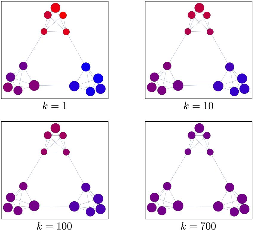
The opinion trajectories for this example are shown in Fig. 2.
In the case of increasing but bounded peer pressure, we have:
Further, this limit always exists by monotone convergence. Intuitively, this means the influence of others is limited, and that personal preferences will always slightly skew the opinions of others. Again, this is consistent with social influence theories on bounded peer pressure and trade-offs with comfort level van Baaren et al. 2009; Bindel et al. 2015.
Theorem 9.
Suppose is increasing and bounded and that:
then
Proof.
The above theorem tells us that if peer pressure is increasing and bounded, the agents’ opinions converge to a fixed distribution, which may not be a consensus, but is easily computable from the initial preferences. In this case, the shape of the network is important for determining the limit distribution, as the edge weights factor into the Laplacian. This result is similar to the convergence point given in Bindel et al. 2015 where stubbornness coefficients are not presented and peer pressure is constant.
IV Convergence Rate
We analyze the convergence rate of the algorithm and obtain a secondary result on efficiency. Define the utility of these convergent points to be the sum of the stress of the agents when the state is constant. Formally:
| (5) | ||||
Define the limiting utility as:
| (6) |
The following lemma is immediately clear from the construction of the functions , the fact that is a strictly convex function and is the limit of these strictly convex functions:
Lemma 10.
The global utility function is convex. Furthermore, the fact that (i) is smooth on its entire domain and (ii) converges uniformly to , implies that is both differentiable and its derivative can be computed as the limit of the derivatives of . ∎
Using the global utility function, we can analyze the convergence rate of the update rule. From Eq. (2), we can compute:
| (7) |
Let:
| (8) |
and define . Computing the gradient of yields:
| (9) |
We conclude the update rule, Eq. (2) can be written:
| (10) |
Necessarily, is always positive definite and therefore is always a descent direction for . Moreover, and consequently is a descent direction for . Thus, the update rule is a descent algorithm, which explains the initial fast convergence toward the average (see Fig. 2). When the descent direction converges to a Newton step, a descent algorithm can be shown to converge superlinearly Bertsekas 1999. However, these steps do not converge to Newton steps. As grows large, and and consequently for large :
for . Thus, the update rule approaches a simple gradient descent. We show that a consequence of this is a linear convergence rate.
Let:
and define:
From Eq. (10) we compute:
| (11) |
Assuming as , and expanding the gradient using Eq. (5) we obtain:
| (12) |
As , we see that:
where is the diagonal weighted degree matrix. Then:
Thus we have shown:
Theorem 11.
The convergence rate of the update rule given in Eq. (2) is linear. In particular:
| (13) |
We illustrate the slow convergence on a larger example with 500 vertices organized into a scale-free graph using the Barabási-Albert Barabási and Albert 1999 graph construction algorithm. The graph and snapshots of opinion evolution are shown in Fig. 3.

.
We show the opinion trajectories for the 500 vertex scale-free network in Fig. 4(a) and illustrate Eq. (13) in Fig. 4(b).

Notice the ratio approaches as expected.
V Cost of Anarchy
Bindel et al. 2015 observe that simultaneous minimization of Eq. (1) is a game-theoretic problem and compare the total social utility in a centralized solution to a decentralized solution (Nash equilibrium); i.e., they compute a price of anarchy Roughgarden 2003; Bindel et al. 2015. To analyze the price of anarchy of this system, we cannot use the utility function in Eq. (5), as the when . Instead, we use a total utility function to compute the cost of anarchy:
Theorem 12.
The convergent point minimizes total utility if and only if .
Proof.
If converges to a finite number , then the total utility is
Note that this is identical to the work in Bindel et al. 2015, except with edge weights multiplied by . We note that is the Nash Equilibrium used in Bindel et al. 2015. From the work in Bindel et al. 2015 we may conclude the convergent point is not optimal for finite .
If , then if for some constant , then , so grows without bound. However, for any , we have that , so . By first order necessary conditions of optimality:
minimizes , and thus is optimal. ∎
This gives the following trivial corollary, which is consistent with the work in Bindel et al. 2015.
Corollary 13.
The cost of anarchy is if and only if . ∎
VI Empirical Analysis
The hypothesis of increasing peer pressure in social settings underlies this work. We attempt to (in)validate the hypothesis that peer-pressure does increase in real-world systems, by using data from the well-known Social Evolution Experiment Madan et al. 2012. The experiment tracked the everyday life of approximately 80 students in an undergraduate dormitory over 6 months using mobile phones and surveys, in order to mine spatio-temporal behavioral patterns and the co-evolution of individual behaviors and social network structure.
The dataset includes proximity, location, and call logs, collected through a mobile application. Also included are sociometric survey data for relationships, political opinions, recent smoking behavior, attitudes towards exercise and fitness, attitudes towards diet, attitudes towards academic performance, current confidence and anxiety level, and musical tastes.
The derived social network graph (shown Fig. 5) represents each student as a node; an edge is present between two nodes if either student noted any level of interaction during the surveys. Edge weights were derived based on the level of interaction recorded between the students in the surveys, as well as the number of surveys in which the interaction appeared.

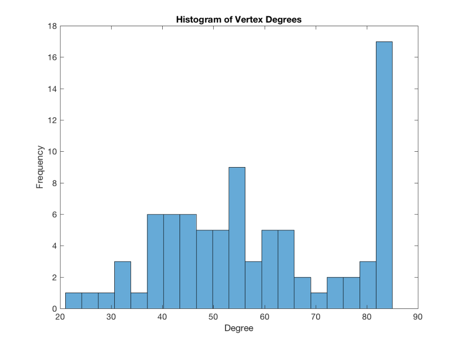
We note that this graph is not scale-free, as is typical of social networks. This may be a result of the size of the network, collection bias or simply representative of this social network. As a consequence, it is dense.
Political opinion was modeled on a scale, with lower numbers representing Republican preferences and higher numbers representing Democratic preferences. Individual scores were assigned based on reported political party, preferred candidate and likelihood of voting (prior to the election), as well as who they voted for and their approval rating of Barack Obama (after the election). Appendix A contains the code used to set these preferences. Each month’s survey was examined individually to put together a monthly time line of each person’s political views. The results of the first survey were used as proxy for their inherent personal preference, prior to peer influence.
Finally, individual stubbornness/lack of susceptibility to peer pressure was approximated using reported interest in politics on the first survey administered, as well as stated likelihood of voting. These survey questions were independent of those used in determining political preferences. Appendix B contains the code used to set stubbornness.
Given a list of , students’ preferences were simulated by aligning each iteration of play to one day in the survey period. The simulated preferences were compared to the surveyed preferences at each month, and the distances between the vectors were summed to get a single score for each list of .
This function of was minimized with fminsearch in Matlab and the best-fit peer pressure values were found to be increasing, with a best fit line and (see Fig. 6).
The inferred increasing in peer pressure is consistent with the underlying hypothesis of the paper, under the assumption that the process of repeated opinion averaging with stubbornness is a valid model of human behavior. We discuss this further in Section VII.
VII Conclusion
In this paper we study an opinion formation model under the presence of increasing peer pressure. As in earlier work, we consider agents whose opinion is affected by unchanging innate beliefs. In this paper, the relative strength of these innate beliefs may vary from agent to agent. We show that in the case of unbounded peer-pressure, opinion consensus to a weighted average of innate beliefs is ensured. We also consider the case when peer-pressure is increasing, but bounded. Simulation suggests a numerically slow convergence, which is explained by showing the system dynamics converge to gradient descent applied to a certain convex function. Using this observation we show that that convergence is linear. We evaluate our hypothesis that peer-pressure increases in real world closed systems by fitting our model to a live data set.
We note that that the assumption of a non-constant (and increasing) peer-pressure coefficient can help mitigate the fast initial convergence of this class of models. It is rare in the real-world to see dramatic opinion shifts over extremely short time scales. Such dramatic shifts are consistent with a gradient descent. However, by varying peer-pressure, the gradient descent can be controlled, leading to more consistency with real-world phenomena as illustrated.
In future work, the limitation that the network is undirected and symmetric should be removed to account for asymmetric social influence. In addition, the network is assumed to remain static during the convergence process, with connections independent of the agents’ opinions. Sufficiently different opinions could cause enough stress between agents so as to cause them to reduce influence or even sever the tie between them. A dynamic network model as in Griffin et al. 2016 could accommodate this kind of network update. Finally, it would be interesting to study corresponding control problems, in which we are given a , the desired convergence point and we can control a subset of agents reporting values (), stubbornness () or initial value () to determine conditions under which opinion steering is possible. This problem becomes more interesting if the other agents attempt to determine whether certain agents are intentionally attempting to manipulate the opinion value . Of equal interest is the transient control problem in which is steered through a set under the assumption that external factors will prevent convergence in the long-run.
Acknowledgement
All authors were supported in part by the Army Research Office, under Grant W911NF-13-1-0271. A portion of CG’s work was supported by the National Science Foundation under grant number CMMI-1463482. A portion of AS’s work was supported by the National Science foundation under grant number 1453080.
Appendix A Initial Condition Code
The Matlab code below sets the initial preferences () in this experiment.
Appendix B Stubbornness Setting Code
The Matlab code below set the stubbornness coefficients () in this experiment.
References
- DeGroot (1974) M. H. DeGroot, J. American Stat. Association 69, 118 (1974).
- Friedkin and Johnsen (1990) N. E. Friedkin and E. C. Johnsen, The Journal of Mathematical Sociology 15, 193 (1990), http://dx.doi.org/10.1080/0022250X.1990.9990069 .
- Krause (2000) U. Krause, in In Communications in Difference Equations, edited by Gordon and Breach (2000) pp. 227– 236.
- Hegselmann and Krause (2002) R. Hegselmann and U. Krause, J. Artificial Soc. Social Simul. 5 (2002).
- Slanina and Lavicka (2003) F. Slanina and H. Lavicka, The European Physical Journal B - Condensed Matter and Complex Systems 35, 279 (2003).
- Ben-Naim (2005) E. Ben-Naim, Europhys. Lett. 69, 671 (2005).
- Weisbuch et al. (2005) G. Weisbuch, G. Deffuant, and F. Amblard, Physica A 353 (2005).
- Toscani (2006) G. Toscani, Commun. Math. Sci. 4, 481 (2006).
- Weisbuch (2006) G. Weisbuch, in Econophysics and Sociophysics: Trends and Perspectives, edited by B. K. Chakrabarti, A. Chakrabarti, and A. Chatterjee (Wiley, 2006) pp. 67–94.
- Lorenz (2007) J. Lorenz, Internat. J. Modern Phys. C 18, 1819 (2007).
- Blondel et al. (2009) V. D. Blondel, J. M. Hendrickx, and J. N. Tsitsiklis, IEEE Transactions on Automatic Control 54, 2586 (2009).
- Castellano et al. (2009) C. Castellano, S. Fortunato, and V. Loreto, Rev. Modern Phys. 81, 591 (2009).
- Kurz and Rambau (2011) S. Kurz and J. Rambau, J. Difference Equ. Appl. 17, 859 (2011).
- Duering et al. (2012) B. Duering, P. Markowich, J. F. Pietschmann, and M. T. Wolfram, Proc. R. Soc. Lond. Ser. A 465 (2012).
- Canuto et al. (2012) C. Canuto, F. Fagnani, and P. Tilli, SIAM J. Contr. and Opt. , 243 (2012).
- Jabin and Motsch (2014) P.-E. Jabin and S. Motsch, Journal of Differential Equations 257, 4165 (2014).
- Dandekar et al. (2013) P. Dandekar, A. Goel, and D. T. Lee, Proceedings of the National Academy of Sciences 110, 5791 (2013), http://www.pnas.org/content/110/15/5791.full.pdf .
- Bindel et al. (2015) D. Bindel, J. Kleinberg, and S. Oren, Games and Economic Behavior 92, 248 (2015).
- Bhawalkar et al. (2013) K. Bhawalkar, S. Gollapudi, and K. Munagala, in Proceedings of the Forty-fifth Annual ACM Symposium on Theory of Computing, STOC ’13 (ACM, New York, NY, USA, 2013) pp. 41–50.
- Toner and Tu (1998) J. Toner and Y. Tu, Physical Review E 58, 4828 (1998).
- Cucker and Smale (2007) F. Cucker and S. Smale, IEEE Transactions on Automatic Control 52, 852 (2007).
- Motsch and Tadmor (2014) S. Motsch and E. Tadmor, SIAM Review 56, 577 (2014).
- Chae et al. (2015) D. H. Chae, S. Clouston, M. L. Hatzenbuehler, M. R. Kramer, H. L. F. Cooper, S. M. Wilson, S. I. Stephens-Davidowitz, R. S. Gold, and B. G. Link, PLOS ONE 10, 1 (2015).
- Stephens-Davidowitz (2017) S. Stephens-Davidowitz, Everybody Lies: Big Data, New Data, and What the Internet Can Tell Us About Who We Really Are (Dey Street Books, 2017).
- Stephens-Davidowitz (2014) S. Stephens-Davidowitz, Journal of Public Economics 118, 26 (2014).
- Niu (2013) H.-J. Niu, Journal of Applied Social Psychology 43, 1228 (2013).
- Catalini and Tucker (2016) C. Catalini and C. Tucker, Seeding the S-Curve? The Role of Early Adopters in Diffusion, Working Paper 22596 (National Bureau of Economic Research, 2016).
- Bapna and Umyarov (2015) R. Bapna and A. Umyarov, Management Science 61, 1902 (2015), http://dx.doi.org/10.1287/mnsc.2014.2081 .
- Chen (2012) X. Chen, Child Development Perspectives 6, 27 (2012).
- Rajtmajer et al. (2016) S. Rajtmajer, A. Squicciarini, C. Griffin, S. Karumanchi, and A. Tyagi, in Proceedings of the 2016 International Conference on Autonomous Agents & Multiagent Systems (2016) pp. 680–688.
- Hong and Espelage (2012) J. S. Hong and D. L. Espelage, Aggression and Violent Behavior 17, 311 (2012).
- Christakis and Fowler (2007) N. A. Christakis and J. H. Fowler, New England Journal of Medicine 357, 370 (2007), pMID: 17652652, http://dx.doi.org/10.1056/NEJMsa066082 .
- Renna et al. (2008) F. Renna, I. B. Grafova, and N. Thakur, Economics & Human Biology 6, 377 (2008), symposium on the Economics of Obesity.
- Mednick et al. (2010) S. C. Mednick, N. A. Christakis, and H. J. Fowler, PLoS ONE 5 (2010).
- Harakeh and Vollebergh (2012) Z. Harakeh and W. A. Vollebergh, Drug and Alcohol Dependence 121, 220 (2012).
- Friedkin (2006) N. E. Friedkin, A structural theory of social influence, Vol. 13 (Cambridge University Press, 2006).
- Brewer (1991) M. B. Brewer, Personality and Social Psychology Bulletin 17, 475 (1991).
- van Baaren et al. (2009) R. van Baaren, L. Janssen, T. L. Chartrand, and A. Dijksterhuis, Philosophical Trans. of the Royal Society B 364, 2381 (2009).
- Gill (1991) J. Gill, Applied Numerical Mathematics 8, 469 (1991).
- Godsil and Royle (2001) C. Godsil and G. Royle, Algebraic Graph Theory (Springer, 2001).
- Royden and Fitzpatrick (2009) H. L. Royden and P. M. Fitzpatrick, Real Analysis, 4th ed. (Pearson, 2009).
- Lorentzen (1990) L. Lorentzen, J. Computational and Applied Mathematics 32, 169 (1990).
- Bertsekas (1999) D. P. Bertsekas, Nonlinear Programming, 2nd ed. (Athena Scientific, 1999).
- Barabási and Albert (1999) A. Barabási and R. Albert, Science 286, 509 (1999).
- Roughgarden (2003) T. Roughgarden, J. Computer and System Sciences 67, 341 (2003).
- Madan et al. (2012) A. Madan, M. Cebrian, S. Moturu, K. Farrahi, and A. Pentland, IEEE Pervasive Computing 11, 36 (2012).
- Griffin et al. (2016) C. Griffin, S. Rajtamajer, A. Squicciarini, and A. Belmonte, Submitted to SIAM J. Applied Dynamical Systems (2016).