A Unified Approach for Drawdown (Drawup) of Time-Homogeneous Markov Processes

David Landriault ^†^†thanks: Department of Statistics and Actuarial Science, University of Waterloo, Waterloo, ON, N2L 3G1, Canada (dlandria@uwaterloo.ca) Bin Li ^†^†thanks: Corresponding Author: Department of Statistics and Actuarial Science, University of Waterloo, Waterloo, ON, N2L 3G1, Canada (bin.li@uwaterloo.ca) Hongzhong Zhang ^†^†thanks: Department of IEOR, Columbia University, New York, NY, 10027, USA (hz2244@columbia.edu)

August 24, 2026

Abstract

Drawdown (resp. drawup) of a stochastic process, also referred as the reflected process at its supremum (resp. infimum), has wide applications in many areas including financial risk management, actuarial mathematics and statistics. In this paper, for general time-homogeneous Markov processes, we study the joint law of the first passage time of the drawdown (resp. drawup) process, its overshoot, and the maximum of the underlying process at this first passage time. By using short-time pathwise analysis, under some mild regularity conditions, the joint law of the three drawdown quantities is shown to be the unique solution to an integral equation which is expressed in terms of fundamental two-sided exit quantities of the underlying process. Explicit forms for this joint law are found when the Markov process has only one-sided jumps or is a Lévy process (possibly with two-sided jumps). The proposed methodology provides a unified approach to study various drawdown quantities for the general class of time-homogeneous Markov processes.

Keywords: Drawdown; Integral equation; Reflected process; Time-homogeneous Markov process

MSC(2000): Primary 60G07; Secondary 60G40

1 Introduction

We consider a time-homogeneous, real-valued, non-explosive, càdlàg Markov process $X=(X_{t})_{t\geq 0}$ with state space $\mathbb{R}$ ¹¹ 1 The state space can sometimes be relaxed to an open interval of $\mathbb{R}$ (e.g., (0,+ $\infty$ ) for geometric Brownian motions). It is also possible to treat some general state space with complex boundary behaviors. However, for simplicity, we choose $\mathbb{R}$ as the state space of $X$ in this paper. defined on a filtered probability space $(\Omega,\mathcal{F},\boldsymbol{F}=(\mathcal{F}_{t})_{t\geq 0},\mathbb{P})$ with a complete and right-continuous filtration. Throughout, we silently assume that $X$ satisfies the strong Markov property (see Section III.8,9 of Rogers and Williams [33]), and exclude Markov processes with monotone paths. The first passage time of $X$ above (below) a level $x\in\mathbb{R}$ is denoted by

{\color[rgb]{0,0,0}T_{x}^{+(-)}=\inf\left\{t\geq 0:X_{t}>(<)x\right\},}

with the common convention that $\inf\emptyset=\infty$ .

The drawdown process of $X$ (also known as the reflected process of $X$ at its supremum) is denoted by $Y=(Y_{t})_{t\geq 0}$ with $Y_{t}=M_{t}-X_{t},$ where $M_{t}=\sup_{0\leq s\leq t}X_{t}$ . Let $\tau_{a}=\inf\{t>0:Y_{t}>a\}$ be the first time the magnitude of drawdowns exceeds a given threshold $a>0$ . Note that $\left({\color[rgb]{0,0,0}\sup_{0\leq s\leq t}}Y_{s}>a\right)=\left(\tau_{a}\leq t\right)$ $\mathbb{P}$ -a.s. Hence, the distributional study of the maximum drawdown of $X$ is equivalent to the study of the stopping time $\tau_{a}$ . Similarly, the drawup process of $X$ is defined as $\hat{Y}_{t}=X_{t}-m_{t}$ for $t\geq 0,$ where $m_{t}=\inf_{0\leq s\leq t}X_{t}$ . However, given that the drawup of $X$ can be investigated via the drawdown of $-X$ , we exclusively focus on the drawdown process $Y$ in this paper.

Applications of drawdowns can be found in many areas. For instance, drawdowns are widely used by mutual funds and commodity trading advisers to quantify downside risks. Interested readers are referred to Schuhmacher and Eling [34] for a review of drawdown-based performance measures. An extensive body of literature exists on the assessment and mitigation of drawdown risks (e.g., Grossman and Zhou [13], Carr et al. [7], Cherny and Obloj [8], and Zhang et al. [42]). Drawdowns are also closely related to many problems in mathematical finance, actuarial science and statistics such as the pricing of Russian options (e.g., Shepp and Shiryaev [35], Asmussen et al. [2] and Avram et al. [3]), De Finetti’s dividend problem (e.g., Avram et al. [4] and Loeffen [26]), loss-carry-forward taxation models (e.g., Kyprianou and Zhou [22] and Li et al. [25]), and change-point detection methods (e.g., Poor and Hadjiliadis [31]). More specifically, in De Finetti’s dividend problem under a fixed dividend barrier $a>0$ , the underlying surplus process with dividend payments is a process obtained from reflecting $X$ at a fixed barrier $a$ (the reflected process’ dynamics may be different than the drawdown process $Y$ when the underlying process $X$ is not spatial homogeneous). However, the distributional study of ruin quantities in De Finetti’s dividend problem can be transformed to the study of drawdown quantities for the underlying surplus process; see Kyprianou and Palmowski [21] for a more detailed discussion. Similarly, ruin problems in loss-carry-forward taxation models can also be transformed to a generalized drawdown problem for classical models without taxation, where the generalized drawdown process is defined in the form of $Y_{t}=\gamma(M_{t})-X_{t}$ for some measurable function $\gamma(\cdot)$ .

The distributional study of drawdown quantities is not only of theoretical interest, but also plays a fundamental role in the aforementioned applications. Early distributional studies on drawdowns date back to Taylor [36] on the joint Laplace transform of $\tau_{a}$ and $M_{\tau_{a}}$ for Brownian motions. This result was later generalized by Lehoczky [24] to time-homogeneous diffusion processes. Douady et al. [9] and Magdon et al. [27] derived infinite series expansions for the distribution of $\tau_{a}$ for a standard Brownian motion and a drifted Brownian motion, respectively. For spectrally negative Lévy processes, Mijatovic and Pistorius [28] obtained a sextuple formula for the joint Laplace transform of $\tau_{a}$ and the last reset time of the maximum prior to $\tau_{a}$ , together with the joint distribution of the running maximum, the running minimum, and the overshoot of $Y$ at $\tau_{a}$ . For some studies on the joint law of drawdown and drawup of spectrally negative Lévy processes or diffusion processes, please refer to Pistorius [30], Pospisil et al. [32], Zhang and Hadjiliadis [41], and Zhang [40].

As mentioned above, Lévy processes²² 2 Most often, one-sided Lévy processes (an exception to this is Baurdoux [5] for general Lévy processes) and time-homogeneous diffusion processes are two main classes of Markov processes for which various drawdown problems have been extensively studied. The treatment of these two classes of Markov processes has typically been considered distinctly in the literature. For Lévy processes, Itô’s excursion theory is a powerful approach to handle drawdown problems (e.g., Avram et al. [3], Pistorius [30], and Mijatovic and Pistorius [28]). However, the excursion-theoretic approach is somewhat specific to the underlying model, and additional care is required when a more general class of Markov processes is considered. On the other hand, for time-homogeneous diffusion processes, Lehoczky [24] introduced an ingenious approach which has recently been generalized by many researchers (e.g., Zhou [43], Li et al. [25], and Zhang [40]). Here again, Lehoczky’s approach relies on the continuity of the sample path of the underlying model, and hence is not applicable for processes with upward jumps. Also, other general methodologies (such as the martingale approach in, e.g., Asmussen [2] and the occupation density approach in, e.g., Ivanovs and Palmowski [14]) are well documented in the literature but they strongly depend on the specific structure of the underlying process. To the best of our knowledge, no unified treatment of drawdowns (drawups) for general Markov processes has been proposed in the literature.

In this paper, we propose a general and unified approach to study the joint law of $(\tau_{a},M_{\tau_{a}},Y_{\tau_{a}})$ for time-homogeneous Markov processes with possibly two-sided jumps. Under mild regularity conditions, the joint law is expressed as the solution to an integral equation which involves two-sided exit quantities of the underlying process $X$ . The uniqueness of the integral equation for the joint law is also investigated. In particular, the joint law possesses explicit forms when $X$ has only one-sided jumps or is a Lévy process (possibly with two-sided jumps). In general, our main result reduces the drawdown problem to fundamental two-sided exit quantities.

The main idea of our proposed approach is briefly summarized below. By analyzing the evolution of sample paths over a short time period following time $0$ and using renewal arguments, we first establish tight upper and lower bounds for the joint law of $(\tau_{a},M_{\tau_{a}},Y_{\tau_{a}})$ in terms of the two-sided exit quantities. Then, under mild regularity conditions, we use a Fatou’s lemma with varying measures to show that the upper and lower bounds converge when the length of the time interval approaches $0$ . This leads to an integro-differential equation satisfied by the desired joint law. Finally, we reduce the integro-differential equation to an integral equation. When $X$ is a spectrally negative Markov process or a general Lévy process, the integral equation can be solved and the joint law of $(\tau_{a},M_{\tau_{a}},Y_{\tau_{a}})$ is hence explicitly expressed in terms of two-sided exit quantities.

The rest of the paper is organized as follows. In Section 2, we introduce some fundamental two-sided exit quantities and present several preliminary results. In Section 3, we derive the joint law of $(\tau_{a},Y_{\tau_{a}},M_{\tau_{a}})$ for general time-homogeneous Markov processes. Several Markov processes for which the proposed regularity conditions are met are further discussed. Some numerical examples are investigated in more detail in Section 4. Some technical proofs are postponed to Appendix.

2 Preliminary

For ease of notation, we adopt the following conventions throughout the paper. We denote by $\mathbb{P}_{x}$ the law of $X$ given $X_{0}=x\in\mathbb{R}$ and write $\mathbb{P}\equiv\mathbb{P}_{0}$ for brevity. We write $u\wedge v=\min\{u,v\}$ , $\mathbb{R}_{+}=[0,\infty)$ , and $\int_{x}^{y}\cdot\mathrm{d}z$ for an integral on the open interval $z\in(x,y)$ .

For $q,s\geq 0$ , $u\leq x\leq v$ and $z>0$ , we introduce the following two-sided exit quantities of $X$ :

	$\displaystyle B_{1}^{(q)}(x;u,v)$	$\displaystyle:=\mathbb{E}_{x}\left[e^{-qT_{v}^{+}}1_{\left\{T_{v}^{+}<\infty,T_{v}^{+}<T_{u}^{-},X_{T_{v}^{+}}=v\right\}}\right],$
	$\displaystyle B_{2}^{(q)}(x,\mathrm{d}z;u,v)$	$\displaystyle:=\mathbb{E}_{x}\left[e^{-qT_{v}^{+}}1_{\left\{T_{v}^{+}<\infty,T_{v}^{+}<T_{u}^{-},X_{T_{v}^{+}}-v\in\mathrm{d}z\right\}}\right],$
	$\displaystyle C^{(q,s)}(x;u,v)$	$\displaystyle:=\mathbb{E}_{x}\left[e^{-qT_{u}^{-}-s(u-X_{T_{u}^{-}})}1_{\left\{T_{u}^{-}<\infty,T_{u}^{-}<T_{v}^{+}\right\}}\right].$

We also define the joint Laplace transform

B^{(q,s)}(x;u,v):=\mathbb{E}_{x}\left[e^{-qT_{v}^{+}-s(X_{T_{v}^{+}}-v)}1_{\left\{T_{v}^{+}<\infty,T_{v}^{+}<T_{u}^{-}\right\}}\right]=B_{1}^{(q)}(x;u,v)+B_{2}^{(q,s)}(x;u,v),

(2.1)

where $B_{2}^{(q,s)}(x;u,v):=\int_{0}^{\infty}e^{-sz}B_{2}^{(q)}(x,\mathrm{d}z;u,v)$ .

The following pathwise inequalities are central to the construction of tight bounds for the joint law of the triplet $(\tau_{a},M_{\tau_{a}},Y_{\tau_{a}})$ .

Proposition 2.1

For $q,s\geq 0$ , $x\in\mathbb{R}$ and $\varepsilon\in(0,a)$ , we have $\mathbb{P}_{x}$ -a.s.

1_{\{T_{x+\varepsilon}^{+}<\infty,T_{x+\varepsilon}^{+}<T_{x+\varepsilon-a}^{-}\}}\leq 1_{\{T_{x+\varepsilon}^{+}<\infty,T_{x+\varepsilon}^{+}<\tau_{a}\}}\leq 1_{\{T_{x+\varepsilon}^{+}<\infty,T_{x+\varepsilon}^{+}<T_{x-a}^{-}\}},

(2.2)

and

	$\displaystyle e^{-q\tau_{a}-s(Y_{\tau_{a}}-a)}1_{\left\{\tau_{a}<\infty,\tau_{a}<T_{x+\varepsilon}^{+}\right\}}$	$\displaystyle\geq e^{-qT_{x-a}^{-}-s(x-a-X_{T_{x-a}^{-}})-s\varepsilon}1_{\{T_{x-a}^{-}<\infty,T_{x-a}^{-}<T_{x+\varepsilon}^{+}\}},$		(2.3)
	$\displaystyle e^{-q\tau_{a}-s(Y_{\tau_{a}}-a)}1_{\left\{\tau_{a}<\infty,\tau_{a}<T_{x+\varepsilon}^{+}\right\}}$	$\displaystyle\leq e^{-qT_{x+\varepsilon-a}^{-}-s(x-a-X_{T_{x+\varepsilon-a}^{-}})}1_{\{T_{x+\varepsilon-a}^{-}<\infty,T_{x+\varepsilon-a}^{-}<T_{x+\varepsilon}^{+}\}}.$		(2.4)

Proof. By analyzing the sample paths of $X$ , it is easy to see that, for any path $\omega\in(T_{x+\varepsilon}^{+}<\infty)$ , we have $\mathbb{P}_{x}\{\tau_{a}\leq T_{x-a}^{-}\}=1$ , so

(T_{x+\varepsilon}^{+}<\infty,T_{x+\varepsilon}^{+}<\tau_{a})=(T_{x+\varepsilon}^{+}<\infty,T_{x+\varepsilon}^{+}<\tau_{a}\leq T_{x-a}^{-})\subset(T_{x+\varepsilon}^{+}<\infty,T_{x+\varepsilon}^{+}<T_{x-a}^{-})\quad\mathbb{P}_{x}\text{-a.s.}

and similarly, $\mathbb{P}_{x}$ -a.s.

(T_{x+\varepsilon}^{+}<\infty,T_{x+\varepsilon}^{+}<T_{x+\varepsilon-a}^{-})=(T_{x+\varepsilon}^{+}<\infty,T_{x+\varepsilon}^{+}<T_{x+\varepsilon-a}^{-},T_{x+\varepsilon}^{+}<\tau_{a})\subset(T_{x+\varepsilon}^{+}<\infty,T_{x+\varepsilon}^{+}<\tau_{a}),

which immediately implies (2.2). On the other hand, by using the same argument, we have

(T_{x-a}^{-}<\infty,T_{x-a}^{-}<T_{x+\varepsilon}^{+})=(T_{x-a}^{-}<\infty,\tau_{a}\leq T_{x-a}^{-}<T_{x+\varepsilon}^{+})\subset(\tau_{a}<\infty,\tau_{a}<T_{x+\varepsilon}^{+})\quad\mathbb{P}_{x}\text{-a.s.}

(2.5)

and

(\tau_{a}<\infty,\tau_{a}<T_{x+\varepsilon}^{+})=(\tau_{a}<\infty,T_{x+\varepsilon-a}^{-}\leq\tau_{a}<T_{x+\varepsilon}^{+})\subset(T_{x+\varepsilon-a}^{-}<\infty,T_{x+\varepsilon-a}^{-}<T_{x+\varepsilon}^{+})\quad\mathbb{P}_{x}\text{-a.s.}

(2.6)

For any path $\omega\in(T_{x-a}^{-}<\infty,T_{x-a}^{-}<T_{x+\varepsilon}^{+})$ , we know from (2.5) that $\omega\in(T_{x-a}^{-}<\infty,\tau_{a}\leq T_{x-a}^{-}<T_{x+\varepsilon}^{+})$ . This implies $M_{\tau_{a}}(\omega)\leq x+\varepsilon$ and $X_{\tau_{a}}(\omega)\geq X_{T_{x-a}^{-}}(\omega)$ , which further entails that $Y_{\tau_{a}}(\omega)=M_{\tau_{a}}(\omega)-X_{\tau_{a}}(\omega)\leq x+\varepsilon-X_{T_{x-a}^{-}}(\omega)$ . Therefore, by the above analysis and the second inequality of (2.2),

e^{-qT_{x-a}^{-}-s(x+\varepsilon-X_{T_{x-a}^{-}})}1_{\left\{T_{x-a}^{-}<\infty,T_{x-a}^{-}<T_{x+\varepsilon}^{+}\right\}}\leq e^{-q\tau_{a}-sY_{\tau_{a}}}1_{\left\{\tau_{a}<\infty,\tau_{a}<T_{x+\varepsilon}^{+}\right\}}\quad\mathbb{P}_{x}\text{-a.s.}

which naturally leads to (2.3).

Similarly, for any sample path $\omega\in(\tau_{a}<\infty,\tau_{a}<T_{x+\varepsilon}^{+})$ , we know from (2.6) that $\omega\in(\tau_{a}<\infty,T_{x+\varepsilon-a}^{-}\leq\tau_{a}<T_{x+\varepsilon}^{+})$ , which implies that $x-X_{T_{x+\varepsilon-a}^{-}}(\omega)\leq Y_{T_{x+\varepsilon-a}^{-}}(\omega)\leq Y_{\tau_{a}}(\omega).$ Therefore, by the first inequality of (2.2), we obtain

e^{-q\tau_{a}-sY_{\tau_{a}}}1_{\left\{\tau_{a}<\infty,\tau_{a}<T_{x+\varepsilon}^{+}\right\}}\leq e^{-qT_{x+\varepsilon-a}^{-}-s(x-X_{T_{x+\varepsilon-a}^{-}})}1_{\{T_{x+\varepsilon-a}^{-}<\infty,T_{x+\varepsilon-a}^{-}<T_{x+\varepsilon}^{+}\}}\quad\mathbb{P}_{x}\text{-a.s.}

This implies the second inequality of (2.4).

By Proposition 2.1, we easily obtain the following useful estimates.

Corollary 2.1

For $q,s\geq 0$ , $x\in\mathbb{R},z>0$ and $\varepsilon\in(0,a)$ ,

	$\displaystyle B_{1}^{(q)}(x;x+\varepsilon-a,x+\varepsilon)$	$\displaystyle\leq\mathbb{E}_{x}\left[e^{-qT_{x+\varepsilon}^{+}}1_{\{T_{x+\varepsilon}^{+}<\infty,T_{x+\varepsilon}^{+}<\tau_{a},X_{T_{x+\varepsilon}^{+}}=x+\varepsilon\}}\right]\leq B_{1}^{(q)}(x;x-a,x+\varepsilon),$
	$\displaystyle B_{2}^{(q)}(x,\mathrm{d}z;x+\varepsilon-a,x+\varepsilon)$	$\displaystyle\leq\mathbb{E}_{x}\left[e^{-qT_{x+\varepsilon}^{+}}1_{\{T_{x+\varepsilon}^{+}<\infty,T_{x+\varepsilon}^{+}<\tau_{a},X_{T_{x+\varepsilon}^{+}}-x-\varepsilon\in\mathrm{d}z\}}\right]\leq B_{2}^{(q)}(x,\mathrm{d}z;x-a,x+\varepsilon),$

and

e^{-s\varepsilon}C^{(q,s)}(x;x-a,x+\varepsilon)\leq\mathbb{E}_{x}\left[e^{-q\tau_{a}-s(Y_{\tau_{a}}-a)}1_{\left\{\tau_{a}<\infty,\tau_{a}<T_{x+\varepsilon}^{+}\right\}}\right]\leq e^{s\varepsilon}C^{(q,s)}(x;x+\varepsilon-a,x+\varepsilon).

Remark 2.1

It is not difficult to check that the results of Proposition 2.1 and Corollary 2.1 still hold if the first passage times and the drawdown times are only observed discretely or randomly (such as the Poisson observation framework in Albrecher et al. [1] for the latter). Further, explicit relationship between Poisson observed first passage times and Poisson observed drawdown times (similar as for Theorem 3.1 below) can be found by exploiting the same approach as laid out in this paper.

The later analysis involves the weak convergence of measures which is recalled here. Consider a metric space $S$ with the Borel $\sigma$ -algebra on it. We say a sequence of finite measures $\{\mu_{n}\}_{n\in\mathbb{N}}$ is weakly convergent to a finite measure $\mu$ as $n\rightarrow\infty$ if

\lim_{n\rightarrow\infty}\int_{S}\phi(z)\mathrm{d}\mu_{n}(z)=\int_{S}\phi(z)\mathrm{d}\mu(z),

for any bounded and continuous function $\phi(\cdot)$ on $S$ .

In the next lemma, we show some forms of Fatou’s lemma for varying measures under weak convergence. Similar results are proved in Feinberg et al. [10] for probability measures. For completeness, a proof for general finite measures is provided in Appendix.

Lemma 2.1

Suppose that $\{\mu_{n}\}_{n\in\mathbb{N}}$ is a sequence of finite measures on $S$ which is weakly convergent to a finite measure $\mu$ , and $\{\phi_{n}\}_{n\in\mathbb{N}}$ is a sequence of uniformly bounded and nonnegative functions on $S$ . Then,

\int_{S}\liminf_{n\rightarrow\infty,w\rightarrow z}\phi_{n}(w)\mathrm{d}\mu(z)\leq\liminf_{n\rightarrow\infty}\int_{S}\phi_{n}(z)\mathrm{d}\mu_{n}(z)\text{,}

(2.7)

and

\int_{S}\limsup_{n\rightarrow\infty,w\rightarrow z}\phi_{n}(w)\mathrm{d}\mu(z)\geq\limsup_{n\rightarrow\infty}\int_{S}\phi_{n}(z)\mathrm{d}\mu_{n}(z).

(2.8)

3 Main results

In this section, we study the joint law of $(\tau_{a},M_{\tau_{a}},Y_{\tau_{a}})$ for a general Markov process with possibly two-sided jumps. The following assumptions on the two-sided exit quantities of $X$ are assumed to hold, which are sufficient (but not necessary) conditions for the applicability of our proposed methodology. Weaker assumptions might be assumed for special Markov processes; see, for instance, Remark 3.3 and Corollary 3.1 below.

Assumption 3.1

For all $q,s\geq 0$ , $z>0$ and $x>X_{0}$ , we assume the following limits exist and identities hold:

	$\displaystyle\text{{(A1)} }b_{a,1}^{(q)}(x)$	$\displaystyle:=\lim_{\varepsilon\downarrow 0}\frac{1-B_{1}^{(q)}(x;x-a,x+\varepsilon)}{\varepsilon}=\lim_{\varepsilon\downarrow 0}\frac{1-B_{1}^{(q)}(x;x+\varepsilon-a,x+\varepsilon)}{\varepsilon}$
		$\displaystyle=\lim_{\varepsilon\downarrow 0}\frac{1-B_{1}^{(q)}(x-\varepsilon;x-a,x)}{\varepsilon}=\lim_{\varepsilon\downarrow 0}\frac{1-B_{1}^{(q)}(x-\varepsilon;x-\varepsilon-a,x)}{\varepsilon},$

and $\int_{x}^{y}b_{a,1}^{(q)}(w)\mathrm{d}w<\infty$ for any $x,y\in\mathbb{R}$ ;

	$\displaystyle\text{{(A2)} }b_{a,2}^{(q,s)}(x)$	$\displaystyle:=\lim_{\varepsilon\downarrow 0}\frac{1}{\varepsilon}B_{2}^{(q,s)}(x;x-a,x+\varepsilon)=\lim_{\varepsilon\downarrow 0}\frac{1}{\varepsilon}B_{2}^{(q,s)}(x;x+\varepsilon-a,x+\varepsilon)$
		$\displaystyle=\lim_{\varepsilon\downarrow 0}\frac{1}{\varepsilon}B_{2}^{(q,s)}(x-\varepsilon;x-a,x)=\lim_{\varepsilon\downarrow 0}\frac{1}{\varepsilon}B_{2}^{(q,s)}(x-\varepsilon;x-\varepsilon-a,x),$

and $s\longmapsto b_{a,2}^{(q,s)}(x)$ is right continuous at $s=0$ ;

	$\displaystyle\text{{(A3)} }c_{a}^{(q,s)}(x)$	$\displaystyle:=\lim_{\varepsilon\downarrow 0}\frac{C^{(q,s)}(x;x-a,x+\varepsilon)}{\varepsilon}=\lim_{\varepsilon\downarrow 0}\frac{C^{(q,s)}(x;x+\varepsilon-a,x+\varepsilon)}{\varepsilon}$
		$\displaystyle=\lim_{\varepsilon\downarrow 0}\frac{C^{(q,s)}(x-\varepsilon;x-a,x)}{\varepsilon}=\lim_{\varepsilon\downarrow 0}\frac{C^{(q,s)}(x-\varepsilon;x-\varepsilon-a,x)}{\varepsilon}.$

Under Assumptions (A1) and (A2), it follows from (2.1) that

b_{a}^{(q,s)}(x):=\lim_{\varepsilon\downarrow 0}\frac{1-B^{(q,s)}(x;x-a,x+\varepsilon)}{\varepsilon}=b_{a,1}^{(q)}(x)-b_{a,2}^{(q,s)}(x).

(3.1)

Remark 3.1

Due to the general structure of $X$ , it is difficult to refine Assumptions (A1)-(A3) unless a specific structure for $X$ is given. A necessary condition for Assumptions (A1)-(A3) to hold is that,

T_{x}^{+}=0\text{ and }X_{T_{x}^{+}}=x,\text{ }\mathbb{P}_{x}\text{-a.s. for all }x\in\mathbb{R}\text{.}

In other words, $X$ must be upward regular and creeping upward at every $x$ .³³ 3 See page 142 and page 197 of [19] for definitions of regularity and creeping for Lévy processes. In the later part of this section, we provide some examples of Markov processes which satisfy Assumptions (A1)-(A3), including spectrally negative Lévy processes, linear diffusions, piecewise exponential Markov processes, and jump diffusions.

Remark 3.2

By Theorem 5.22 of Kallenberg [16] or Proposition 7.1 of Landriault et al. [23], we know that Assumption (A2) implies that the measures $\frac{1}{\varepsilon}B_{2}^{(q)}(x,\mathrm{d}z;x-a,x+\varepsilon)$ , $\frac{1}{\varepsilon}B_{2}^{(q)}(x,\mathrm{d}z;x+\varepsilon-a,x+\varepsilon)$ , $\frac{1}{\varepsilon}B_{2}^{(q)}(x-\varepsilon,\mathrm{d}z;x-a,x)$ and $\frac{1}{\varepsilon}B_{2}^{(q)}(x-\varepsilon,\mathrm{d}z;x-\varepsilon-a,x)$ weakly converge to the same measure on $\mathbb{R}_{+}$ , denoted as $b_{a,2}^{(q)}(x,\mathrm{d}z)$ , such that $\int_{\mathbb{R}_{+}}e^{-sz}b_{a,2}^{(q)}(x,\mathrm{d}z)=b_{a,2}^{(q,s)}(x)$ . We point out that it is possible that $b_{a,2}^{(q)}(x,\{0\})>0$ , though the measure $B_{2}^{(q)}(x,\mathrm{d}z;u,v)$ is only defined on $z\in(0,\infty)$ .

We are now ready to present the main result of this paper related to the joint law of $(\tau_{a},Y_{\tau_{a}},M_{\tau_{a}})$ .

Theorem 3.1

Consider a general time-homogeneous Markov process $X$ satisfying Assumptions (A1)-(A3). For $q,s\geq 0$ and $K\in\mathbb{R}$ , let

h(x)=\mathbb{E}_{x}\left[e^{-q\tau_{a}-s(Y_{\tau_{a}}-a)}1_{\{\tau_{a}<\infty,M_{\tau_{a}}\leq K\}}\right],\quad x\leq K.

Then $h(\cdot)$ is differentiable in $x<K$ and solves the following integral equation

h(x)=\int_{x}^{K}e^{-\int_{x}^{y}b_{a,1}^{(q)}(w)\mathrm{d}w}\left(c_{a}^{(q,s)}(y)+\int_{[0,K-y)}h(y+z)b_{a,2}^{(q)}(y,\mathrm{d}z)\right)\mathrm{d}y\text{,}\quad x\leq K.

(3.2)

Proof. By the strong Markov property of $X$ , for any $X_{0}=x\leq y<K$ and $0<\varepsilon<(K-y)\wedge a$ , we have

	$\displaystyle h(y)$	$\displaystyle=\mathbb{E}_{y}\left[e^{-q\tau_{a}-s(Y_{\tau_{a}}-a)}1_{\left\{\tau_{a}<\infty,\tau_{a}<T_{y+\varepsilon}^{+}\right\}}\right]+\mathbb{E}_{y}\left[e^{-qT_{y+\varepsilon}^{+}}1_{\{T_{y+\varepsilon}^{+}<\infty,T_{y+\varepsilon}^{+}<\tau_{a},X_{T_{y+\varepsilon}^{+}}=y+\varepsilon\}}\right]h(y+\varepsilon)$
		$\displaystyle+\int_{0}^{K-y-\varepsilon}\mathbb{E}_{y}\left[e^{-qT_{y+\varepsilon}^{+}}1_{\{T_{y+\varepsilon}^{+}<\infty,T_{y+\varepsilon}^{+}<\tau_{a},X_{T_{y+\varepsilon}^{+}}-y-\varepsilon\in\mathrm{d}z\}}\right]h(y+\varepsilon+z).$

By Corollary 2.1, it follows that

	$\displaystyle h(y+\varepsilon)-h(y)$	$\displaystyle\geq-e^{s\varepsilon}C^{(q,s)}(y;y+\varepsilon-a,y+\varepsilon)+\left(1-B_{1}^{(q)}(y;y-a,y+\varepsilon)\right)h(y+\varepsilon)$
		$\displaystyle-\int_{0}^{K-y-\varepsilon}h(y+\varepsilon+z)B_{2}^{(q)}(y,\mathrm{d}z;y-a,y+\varepsilon),$		(3.3)

and

	$\displaystyle h(y+\varepsilon)-h(y)$	$\displaystyle\leq-e^{-s\varepsilon}C^{(q,s)}(y;y-a,y+\varepsilon)+\left(1-B_{1}^{(q)}(y;y+\varepsilon-a,y+\varepsilon)\right)h(y+\varepsilon)$
		$\displaystyle-\int_{0}^{K-y-\varepsilon}h(y+\varepsilon+z)B_{2}^{(q)}(y,\mathrm{d}z;y+\varepsilon-a,y+\varepsilon).$		(3.4)

By Assumptions (A1)-(A3) and $h(\cdot)\in[0,1]$ , it is clear that both the lower bound of $h(y+\varepsilon)-h(y)$ in (3.3) and the upper bound in (3.4) vanish as $\varepsilon\downarrow 0$ . Hence, $h(y)$ is right continuous for $y\in[x,K)$ . Replacing $y$ by $y-\varepsilon$ in (3.3) and (3.4), and using Assumptions (A1)-(A3) again, it follows that $h(y)$ is also left continuous for $y\in(x,K]$ with $h(K)=0$ . Therefore, $h(y)$ is continuous for $y\in[x,K]$ (left continuous at $x$ and right continuous at $K$ ).

To consecutively show the differentiability, we divide inequalities (3.3) and (3.4) by $\varepsilon$ . It follows from Assumptions (A1)-(A3), Remark 3.2, Lemma 2.1 and the continuity of $h$ that

		$\displaystyle\liminf_{\varepsilon\downarrow 0}\frac{h(y+\varepsilon)-h(y)}{\varepsilon}$
		$\displaystyle\geq-c_{a}^{(q,s)}(y)+b_{a,1}^{(q)}(y)h(y)-\limsup_{\varepsilon\downarrow 0}\int_{0}^{K-y-\varepsilon}h(y+\varepsilon+z)\frac{B_{2}^{(q)}(y,\mathrm{d}z;y-a,y+\varepsilon)}{\varepsilon}$
		$\displaystyle\geq-c_{a}^{(q,s)}(y)+b_{a,1}^{(q)}(y)h(y)-\int_{[0,K-y)}h(y+z)b_{a,2}^{(q)}(y,\mathrm{d}z)\text{,}$

and similarly,

\limsup_{\varepsilon\downarrow 0}\frac{h(y+\varepsilon)-h(y)}{\varepsilon}\leq-c_{a}^{(q,s)}(y)+b_{a,1}^{(q)}(y)h(y)-\int_{[0,K-y)}h(y+z)b_{a,2}^{(q)}(y,\mathrm{d}z).

Since the two limits coincide, one concludes that $h(y)$ is right differentiable for $y\in(x,K)$ . Moreover, by replacing $y$ by $y-\varepsilon$ in (3.3) and (3.4), and using similar arguments, we can show that $h(y)$ is also left differentiable for $y\in(x,K)$ . Since the left and right derivatives coincide, we conclude that $h(y)$ is differentiable for any $y\in(x,K)$ and solves the following ordinary integro-differential equation (OIDE),

h^{\prime}(y)-b_{a,1}^{(q)}(y)h(y)=-c_{a}^{(q,s)}(y)-\int_{[0,K-y)}h(y+z)b_{a,2}^{(q)}(y,\mathrm{d}z).

(3.5)

Multiplying both sides of (3.5) by $e^{-\int_{x}^{y}b_{a,1}^{(q)}(w)\mathrm{d}w}$ , integrating the resulting equation (with respect to $y$ ) from $x$ to $K$ , and using $h(K)=0$ , this completes the proof of Theorem 3.1.

When the Markov process $X$ is spectrally negative (i.e., with no upward jumps), the upward overshooting density $b_{a,2}^{(q)}(x,\mathrm{d}z)$ is trivially $0$ . Theorem 3.1 reduces to the following corollary.

Corollary 3.1

Consider a spectrally negative time-homogeneous Markov process $X$ satisfying Assumptions (A1) and (A3). For $q,s\geq 0$ and $K>0$ , we have

\mathbb{E}_{x}\left[e^{-q\tau_{a}-s(Y_{\tau_{a}}-a)}1_{\{\tau_{a}<\infty,M_{\tau_{a}}\leq K\}}\right]=\int_{x}^{K}e^{-\int_{x}^{y}b_{a,1}^{(q)}(w)\mathrm{d}w}c_{a}^{(q,s)}(y)\mathrm{d}y\text{,}\quad x\leq K.

When $X$ is a general Lévy process (possibly with two-sided jumps), we have the following result for the joint Laplace transform of the triplet $(\tau_{a},Y_{\tau_{a}},M_{\tau_{a}})$ . Note that Corollary 3.2 should be compared to Theorem 4.1 of Baurdoux [5], in which, under the Lévy framework, the resolvent density of $Y$ is expressed in terms of the resolvent density of $X$ using excursion theory.

Corollary 3.2

Consider a Lévy process $X$ satisfying Assumptions (A1)-(A3). For $q,s,\delta\geq 0$ , we have⁴⁴ 4 For Lévy processes $\mathbb{P}\{\tau_{a}<\infty\}=1$ as long as $X$ is not monotone.

\mathbb{E}\left[e^{-q\tau_{a}-s(Y_{\tau_{a}}-a)-\delta M_{\tau_{a}}}\right]=\frac{c_{a}^{(q,s)}(0)}{\delta+b_{a}^{(q,\delta)}(0)}.

(3.6)

Proof. By the spatial homogeneity of the Lévy process $X$ , Eq. (3.2) at $x=0$ reduces to

h(0)=\frac{c_{a}^{(q,s)}(0)}{b_{a,1}^{(q)}(0)}\left(1-e^{-b_{a,1}^{(q)}(0)K}\right)+\int_{0}^{K}e^{-b_{a,1}^{(q)}(0)y}\int_{[0,K-y)}h(y+z)b_{a,2}^{(q)}(0,\mathrm{d}z)\mathrm{d}y.

(3.7)

Let

\hat{h}(0):=\mathbb{E}\left[e^{-q\tau_{a}-s(Y_{\tau_{a}}-a)-\delta M_{\tau_{a}}}\right]=\mathbb{E}\left[e^{-q\tau_{a}-s(Y_{\tau_{a}}-a)}1_{\{M_{\tau_{a}}\leq e_{\delta}\}}\right]\text{,}

where $e_{\delta}$ is an independent exponential random variable with finite mean $1/\delta>0$ . Multiplying both sides of (3.7) by $\delta e^{-\delta K}$ , integrating the resulting equation (with respect to $K$ ) from $0$ to $\infty$ , and using integration by parts, one obtains

	$\displaystyle\hat{h}(0)$	$\displaystyle=\frac{c_{a}^{(q,s)}(0)}{\delta+b_{a,1}^{(q)}(0)}+\int_{0}^{\infty}\delta e^{-\delta K}\int_{0}^{K}e^{-b_{a,1}^{(q)}(0)y}\int_{[0,K-y)}h(y+z)b_{a,2}^{(q)}(0,\mathrm{d}z)\mathrm{d}y\mathrm{d}K$
		$\displaystyle=\frac{c_{a}^{(q,s)}(0)}{\delta+b_{a,1}^{(q)}(0)}+\int_{0}^{\infty}e^{-b_{a,1}^{(q)}(0)y}\mathrm{d}y\int_{\mathbb{R}_{+}}b_{a,2}^{(q)}(0,\mathrm{d}z)\int_{z+y}^{\infty}\delta e^{-\delta K}\mathbb{E}\left[e^{-q\tau_{a}-s(Y_{\tau_{a}}-a)}1_{\{M_{\tau_{a}}\leq K-y-z\}}\right]\mathrm{d}K$
		$\displaystyle=\frac{c_{a}^{(q,s)}(0)}{\delta+b_{a,1}^{(q)}(0)}+\hat{h}(0)\frac{\int_{\mathbb{R}_{+}}e^{-\delta z}b_{a,2}^{(q)}(0,\mathrm{d}z)}{\delta+b_{a,1}^{(q)}(0)}.$

Solving for $\hat{h}(0)$ and using (3.1), it follows that

\hat{h}(0)=\frac{c_{a}^{(q,s)}(0)}{\delta+b_{a,1}^{(q)}(0)-\int_{\mathbb{R}_{+}}e^{-\delta z}b_{a,2}^{(q)}(0,\mathrm{d}z)}=\frac{c_{a}^{(q,s)}(0)}{\delta+b_{a}^{(q,\delta)}(0)}.

It follows from the monotone convergence theorem that (3.6) also holds for $\delta=0$ .

Remark 3.3

We point out that Assumptions (A1)-(A3) are not necessary to yield (3.6) in the Lévy framework. In fact, by the spatial homogeneity of $X$ , similar to (3.3) and (3.4), we have

\frac{e^{-(s+\delta)\varepsilon}C^{(q,s)}(0;-a,\varepsilon)}{1-e^{-\delta\varepsilon}B^{(q,\delta)}(0;\varepsilon-a,\varepsilon)}\leq\mathbb{E}\left[e^{-q\tau_{a}-s(Y_{\tau_{a}}-a)-\delta M_{\tau_{a}}}\right]\leq\frac{e^{s\varepsilon}C^{(q,s)}(0;\varepsilon-a,\varepsilon)}{1-e^{-\delta\varepsilon}B^{(q,\delta)}(0;-a,\varepsilon)},

for any $\varepsilon\in(0,a)$ . Suppose that the following condition holds:

\lim_{\varepsilon\downarrow 0}\frac{C^{(q,s)}(0;-a,\varepsilon)}{1-e^{-\delta\varepsilon}B^{(q,\delta)}(0;\varepsilon-a,\varepsilon)}=\lim_{\varepsilon\downarrow 0}\frac{C^{(q,s)}(0;\varepsilon-a,\varepsilon)}{1-e^{-\delta\varepsilon}B^{(q,\delta)}(0;-a,\varepsilon)}:=D_{a}^{(q,s,\delta)}

Then,

\mathbb{E}\left[e^{-q\tau_{a}-s(Y_{\tau_{a}}-a)-\delta M_{\tau_{a}}}\right]=D_{a}^{(q,s,\delta)}.

Theorem 3.1 shows that the joint law $\mathbb{E}_{x}\left[e^{-q\tau_{a}-s(Y_{\tau_{a}}-a)}1_{\{M_{\tau_{a}}\leq K\}}\right]$ is a solution to Eq. (3.2). Furthermore, the following theorem shows that Eq. (3.2) admits a unique solution.

Theorem 3.2

Suppose that Assumptions (A1)-(A3) hold. For $q,s\geq 0$ and $K>0$ , Eq. (3.2) admits a unique solution.

Proof. From Theorem 3.1, we know that $h(x):=\mathbb{E}_{x}\left[e^{-q\tau_{a}-s(Y_{\tau_{a}}-a)}1_{\{\tau_{a}<\infty,M_{\tau_{a}}\leq K\}}\right]$ is a solution of (3.2). We also notice that any continuous solution to (3.2) must vanish when $x\uparrow$ $K$ . For any fixed $L\in(-\infty,K)$ , we define a metric space $(\mathbb{A}_{L},\boldsymbol{d}_{L})$ , where $\mathbb{A}_{L}=\left\{f\in C[L,K],f(K)=0\right\}$ and the metric $\boldsymbol{d}_{L}(f,g)=\sup_{x\in[L,K]}|f(x)-g(x)|$ for $f,g\in\mathbb{A}_{L}$ . We then define a mapping $\mathcal{L}$ on $\mathbb{A}_{L}$ by

\mathcal{L}f(x)=\int_{x}^{K}e^{-\int_{x}^{y}b_{a,1}^{(q)}(w)\mathrm{d}w}\left(c_{a}^{(q,s)}(y)+\int_{[0,K-y)}f(y+z)b_{a,2}^{(q)}(y,\mathrm{d}z)\right)\mathrm{d}y,\text{\quad}x\in[L,K],

where $f\in\mathbb{A}_{L}$ . It is clear that $\mathcal{L}(\mathbb{A}_{L})\subset\mathbb{A}_{L}$ .

Next we show that $\mathcal{L}:\mathbb{A}_{L}\rightarrow\mathbb{A}_{L}$ is a contraction mapping. By the definitions of the two-sided exit quantities, for any $y\in\mathbb{R}$ , it follows that

C^{(q,s)}(y;y-a,y+\varepsilon)+\int_{\mathbb{R}_{+}}B_{2}^{(q)}(y,\mathrm{d}z;y-a,y+\varepsilon)\leq 1-B_{1}^{(q)}(y;y-a,y+\varepsilon).

(3.8)

Dividing each term in (3.8) by $\varepsilon\in(0,a)$ and letting $\varepsilon\downarrow 0$ , it follows from Assumptions (A1)-(A3) that

0\leq c_{a}^{(q,s)}(y)+\int_{\mathbb{R}_{+}}b_{a,2}^{(q)}(y,\mathrm{d}z)\leq b_{a,1}^{(q)}(y),\quad y\in\mathbb{R}.

(3.9)

By (3.9), we have for any $f,g\in\mathbb{A}_{L}$ ,

	$\displaystyle\boldsymbol{d}_{L}\left(\mathcal{L}f,\mathcal{L}g\right)$	$\displaystyle\leq\sup_{t\in[L,K]}\left\|f(t)-g(t)\right\|\sup_{x\in[L,K]}\int_{x}^{K}e^{-\int_{x}^{y}b_{a,1}^{(q)}(w)\mathrm{d}w}\int_{\mathbb{R}_{+}}b_{a,2}^{(q)}(y,\mathrm{d}z)\mathrm{d}y$
		$\displaystyle\leq\boldsymbol{d}_{L}(f,g)\sup_{L\leq x\leq K}\int_{x}^{K}e^{-\int_{x}^{y}b_{a,1}^{(q)}(w)\mathrm{d}w}b_{a,1}^{(q)}(y)\mathrm{d}y$
		$\displaystyle\leq\boldsymbol{d}_{L}(f,g)\left(1-e^{-\int_{L}^{K}b_{a,1}^{(q)}(w)\mathrm{d}w}\right).$

Since $\int_{L}^{K}b_{a,1}^{(q)}(w)\mathrm{d}w<\infty$ by Assumption (A1), one concludes that $\mathcal{L}:\mathbb{A}_{L}\rightarrow\mathbb{A}_{L}$ is a contraction mapping. By Banach fixed point theorem, there exists a unique fixed point in $\mathbb{A}_{L}$ . By a restriction of domain, it is easy to see that $\mathbb{A}_{L_{1}}\subset\mathbb{A}_{L_{2}}$ for $-\infty<L_{1}<L_{2}<K$ . By the arbitrariness of $L$ , the uniqueness holds for the space $\cap_{L<K}\mathbb{A}_{L}$ . This completes the proof.

For the reminder of this section, we state several examples of Markov processes satisfying Assumptions (A1)-(A3). Note that the joint law of drawdown estimates for Examples 3.1 and 3.3 were solved by Mijatovic and Pistorius [28] and Lehoczky [24], respectively (using different approaches). Assumption verifications for Examples 3.4 and 3.5 are postponed to Appendix.

Example 3.1 (Spectrally negative Lévy processes)

Consider a spectrally negative Lévy process $X$ . Let $\psi(s):=\frac{1}{t}\log\mathbb{E}[e^{sX_{t}}]$ $\left(s\geq 0\right)$ be the Laplace exponent of $X$ . Further, let $W^{(q)}:\mathbb{R}\rightarrow[0,\infty)$ be the well-known $q$ -scale function of $X$ ; see, for instance Chapter 8 of Kyprianou [19]. The second scale function is defined as $Z^{(q)}(x)=1+q\int_{0}^{x}W^{(q)}(y)\mathrm{d}y$ . Under some mild conditions (e.g., Lemma 2.4 of Kuznetsov et al. [18]), the scale functions are continuously differentiable which further implies that Assumptions (A1) and (A3) hold with

b_{a,1}^{(q)}(0)=\frac{W^{(q)\prime}(a)}{W^{(q)}(a)}\text{ and }c_{a}^{(q,s)}(0)=e^{sa}\frac{Z_{s}^{(p)}(a)W_{s}^{(p)\prime}(a)-Z_{s}^{(p)\prime}(a)W_{s}^{(p)}(a)}{W_{s}^{(p)}(a)},

(3.10)

where $p=q-\psi(s)$ , and $W_{s}^{(p)}$ ( $Z_{s}^{(p)}$ ) is the (second) scale function of $X$ under a new probability measure $\mathbb{P}^{s}$ defined by the Radon-Nikodym derivative process $\left.\frac{\mathrm{d}\mathbb{P}^{s}}{\mathrm{d}\mathbb{P}}\right|_{\mathcal{F}_{t}}=e^{sX_{t}-\psi(s)t}$ for $t\geq 0$ . Therefore, by Corollary 3.2 and (3.10), we have

\mathbb{E}\left[e^{-q\tau_{a}-s(Y_{\tau_{a}}-a)-\delta M_{\tau_{a}}}\right]=\frac{e^{sa}W^{(q)}(a)}{\delta W^{(q)}(a)+W^{(q)\prime}(a)}\frac{Z_{s}^{(p)}(a)W_{s}^{(p)\prime}(a)-pW_{s}^{(p)}(a)^{2}}{W_{s}^{(p)}(a)},

which is consistent with Theorem 3.1 of Landriault et al. [23], and Theorem 1 of Mijatovic and Pistorius [28].

Example 3.2 (Refracted Lévy processes)

Consider a refracted spectrally negative Lévy process $X$ of the form

X_{t}=U_{t}-\lambda\int_{0}^{t}1_{\{X_{s}>b\}}\mathrm{d}s,

(3.11)

where $\lambda\geq 0$ , $b>0$ , and $U$ is a spectrally negative Lévy process (see Kyprianou and Loeffen [20]). Let $W^{(q)}$ ( $Z^{(q)}$ ) be the (second) $q$ -scale function of $U$ , and $\mathbb{W}^{(q)}$ be the $q$ -scale function of the process $\{U_{t}-\lambda t\}_{t\geq 0}$ . Similar to Example 3.1, all the scale functions are continuously differentiable under mild conditions.

For simplicity, we only consider the quantity $\mathbb{E}_{x}\left[e^{-q\tau_{a}}1_{\{\tau_{a}<\infty,M_{\tau_{a}}\leq K\}}\right]$ with $b>x-a$ (otherwise the problem reduces to Example 3.1 for $X_{t}=U_{t}-\lambda t$ ). By Theorem 4 of Kyprianou and Loeffen [20], one can verify that Assumptions (A1) and (A3) hold. For $b>x$ , from (3.10) with $s=0$ , we have

b_{a,1}^{(q)}(x)=\frac{W^{(q)\prime}(a)}{W^{(q)}(a)}\text{ and }c_{a}^{(q,0)}(x)=\frac{Z^{(q)}(a)W^{(q)\prime}(a)-Z^{(q)\prime}(a)W^{(q)}(a)}{W^{(q)}(a)}.

For $x>b>x-a$ ,

b_{a,1}^{(q)}(x)=\frac{\left(1+\lambda\mathbb{W}^{(q)}(0)\right)W^{(q)\prime}(a)+\lambda\int_{b-x+a}^{a}\mathbb{W}^{(q)\prime}(a-y)W^{(q)\prime}(y)\mathrm{d}y}{W^{(q)}(a)+\lambda\int_{b-x+a}^{a}\mathbb{W}^{(q)}(a-y)W^{(q)\prime}(y)\mathrm{d}y}

and

c_{a}^{(q,0)}(x)=\frac{k_{a}^{(q)}(x)}{W^{(q)}(a)+\lambda\int_{b-x+a}^{a}\mathbb{W}^{(q)}(a-y)W^{(q)\prime}(y)dy},

where

	$\displaystyle k_{a}^{(q)}(x)$	$\displaystyle=(1+\lambda\mathbb{W}^{(q)}(0))\left(Z^{(q)}(a)W^{(q)\prime}(a)-qW^{(q)}(a)^{2}\right)$
		$\displaystyle+\lambda q(1+\lambda\mathbb{W}^{(q)}(0))\int_{b-x+a}^{a}\mathbb{W}^{(q)}(a-y)\left(W^{(q)\prime}(a)W^{(q)}(y)-W^{(q)}(a)W^{(q)\prime}(y)\right)\mathrm{d}y$
		$\displaystyle-\lambda q\left[W^{(q)}(a)+\lambda\int_{b-x+a}^{a}\mathbb{W}^{(q)}(a-y)W^{(q)\prime}(y)\mathrm{d}y\right]\int_{b-x+a}^{a}\mathbb{W}^{(q)\prime}(a-y)W^{(q)}(y)\mathrm{d}y$
		$\displaystyle+\lambda\left[Z^{(q)}(a)+\lambda q\int_{b-x+a}^{a}\mathbb{W}^{(q)}(a-y)W^{(q)}(y)\mathrm{d}y\right]\int_{b-x+a}^{a}\mathbb{W}^{(q)\prime}(a-y)W^{(q)\prime}(y)\mathrm{d}y.$

By Corollary 3.1, we obtain

\mathbb{E}_{x}\left[e^{-q\tau_{a}}1_{\{M_{\tau_{a}}\leq K\}}\right]=\int_{x}^{K}e^{-\int_{x}^{y}b_{a,1}^{(q)}(w)\mathrm{d}w}c_{a}^{(q,0)}(y)\mathrm{d}y\text{,}\quad x\leq K,

which is a new result for the refracted Lévy process (3.11).

Example 3.3 (Linear diffusion processes)

Consider a linear diffusion process $X$ of the form

\mathrm{d}X_{t}=\mu(X_{t})\mathrm{d}t+\sigma(X_{t})\mathrm{d}W_{t},

where $(W_{t})_{t\geq 0}$ is a standard Brownian motion, and the drift term $\mu(\cdot)$ and local volatility $\sigma(\cdot)>0$ satisfy the usual Lipschitz continuity and linear growth conditions. As a special case of the jump diffusion process of Example 3.5, it will be shown later that Assumptions (A1) and (A3) hold for linear diffusion processes. By Corollary 3.1, we obtain

\mathbb{E}_{x}\left[e^{-q\tau_{a}}1_{\{\tau_{a}<\infty,M_{\tau_{a}}\leq K\}}\right]=\int_{x}^{K}e^{-\int_{x}^{y}b_{a,1}^{(q)}(w)\mathrm{d}w}c_{a}^{(q,0)}(y)\mathrm{d}y\text{,}\quad x\leq K,

which is consistent with Eq. (4) of Lehoczky [24].

Example 3.4 (Piecewise exponential Markov processes)

Consider a piecewise exponential Markov process (PEMP) $X$ of the form

\mathrm{d}X_{t}=\mu X_{t}\mathrm{d}t+\mathrm{d}Z_{t},

(3.12)

where $\mu>0$ is the drift coefficient and $Z=(Z_{t})_{t\geq 0}$ is a compound Poisson process given by $Z_{t}=\sum_{i=1}^{N_{t}}J_{i}$ . Here, $(N_{t})_{t\geq 0}$ is a Poisson process with intensity $\lambda>0$ and $J_{i}$ ’s are iid copies of a real-valued random variable $J$ with cumulative distribution function $F$ . We also assume the initial value $X_{0}\geq a$ which ensures that $X_{t}\geq 0$ for all $t<\tau_{a}$ . In this case, as discussed in Remark 3.1, $X$ is upward regular and creeps upward before $\tau_{a}$ . The first passage times of $X$ have been extensively studied in applied probability; see, e.g., Tsurui and Osaki [37] and Kella and Stadje [17]. For the PEMP (3.12), semi-explicit expressions for the two-sided exit quantities $B_{1}^{(q)}(\cdot)$ , $B_{2}^{(q)}(\cdot,\cdot)$ and $C^{(q,s)}(\cdot)$ are given in Section 6 of Jacobsen and Jensen [15]. As will be shown in Section A.2, Assumptions (A1)-(A3) and Theorem 3.1 hold for the PEMP $X$ with a continuous jump size distribution $F$ .

Example 3.5 (Jump diffusion)

Consider a jump diffusion process $X$ of the form

\mathrm{d}X_{t}=\mu(X_{t})\mathrm{d}t+\sigma(X_{t})\mathrm{d}W_{t}+\int_{-\infty}^{\infty}\gamma(X_{t-},z)N(\mathrm{d}t,\mathrm{d}z),

(3.13)

where $\mu(\cdot)$ and $\sigma(\cdot)>0$ are functions on $\mathbb{R}$ , $(W_{t})_{t\geq 0}$ is a standard Brownian motion, $\gamma(\cdot,\cdot)$ is a real-valued function on $\mathbb{R}^{2}$ modeling the jump size, and $N(\mathrm{d}t,\mathrm{d}z)$ is an independent Poisson random measure on $\mathbb{R}_{+}\times\mathbb{R}$ with a finite intensity measure $\mathrm{d}t\times\nu(\mathrm{d}z)$ . For specific $\mu(\cdot)$ and $\sigma(\cdot)$ , the jump diffusion (3.13) can be used to model the surplus process of an insurer with investment in risky assets; see, e.g., Gjessing and Paulsen [12] and Yuen et al. [39]. We assume the same conditions as Theorem 1.19 of Øksendal and Sulem-Bialobroda [29] so that (3.13) admits a unique càdlàg adapted solution. Under this setup, we show in Section A.3 that Assumptions (A1)–(A3) and thus Theorem 3.1 hold for the jump diffusion (3.13).

4 Numerical examples

The main results of Section 3 rely on the analytic tractability of the two-sided exit quantities. To further illustrate their applicability, we now consider the numerical evaluation of the joint law of $(Y_{\tau_{a}},M_{\tau_{a}})$ for two particular spatial-inhomogeneous Markov processes with (positive) jumps through Theorem 3.1. For simplicity, we assume that the discount rate $q=0$ throughout this section.

4.1 PEMP

In this section, we consider the PEMP $X$ in Example 3.4 with $\mu=1$ , $\lambda=3$ , and the generic jump size $J$ with density

p(x)=\left\{\begin{array}[c]{ll}\frac{1}{3}e^{-x},&x>0,\\ \frac{1}{3}(e^{x}+2e^{2x}),&x<0.\end{array}\right.

(4.1)

We follow Section 6 of Jacobsen and Jensen [15] to first solve for the two-sided exit quantities. Define the integral kernel

\psi_{0}(z):=\frac{1}{z(z+1)(z-1)(z-2)},\quad z\in\mathbb{C},

and the linearly independent functions

\begin{array}[c]{ll}g_{1}(x):=\frac{1}{2\pi\sqrt{-1}}\int_{\Gamma_{1}}\psi_{0}(z)e^{-xz}dz=\frac{1}{6}e^{-2x},&g_{2}(x):=\frac{1}{2\pi\sqrt{-1}}\int_{\Gamma_{2}}\psi_{0}(z)e^{-xz}dz=-\frac{1}{2}e^{-x},\\ g_{3}(x):=\frac{1}{2\pi\sqrt{-1}}\int_{\Gamma_{3}}\psi_{0}(z)e^{-xz}dz=\frac{1}{2},&g_{4}(x):=\frac{1}{2\pi\sqrt{-1}}\int_{\Gamma_{4}}\psi_{0}(z)e^{-xz}dz=-\frac{1}{6}e^{x},\end{array}

for $x>0,$ where $\Gamma_{i}$ ( $i=1,2,3,4$ ) is a small counterclockwise circle centered at the pole $\mu_{i}=3-i$ of $\psi_{0}(z)$ . Moreover, for $0<u<v$ , we consider the matrix-valued function

(M_{i,k}({u,v}))_{1\leq i,k\leq 4}:=\begin{pmatrix}-\frac{1}{3}e^{-2u}(u+\frac{11}{6})&\frac{e^{-2u}}{6}&\frac{e^{-2v}}{18}&g_{1}(v)\\ e^{-u}&\frac{e^{-u}}{2}(u+\frac{1}{2})&-\frac{e^{-v}}{4}&g_{2}(v)\\ -\frac{1}{2}&-\frac{1}{2}&\frac{1}{2}&g_{3}(v)\\ \frac{e^{u}}{9}&\frac{e^{u}}{12}&\frac{e^{v}}{6}(v-\frac{11}{6})&g_{4}(v)\end{pmatrix},

where the matrix $M$ entries are chosen according to

\left\{\begin{array}[c]{l}M_{i,k}(u,v)=\frac{\mu_{k}}{2\pi\sqrt{-1}}\int_{\Gamma_{i}}\frac{\psi_{0}(z)}{z-\mu_{k}}e^{-uz}\mathrm{d}z,\quad 1\leq i\leq 4,k=1,2,\\ M_{i,3}(u,v)=\frac{|\mu_{4}|}{2\pi\sqrt{-1}}\int_{\Gamma_{i}}\frac{\psi_{0}(z)}{z-\mu_{4}}e^{-vz}\mathrm{d}z,\quad 1\leq i\leq 4.\end{array}\right.

Let $(N_{k,j}(u,v))_{1\leq k,j\leq 4}$ be the inverse of $(M_{i,k}(u,v))_{1\leq i,k\leq 4}$ . Combining Eq. (46) and a generalized Eq. (48) of Jacobsen and Jensen [15] (with $\zeta=s\geq 0$ and $\rho\geq 0$ ), we obtain the linear system of equations

(c_{1},c_{2},c_{3},c_{4})(M_{i,k})=\left(-\frac{2\underline{C}}{s+2},-\frac{\underline{C}}{s+1},\frac{\overline{C}}{\rho+1},f(v)\right),

(4.2)

where $\underline{C}$ and $\overline{C}$ are constants specified later, and $f(x)$ could stand for any of $B_{1}^{(0)}(x;u,v)$ , $B_{2}^{(0,\rho)}(x;u,v)$ , or $C^{(0,s)}(x;u,v)$ and has the representation

f(x)=\sum\limits_{i=1}^{4}c_{i}g_{i}(x),\quad x\in[u,v].

To solve for $B_{1}^{(0)}(x;u,v)$ , $B_{2}^{(0,\rho)}(x;u,v)$ , or $C^{(0,s)}(x;u,v)$ , we only need to solve (4.2) with different assigned values of $\underline{C}$ , $\overline{C}$ , and $f(v)$ according to Eq. (45) of Jacobsen and Jensen [15]. By letting $\underline{C}=\overline{C}=0$ and $f(v)=1$ , we obtain

B_{1}^{(0)}(x;u,v)=\sum_{i=1}^{4}N_{4,i}(u,v)g_{i}(x).

Similarly, by letting $\underline{C}=f(v)=0$ and $\overline{C}=1$ , for $\rho\geq 0$ , we obtain

B_{2}^{(0,\rho)}(x;u,v)=\frac{1}{1+\rho}\sum_{i=1}^{4}N_{3,i}(u,v)g_{i}(x).

A Laplace inversion with respect to $\rho$ yields, for $z>0$ ,

B_{2}^{(0)}(x,\mathrm{d}z;u,v)=e^{-z}\sum_{i=1}^{4}N_{3,i}(u,v)g_{i}(x)\mathrm{d}z.

By letting $\underline{C}=1$ and $\overline{C}=f(v)=0$ , for $s\geq 0$ , we obtain

C^{(0,s)}(x;u,v)=\sum_{i=1}^{4}\left(\frac{-2}{s+2}N_{1,i}(u,v)+\frac{-1}{s+1}N_{2,i}(u,v)\right)g_{i}(x).

By the definitions, we have

	$\displaystyle b_{a,1}^{(0)}(x)$	$\displaystyle=-\sum_{i=1}^{4}D_{4,i}(x-a,x)g_{i}(x),$
	$\displaystyle b_{a,2}^{(0)}(x,\mathrm{d}z)$	$\displaystyle=e^{-z}\left(\sum_{i=1}^{4}D_{3,i}(x-a,x)g_{i}(x)\right)\mathrm{d}z,$
	$\displaystyle c_{a}^{(0,s)}(x)$	$\displaystyle=\sum_{i=1}^{4}\left(\frac{-2}{s+2}D_{1,i}(x-a,x)+\frac{-1}{s+1}D_{2,i}(x-a,x)\right)g_{i}(x),$

where we denote $D_{k,j}(u,v):=\frac{\partial}{\partial v}N_{k,j}(u,v)$ .

In Figure 1 below, we use Mathematica to numerically solve the integral equation (3.2).

Refer to caption — Figure 1: Plot of the probability $h(x)=\mathbb{P}_{x}\{M_{\tau_{a}}\leq K\}$ for PEMP (3.12) with $q=0,\mu=1,\lambda=3,a=1,K=20$ and jump size distribution given in (4.1)

4.2 A jump diffusion model

In this section, we consider a generalized PEMP $(X_{t})_{t\geq 0}$ with diffusion whose dynamics is governed by

\mathrm{d}X_{t}=X_{t}\mathrm{d}t+\sqrt{2}\mathrm{d}W_{t}+\mathrm{d}Z_{t},\quad t>0,

(4.3)

where the initial value $X_{0}=x\in\mathbb{R}$ , $(W_{t})_{t\geq 0}$ is a standard Brownian motion, and $(Z_{t})_{t\geq 0}$ is an independent compound Poisson process with a unit jump intensity and a unit mean exponential jump distribution. The two-sided exit quantities of this generalized PEMP can also be solved using the approach described in Sections 6 and 7 of Jacobsen and Jensen [15].

We define an integral kernel

\psi_{1}(z)=\frac{e^{\frac{z^{2}}{2}}}{z(z+1)},\quad z\in\mathbb{C}\text{.}

Let $\Gamma_{i}$ $\left(i=1,2\right)$ be small counterclockwise circles around the simple poles $\mu_{1}=0$ and $\mu_{2}=-1$ , respectively, and define the linearly independent functions

	$\displaystyle g_{1}(x)$	$\displaystyle:=\frac{1}{2\pi\sqrt{-1}}\int_{\Gamma_{1}}\psi_{1}(z)e^{-xz}dz=1,$
	$\displaystyle g_{2}(x)$	$\displaystyle:=\frac{1}{2\pi\sqrt{-1}}\int_{\Gamma_{2}}\psi_{1}(z)e^{-xz}dz=-e^{x+\frac{1}{2}},$

for $x\in\mathbb{R}$ . To find another linearly independent partial eigenfunction, we consider the vertical line $\Gamma_{3}=\{1+t\sqrt{-1},t\in\mathbb{R}\}$ and define

g_{3}(x):=\frac{1}{2\pi\sqrt{-1}}\int_{\Gamma_{3}}\psi_{1}(z)e^{-xz}\mathrm{d}z.

(4.4)

Next we derive an explicit expression for $g_{3}(x)$ . We know from (4.4) that $\lim_{x\rightarrow\infty}g_{3}(x)=0$ and $g_{3}$ is continuously differentiable with

g_{3}^{\prime}(x)=-\frac{1}{2\pi\sqrt{-1}}\int_{\Gamma_{3}}\frac{e^{\frac{z^{2}}{2}}}{z+1}e^{-xz}\mathrm{d}z.

(4.5)

Notice that the bilateral Laplace transform functions (e.g., Chapter VI of [38]) of a standard normal random variable $U_{1}$ and an independent unit mean exponential random variables $U_{2}$ are given respectively by

\int_{-\infty}^{\infty}e^{-zy}\cdot\frac{1}{\sqrt{2\pi}}e^{-\frac{y^{2}}{2}}\mathrm{d}y=e^{\frac{z^{2}}{2}},\quad\int_{0}^{\infty}e^{-zy}\cdot e^{-y}\mathrm{d}y=\frac{1}{z+1},

for all complex $z$ such that $\Re(z)\geq 0$ . Hence, the bilateral Laplace transform of the density function of $U_{1}+U_{2}$ , i.e.,

\int_{0}^{\infty}\frac{1}{\sqrt{2\pi}}e^{-\frac{(x-y)^{2}}{2}}e^{-y}\mathrm{d}y

is given by $e^{\frac{z^{2}}{2}}/(z+1)$ for all complex $z$ such that $\Re(z)\geq 0$ . Since the right hand side of (4.5) is just the Bromwich integral for the inversion of the bilateral Laplace transform $-e^{\frac{z^{2}}{2}}/(z+1)$ , evaluated at $-x$ , we deduce that

g_{3}^{\prime}(x)=-\int_{0}^{\infty}\frac{1}{\sqrt{2\pi}}e^{-\frac{(x+y)^{2}}{2}}e^{-y}\mathrm{d}y.

It follows that

g_{3}(x)=-\int_{x}^{\infty}g_{3}^{\prime}(y)\mathrm{d}y=1-\int_{0}^{\infty}N(x+y)e^{-y}\mathrm{d}y.

where $N(\cdot)$ is the cumulative distribution function of standard normal distribution.

For any fixed $-\infty<u<v<\infty$ , we define a matrix-valued function

(M_{i,k}(u,v))_{1\leq i,k\leq 3}:=\begin{pmatrix}1&g_{1}(v)&g_{1}(u)\\ ve^{v+\frac{1}{2}}&g_{2}(v)&g_{2}(u)\\ 1-\int_{0}^{\infty}N(v+y)ye^{-y}\mathrm{d}y&g_{3}(v)&g_{3}(u)\end{pmatrix},

where the first row is computed according to

M_{i,1}(u,v)=\frac{1}{2\pi\sqrt{-1}}\int_{\Gamma_{i}}\frac{\psi_{0}(z)}{z+1}e^{-vz}\mathrm{d}z.

Notice that $M_{3,1}(u,v)$ can be calculated in the same way as $g_{3}(x)$ . We also denote by $(N_{k,j}(u,v))_{1\leq k,j\leq 3}$ the inverse of $(M_{i,k}(u,v))_{1\leq i,k\leq 3}$ .

By Eq. (46) and a generalized Eq. (48) of Jacobsen and Jensen [15] (with $\zeta=s=0$ and $\rho\geq 0$ ), we obtain the linear system of equations

(c_{1},c_{2},c_{3})(M_{i,k})=\left(\frac{\overline{C}}{\rho+1},f(v),f(u)\right),

(4.6)

where $\overline{C}$ is a constant specified later, and $f(x)$ could stand for any of $B_{1}^{(0)}(x;u,v)$ , $B_{2}^{(0,\rho)}(x;u,v)$ , or $C^{(0,0)}(x;u,v)$ and has the representation

f(x)=\sum\limits_{i=1}^{3}c_{i}g_{i}(x),\quad x\in[u,v].

By letting (1) $\overline{C}=f(u)=0$ and $f(v)=1$ , (2) $\overline{C}=1$ and $f(v)=f(u)=0$ , (3) $\overline{C}=f(v)=0$ and $f(u)=1$ , for any $\rho\geq 0$ and $z>0$ , and solving the linear system (4.6), we respectively obtain

	$\displaystyle B_{1}^{(0)}(x;u,v)$	$\displaystyle=\sum_{i=1}^{3}N_{2,i}(u,v)g_{i}(x),$
	$\displaystyle B_{2}^{(0,\rho)}(x;u,v)$	$\displaystyle=\frac{1}{1+\rho}\sum_{i=1}^{3}N_{1,i}(u,v)g_{i}(x),\quad B_{2}^{(0)}(x,\mathrm{d}z;u,v)=e^{-z}\sum_{i=1}^{3}N_{1,i}(u,v)g_{i}(x)\mathrm{d}z,$
	$\displaystyle C^{(0,0)}(x;u,v)$	$\displaystyle=\sum_{i=1}^{3}N_{3,i}(u,v)g_{i}(x).$

Furthermore, this implies

	$\displaystyle b_{a,1}^{(0)}(x)$	$\displaystyle=-\sum_{i=1}^{3}D_{2,1}(x-a,x)g_{i}(x),$
	$\displaystyle b_{a,2}^{(0)}(x,\mathrm{d}z)$	$\displaystyle=e^{-z}\left(\sum_{i=1}^{3}D_{1,i}(x-a,x)g_{i}(x)\right),$
	$\displaystyle c_{a}^{(0,0)}(x)$	$\displaystyle=\sum_{i=1}^{3}D_{3,i}(x-a,x)g_{i}(x),$

where we denote $D_{k,j}(u,v)=\frac{\partial}{\partial v}N_{k,j}(u,v)$ .

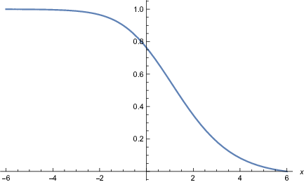
In Figure 2 below, we plot $h(x)=\mathbb{P}_{x}\{M_{\tau_{a}}\leq K\}$ by numerically solving the integral equation (3.2) using Mathematica.

5 Acknowledgments

The authors would like to thank two anonymous referees for their helpful comments and suggestions. Support from grants from the Natural Sciences and Engineering Research Council of Canada is gratefully acknowledged by David Landriault and Bin Li (grant numbers 341316 and 05828, respectively). Support from a start-up grant from the University of Waterloo is gratefully acknowledged by Bin Li, as is support from the Canada Research Chair Program by David Landriault.

Appendix A Appendix

A.1 Proof of Lemma 2.1

We define $\psi_{n}(z)=\inf_{m\geq n}\phi_{m}(z)$ for $z\in S$ . Further, we define $\underline{\psi}_{n}(z)=\liminf_{w\rightarrow z}\psi_{n}(w)$ which is lower semi-continuous (see, e.g., Lemma 5.13.4 of Berberian [6]). Note that $\underline{\psi}_{n}$ is increasing in $n$ , and by the definition of $\underline{\psi}_{n}$ , we have

	$\displaystyle\lim_{n\rightarrow\infty}\underline{\psi}_{n}(z)=$	$\displaystyle\lim_{n\rightarrow\infty}\lim_{r\downarrow 0}\inf_{w\in(z-r,z+r)}\inf_{m\geq n}\phi_{m}(w)$
	$\displaystyle=$	$\displaystyle\lim_{n\rightarrow\infty}\lim_{r\downarrow 0}\inf_{m\geq n,w\in(z-r,z+r)}\phi_{m}(w)\equiv\liminf_{n\rightarrow\infty,w\rightarrow z}\phi_{n}(w),$

where the second equality is because there is no ambiguity in switching the order of two infimums. By the monotone convergence theorem, we have

\int_{S}\liminf_{n\rightarrow\infty,w\rightarrow z}\phi_{n}(w)\mathrm{d}\mu(z)=\lim_{n\rightarrow\infty}\int_{S}\underline{\psi}_{n}(z)\mathrm{d}\mu(z).

(A.1)

By Portmanteau theorem of weak convergence and the fact that $\underline{\psi}_{n}(z)$ is nonnegative and lower semi-continuous, it follows that

\int_{S}\underline{\psi}_{n}(z)\mathrm{d}\mu(z)\leq\liminf_{m\rightarrow\infty}\int_{S}\underline{\psi}_{n}(z)\mathrm{d}\mu_{m}(z)

(A.2)

for any $n\in\mathbb{N}$ . Moreover, since $\psi_{n}(z)$ is monotone increasing in $n$ , we have

\liminf_{m\rightarrow\infty}\int_{S}\underline{\psi}_{n}(z)\mathrm{d}\mu_{m}(z)\leq\liminf_{m\rightarrow\infty}\int_{S}\underline{\psi}_{m}(z)\mathrm{d}\mu_{m}(z).

(A.3)

By (A.1)-(A.3),

\int_{S}\liminf_{n\rightarrow\infty,w\rightarrow z}\phi_{n}(w)\mathrm{d}\mu(z)\leq\liminf_{m\rightarrow\infty}\int_{S}\underline{\psi}_{m}(z)\mathrm{d}\mu_{m}(z)\leq\liminf_{m\rightarrow\infty}\int_{S}\phi_{m}(z)\mathrm{d}\mu_{m}(z),

where the last inequality is due to $\underline{\psi}_{m}(z)\leq\psi_{m}(z)\leq\phi_{m}(z)$ .

Suppose that $\{\phi_{n}\}_{n\in\mathbb{N}}$ is uniformly bounded by $K>0$ , by applying (2.7) to $\{K-\phi_{n}\}_{n\in\mathbb{N}}$ , we obtain

	$\displaystyle K\mu(S)-\int_{S}\limsup_{n\rightarrow\infty,w\rightarrow z}\phi_{n}(w)\mathrm{d}\mu(z)$	$\displaystyle=\int_{S}\liminf_{n\rightarrow\infty,w\rightarrow z}(K-\phi_{n}(w))\mathrm{d}\mu(z)$
		$\displaystyle\leq\liminf_{n\rightarrow\infty}\int_{S}(K-\phi_{n}(z))\mathrm{d}\mu_{n}(z)$
		$\displaystyle=K\liminf_{n\rightarrow\infty}\mu_{n}(S)-\limsup_{n\rightarrow\infty}\int_{S}\phi_{n}(z)\mathrm{d}\mu_{n}(z).$

Therefore, inequality (2.8) follows immediately by the weak convergence of $\mu_{n}$ and $\mu(S)<\infty$ .

A.2 Assumption verification for Example 3.4

Lemma A.1

Consider the PMEP (3.12) with a continuous jump size distribution $F(\cdot)$ . For $q,s\geq 0$ and $0<u_{0}<x_{0}<v_{0}$ , we have

\lim_{(u,v)\downarrow(u_{0},v_{0})}g(x_{0};u,v)=\lim_{(x,u)\uparrow(x_{0},u_{0})}g(x;u,v_{0})=g(x_{0},u_{0},v_{0}),

where the function $g(x;u,v)$ is any of the following three functions: $B_{1}^{(q)}(x;u,v)$ , $B_{2}^{(q,s)}(x;u,v)$ and $C^{(q,s)}(x;u,v)$ .

Proof. Note that the condition $0<u_{0}<x_{0}<v_{0}$ is to ensure the process $X$ remains positive before exiting these finite intervals, which further implies $X$ is upward regular and creeps upward. We limit our proof to

\lim_{(u,v)\downarrow(u_{0},v_{0})}B_{1}^{(q)}(x_{0};u,v)=B_{1}^{(q)}(x_{0};u_{0},v_{0}).

(A.4)

The other results can be proved in a similar manner. By the relationship $v>v_{0}>u>u_{0}$ , we have

		$\displaystyle\left\|B_{1}^{(q)}(x_{0};u_{0},v_{0})-B_{1}^{(q)}(x_{0};u,v)\right\|$
		$\displaystyle\leq\left\|\mathbb{E}_{x_{0}}\left[e^{-qT_{v_{0}}^{+}}1_{\{T_{v_{0}}^{+}<T_{u_{0}}^{-},X_{T_{v_{0}}^{+}}=v_{0}\}}\right]-\mathbb{E}_{x_{0}}\left[e^{-qT_{v}^{+}}1_{\{T_{v}^{+}<T_{u}^{-},X_{T_{v}^{+}}=v,X_{T_{v_{0}}^{+}}=v_{0}\}}\right]\right\|$
		$\displaystyle+\mathbb{P}_{x_{0}}\left\{v_{0}<X_{T_{v_{0}}^{+}}\leq v\right\}.$		(A.5)

It is clear that the last term of (A.5) vanishes as $v\downarrow v_{0}$ by the right-continuity of the distribution function of $X_{T_{v_{0}}^{+}}$ . Also,

		$\displaystyle\left\|\mathbb{E}_{x_{0}}\left[e^{-qT_{v_{0}}^{+}}1_{\{T_{v_{0}}^{+}<T_{u_{0}}^{-},X_{T_{v_{0}}^{+}}=v_{0}\}}\right]-\mathbb{E}_{x_{0}}\left[e^{-qT_{v}^{+}}1_{\{T_{v}^{+}<T_{u}^{-},X_{T_{v}^{+}}=v,X_{T_{v_{0}}^{+}}=v_{0}\}}\right]\right\|$
		$\displaystyle=\mathbb{E}_{x_{0}}\left[e^{-qT_{v_{0}}^{+}}1_{\{T_{v_{0}}^{+}<T_{u}^{-},X_{T_{v_{0}}^{+}}=v_{0}\}}\right]-\mathbb{E}_{x_{0}}\left[e^{-qT_{v}^{+}}1_{\{T_{v}^{+}<T_{u}^{-},X_{T_{v}^{+}}=v,X_{T_{v_{0}}^{+}}=v_{0}\}}\right]$
		$\displaystyle+\mathbb{E}_{x_{0}}\left[e^{-qT_{v_{0}}^{+}}1_{\{T_{u}^{-}<T_{v_{0}}^{+}<T_{u_{0}}^{-},X_{T_{v_{0}}^{+}}=v_{0}\}}\right]$
		$\displaystyle\leq 1-\mathbb{E}_{v_{0}}\left[e^{-qT_{v}^{+}}1_{\{T_{v}^{+}<T_{u}^{-},X_{T_{v}^{+}}=v\}}\right]+\mathbb{P}_{x_{0}}\left\{T_{u}^{-}<T_{v_{0}}^{+}<T_{u_{0}}^{-}\right\}.$		(A.6)

Let $\zeta$ be the time of the first jump of the compound Poisson process $Z$ with jump rate $\lambda>0$ . Note that $X$ will increase continuously up to time $\zeta$ as long as the initial value is positive. Since $v>v_{0}>0$ , we have

1-\mathbb{E}_{v_{0}}\left[e^{-qT_{v}^{+}}1_{\{T_{v}^{+}<T_{u}^{-},X_{T_{v}^{+}}=v\}}\right]\leq 1-\mathbb{E}_{v_{0}}\left[e^{-qT_{v}^{+}}1_{\{{\color[rgb]{0,0,0}\zeta}>T_{v}^{+}\}}\right]=1-\left(\frac{v}{v_{0}}\right)^{-(q+\lambda)/\mu}.

(A.7)

By conditioning on $X_{T_{u}^{-}-}$ , one obtains

	$\displaystyle\mathbb{P}_{x_{0}}\left\{T_{u}^{-}<T_{v_{0}}^{+}<T_{u_{0}}^{-}\right\}$	$\displaystyle\leq\int_{u}^{v_{0}}\mathbb{P}_{x_{0}}\left\{X_{T_{u}^{-}-}\in\mathrm{d}y\right\}\mathbb{P}\left\{y-u<J\leq y-u_{0}\right\}$
		$\displaystyle\leq\max_{u_{0}\leq y\leq v_{0}}\left(F(y-u_{0})-F(y-u)\right).$		(A.8)

Since $F(\cdot)$ is continuous, and hence uniformly continuous for $y\in[0,v_{0}-u_{0}]$ , it follows that the right-hand side of (A.8) vanishes as $u\downarrow u_{0}$ . From (A.5)–(A.8), we conclude that (A.4) holds.

Note that although (A.8) only uses the continuity of $F$ on $[0,\infty)$ , the proof for $C^{(q,s)}(x;u,v)$ will use the continuity of $F$ on $(-\infty,0]$ .

Proposition A.1

Assumptions (A1)-(A3) hold for the piecewise exponential Markov process (3.12) with a continuous jump size distribution $F(\cdot)$ and initial value $X_{0}\geq a$ .

Proof. For $0<u<x<v$ , by the strong Markov property, we have

	$\displaystyle B_{1}^{(q)}(x;u,v)$	$\displaystyle=\mathbb{E}_{x}\left[e^{-qT_{v}^{+}}1_{\{T_{v}^{+}<T_{u}^{-},X_{T_{v}^{+}}=v,\zeta>T_{v}^{+}\}}\right]+\mathbb{E}_{x}\left[e^{-qT_{v}^{+}}1_{\{T_{v}^{+}<T_{u}^{-},X_{T_{v}^{+}}=v,\zeta<T_{v}^{+}\}}\right]$
		$\displaystyle=\left(\frac{v}{x}\right)^{-(q+\lambda)/\mu}+\lambda\int_{0}^{\frac{1}{\mu}\ln\frac{v}{x}}e^{-(q+\lambda)t}\mathrm{d}t\int_{u-xe^{\mu t}}^{v-xe^{\mu t}}B_{1}^{(q)}(xe^{\mu t}+w;u,v)F(\mathrm{d}w).$		(A.9)

By Lemma A.1, Eq. (A.9), and the dominated convergence theorem, it is straightforward to verify that Assumption (A1) holds and for $x>a$ ,

b_{a,1}^{(q)}(x)=\frac{q+\lambda}{\mu x}-\frac{\lambda}{\mu x}\int_{-a}^{0}B_{1}^{(q)}(x+w;x-a,x)F(\mathrm{d}w).

Note that we require $x>a$ as otherwise $x+w$ in the above equation could be negative for $w\in(-a,0)$ , and then Lemma A.1 does not apply. Obviously, $\int_{x}^{y}b_{a,1}^{(q)}(w)\mathrm{d}w<\infty$ for all $0<x<y<\infty$ . Similarly, by conditioning on the first jump of $Z$ , for $0<u<x<v$ ,

	$\displaystyle B_{2}^{(q)}(x,\mathrm{d}z;u,v)$	$\displaystyle=\lambda\int_{0}^{\frac{1}{\mu}\ln\frac{v}{x}}e^{-(q+\lambda)t}F(v-xe^{\mu t}+\mathrm{d}z)\mathrm{d}t$
		$\displaystyle+\lambda\int_{0}^{\frac{1}{\mu}\ln\frac{v}{x}}e^{-(q+\lambda)t}\mathrm{d}t\int_{u-xe^{\mu t}}^{v-xe^{\mu t}}B_{2}^{(q)}(xe^{\mu t}+w,\mathrm{d}z;u,v)F(\mathrm{d}w),$

and

C^{(q,s)}(x;u,v)=\lambda\int_{0}^{\frac{1}{\mu}\ln\frac{v}{x}}e^{-(q+\lambda)t}\mathrm{d}t\int_{-\infty}^{v-xe^{\mu t}}C^{(q,s)}(xe^{\mu t}+w;u,v)F(\mathrm{d}w),

where it is understood that $C^{(q,s)}(xe^{\mu t}+w;u,v)=e^{s(xe^{\mu t}+w-u)}$ for $w<u-xe^{\mu t}$ . One can verify from Lemma A.1 and the dominated convergence theorem that Assumptions (A2) and (A3) hold, and for $x>a,$

{\color[rgb]{0,0,0}b_{a,2}^{(q)}(x,\mathrm{d}z)}=\frac{\lambda}{\mu x}F(\mathrm{d}z)+\frac{\lambda}{\mu x}\int_{-a}^{0}B_{2}^{(q)}(x+w,\mathrm{d}z;x-a,x)F(\mathrm{d}w),

and

c_{a}^{(q,s)}(x)=\frac{\lambda}{\mu x}\int_{-\infty}^{0}C^{(q,s)}(x+w;x-a,x)F(\mathrm{d}w).

This ends the proof.

A.3 Assumption verification for Example 3.5

Let $U$ be the continuous component of $X$ , which is a linear diffusion process with the infinitesimal generator $\mathcal{L}_{U}=\frac{1}{2}\sigma^{2}(y)\frac{\mathrm{d}^{2}}{\mathrm{d}y^{2}}+\mu(y)\frac{\mathrm{d}}{\mathrm{d}y}.$ It is well-known that, for any $q>0$ , there exist two independent and positive solutions, denoted as $\phi_{q}^{\pm}(y)$ , to the Sturm-Liouville equation

\mathcal{L}_{U}\phi_{q}^{\pm}(y)=q\phi_{q}^{\pm}(y),

(A.10)

where $\phi_{q}^{+}(\cdot)$ is strictly increasing and $\phi_{q}^{-}(\cdot)$ is strictly decreasing. By the Lipschitz assumption on $\mu(\cdot)$ and $\sigma(\cdot)$ , it follows from the Schauder estimates (e.g., Theorem 6.14 of Gilbarg and Trudinger [11]) of Eq. (A.10) that $\phi_{q}^{\pm}(\cdot)\in C^{2,\alpha}(\bar{\Omega})$ for any $\alpha\in(0,1]$ and any compact set $\bar{\Omega}\subset\mathbb{R}$ . Interested readers can refer to Section 4.1 of Gilbarg and Trudinger [11] for more detail on the Hölder space $C^{2,\alpha}(\bar{\Omega})$ .

We denote the first hitting time of $U$ to level $z\in\mathbb{R}$ by $H_{z}=\inf\{t>0:U_{t}=z\}$ . It is well-known that, for $u\leq x\leq v$ ,

\mathbb{E}_{x}\left[e^{-qH_{u}}1_{\left\{H_{u}<H_{v}\right\}}\right]=\frac{f_{q}(x,v)}{f_{q}(u,v)}\quad\text{and\quad}\mathbb{E}_{x}\left[e^{-qH_{v}}1_{\left\{H_{v}<H_{u}\right\}}\right]=\frac{f_{q}(u,x)}{f_{q}(u,v)},

(A.11)

where $f_{q}(x,y):=\phi_{q}^{+}(x)\phi_{q}^{-}(y)-\phi_{q}^{+}(y)\phi_{q}^{-}(x)$ . Note that $f_{q}(x,y)$ is strictly decreasing in $x$ and strictly increasing in $y$ with $f_{q}(x,x)=0$ . In particular, for $u\leq x\leq v$ , we have

\mathbb{E}_{x}\left[{e}^{-qH_{u}}\right]=\frac{\phi_{q}^{-}(x)}{\phi_{q}^{-}(u)}\quad\text{and\quad}\mathbb{E}_{x}\left[{e}^{-qH_{v}}\right]=\frac{\phi_{q}^{+}(x)}{\phi_{q}^{+}(v)}.

(A.12)

For $\mathbf{e}_{q}$ an independent exponential random variable with mean $1/q<\infty$ , the $q$ -potential measure of $U$ is given by

r_{q}(x,y):=\frac{1}{q}\mathbb{P}_{x}\left\{U_{\mathbf{e}_{q}}\in\mathrm{d}y\right\}/\mathrm{d}y=\left\{\begin{array}[c]{l}\frac{2}{q\sigma^{2}(y)}\frac{\phi_{q}^{+}(x)\phi_{q}^{-}(y)}{f_{q,1}(y,y)},\quad x\leq y,\\ \frac{2}{q\sigma^{2}(y)}\frac{\phi_{q}^{+}(y)\phi_{q}^{-}(x)}{f_{q,1}(y,y)},\quad x>y,\end{array}\right.

where $f_{q,1}(x,y):=\frac{\partial}{\partial x}f_{q}(x,y).$ Furthermore, the $q$ -potential measure of $U$ killed on exiting the interval $[u,v]$ , for $u\leq x,y\leq v$ , is given by

	$\displaystyle\theta^{(q)}(x,y;u,v)$	$\displaystyle:=\frac{1}{q}\mathbb{P}_{x}\left(U_{\mathbf{e}_{q}}\in\mathrm{d}y,\mathbf{e}_{q}<H_{u}\wedge H_{v}\right)/\mathrm{d}y$
		$\displaystyle=r_{q}(x,y)-\frac{f_{q}(x,v)}{f_{q}(u,v)}r_{q}(u,y)-\frac{f_{q}(u,x)}{f_{q}(u,v)}r_{q}(v,y).$		(A.13)

The next lemma is an analogy of Lemma A.1. Thanks to the diffusion term in the jump diffusion model (3.13), we now allow for the presence of atoms in the jump intensity measure $\nu(\cdot)$ .

Lemma A.2

Consider the jump diffusion model (3.13). For $q,s\geq 0$ and $u_{0}<x_{0}<v_{0}$ , we have

\lim_{(u,v)\downarrow(u_{0},v_{0})}g(x_{0};u,v)=\lim_{(x,u)\uparrow(x_{0},u_{0})}g(x;u,v_{0})=g(x_{0},u_{0},v_{0}),

where $g(x;u,v)$ is any of the following functions: $B_{1}^{(q)}(x;u,v)$ , $B_{2}^{(q,s)}(x;u,v)$ and $C^{(q,s)}(x;u,v)$ .

Proof. We can follow the same proof as Lemma A.1 except for the term $\mathbb{P}_{x_{0}}\left\{T_{u}^{-}<T_{v_{0}}^{+}<T_{u_{0}}^{-}\right\}$ in (A.8), which will be handled distinctly here. We have $X_{t}=U_{t}$ a.s. for $t<\zeta$ , where $\zeta$ is the first time a jump occurs which follows an exponential distribution with mean $1/\lambda=1/\nu(\mathbb{R})>0$ . For any $u_{0}<u<x_{0}<v_{0}$ , by (A.11) and (A.12), we have

	$\displaystyle\mathbb{P}_{x_{0}}\left\{T_{u}^{-}<T_{v_{0}}^{+}<T_{u_{0}}^{-}\right\}$	$\displaystyle\leq\mathbb{P}_{u}\left\{T_{v_{0}}^{+}<T_{u_{0}}^{-}\right\}$
		$\displaystyle=\mathbb{P}_{u}\left\{T_{v_{0}}^{+}<T_{u_{0}}^{-},\xi>T_{v_{0}}^{+}\right\}+\mathbb{P}_{u}\left\{\xi\leq T_{v_{0}}^{+}<T_{u_{0}}^{-}\right\}$
		$\displaystyle\leq\mathbb{E}_{u}\left[e^{-\lambda H_{v_{0}}}1_{\left\{H_{v_{0}}<H_{u_{0}}\right\}}\right]+1-\mathbb{E}_{u}\left[e^{-\lambda H_{u_{0}}}\right]$
		$\displaystyle=\frac{f_{q}(u_{0},u)}{f_{q}(u_{0},v_{0})}+1-\frac{\phi_{q}^{-}(u)}{\phi_{q}^{-}(u_{0})}.$

Therefore, it follows that $\lim_{u\downarrow u_{0}}\mathbb{P}_{x_{0}}\left\{T_{u}^{-}<T_{v_{0}}^{+}<T_{u_{0}}^{-}\right\}=0$ by $f_{q}(u_{0},u_{0})=0$ .

Proposition A.2

Assumptions (A1)-(A3) hold for the jump diffusion model (3.13).

Proof. By the strong Markov property, (A.11) and (A.13), for $u<x<v$ , it follows that

		$\displaystyle B_{1}^{(q)}(x;u,v)$
		$\displaystyle=\mathbb{E}_{x}\left[e^{-qT_{v}^{+}}1_{\{T_{v}^{+}<T_{u}^{-},T_{v}^{+}=v,\zeta>T_{v}^{+}\}}\right]+\mathbb{E}_{x}\left[e^{-qT_{v}^{+}}1_{\{T_{v}^{+}<T_{u}^{-},T_{v}^{+}=v,\zeta<T_{v}^{+}\}}\right]$
		$\displaystyle=\mathbb{E}_{x}\left[e^{-(q+\lambda)H_{v}}1_{\{H_{v}<H_{u}\}}\right]+\int_{u}^{v}\mathbb{E}_{x}\left[e^{-q\zeta}1_{\{\zeta<H_{u}\wedge H_{v},U_{\zeta}\in\mathrm{d}y\}}\right]\int_{\mathbb{R}}B_{1}^{(q)}(y+\gamma(y,w);u,v)\frac{\nu(\mathrm{d}w)}{\lambda}$
		$\displaystyle=\frac{f_{q+\lambda}(u,x)}{f_{q+\lambda}(u,v)}+\int_{u}^{v}\theta^{(q+\lambda)}(x,y;u,v)\mathrm{d}y\int_{\mathbb{R}}B_{1}^{(q)}(y+\gamma(y,w);u,v)\nu(\mathrm{d}w),$

where it is understood that $B_{1}^{(q)}(y+\gamma(y,w);u,v)=0$ if $\gamma(y,w)>v-y$ or $\gamma(y,w)<u-y$ . By Lemma A.2, the dominated convergence theorem, and the identity $f_{q+\lambda}(u,v)=-f_{q+\lambda}(v,u)$ , we can verify that Assumption (A1) holds with

b_{a,1}^{(q)}(x)=\frac{-f_{q+\lambda,1}(x-a,x)}{f_{q+\lambda}(x-a,x)}-\int_{x-a}^{x}\tilde{\theta}_{a}^{(q+\lambda)}(x,y)\mathrm{d}y\int_{\mathbb{R}}B_{1}^{(q)}(y+\gamma(y,w);x-a,x)\nu(\mathrm{d}w),

where we write $\tilde{\theta}_{a}^{(q+\lambda)}(x,y):=-\frac{f_{q+\lambda,1}(x-a,x)}{f_{q+\lambda}(x-a,x)}r_{q+\lambda}(x,y)-r_{q+\lambda,1}(x,y)+\frac{f_{q+\lambda,1}(x,x)}{f_{q+\lambda}(x-a,x)}r_{q+\lambda}(x-a,y)$ and $r_{q+\lambda,1}(x,y):=\frac{\partial}{\partial x}r_{q+\lambda}(x,y).$ The integrability of $b_{a,1}^{(q)}(\cdot)$ follows from the continuity of the $\phi_{q}^{+}(\cdot)$ and $\phi_{q}^{-}(\cdot)$ .

Similarly, by the strong Markov property of $X$ , (A.11) and (A.13), we have

B_{2}^{(q)}(x,\mathrm{d}z;u,v)=\int_{u}^{v}\theta^{(q+\lambda)}(x,y;u,v)\mathrm{d}y\int_{\mathbb{R}}B_{2}^{(q)}(y+\gamma(y,w),\mathrm{d}z;u,v)\nu(\mathrm{d}w),

and

C^{(q,s)}(x;u,v)=\frac{f_{q+\lambda}(x,v)}{f_{q+\lambda}(u,v)}+\int_{u}^{v}\theta^{(q+\lambda)}(x,y;u,v)\mathrm{d}y\int_{\mathbb{R}}C^{(q,s)}(y+\gamma(y,w);u,v)\nu(\mathrm{d}w).

One can verify from Lemma A.2 that Assumptions (A2) and (A3) hold with

b_{2,a}^{(q)}(x,\mathrm{d}z)=\int_{x-a}^{x}\tilde{\theta}_{a}^{(q+\lambda)}(x,y)\mathrm{d}y\int_{\mathbb{R}}B_{2}^{(q)}(y+\gamma(y,w),\mathrm{d}z;x-a,x)\nu(\mathrm{d}w),

and

c_{a}^{(q,s)}(x)=\frac{-f_{q+\lambda,1}(x,x)}{f_{q+\lambda}(x-a,x)}+\int_{x-a}^{x}\tilde{\theta}^{(q+\lambda)}(x,y)\mathrm{d}y\int_{\mathbb{R}}C^{(q,s)}(y+\gamma(y,z);x-a,x)\nu(\mathrm{d}w).

This completes the proof.

References

[1] Albrecher, H.; Ivanovs, J.; Zhou, X. Exit identities for Lévy processes observed at Poisson arrival times. Bernoulli 22 (2016), no. 3, 1364–1382.
[2] Asmussen, S.; Avram, F.; Pistorius, M. R. Russian and American put options under exponential phase-type Lévy models. Stochastic Process. Appl. 109 (2004), no. 1, 79–111.
[3] Avram, F.; Kyprianou, A. E.; Pistorius, M. R. Exit problems for spectrally negative Lévy processes and applications to (Canadized) Russian options. Ann. Appl. Probab. 14 (2004), no. 1, 215–238.
[4] Avram, F.; Palmowski, Z.; Pistorius, M. R. On the optimal dividend problem for a spectrally negative Lévy process. Ann. Appl. Probab. 17 (2007), no. 1, 156–180.
[5] Baurdoux, E. J. Some excursion calculations for reflected Lévy processes. ALEA Lat. Am. J. Probab. Math. Stat. 6 (2009), 149–162.
[6] Berberian, S. K. Fundamentals of Real Analysis, Springer-Verlag, New York, 1999.
[7] Carr, P.; Zhang, H.; Hadjiliadis, O. Maximum drawdown insurance. Int. J. Theor. Appl. Finance 14 (2011), no. 8, 1195–1230.
[8] Cherny, V.; Obloj, J. Portfolio optimisation under non-linear drawdown constraints in a semimartingale financial model. Finance Stoch. 17 (2013), no. 4, 771–800.
[9] Douady, R.; Shiryaev, A. N.; Yor, M. On probability characteristics of ”downfalls” in a standard Brownian motion. Theory Probab. Appl. 44 (2000), no. 1, 29–38.
[10] Feinberg, E. A.; Kasyanov, P. O.; Zadoianchuk N. V. Fatou’s Lemma for weakly converging probabilities. Theory Probab. Appl. 4 (2014), no. 58, 683–689.
[11] Gilbarg, D.; Trudinger, N. S. Elliptic partial differential equations of second order. Reprint of the 1998 edition. Springer-Verlag, Berlin, 2001.
[12] Gjessing, H. K.; Paulsen, J. Present value distributions with applications to ruin theory and stochastic equations. Stochastic Process. Appl. 71 (1997), no. 1, 123–144.
[13] Grossman, S. J.; Zhou, Z. Optimal investment strategies for controlling drawdowns, Math. Finance 3 (1993), no. 3, 241–276.
[14] Ivanovs, J.; Palmowski, Z. Occupation densities in solving exit problems for Markov additive processes and their reflections. Stochastic Process. Appl. 122 (2012), no. 9, 3342–3360.
[15] Jacobsen, M.; Jensen, A. T. Exit times for a class of piecewise exponential Markov processes with two-sided jumps. Stochastic Process. Appl. 117 (2007), no. 9, 1330–1356.
[16] Kallenberg, O. Foundations of modern probability. Second edition. Probability and its Applications. Springer-Verlag, New York, 2002.
[17] Kella, O.; Stadje, W. On hitting times for compound Poisson dams with exponential jumps and linear release rate. J. Appl. Probab. 38 (2001), no. 3, 781–786.
[18] Kuznetsov, A.; Kyprianou, A. E.; Rivero, V. The theory of scale functions for spectrally negative Lévy processes. Lévy matters II, 97–186, Lecture Notes in Math., 2061, Springer, Heidelberg, 2012.
[19] Kyprianou, A. E. Fluctuations of Lévy processes with applications. Second edition. Springer, Heidelberg, 2014.
[20] Kyprianou, A. E.; Loeffen, R. L. Refracted Lévy processes. Ann. Inst. Henri Poincaré Probab. Stat. 46 (2010), no. 1, 24–44.
[21] Kyprianou, A. E.; Palmowski, Z. Distributional study of de Finetti’s dividend problem for a general Lévy insurance risk process. J. Appl. Probab. 44 (2007), no. 2, 428–443.
[22] Kyprianou, A. E.; Zhou, X. General tax structures and the Lévy insurance risk model. J. Appl. Probab. 46 (2009), no. 4, 1146–1156.
[23] Landriault, D.; Li, B.; Zhang, H. On magnitude, asymptotics and duration of drawdowns for Lévy models. Bernoulli (2016), forthcoming.
[24] Lehoczky, J. P. Formulas for stopped diffusion processes with stopping times based on the maximum. Ann. Probability 5 (1977), no. 4, 601–607.
[25] Li, B.; Tang, Q.; Zhou, X. A time-homogeneous diffusion model with tax. J. Appl. Probab. 50 (2013), no. 1, 195–207.
[26] Loeffen, R. L. On optimality of the barrier strategy in de Finetti’s dividend problem for spectrally negative Lévy processes. Ann. Appl. Probab. 18 (2008), no. 5, 1669–1680.
[27] Magdon-Ismail, M.; Atiya, A. F.; Pratap, A.; Abu-Mostafa, Y. On the maximum drawdown of a Brownian motion. J. Appl. Probab. 41 (2004), no. 1, 147–161.
[28] Mijatovic, A.; Pistorius, M. R. On the drawdown of completely asymmetric Lévy processes. Stochastic Process. Appl. 122 (2012), no. 11, 3812–3836.
[29] Øksendal, B.; Sulem, A. Applied stochastic control of jump diffusions. Second edition. Universitext. Springer, Berlin, 2007.
[30] Pistorius, M. R. On exit and ergodicity of the spectrally one-sided Lévy process reflected at its infimum. J. Theoret. Probab. 17 (2004), no. 1, 183–220.
[31] Poor, H. V.; Hadjiliadis, O. Quickest detection. Cambridge University Press, Cambridge, 2009.
[32] Pospisil, L.; Vecer, J.; Hadjiliadis, O. Formulas for stopped diffusion processes with stopping times based on drawdowns and drawups. Stochastic Process. Appl. 119 (2009), no. 8, 2563–2578.
[33] Rogers, L. C. G.; Williams, D. Diffusions, Markov processes, and martingales: volume 1, foundations. Second edition. Cambridge University Press, Cambridge, 2000.
[34] Schuhmacher, F.; Eling, M. Sufficient conditions for expected utility to imply drawdown-based performance rankings. Journal of Banking & Finance 35 (2011), 2311–2318.
[35] Shepp, L.; Shiryaev, A. N. The Russian option: reduced regret. Ann. Appl. Probab. 3 (1993), no. 3, 631–640.
[36] Taylor, H. M. A stopped Brownian motion formula. Ann. Probab. 3 (1975), 234–246.
[37] Tsurui, A.; Osaki, S. On a first-passage problem for a cumulative process with exponential decay. Stochastic Processes Appl. 4 (1976), no. 1, 79–88.
[38] Widder, D. V. The Laplace Transform. Princeton University Press, 1946.
[39] Yuen, K. C.; Wang, G.; Ng, K. W. Ruin probabilities for a risk process with stochastic return on investments. Stochastic Process. Appl. 110 (2004), no. 2, 259–274.
[40] Zhang, H. Occupation time, drawdowns, and drawups for one-dimensional regular diffusion. Adv. in Appl. Probab. 47 (2015), no. 1, 210–230.
[41] Zhang, H.; Hadjiliadis, O. Drawdowns and rallies in a finite time-horizon. Drawdowns and rallies. Methodol. Comput. Appl. Probab. 12 (2010), no. 2, 293–308.
[42] Zhang, H.; Leung, T.; Hadjiliadis, O. Stochastic modeling and fair valuation of drawdown insurance. Insurance Math. Econom. 53 (2013), no. 3, 840–850.
[43] Zhou, X. Exit problems for spectrally negative Lévy processes reflected at either the supremum or the infimum. J. Appl. Probab. 44 (2007), no. 4, 1012–1030.