VaST: a variability search toolkit^⋆

Journal: Astronomy & Computing

Kirill V. Sokolovsky Address: IAASARS, National Observatory of Athens, Vas. Pavlou & I. Metaxa, 15236 Penteli, Greece; email: kirx@noa.gr Address: Sternberg Astronomical Institute, Moscow State University, Universitetskii pr. 13, 119992 Moscow, Russia Address: Astro Space Center, Lebedev Physical Institute, Russian Academy of Sciences, Profsoyuznaya St. 84/32, 117997 Moscow, Russia Alexandr A. Lebedev Address: Yandex School of Data Analysis, Timura Frunze St. 11/2, 119021 Moscow, Russia

Abstract

Variability Search Toolkit (VaST) is a software package designed to find variable objects in a series of sky images. It can be run from a script or interactively using its graphical interface. VaST relies on source list matching as opposed to image subtraction. SExtractor is used to generate source lists and perform aperture or PSF-fitting photometry (with PSFEx). Variability indices that characterize scatter and smoothness of a lightcurve are computed for all objects. Candidate variables are identified as objects having high variability index values compared to other objects of similar brightness. The two distinguishing features of VaST are its ability to perform accurate aperture photometry of images obtained with non-linear detectors and handle complex image distortions. The software has been successfully applied to images obtained with telescopes ranging from 0.08 to 2.5 m in diameter equipped with a variety of detectors including CCD, CMOS, MIC and photographic plates. About 1800 variable stars have been discovered with VaST. It is used as a transient detection engine in the New Milky Way (NMW) nova patrol. The code is written in C and can be easily compiled on the majority of UNIX-like systems. VaST is free software available at http://scan.sai.msu.ru/vast/

Keywords:

methods: data analysis , techniques: photometric , stars: variables

1 Introduction

^$\star$^$\star$footnotetext: This code is registered at the ASCL with the code entry ascl:1704.005.

Variable stars are important tracers of stellar evolution (Sherwood and Plaut 1975, e.g.), fundamental stellar parameters (Torres et al. 2010), 3D structure of our Galaxy (Pietrukowicz et al. 2015, Dékány et al. 2015, Gran et al. 2016) and beyond (Lah et al. 2005, Subramanian and Subramaniam 2012, Hoffmann and Macri 2015, Jacyszyn-Dobrzeniecka et al. 2017) as well as various astrophysical processes related to accretion (Osaki 1996, Mukai 2017), ejection (Russell et al. 2016) and strong magnetic fields (Cropper et al. 1989). It is believed that only a few per cent of the variable stars easily accessible to ground-based photometry are currently known (Samus and Antipin 2015). The reason is that contemporary CCDs are very sensitive and small and hence image only a small field of view to a high limiting magnitude.

The next generation surveys Gaia (Gaia Collaboration et al. 2016, Clementini et al. 2016), VVV (Minniti et al. 2010), Pan-STARRS (Chambers et al. 2016), LSST (Ridgway et al. 2014), NGTS (Wheatley et al. 2017) and TESS (Ricker et al. 2015) employing large mosaic cameras (or multiple small cameras in case of NGTS and TESS) are expected to greatly increase the number of known variable stars. Still, these surveys have their limitations in terms of observing cadence, sky coverage, accessible magnitude range and survey lifetime. All this leaves room for variability searches with other instruments and different observing strategies. Photometric measurements needed to detect stellar variability are relatively easy to perform (compared to spectroscopy and polarimetry of objects with the same brightness), so even small-aperture telescopes are useful for finding and studying variable stars.

Large time-domain surveys employ custom-built pipelines (Bertin et al. 2002, Laher et al. 2014, Kessler et al. 2015, Mauro et al. 2015, e.g.) to perform photometric data reduction and variable object detection. These pipelines are fine-tuned for the particular equipment and observing strategies employed by these surveys and, while often sharing many common pieces of code, require intervention of a software engineer to adopt them to another telescope or camera. Developing a purpose-built pipeline for a small observing project is often impractical. Instead, one would like to have data reduction software applicable to a variety of telescopes and cameras.

The problem of extracting variability information from surveys, in practice, has not been completely solved. New variable stars are still being identified in the NSVS survey data (Khruslov 2013, Sergey et al. 2014, e.g.) while its observations were completed in 1999–2000 (Woźniak et al. 2004). A number of recent ground-based exoplanet transit surveys, despite having sufficient photometric accuracy and sky coverage for detecting the majority of bright variable stars, have so far provided only limited information on individual objects (Rodriguez et al. 2013, Norton et al. 2016, e.g.) or specific classes of objects (Devor et al. 2008, Norton et al. 2011, McQuillin et al. 2012, Holdsworth et al. 2014, Labadie-Bartz et al. 2016, e.g.). Better variability detection algorithms, open data-sharing policies and interfaces to published time-series that allow non-trivial searches in the whole database rather than providing access to a limited number of objects at a time are needed to fully exploit the information hidden in the data. A software to perform variability search in a set of lightcurves imported from a survey archive and visualize the search results may be useful for information extraction and debugging fully-automated search procedures.

Photographic plates used to be the primary type of light detectors in astronomy in the 20th century. Direct images of the sky recorded on glass plates contain information about the positions and brightness that celestial objects had decades ago. This information may be useful on its own or as the first-epoch for comparison with modern CCD measurements. The plates are stored in archives in observatories around the world. Many observatories are digitizing their collections in an effort to preserve the information stored on the plates and make it more accessible. At the time of writing, only the DASCH¹¹ 1 http://dasch.rc.fas.harvard.edu/ (Grindlay et al. 2012) and APPLAUSE²² 2 https://www.plate-archive.org (Groote et al. 2014, Tuvikene et al. 2014) archives provide source catalogs and photometry derived from the plates while others³³ 3 http://dc.zah.uni-heidelberg.de/lswscans/res/positions/q/info^,⁴⁴ 4 http://plate-archive.hs.uni-hamburg.de/index.php/en/ provide only images. Performing photometry on digitized photographic images is a non-trivial task (Bacher et al. 2005, Tang et al. 2013, Wertz et al. 2016) that cannot be done well with conventional photometry software developed for CCD images. The conventional software relies on the assumption that an image sensor responds linearly to the number of incoming photons. This assumption is violated for photographic emulsion as well as for some types of contemporary light detectors including microchannel plate intensified CCDs (MICs) used in space-based UV-sensitive telescopes Swift/UVOT (Poole et al. 2008, Breeveld et al. 2010, see also Brown et al. 2014), XMM/OM (Mason et al. 2001) and fast ground-based cameras (Karpov et al. 2012). There is a need for a user-level software capable of performing photometry on images obtained with non-linear detectors.

A number of software packages for detection of variable objects have been developed recently. Some of them feature a graphical user interface (GUI) and are aimed at processing small datasets, while others have command-line interfaces and are meant as a complete data processing pipeline or as building blocks for constructing one. LEMON⁵⁵ 5 https://github.com/vterron/lemon is a pipeline based on SExtractor⁶⁶ 6 http://www.astromatic.net/software/sextractor (Bertin and Arnouts 1996) and PyRAF for automated time-series reduction and analysis (Terrón and Fernández 2011). It takes a series of FITS images as an input and constructs lightcurves of all objects. PP⁷⁷ 7 https://github.com/mommermi/photometrypipeline (Mommert 2017) is an automated Python pipeline based on SExtractor and SCAMP (Bertin 2006). PP produces calibrated photometry from imaging data with minimal human interaction. While originally designed for asteroid work, the code is be applicable for stellar photometry. LEMON and PP are very similar to VaST in spirit, while they differ in technical implementation and user interface. C-Munipack/Muniwin⁸⁸ 8 http://c-munipack.sourceforge.net/ offers a complete solution for reducing observations of variable stars obtained with a CCD or DSLR camera. It runs on Windows and Linux and provides an intuitive GUI. FotoDif⁹⁹ 9 http://www.astrosurf.com/orodeno/fotodif/ is a Windows CCD photometry package providing capabilities similar to Muniwin. Astrokit¹⁰¹⁰ 10 http://astro.ins.urfu.ru/en/node/1330 (Burdanov et al. 2014, Burdanov et al. 2016) corrects for atmospheric transparency variations by selecting an optimal set of comparison stars for each object in the field. IRAF’s¹¹¹¹ 11 http://iraf.noao.edu/ (Tody 1986) PHOT/APPHOT task is meant to be used to generate input photometric data for Astrokit. Variable star candidates are selected in Astrokit with Robust Median Statistics (Rose and Hintz 2007). FITSH¹²¹² 12 https://fitsh.net/ (Pál 2012) is a collection of tasks for advanced image manipulation (including stacking) and lightcurve extraction using aperture, image subtraction, analytic profile modeling and PSF-fitting photometry. VARTOOLS¹³¹³ 13 http://www.astro.princeton.edu/~jhartman/vartools.html (Hartman and Bakos 2016) implements in C a collection of advanced lightcurve analysis methods providing a command-line interface to them. HOTPANTS¹⁴¹⁴ 14 http://www.astro.washington.edu/users/becker/v2.0/hotpants.html (Becker 2015) is designed to photometrically align one input image with another, after they have been astrometrically aligned with software like WCSremap¹⁵¹⁵ 15 http://www.astro.washington.edu/users/becker/v2.0/wcsremap.html, SWarp (Bertin et al. 2002) or Montage (Jacob et al. 2010). HOTPANTS is an implementation of the Alard (2000) algorithm for image subtraction. The program is intended as a part of a transient detection/photometry pipeline. ISIS¹⁶¹⁶ 16 http://www2.iap.fr/users/alard/package.html (Alard and Lupton 1998) is a complete package to process CCD images using the image subtraction method. It finds variable objects in the subtracted images and builds their light curves from a series of CCD images. DIAPL¹⁷¹⁷ 17 http://users.camk.edu.pl/pych/DIAPL/index.html (Rozyczka et al. 2017) is able to identify variable stars via image subtraction, implemented in C. TraP¹⁸¹⁸ 18 https://github.com/transientskp/tkp (Swinbank et al. 2015) is a Python and SQL based pipeline for detecting transient and variable sources in a stream of astronomical images. It primarily targets LOFAR radio astronomy data, but is also applicable to a range of other instruments (including optical ones).

Most of the above packages were not available at the time VaST development was started (Sokolovsky and Lebedev 2005). Many of them cannot construct lightcurves without finding a plate solution with respect to an external star catalog. None of the above software addresses the issue of photometry with non-linear imaging detectors. VaST provides a combination of features not yet offered by other software, including the ability to process thousands of images with tens of thousands of stars and interactively display the results in a GUI.

VaST is designed as a user-friendly software implementing the full cycle of photometric reduction from calibrating images to producing lightcurves of all objects within a field of view and detecting variable ones. VaST is capable of handling images obtained with non-linear detectors such as photographic plates and MICs. The software may be applied to images obtained with telescopes of any size with minimal configuration. VaST can be used interactively to inspect a set of images of one field in a PGPLOT¹⁹¹⁹ 19 http://www.astro.caltech.edu/~tjp/pgplot/-based GUI. As soon as optimal source extraction and lightcurve post-processing parameters have been identified in the interactive mode, VaST may proceed non-interactively and produce lightcurves for subsequent variability searches with VARTOOLS or custom-built scripts. VaST lightcurve visualization tools and built-in variability statistics routines may also be used to inspect and process lightcurves obtained with other software.

The outline of the paper is as follows. Section 2 presents the overall design of the program centered around the idea of distinguishing variable stars from non-variable ones using “variability indices”. Section 3 describes the steps performed by VaST when processing a set of images. Section 4 presents a specialized transient detection mode that does not rely on variability indices. In Section 5 we present some general remarks on the VaST development procedures. Section 6 gives an account of several notable examples of applying VaST to real data processing. We present a summary in Section 7. A describes common use cases that can be solved with VaST. B presents the list of the command-line arguments to be used with the main program of the toolkit. C describes the log files that summarize image processing results.

2 VaST design and the challenge of variability detection

VaST is designed to accomplish three main tasks:

1.

Construct lightcurves of all objects visible at the input series of images of a given star field.
2.

Compute variability indices to quantify “how variable” each lightcurve appears to be.
3.

Visualize the variability indices, lightcurves and images to let the user decide which objects are actually variable.

In addition, VaST includes tools to calibrate the magnitude zero-point of the produced lightcurves, check if a given object is a cataloged variable, apply the heliocentric correction to a lightcurve, etc. The software modules implementing each of the above tasks are united by a common internal lightcurve file format. They can be run together or independently of each other. All data processing is done within the VaST working directory which contains all the necessary binaries and scripts, so the modules can locate each other without the need to set environment variables. This also allows for an easy “unpack and compile” installation procedure described in A.1.

The input to VaST may be either a set of images (for a practical example see A.2) or a set of lightcurves constructed using other software or imported from an archive (A.14). The output is a set of lightcurves and variability indices computed for each lightcurve. The indices and lightcurves can be either visualized and searched for variable objects interactively or exported for further processing with external software.

The fundamental problem in optical variability detection is that the accuracy of photometric measurements is not precisely known as the measurements may be affected by various systematic effects or corrupted. These effects include, but are not limited to:

1.

Residual sensitivity variations across the detector that were not taken out by flat fielding. These may be both large- (vignetting, defocused images of dust grains in optical path) and small-scale (individual dead pixels). The object’s image moves across the detector due to imperfect guiding resulting in apparent variations in brightness.
2.

Variation of atmospheric extinction across the field.
3.

Differential extinction in the atmosphere resulting in apparent change (as a function of airmass) in relative brightness of stars having different colors.
4.

Charge transfer inefficiency in a CCD (Israel et al. 2015).
5.

Changing seeing conditions resulting in varying degree of overlap between images of nearby objects.
6.

If the instrument’s point spread function (PSF) is not point-symmetric (for example it may have diffraction spikes) the amount of blending between objects will change with changing parallactic angle.
7.

The PSF shape varies across the image resulting in different fraction of object’s light falling within the aperture (in the case of aperture photometry) or presenting a challenge of accurate PSF variations reconstruction (in PSF-fitting photometry).
8.

Resampling and stacking images may also have the unintended consequence of distorting brightness of some sources.

The solution adopted by the community is to rely on the assumption that no instrumental effect can in practice mimic a reasonably well sampled lightcurve of a variable star of a known type. While this is a reasonable assumption for periodic variables, for irregular ones it is necessary to have an idea of the practical limits of the amplitude and timescale of instrumental effects that may be found in a given photometric dataset.

In order to distinguish candidate variables from noise in the absence of reliable estimates of measurement errors one may assume that the majority of stars are not variable at the few per cent level of photometric accuracy (Howell 2008, Sokolovsky et al. 2014a) typically achieved in ground-based survey observations. Using this assumption one may select as candidate variables the objects that appear “more variable” than the majority of objects in this dataset. Among these candidates there will be true variable objects as well as false candidates whose measurements were severely corrupted by some rare instrumental effect like an object’s image falling on a dead pixel. If the instrumental effect is not rare, e.g. if bad pixels are abundant and affect measurements of many stars, the affected stars will not stand out as “more variable” compared to the other stars in the dataset. It is ultimately up to a human expert to investigate lightcurves and images of the candidate variables and judge if the measurements of a particular object are trustworthy or have obvious problems (bad pixels, blending, etc) making them unreliable.

There is a number of ways to characterize a “degree of variability” in a lightcurve. We call the variability indices all the values that:

1.

Quantify the scatter of brightness measurements: $\sigma$ , MAD, IQR, etc. (Ferreira Lopes and Cross 2017, Sokolovsky et al. 2017).
2.

Quantify the smoothness of the lightcurve like the $I$ index (Welch and Stetson 1993) or $1/\eta$ (von Neumann 1941).
3.

Sensitive to both smoothness and scatter (Stetson’s $J$ index), maybe also taking into account the shape of the measured brightness distribution (Stetson 1996, Ferreira Lopes and Cross 2016, e.g. $L$ index).
4.

Characterize the strength of a periodic signal in the lightcurve (Fruth et al. 2012, Sokolovsky et al. 2016, e.g.).

In the absence of detailed information about measurement errors and instrumental effects one should consider the above parameters computed for a given lightcurve in the context of other lightcurves in this dataset to decide if a given variability index value corresponds to a variable object or not. The indices are not equally sensitive to all types of variability. Some of them are more susceptible to individual outliers (corrupted measurements) than the others. Scatter-based indices are generally sensitive to variability of any kind while the indices that characterize smoothness are more sensitive than scatter-based indices to objects that vary slowly compared to the typical observing cadence. That comes at the cost of these indices being insensitive to variability on timescales shorter than the observing cadence. Table 1 presents the list of variability indices computed by VaST. We refer to Sokolovsky et al. (2017) for a detailed discussion and comparison of these indices.

In the following Section we present a detailed description of all the processing steps from reading input images to constructing lightcurves, computing and visualizing the variability indices. A gives practical examples of using the code.

Table 1: Variability indices computed by VaST.

Indices quantifying lightcurve scatter
Index	Reference
weighted std. deviation – $\sigma$	Kolesnikova et al. (2008)
clipped $\sigma$ – $\sigma_{\rm clip}$	Kolesnikova et al. (2008)
median abs. deviation – ${\rm MAD}$	Zhang et al. (2016)
interquartile range – ${\rm IQR}$	Sokolovsky et al. (2017)
reduced $\chi^{2}$ statistic – $\chi_{\rm red}^{2}$	de Diego (2010)
robust median stat. – ${\rm RoMS}$	Rose and Hintz (2007)
norm. excess variance – $\sigma_{\rm NXS}^{2}$	Nandra et al. (1997)
norm. peak-to-peak amp. – $v$	Sokolovsky et al. (2009)
Indices quantifying lightcurve smoothness
autocorrelation – $l_{1}$	Kim et al. (2011)
inv. von Neumann ratio – $1/\eta$	Shin et al. (2009)
Welch–Stetson index – $I_{\rm WS}$	Welch and Stetson (1993)
flux-independent index – $I_{\rm fi}$	Ferreira Lopes et al. (2015)
Stetson’s $J$ index	Stetson (1996)
time-weighted Stetson’s $J_{\rm time}$	Fruth et al. (2012)
clipped Stetson’s $J_{\rm clip}$	Sokolovsky et al. (2017)
Stetson’s $L$ index	Stetson (1996)
time-weighted Stetson’s $L_{\rm time}$	Fruth et al. (2012)
clipped Stetson’s $L_{\rm clip}$	Sokolovsky et al. (2017)
consec. same-sign dev. – Con.	Wozniak (2000)
$S_{B}$ statistic	Figuera Jaimes et al. (2013)
excursions – $E_{x}$	Parks et al. (2014)
excess Abbe value – $\mathcal{E}_{\mathcal{A}}$	Mowlavi (2014)
Indices quantifying magnitude distribution shape
Stetson’s $K$ index	Stetson (1996)
kurtosis	Friedrich et al. (1997)
skewness	Friedrich et al. (1997)

3 Data processing flow

The primary input for VaST is a series of FITS²⁰²⁰ 20 http://fits.gsfc.nasa.gov/ images. The images are expected to be taken with the same telescope-camera-filter combination and cover the same area of the sky. The images may be shifted, rotated and reflected with respect to each other, but should overlap by at least 40 per cent with the sky area covered by the first image. The first image supplied to VaST serves as the astrometric and photometric reference. If the input images vary in quality, it is up to the user to select a good reference image and put it first on the command line (A.3). Below we describe the main processing steps performed to extract lightcurves from a set of images.

3.1 Reading metadata from the FITS header

Information about the observing time, image dimensions and CCD gain information (that is needed to accurately compute contribution of the Poisson/photon noise to the total photometric error), is extracted from FITS header of each input image. The observing time assigned to each image is the middle of the exposure. The exposure start time is derived from one or two (if date and time are given separately) keywords from the following list: DATE-OBS, TIME-OBS, EXPSTART, UT-START, START. The exposure time in seconds is extracted from EXPOSURE or EXPTIME. If none of the two keywords are present in the header, the difference between the observation start and its middle-point is assumed to be negligible (the exposure time is set to 0). The derived time is converted to Julian date (JD).

If no keyword describing the exposure start time is found, but the JD keyword is present in the header, the keyword is assumed to correspond to the middle of exposure. This simplified convention for recording the observation time in the FITS header has been introduced within the program of digitizing photographic plates of Sternberg Astronomical Institute’s collection (Kolesnikova et al. 2008, Kolesnikova et al. 2010, Sokolovsky et al. 2014a). This is different from the definition of the JD keyword adopted by the widely-used CCD camera control software MaxIm DL. However, MaxIm DL will always write the DATE-OBS keyword which, if present, is used by VaST instead of JD. If VaST fails to recognize the format in which the observing time is specified in the FITS header of your images, please send an example image to the authors.

VaST supports the following two time systems: Coordinated Universal Time (UTC) and Terrestrial Time (TT). The Earth rotation period is a few milliseconds longer than 86400 SI seconds and is changing irregularly when measured at this level of accuracy. To keep UTC timescale in sync with the Earth rotation, a leap second is introduced every few years. The UTC time, being the basis of civil time, is readily available in practice through GPS receivers, NTP servers and radio broadcast, so the time of most images is recorded in UTC. The observing time from some instruments, notably Swift/UVOT, is recorded in TT. The advantage of TT is that this timescale is continuous, not interrupted by leap seconds. At each moment of time, the two timescales are related as

{\rm TT}={\rm UTC}+({\rm TAI}-{\rm UTC})+32.184\,{\rm sec}

where $({\rm TAI}-{\rm UTC})$ is the difference between the International Atomic Time (TAI) and UTC for a given date²¹²¹ 21 VaST will automatically get the current $({\rm TAI}-{\rm UTC})$ values from http://maia.usno.navy.mil/ser7/tai-utc.dat. As of spring 2017, the difference between TT and UTC is 69.184 sec.

The program tries to determine the time system in which the observing time is expressed in the FITS header by searching for the TIMESYS key or parsing the comment field for the keyword used to get the time. If neither UTC nor TT are explicitly mentioned in the header, the input time is assumed to be UTC. The observing time in the lightcurves created by VaST is by default expressed in terrestrial time – JD(TT). The conversion from UTC to TT may be disabled (B).

No heliocentric correction is applied to the lightcurves by default, as by design of the program, it is possible to produce lightcurves without knowing the absolute celestial coordinates of the imaged objects. If the coordinates are known, the correction may be applied after constructing a lightcurve as described in A.16. See Eastman et al. (2010) for a detailed discussion of accurate timing problems in the context of optical photometric observations.

3.2 Source extraction and photometry

VaST relies on SExtractor for detecting sources, measuring their positions (in pixel coordinates) and brightness. The source extraction parameters are set in the SExtractor configuration file default.sex located in the VaST directory. Depending on the command-line settings (B), more than one run of SExtractor may be needed for each image:

option I) If all images are to be measured with a circular aperture of the fixed diameter, only a single SExtractor run is performed for each image.

option II) If the circular aperture diameter is allowed to vary between images to account for seeing changes (Collins et al. 2017, e.g.), a preliminary SExtractor run is performed to determine the typical source size. For each source the maximum spatial r.m.s. dispersion of its profile is computed (SExtractor output parameter A_IMAGE). The aperture diameter for each image is computed as $C\times{\rm median(\texttt{A\_IMAGE})}$ , where the median is computed over all the detected sources passing selection criteria and the default value of $C=6.0$ .

option III) If the program is running in the PSF-fitting photometry mode, multiple SExtractor passes over the input image are required. First, a preliminary run is performed to determine seeing, as in the option II) above. Then SExtractor is run with conservative detection limits to extract bright sources and save their small images (SExtractor output parameter VIGNET). These small images are used by PSFEx²²²² 22 http://www.astromatic.net/software/psfex (Bertin 2011) to construct a model of spatially-variable point spread function (PSF). The size of these small images as well as limits on size of objects accepted for PSF reconstruction are determined based on seeing. The PSF reconstruction step is followed by PSF-fitting with SExtractor. Objects that provide a bad fit (non-stellar, heavily blended, corrupted or overexposed objects) are discarded from the output catalog. Finally, an aperture photometry run is conducted with SExtractor (again, same as in option II). This step is performed for technical reasons: a catalog that includes all the objects, even the overexposed ones, is needed at later processing steps to perform absolute astrometric calibration discussed in Section 3.7.

The input images are expected to be well-focused. VaST may be used to process strongly-defocused images with “donut-shaped stars” given a careful selection of the processing parameters including source detection and deblending thresholds (A.8) and manually specified aperture size and star matching radius (Section 3.3, B).

The list of sources detected by SExtractor may be filtered to remove saturated, blended and extended sources as their brightness measurements are less accurate and such sources may appear as spurious candidate variables later in the analysis. Saturated sources are removed based on the source detection flag set by SExtractor. The filtering of blended and extended sources may be accomplished using SExtractor flags (if SExtractor deblending was successful) and by identifying outliers in the magnitude-size plot (Figure 1). The sources that were not properly deblended will appear larger than the other sources of similar brightness. Rejection of blended sources is done using individual images rather than using information about source size and detection flags collected from the full series of images because a generally “good” source may appear blended on some images where it is affected by a cosmic ray hit, a CCD cosmetic defect or a particularly bad seeing. It is desirable to reject only measurements of the source brightness associated with the affected images while keeping the good measurements for further analysis. The acceptable SExtractor flag values (A.8, A.15) and the magnitude-size filter may be controlled using VaST command line options (B).

Refer to caption — Figure 1: Semi-major axis length (SExtractor output parameter A_IMAGE) as a function of instrumental magnitude for sources detected on a CCD frame. Crosses mark sources rejected as being too large for their magnitude (blended or extended).

3.3 Cross-matching source lists

VaST does not require any world coordinate system (WCS; Greisen and Calabretta 2002) information to be present in the headers of the input FITS images. Instead, the code finds a linear transformation of pixel coordinates of objects detected on each image to the pixel coordinate system of the first image (taken as the astrometric reference).²³²³ 23 The use of internal pixel-based coordinate system instead of celestial coordinates may seem strange nowadays, but was natural back in 2004 when we started developing VaST. Before the release of the Astrometry.net software (Lang et al. 2010, Hogg et al. 2008) there was no easy way to assign WCS to “random” images having no a priori information in FITS header about the image center, scale and orientation (which was often the case for images obtained with non-robotic telescopes). The correct transformation is found by identifying similar triangles constructed from the brightest stars detected on the current and reference images. When we created this algorithm, we were unaware that analogous star lists matching algorithms based on finding similar triangles were proposed by other authors (Groth 1986, Valdes et al. 1995, Pál and Bakos 2006, Tabur 2007)²⁴²⁴ 24 A C implementation of Tabur (2007) algorithm may be found at
http://spiff.rit.edu/match/. A similar algorithm has also been independently proposed by P. B. Stetson²⁵²⁵ 25 https://ned.ipac.caltech.edu/level5/Stetson/Stetson5_2.html. While sharing the basic idea that angles and side length ratios of a triangle are not changed by translation, rotation, scale change and flip, the various implementations of the algorithm differ in how the lists of triangles are constructed from the input star lists, how the triangles are matched to find the initial guess of the coordinate frame transformation and how this initial transformation is further refined.

Our cross-matching algorithm goes through the following steps for the lists of sources (assumed to be mostly stars) derived from each image:

1.

Sort the detected stars in magnitude.
2.

Select $N$ brightest stars having acceptable SExtractor flags as the reference. The value of $N$ is discussed below.
3.
Construct a set of triangles from the selected $N$ stars using the following two algorithms together:
1. (a)
  
  For each reference star find the two nearest reference stars to form a triangle.
2. (b)
  
  For each reference star having the index $n$ in the magnitude-sorted list, form triangles from stars having indices: ( $n$ , $n+1$ , $n+2$ ), ( $n$ , $n+1$ , $n+3$ ), ( $n$ , $n+1$ , $n+4$ ), ( $n$ , $n+1$ , $n+5$ ), ( $n$ , $n+2$ , $n+3$ ), ( $n$ , $n+2$ , $n+4$ ), ( $n$ , $n+2$ , $n+5$ ), ( $n$ , $n+3$ , $n+4$ ), ( $n$ , $n+3$ , $n+5$ ) and ( $n$ , $n+4$ , $n+5$ ).
In practice, a combination of these two algorithms allows one to obtain overlapping lists of triangles for virtually any pair of reference star lists if these lists overlap.
4.

Similar triangles are identified in the lists by comparing ratios of the two smaller sides to the larger side of each triangle in the first list (corresponding to the reference image) to these ratios for triangles in the second list (corresponding to the current image).
5.

Accept only the similar triangles that have approximately the same scale to improve stability of the algorithm.
6.

For each pair of similar triangles construct a linear transformation between the pixel coordinates at the current frame and pixel coordinates at the reference frame. The transformations are applied to the $N$ reference stars.
7.

The transformation that allowed VaST to match the highest number of reference stars is now applied to all the detected stars on the frame. The residuals along the two axes (dX,dY) between the predicted and measured positions of each matched star are recorded.
8.

The residuals dX and dY are approximated as linear function of coordinates (X,Y) on the reference frame by least-square fitting planes into the 3D datasets (X,Y,dX) and (X,Y,dY). The derived least-square coefficients are used to correct the coordinates of all sources computed from the initial linear transformation determined from a pair of matched triangles. This correction is necessary for large images matched using a pair of small triangles (likely constructed by the algorithm (a) above). Since the positions of stars forming the triangle are measured with a limited accuracy, the initial linear transformation will be inaccurate for stars far away from the triangle.
9.

Use the corrected positions to match stars to the ones detected on the reference image. A custom spatial indexing scheme is used to avoid the computationally expansive step of calculating distances from each star in the current image list to each star in the reference list (Riccio et al. 2017, see the discussion by e.g.). The reference list used in this last step is complemented by stars detected on previously matched images even if they were not detected (or rejected because of unacceptable flag values) on the reference image. Only the stars originally detected on the reference image are used in the reference list to construct triangles.

The main input parameter of this algorithm is the number of reference stars $N$ . VaST is trying to match images probing various values of $N$ in the range 100–3000. The lower value is sufficient to match most narrow-field images while the upper value is set by the requirement to perform the match in a reasonably short time. The secondary input parameter is the matching radius – the maximum acceptable distance between the source position measured on the reference image and the one measured on the current image and transformed to the coordinates system of the reference image. If the distance is larger than the matching radius the source detected on the current image is assumed to be different from the one detected on the reference image (no match). By default, the matching radius is taken as $0.6$ times the aperture diameter for the current image (it will vary with aperture from image to image depending on seeing). Alternatively, the user may specify a fixed matching radius in pixels on the VaST command line (B). If for a given source detected on the current image multiple sources are found within the matching radius on the reference image, the nearest source is taken as the correct match.

If an image could not be matched because of its bad quality (e.g. many hot pixels/cosmic rays confused for real sources) or has insufficient overlap with the reference image, the unmatched image is discarded and VaST continues to the next image in the series. The matching results are logged as described in C.

The above image matching algorithm assumes a linear transformation between images. This assumption may be approximately correct even for highly-distorted wide-field images as long as the relative shifts between the distorted images are small. For a successful match, the coordinate transformation error at image edges needs to be smaller than the matching radius and typical distance between stars (to avoid confusion). The requirements for star matching are less strict than they would be for image stacking (that demands sub-pixel coordinates transformation accuracy). In practice, the matching algorithm works well for sky images obtained with lenses having a focal length of 100 mm or longer.

3.4 Cross-calibration of instrumental magnitudes

The aperture and PSF-fitting magnitudes are measured by SExtractor with respect to an arbitrary zero-point which differs from image to image. VaST uses the stars matched with the reference image to convert magnitude scales of all images to the instrumental magnitude scale of the reference image. While it is common practice in reducing CCD images to compensate for a constant offset between magnitude scales of the images using one or many reference stars (Belardi et al. 2016, Collins et al. 2017, e.g.), VaST uses a large number of matched stars to reconstruct the scale offset as a function of magnitude. This allows VaST to calibrate magnitude scales of images obtained with non-linear image detectors listed in Section 1. The only requirement is that the current and reference image have a sufficient number of common stars ( $\gtrsim 100$ ). The dependency of the magnitudes in the instrumental scale of the reference image, $m_{\rm ref}$ , on the instrumental magnitudes of the current image, $m_{\rm inst}$ (the calibration curve), is reconstructed using all the stars matched between the two images and approximated by one of the three functions selected by the user:

1.

linear function

$m_{\rm ref}=a_{1}m_{\rm inst}+a_{0}$ (1)
2.

parabola

$m_{\rm ref}=a_{2}m_{\rm inst}^{2}+a_{1}m_{\rm inst}+a_{0}$ (2)
3.

“photocurve” function proposed by Bacher et al. (2005):

$m_{\rm ref}=a_{0}\times\log_{10}\left({10^{a_{1}\times(m_{\rm inst}-a_{2})}+1}\right)+a_{3}$ (3)

or the inverse function of it

$m_{\rm ref}={1\over a_{1}}\times\log_{10}\left({10^{(m_{\rm inst}-a_{3})\over a_{0}}-1}\right)+a_{2}$ (4)

depending on which of the two functions provides a better fit to the data.

Here $a_{0}$ … $a_{3}$ are the free parameters of the fit. Fitting is performed using the linear least-squares for the first two functions while the Levenberg-Marquardt algorithm is used to perform non-linear least-squares fitting of the photocurve. The data points are weighted according to the inverse square of their estimated photometric errors. An iterative clipping procedure is applied to discard variable, poorly measured or misidentified objects. An example magnitude scale calibration between two photographic images is presented on the left panel of Figure 2.

VaST can attempt to minimize the effect of the difference in extinction across the image (Irwin et al. 2007, e.g.) by least-squares fitting a plane in the 3D dataset (X,Y,dm), where (X,Y) are the image coordinates and dm is the residual difference in magnitudes measured for a given object on the reference and the current image after applying the calibration curve. The best-fit plane is then subtracted from the magnitudes measured on the current image, thus correcting for the linear (in magnitude) term of the extinction, regardless of image orientation. This correction is similar to the coordinates correction performed after applying the initial transformation derived from matched triangles (Section 3.3). However, performing this correction may do more harm than good if the plane cannot be fitted with sufficient accuracy. The correction may be turned on or off by the user (B). By default, the correction is applied to images having $>10000$ detected sources. It is assumed that this large number of sources will be sufficient to accurately fit the plane. Note that this plane-fitting correction does not correct for the extinction difference, but rather for the difference in extinction difference between the reference and the current image. Photometric calibration described in Section 3.8 assumes one zero-point for the whole field, resulting in offsets between zero-points of lightcurves of objects visible in the upper and lower (with respect to the horizon) parts of the reference image. At this stage VaST does not take into account the color term in extinction correction (differential color extinction) as the colors of the observed sources are, in general, unknown. After constructing lightcurves you may fit for the differential color extinction together with other systematic effects affecting multiple sources in the field by applying the SysRem algorithm as described in A.11.

3.5 Output lightcurves, statistics and the graphical interface

The lightcurves of all the objects are saved in individual ASCII files named outNNNNN.dat where NNNNN is the source number. Each line of the lightcurve file contains:

1.

The middle-of-exposure JD in TT or UTC (Section 3.1).
2.

Magnitude in the instrumental system corresponding to the reference image.
3.

Magnitude error estimated by SExtractor. The estimation includes contributions from the background noise over the aperture area and photon noise. The photon noise is estimated correctly only if the GAIN parameter is set correctly from the FITS header (Section 3.1) or by the user in the default.sex file.
4.

Pixel coordinates of the object on the current image reported by SExtractor (parameters XWIN_IMAGE and YWIN_IMAGE).
5.

Aperture size in pixels used for this image.
6.

Path to the image file from which the above measurements of the object’s parameters were obtained.

For each object VaST computes a number of variability indices characterizing the scatter of magnitude measurements and/or smoothness of the lightcurve (Sokolovsky et al. 2017). The indices are constructed so that variable stars tend to have larger values of the indices compared to the majority of non-variable stars, but the index values (and their scatter) expected for non-variable stars are strong functions of magnitude, so the simple cut in index values is usually not sufficient for efficient selection of variable stars. The index values for each object are stored in vast_lightcurve_statistics.log its format being detailed in the accompanying file vast_lightcurve_statistics_format.log. The index values may be utilized by the user as an input for automated selection of candidate variables using external software implementing complex cuts in index values or machine learning.

The simplest way of using VaST is to visualize the variability indices vs. magnitude plots using its GUI (Figure 3). By clicking on an object in these plots a user may visualize its lightcurve and clicking on a point in the lightcurve plot – display an image corresponding to this point. This way it is possible to select objects displaying high variability index values and make sure the apparent variability is not caused by brightness measurement problems resulting from blending with nearby objects or CCD cosmetic defects (the problems that readily appear on visual inspection of the object’s images). With one keystroke a user may launch the star identification script described in Section 3.7 or send its lightcurve to the online period search tool²⁶²⁶ 26 http://scan.sai.msu.ru/lk/.

The VaST GUI is based on the PGPLOT library²⁷²⁷ 27 http://www.astro.caltech.edu/~tjp/pgplot/ which is well suited for displaying and editing data and image plots. It is exceptionally easy to use for a developer. The downside is that the resulting interface is counterintuitive to a contemporary user as it has no buttons, just the clickable plots. Whenever a user has a choice between multiple actions, instead of clicking a button to execute the desired action, a user has to press a key on a keyboard. For each GUI window, a list of possible keyboard keys is printed in a terminal window.

3.6 Processing time

VaST running time is mostly limited by the image processing time with SExtractor. On a 2.20 GHz quad core Intel Core i7 laptop it takes about 2 minutes to process 784 images each containing about 250 stars (the dataset described in D) in the aperture photometry mode. Processing the same images in the PSF-fitting mode takes about 50 minutes using the same hardware.

3.7 Astrometric calibration

It is possible to construct lightcurves in the instrumental magnitude scale and search for variability with VaST without finding the transformation between the reference image and celestial coordinates. If the field center is known to the user, detected variable stars can be identified by visually comparing the displayed image with a star atlas like Aladin²⁸²⁸ 28 http://aladin.u-strasbg.fr/ (Bonnarel et al. 2000), see also A.6. However, this approach is practical only for narrow-field image sets containing only few variable objects.

For larger fields it is more practical to find a plate solution in an automated way (see the usage example in A.7). The script will use the Astrometry.net software to plate-solve the reference image and identify the star with USNO-B1.0 (Monet et al. 2003) for positional reference and with databases listing variable stars: GCVS²⁹²⁹ 29 http://www.sai.msu.su/gcvs/gcvs/ (Samus et al. 2009), VSX³⁰³⁰ 30 https://www.aavso.org/vsx/ (Watson 2006) and SIMBAD³¹³¹ 31 http://simbad.u-strasbg.fr/simbad/ (Wenger et al. 2000). The catalogs are accessed through VizieR³²³² 32 http://vizier.u-strasbg.fr/ using vizquery or directly through a web interface using cURL. The Astrometry.net software may be run by the script locally (if installed in the system) or on a remote server. In the latter case source extraction is done locally and only the list of detected stars (not the full image) is uploaded to the server to save bandwidth. The FITS header containing the WCS information created by Astrometry.net is merged into the original FITS image and the approximate equatorial coordinates of all sources are measured with the additional run of SExtractor.

In practice, the accuracy of the coordinates derived this way may not be sufficient for unambiguous object identification for the following reasons. While finding a blind plate solution Astrometry.net may fit for image distortions and store them in the FITS header following the SIP convention (Shupe et al. 2005). This convention is not understood by SExtractor which is using the PV convention to represent geometric distortions (Shupe et al. 2012). As a workaround, VaST employs xy2sky routine from WCSTools (Mink 1997, Mink 2014) to convert SExtractor-derived pixel coordinates to celestial coordinates rather than rely on SExtractor to do this conversion.

The following two problems are specific for large-format photographic plates digitized with a flatbed scanner. If the scanner’s image detector (scanning ruler) is smaller than the plate width, the detector has to make multiple passes along the plate and the image strips resulting from each pass have to be stitched together (Figure 4). Such a stitch results in a discontinuity in image to celestial coordinates conversion (Figure 5, right panel) that cannot be adequately represented with a low-order polynomial description of distortions. The other problem is the characteristic “hacksaw” distortions pattern (Vicente et al. 2007) resulting from non-uniform mechanical movement of the scanning ruler (see Figure 5, left panel). While the star matching algorithm proposed by Heyl (2013) is capable of dealing with shearing, we are not aware of an algorithm that could accommodate a shift or a discontinuity in coordinates transformation.

To minimize the negative effects of the above, VaST relies on the assumptions that image distortions are similar for objects that are close to each other and the distortions are sufficiently small to allow for correct identification for the majority of objects. After attempting to match all the detected objects with the UCAC4 catalog (Zacharias et al. 2013, accessed from VizieR) using the uncorrected coordinates, for each detected object VaST computes the mean difference between the measured and the catalog positions of matched objects within a certain radius of the current object. This difference is used as a local astrometric correction. A range of local correction radii is tested for each object and the one resulting in the smallest scatter of the measured-to-catalog distances is used to compute the final correction. The corrected positions of all the detected sources are used to match them with UCAC4 again in an attempt to find new matches. This procedure is repeated iteratively until the new iteration does not result increased number of matched stars or the maximum number of iterations is reached. The matching radius is set based on the image field of view. Figure 5 illustrates how the complex distortions introduced by a flatbed scanner can be corrected by applying the described procedure. The systematic effects are removed at the expense of slightly increased random errors in astrometry.

3.8 Photometric calibration

The magnitude scale can be calibrated manually using a nearby star. This can be done by interactively specifying a comparison star with a known magnitude as described in A.6.

If the reference image has a sufficiently large field of view to be blindly solved with Astrometry.net, the magnitude scale can be calibrated using APASS (Henden et al. 2016, Henden and Munari 2014) magnitudes as described in A.7. The following filters are supported: B, V, R, I, r and i. The R and I magnitudes are not present in APASS, so they are computed from r and i magnitudes following Jester et al. (2005):

\texttt{R}=\texttt{V}-1.09(\texttt{r}-\texttt{i})-0.22

(5)

\texttt{I}=\texttt{R}-1.00(\texttt{r}-\texttt{i})+0.21

(6)

(the above relations already takes into account that R and I magnitudes are defined in the Vega system while r and i magnitudes are always defined in the AB system, Bessell 2005). The relation between the catalog magnitudes and the instrumental magnitudes is approximated by one of the relations (1)–(4) selected by the user. An example relation between the catalog and measured instrumental magnitudes is presented on the right panel of Figure 2. VaST assumes the magnitude calibration curve is equally applicable to all objects across the image ignoring the effects of differential extinction (which are important for wide-field images) and possible flat-fielding imperfections.

3.9 Flag images

Sometimes input FITS images contain large regions not covered by data: overscan columns, gaps between chips of a mosaic CCD and an area around the originally rotated image after it was resampled to the North-up/East-left orientation (Figure 6). Sources detected on the boundary between these areas and areas covered by data are not flagged by internal SExtractor flags, as the program has no way of knowing that these are the physical edges of an image. VaST tries to identify large clusters of zero-value pixels (isolated zero-value pixels may be common if the image is background-subtracted) and produces a flag image that is masking these clusters and a few pixels surrounding them. The generated flag image is supplied to SExtractor and used to filter-out sources close to the image edges. An example flag image is presented in the right panel of Figure 6. Note that the flag image is used only to flag the spurious detections. It does not affect background level calculations performed by SExtractor.

4 Searching for transients with VaST

Transient sources like supernovae, novae and dwarf novae are often found with the image subtraction technique (Alard and Lupton 1998, Bramich et al. 2016). Unlike a small-amplitude variable star, a new object appearing well above the detection limit results in an obvious change in an image of a star field. A list of software implementing this technique may be found in Section 1. Image subtraction has the advantage that it can naturally handle a new object appearing on top of a previously visible one, like a supernova appearing on top of a galaxy image. With the traditional source detection on sky images (rather than on difference images) to learn that something has changed the supernova has to be either successfully deblended from the host galaxy or it should be sufficiently bright to cause a detectable change in the measured brightness of the galaxy $+$ supernova compared to the measured brightness of the galaxy alone. However, the image subtraction may be difficult to implement if the PSF and its variations across the images are difficult to reconstruct. In such cases transient detection based on comparison of the lists of sources detected on first- and second-epoch images may still be preferable.

The transient detection was implemented in VaST for processing the New Milky Way (NMW³³³³ 33 http://scan.sai.msu.ru/nmw/) nova patrol (Sokolovsky et al. 2014b) images. Unlike the main lightcurve-based variability search mode that is fairly generic, VaST’s transient detection mode is applicable only to wide-field relatively shallow images (as it relies on Tycho-2 catalog for magnitude calibration; Høg et al. 2000) and tied to the specific observing strategy. For each transient survey field, exactly four images are required as the input: tow first-epoch (reference) images and two second-epoch images. The two images at each epoch should be obtained with a sufficiently large shift (20 pixels or more) to suppress spurious detections due to image artifacts. Two first-epoch images are needed to reduce the probability of an object visible on the reference image not being detected by SExtractor due to blending or an image artifact. If this object is detected on the second-epoch images - it would be incorrectly identified as new.

The candidate transients are selected as objects that were not detected at any of the reference images, or where at least 1 mag. fainter compared to the second-epoch images. The second criterion is needed to identify flaring objects and new objects that are blended with previously-visible ones.

VaST generates an HTML report containing a list of candidate transients and opens it in a web browser. For each candidate transient the HTML report displays the following information (Figure 7):

1.

Cutouts from the first and second epoch images centered on the transient candidate.
2.

Photometry and astrometry of the candidate.
3.

Results of VSX search for known variable stars around the transient’s position. A local copy of the catalog is used.
4.

Results of astcheck³⁴³⁴ 34 http://www.projectpluto.com/pluto/devel/astcheck.htm search for known asteroids around the transient’s position; astcheck relies on a local copy of asteroid orbit data.
5.

Links to search the transient’s position in SIMBAD and VizieR databases as well as NSVS, ASAS (Pojmanski 1997, Pojmanski 2002) and CSS (Drake et al. 2009) photometry archives. A link to the WISE (Wright et al. 2010) image atlas is also provided. It is especially useful for distinguishing unknown red variables (bright in the infrared light) from nova/cataclysmic variable candidates. The object’s position may also be checked in MPChecker³⁵³⁵ 35 http://www.minorplanetcenter.net/ (that has the latest information on asteroids and comets) and the NMW image archive.

A.15 provides an example of running VaST in the transient detection mode.

5 Remarks on development process

Some of the best practices for scientific computing were reviewed by Wilson et al. (2012). Here we highlight a few procedures that were found especially useful for VaST development.

The core functionality of VaST is implemented in C. Valgrind³⁶³⁶ 36 http://valgrind.org/ (Nethercote and Seward 2007) tools are used for profiling (Nethercote et al. 2006) and detecting memory errors and leaks (Seward and Nethercote 2005). Parallel processing is implemented using OpenMP.

Defensive programming style is adopted whenever possible. VaST continues execution after failing to process an individual image. With this we are trying to avoid the situation when hours of computation are lost because of a bad image mixed into a generally good input dataset (Reid et al. 2001, e.g.). An attempt is made to print a meaningful error message in cases when the execution of the program cannot continue: most such situations are caused by incorrect input on the command-line or from image/lightcurve files and can be corrected by the user.

Automated testing was not implemented from the start of the project, but it quickly appeared that adding new functionality to the code broke some of the rarely-used functionality added earlier. The solution was found in system testing implemented in a form of a BASH script. The script runs VaST in a non-interactive mode on various sets of test data and checks if the output is consistent with the expectations. After VaST processed a set of test images, the script checks if all middle-of-exposure JDs were computed correctly, if all the images were successfully matched to the reference image, if the reference image was plate-solved and if the object having the highest lightcurve scatter can be identified with a known variable star or if a known flaring or moving object is among the list of detected transients. While the tests check high-level functionality of the software, once a problem is discovered it is often easy to pin-point a recently modified piece of code that caused it. Bug reports from VaST users provide a steady source of non-trivial test cases.

VaST is developed and tested under Gentoo Linux that, in the authors’ view, provides a developer-friendly environment. A set of portability tests is performed prior to release. The tests ensure that VaST compiles and runs well on the latest Ubuntu and Scientific Linux, as well as the old Scientific Linux 5.6 recommended³⁷³⁷ 37 https://boinc.berkeley.edu/trac/wiki/VmCompatibility for building portable applications by the BOINC project (Korpela 2012). The testing is also performed on the latest stable release of FreeBSD. All these operating systems are run as virtual machines through VirtualBox. A number of bizarre differences in behavior between versions of gcc, make, BASH, awk and sort commands supplied with different Linux distributions (not to mention differences between their version supplied with Linux and FreeBSD) were encountered, confirming the need for the portability testing³⁸³⁸ 38 For example, mawk which is the default awk in Ubuntu will not understand "%lf" in the printf formatting string (accepting only "%f"):
echo 1.23 | awk '{printf "%lf\n",$1}'
while it is perfectly fine for gawk which is the default in most Linux distributions as well as BSD awk. This kind of differences are hard to anticipate, so they need to be tested for.. We emphasize that the operating system versions mentioned above are not the ones strictly required for running VaST, rather they should be representative examples of the current UNIX-like systems diversity. The goal of our portability testing is to have a reasonable expectation that VaST will compile and run on any contemporary Linux or FreeBSD system.

To make VaST installation as easy as running the command make, the package includes copies of some non-standard libraries it relies on that are automatically built from source code before compiling VaST source files. VaST also comes with its own copy of SExtractor however it is configured with --disable-model-fitting to avoid dependency on the ATLAS library and therefore cannot perform PSF-fitting. To enable PSF-fitting photometry one has to install ATLAS, PSFEx and SExtractor system-wide. VaST will use the system installation of SExtractor if it finds one.

The main obstacle in VaST adaptation by the users appears to be the complexity of its command-line interface combined with the lack of clear documentation. While software with overly complex user interfaces and non-trivial installation procedures (think AIPS, ESO-MIDAS, IRAF) are often tolerated in astronomy for historical reasons, many variable star observers expect software in this field to have an intuitively-understandable GUI. The problem is not confined to the interface of the program, but also includes the operating system interface. Familiarity of potential users with POSIX-like command-line interface is increasing thanks to the rise in popularity of Mac OS. VaST documentation should be improved, in particular video tutorials seem to be a good way to introduce the software to potential users. We are also considering a radical re-design of the user interface to make it fully web-based.

6 VaST applications

The development of VaST was mostly driven by the author’s data processing needs. These evolved from a piggyback variability search in targeted CCD observations of known variable objects (Antipin et al. 2005, Sokolovsky et al. 2011) to variability search using digitized photographic plates (Kolesnikova et al. 2008, Sokolovsky et al. 2014c), Swift/UVOT data analysis (Sokolovsky 2009, Gupta et al. 2012), visualization of CoRoT lightcurves (Sokolovsky et al. 2010), photometry of individual active galactic nuclei (Schinzel et al. 2011, Sokolovsky et al. 2014d) and wide-field search for bright optical transients (Sokolovsky et al. 2014b) that resulted in the discovery of Nova Sagittarii 2012 #1 (Korotkiy et al. 2012, Sokolovsky et al. 2012, =V5589 Sgr;). VaST was applied for variability search in CCD data by others including Majaess et al. (2013), Lapukhin et al. (2014), Kryachko et al. (2015). Pashchenko et al. (2017) used VaST to compute multiple variability indexes needed to test a machine learning-based approach to variable star detection. From the list of VaST-related publications maintained at the code’s homepage³⁹³⁹ 39 http://scan.sai.msu.ru/vast/#public it is estimated that VaST contributed to the discovery of at least 1800 variable stars.

7 Summary

VaST takes a series of sky images as an input and produces lightcurves for all imaged objects. A set of variability indices is computed that characterize scatter and smoothness of the lightcurves and allow the user to distinguish variable objects from non-variable ones. The user interface aids in visual inspection of candidate variables by visualizing variability index–magnitude plots, lightcurves and images associated with each lightcurve point. Thanks to parallel processing and smart memory management, the code is able to process thousands of images while running on modest hardware. VaST is free software, distributed under the terms of the GNU General Public License (GPL)⁴⁰⁴⁰ 40 https://www.gnu.org/licenses/gpl.html. We hope that the description of the code provided here will be useful both to VaST users and those who aim to develop the next generation variability search software.

Acknowledgments

We thank the anonymous referees, Dr. Alceste Bonanos, George Kakaletris, Maria Mogilen, Dean Roberts, Dr. Nikolay Samus, Olga Sokolovskaya, Dr. Alexandra Zubareva and Dmitry Litvinov for critically reading the manuscript. Thanks to Mark Vinogradov for the suggestion on improving the text. We thank Dmitry Nasonov who designed the VaST homepage, Sergei Nazarov (Moscow) who coined the name for the code and Sergei Nazarov (CrAO) who created great instructions⁴¹⁴¹ 41 http://astrotourist.info/poisk-peremennykh-zvezd on variability search (in Russian), Stanislav Korotkiy for starting the NMW nova patrol project, Dr. Alexei Alakoz, Dr. Panagiotis Gavras and Dr. Jean-Baptiste Marquette for testing the code on Mac OS. KS thanks Dr. Sergei Antipin and Dr. Vladimir Amirkhanyan for illuminating discussions of photometric data analysis, Daria Kolesnikova and Andrey Samokhvalov for many suggestions that helped to improve the output and interface of the program, Dr. Richard White for the illuminating discussion of flag images and weight maps handling by SExtractor. This work is partly based on observations made with the 2.3 m Aristarchos telescope, Helmos Observatory, Greece, which is operated by the Institute for Astronomy, Astrophysics, Space Applications and Remote Sensing of the National Observatory of Athens, Greece. This research has made use of the SIMBAD database, operated at CDS, Strasbourg, France. This research has made use of the VizieR catalog access tool, CDS, Strasbourg, France. The original description of the VizieR service is presented by Ochsenbein et al. (2000). This research has made use of the International Variable Star Index (VSX) database, operated at AAVSO, Cambridge, Massachusetts, USA. This research has made use of NASA’s Astrophysics Data System.

Appendix A Use cases

This section provides installation instructions and practical examples of how common variability-search problems can be solved with VaST.

A.1 Compiling VaST

To run VaST you will need a computer running Linux, FreeBSD or Mac OS X operating system. If you have a different system – run one of the supported systems in a virtual machine. Make sure gcc compiler with C++ and Fortran support as well as header files needed to compile X.Org GUI applications are installed.

In a terminal window, download and unpack the archive containing VaST source code, change to the unpacked directory and compile the code:

⬇

wget http://scan.sai.msu.ru/vast/vast-1.0rc78.tar.bz2

tar -xvf vast-1.0rc78.tar.bz2

cd vast-1.0rc78

make

The script may complain about missing external programs or header files. Install any missing components in your system and run make again. At this point you should have a working version of VaST ready to perform aperture photometry, as descried in the following examples. All processing is done from within the VaST directory (vast-1.0rc78 in the above example) – no system-wide installation is needed.

A.2 Variability search in a series of CCD images

Suppose we have a series of dark-subtracted and flat-field-corrected images of a particular star field in the directory ../sample_data To construct lightcurves and perform variability search in these images, form the VaST directory run

⬇

./vast ../sample_data/*

Here the input images are specified as command-line arguments and the * sign indicates all files in the directory. The files that are not FITS images will be automatically ignored. After performing the processing steps described in Sections 3.1–3.4, the program will open an interactive window displaying a variability index–magnitude plot and allowing to inspect individual lightcurves and images as described in Section 3.5.

A.3 Setting a reference image of your choice

VaST is using the first image specified on the command-line as the reference image. This may be a bad choice if the first image in a series is of poor quality. To specify a different image, just put it first on the command-line. In the example above, one may set f_72-058r.fit as the reference image

⬇

./vast ../sample_data/f_72-058r.fit ../sample_data/*

Note that in this example f_72-058r.fit appears on the list of input images twice: the first time it is specified explicitly and the second time – when it satisfies the condition specified with the wildcard character *. VaST will recognize this is again the reference image and will not try to measure it twice.

A.4 Restarting work after a break

The main interactive window may be closed by right-clicking or pressing ’X’ on the keyboard twice. It may be re-opened with

⬇

./find_candidates -a

If one runs ./find_candidates without a command-line argument, it will re-compute the variability indices instead of re-displaying the old computations. This is useful if the lightcurves were altered, e.g. after calibrating the magnitude scale (A.6, A.7) or applying SysRem algorithm (A.11).

All the lightcurves and log files produced after measuring a set of images may be saved to a directory MY_FIELD_NAME

⬇

util/save.sh MY_FIELD_NAME

and loaded back to the VaST working directory

⬇

util/load.sh MY_FIELD_NAME

A.5 View a lightcurve of an individual star

The user may view a lightcurve of an object by selecting it on the reference image:

⬇

./select_star_on_reference_image

or if the object’s number (12345) is known from the previous VaST run, the lightcurve can be plotted with

⬇

./lc out12345.dat

You may zoom in to a section of the lightcurve by pressing ’Z’ on the keyboard (press ’Z’ twice to zoom out). You may send the entire lightcurve to the online period search tool by pressing ’L’. If the lightcurve is generated by VaST and not imported from external software, you may click on each lightcurve point to view the image corresponding to this point. You may try to identify the object with a known variable by pressing ’U’ (see Section 3.7). As with the other VaST GUI applications, look at the terminal to see the list of possible keyboard commands.

A.6 Manual single-star magnitude calibration

After generating lightcurves from a set of images (A.2, A.10 or A.12) run

⬇

util/magnitude_calibration.sh

The script will display an image marking the stars that pass all the quality cuts. Identify a reference star of your choice by clicking on it and enter its magnitude in the terminal. The APASS catalog visualized through Aladin is a good place to find reference stars (Section 3.8). An example of such single-star zero-point calibration is discussed in D.

A.7 Automated magnitude scale calibration

If the field of view is large enough to be automatically plate-solved, the magnitude calibration can be performed by automatically matching the detected stars to the APASS catalog:

⬇

util/magnitude_calibration.sh V

where the command-line argument specifies the observing band (see Section 3.8). An interactive plot displaying the APASS magnitude as a function of the instrumental magnitude (Figure 2) will be displayed. A fitting function may be chosen among the ones described in Section 3.4 by pressing ’P’. Weighting may be turned on or of by pressing ’W’. Outlier points may be interactively removed by pressing ’C’ and drawing a rectangle with a mouse around the outliers. After a satisfactory fit is found, right-click to apply the calibration.

A.8 Fine-tuning source extraction parameters

To check how well star detection is performed on an image:

⬇

./sextract_single_image ../sample_data/f_72-001r.fit

where ../sample_data/f_72-001r.fit is the path to the image file. This will display the image marking all the detected objects with green circles. Normally, one would like to have all objects clearly visible on the image to be detected while a minimal number of obvious artifacts like hot pixels or noise peaks to be mistaken for real astronomical sources. The default source extraction parameters work well for most CCD images while the images acquired with DSLR cameras (typically equipped with CMOS detectors) and digitized photographic images typically require fine-tuning of the extraction parameters.

The extraction parameters are set in the default.sex file. The most relevant are DETECT_MINAREA and DETECT_THRESH. A detailed description of the parameters may be found in SExtractor documentation⁴²⁴² 42 https://www.astromatic.net/pubsvn/software/sextractor/trunk/doc/sextractor.pdf. The VaST directory includes a few example files named default.sex*.

A click on a detected source will print its derived properties (including pixel position and instrumental magnitude) in the terminal. Inspection of object’s properties is useful to find out why a particular known object of interest did not pass the selection criteria and its lightcurve was not generated. It is useful to check SExtractor flags typically assigned to the detected objects. By default, VaST only accepts sources that have flag values 0 or 1. If the star field is very crowded or the instrument’s PSF has a funny shape, the majority of objects may be marked with flags 2 or 3. In that case you may either try to find more optimal extraction parameters by changing the detection threshold as described above as well as deblending parameters DEBLEND_NTHRESH and DEBLEND_MINCONT or run VaST with -x3 command-line argument in order not to filter out blended stars.

A.9 Selecting best aperture size for each source

VaST may use SExtractor to measure brightness of each source in multiple circular apertures. For each source all apertures have the same center and their sizes are 10 per cent smaller, equal, 10. 20 and 30 per cent larger than the size of the reference aperture selected automatically for each image based on seeing (as described in Sec. 3.2) or set to a fixed size by the user for the whole series of images (B). After processing all the images, VaST may select for each source the aperture that resulted in the smallest lightcurve scatter (quantified by MAD). The following command will activate the best aperture selection:

⬇

./vast --selectbestaperture ../sample_data/*

In practice, selecting aperture size individually for each object was found to result only in a minor improvement of photometric accuracy compared to the use of a properly-selected single-size aperture for all sources on a frame. This was previously reported by Deeg and Doyle (2001), see also Mighell (1999).

A.10 PSF-fitting photometry with PSFEx

In order to enable PSF-fitting you will need to install SExtractor (not disabling PSF-fitting support, see Section 5) and PSFEx (along with the libraries they depend on) system-wide. Then you may run

⬇

./vast -P ../sample_data/*

where ’-P’ tells VaST to use PSF-fitting.

While the simple aperture photometry works well out-of-the box for most CCD images, PSF-fitting photometry will require fine-tuning of PSF extraction parameters for each new telescope+camera combination. The PSF extraction parameters are set in default.psfex and described in the PSFEx documentation⁴³⁴³ 43 http://psfex.readthedocs.io. The two most relevant ones are PSFVAR_DEGREES and PSFVAR_NSNAP. A user should experiment with different values of these parameters and select the ones that minimize the lightcurve scatter for the bright stars in the field (that may be visualized with ./find_candidates, see A.4) for final processing. This may be a time-consuming process as each PSF-fitting photometry run needed to construct lightcurves and estimate their scatter is taken considerably longer than an aperture photometry run on the same images. Fortunately, it is sufficient to select the best PSF extraction parameters once for a given instrument.

The source catalogs generated from the input images are cleaned from detections that resulted in bad PSF-fit quality. This reduces the number of false detections due to cosmic ray hits and hot pixels as well as objects that could not be properly deblended and hence have their photometry corrupted.

For faint stars PSF-fitting photometry results in considerably smaller lightcurve scatter compared to the fixed-aperture photometry. However, the accuracy of PSF-fitting photometry of bright stars is actually lower than that of aperture photometry. The reason is that for the bright stars the dominating source of errors are the residual uncertainties in reconstructing spatial and temporal variations of the PSF rather than background noise (as is the case of faint stars). The quality of PSF-fitting lightcurves can often be considerably improved by applying a few iterations of the SysRem procedure discussed in A.11.

A.11 Improving photometric accuracy with SysRem

The SysRem algorithm proposed by Tamuz et al. (2005) attempts to remove linear effects that, to a various degree, affect many lightcurves in a set. The original paper explains the algorithm using differential extinction as an example, but actually the algorithm is applicable to systematic effects of any physical origin, as long as many stars are affected by it.

After constructing lightcurves in the usual way (A.2, A.10, A.14) run

⬇

util/sysrem2

then use

⬇

./find_candidates

to re-compute the variability indices and inspect the results. Repeat the procedure until there is not further improvement in lightcurve scatter. Each util/sysrem2 removes no more than one systematic effect (while a real physical effect may be modeled as multiple linear effects removed by multiple SysRem iterations). Typically 3–6 SysRem iterations are sufficient to considerably improve quality of CCD lightcurves. One should avoid unnecessary SysRem iterations, as after all the detectable systematic effects are cleaned from the dataset, individual variable objects may start to dominate the SysRem solution and their real variability may be erroneously removed (Roberts et al. 2013, e.g.).

A.12 Variability search with photographic plates

When dealing with digitized photographic images, they typically first have to be converted from TIFF (the format commonly produced by scanner software) to FITS. The conversion can be performed with the tiff2fits tool⁴⁴⁴⁴ 44 ftp://scan.sai.msu.ru/pub/software/tiff2fits/:

⬇

./tiff2fits -i input.tiff output.fits

where the -i argument indicates that a positive (white stars on black sky) should be produced. Information about the observing time should be added to the FITS header:

⬇

util/modhead output.fits JD 2442303.54

After producing a series of images they may be processed with VaST (note that a default.sex with customized detection parameters is needed)

⬇

cp default.sex.beta_Cas_photoplates default.sex

./vast -o -j ../photographic_fits_images/*

Here default.sex.beta_Cas_photoplates is the example SExtractor parameters file for photographic plates, -o enables the photocurve magnitude calibration function described in Section 3.4, -j enables correction for the linear magnitude trend across the image (Section 3.4).

A.13 Identification of a variable object

If the image field of view is sufficiently large to be automatically plate-solved with Astrometry.net you may run the automatic star identification by pressing ’U’ key in the lightcurve inspection window or typing in a free terminal

⬇

util/identify.sh out12345.dat

where out12345.dat is the file containing VaST-format lightcurve of the object you are interested in. This will run a series of scripts that will plate-solve the first image at which the object is detected, determine its equatorial coordinates and attempt to match it external catalogs as described in Section 3.7.

The ability to plate-solve narrow-field images is limited by the index files available to Astrometry.net code and processing time. At the time of writing, the plate-solve servers communicating with VaST are able to solve only images with the field of view larger than about $30\prime$ . If a narrow field images need to be solved, it is recommended to install Astrometry.net code locally on the computer running VaST and supply the code with only with index files corresponding to the field of view of the images. VaST will automatically detect a local Astrometry.net installation if its binaries are found in PATH.

A.14 Importing lightcurves from other software

It is possible to load lightcurves produced by other software into VaST. The lightcurves should be in three-column ("JD mag err") ASCII files. If such lightcurve files are placed in the directory ../lcfiles run

⬇

util/convert/three_column_ascii2vast.sh ../lcfiles/*

./find_candidates

A.15 Transient detection

An overview of transient search with VaST is presented in Section 4. You’ll need libpng header files installed in your system for this mode to work. If they were not present the time you installed VaST, you will need to re-compile it by running

⬇

make

The following parameters are recommended:

⬇

./vast -x7 -uf \

../transient_detection_test_Ceres/reference_images/* \

../transient_detection_test_Ceres/second_epoch_images/*

util/transients/search_for_transients_single_field.sh

here -x7 tells VaST to accept all detections with SExtractor flags 7 or lower (a transient may well be blended with background stars or saturated), -u (or --UTC) indicates that the UTC to TT time system conversion should not be performed (Section 3.1), -f tells the program not to start ./find_candidates. Instead of staring the interactive display, VaST will start a web browser displaying an HTML page presenting search results (Figure 7). If the Astrometry.net code is installed locally (Section 3.7), it is possible to run the transient search and perform a basic search for known variables (VSX) and asteroids (astcheck) without having internet connection, but for a full investigation of transient candidates it is highly recommended to use also the online services. To keep the number of false candidates low, you will likely need to experiment with source extraction parameters as described in A.8.

A.16 Heliocentric correction

As the Earth orbits around the Solar system barycenter, it gets closer or further from distant celestial objects that are not at the ecliptic poles. The time light from a distant object needs to travel this extra distance may be as high as 499 seconds for an object at the ecliptic plane observed from the closest and furthest points of the Earth orbit. This extra time should be taken into account for accurate timing analysis.

VaST has a tool (based on NOVAS⁴⁵⁴⁵ 45 http://aa.usno.navy.mil/software/novas/novas_info.php library; Kaplan et al. 1989) that applies heliocentric (center of the Sun) correction to a lightcurve given the equatorial J2000 coordinates of the observed object:

⬇

# If the input lightcurve is in TT

util/hjd_input_in_TT out123.dat 12:34:56.7 +12:34:56

# If the input lightcurve is in UTC

util/hjd_input_in_UTC out123.dat 12:34:56.7 +12:34:56

# The output JDs are always expressed in TT

If timing accuracy of better than 8 sec is needed, one should consider using an external software (e.g. VARTOOLS compiled with SPICE⁴⁶⁴⁶ 46 https://naif.jpl.nasa.gov/naif/ support; Acton 1996) to compute barycentric correction instead of heliocentric. The reason why only the simple heliocentric correction is implemented in VaST instead of barycentric correction is that the heliocentric correction can be computed using a few inline constants in the code, while the computation of barycentric correction requires a complex Solar system model.

A.17 Re-formatting a lightcurve for publication

VaST out*.dat lightcurve files include columns with information about object pixel coordinates, measurement aperture and local path to the image files that are not needed for a lightcurve attached to a publication of VSX database submission. VaST includes a tool that removes the unnecessary columns and sorts the input lightcurve in JD:

⬇

util/cute_lc out00268.dat > lc_00268.txt

A.18 Split multi-extension FITS image

VaST cannot properly handle multi-extension images – FITS files containing multiple images obtained at different epochs of with different CCD chips. Multi-extension images are commonly found in the HST and Swift/UVOT archives. These images should be split into multiple FITS files each containing only one image before they can be processed with VaST. A multi-extension file can be split using the tool

⬇

util/split_multiextension_fits multiextension_image.fits

Appendix B Command line options

./vast is the main program that constructs lightcurves from a set of input images. It accepts a number of command-line options listed below.

⬇

-h or --help print help message

-9 or --ds9 use DS9 instead of pgfv to view FITS images

-f or --nofind do not run ./find_candidates after constructing lightcurves

-p or --poly use linear instead of polynomial magnitude calibration (useful for good quality CCD images)

-o or --photocurve use formulas (1) and (3) from Bacher et al. (2005, MNRAS, 362, 542) for magnitude calibration. Useful for photographic data

-P or --PSF PSF photometry mode with SExtractor and PSFEx

-r or --norotation assume the input images are not rotated by more than 3 deg. w.r.t. the first (reference) image

-e or --failsafe FAILSAFE mode. Only stars detected on the reference frame will be processed

-u or --UTC always assume UTC time system, do not perform conversion to TT

-k or --nojdkeyword ignore "JD" keyword in FITS image header. Time of observation will be taken from the usual keywords instead

-a5.0 or --aperture5.0 use fixed aperture (e.g. 5 pixels) in diameter

-b200 or --matchstarnumber200 use 200 (e.g. 200) reference stars for image matching

-y3 or --sysrem3 conduct a few (e.g. 3) iterations of SysRem

-x2 or --maxsextractorflag 2 accept stars with flag <=2 (2 means ’accept blended stars’)

-j or --position_dependent_correction use position-dependent magnitude correction (recommended for wide-field images)

-J or --no_position_dependent_correction DO NOT use position-dependent magnitude correction (recommended for narrow-field images with not too many stars on them)

-g or --guess_saturation_limit try to guess image saturation limit based on the brightest pixels found in the image

-G or --no_guess_saturation_limit DO NOT try to guess image saturation limit based on the brightest pixels found in the image

-1 or --magsizefilter filter-out sources that appear too large or to small for their magnitude (compared to other sources on this image)

-2 or --nomagsizefilter filter-out sources that appear too large or to small for their magnitude (compared to other sources on this image)

-3 or --selectbestaperture for each object select measurement aperture that minimized the lightcurve scatter

-4 or --noerrorsrescale disable photometric error rescaling

-5 10.0 or --starmatchraius 10.0 use a fixed-radius (in pixels) comparison circle for star matching

-6 or --notremovebadimages disable automated identification of bad images

Appendix C Log files

After processing an image series, apart from the lightcurve files VaST will create a number of log files:

vast_summary.log file summarizes the processing results. It indicates how many images were successfully processed, which image was used as the reference (A.3) what time system is used for JDs in lightcurve files (Section 3.1).

vast_image_details.log contains information about processing of individual images including the start time and middle of exposure JD derived from the FITS header, aperture size used for this image, number of detected sources and how many of them are matched and if the overall image matching and magnitude calibration were successful, image rotation angle with respect to the reference image.

vast_command_line.log stores all the command-line arguments specified for the latest VaST run.

vast_lightcurve_statistics.log is the table with raw variability index values computed for all lightcurves that have a sufficient number of points (Section 3.5).

vast_lightcurve_statistics_normalized.log is the table with variability index values normalized by their scatter estimated for each object’s magnitude.

vast_lightcurve_statistics_format.log describes the format of the variability index tables.

Appendix D Comparison with AstroImageJ and Muniwin

In order to check the quality of photometry produced by VaST in aperture and PSF-fitting modes we compare it with two other aperture photometry packages: AstroImageJ (Collins et al. 2017) and Muniwin (Section 1). These two packages were selected for comparison as they are free and provide a friendly GUI for lightcurve construction. As the test dataset⁴⁷⁴⁷ 47 http://scan.sai.msu.ru/vast/Helmos_test we used a series of $R$ -band images of a candidate cataclysmic variable Gaia16bnz obtained with the 2.3 m Aristarchos telescope⁴⁸⁴⁸ 48 http://helmos.astro.noa.gr/ (Goudis et al. 2010, Bonanos and Boumis 2016) using a VersArray $2048\times 2048$ e2v back-illuminated CCD, cooled by liquid nitrogen. The images cover the sky area of $5.5\times 5.5$ arcminutes. The images were bias-subtracted and flat-fielded in VaST which was also used to wright the observing time of each image in the commonly accepted format using the DATE-OBS and EXPTIME keywords in the FITS hearer (Section 3.1).

As the target is one of the few brightest stars on the frame (which may cause problems for VaST when running with the default parameters), the following VaST command line options (B) were used to run the test in the aperture photometry mode:

⬇

./vast -a10 -up --noerrorsrescale --magsizefilter \

--notremovebadimages ../Helmos_Gaia16bnz_fixed_date/*

This requires VaST to use a single aperture 10 pixels in diameter for all images, do not perform UTC to TT time conversion (Section 3.1), use a linear function (1) for frame-to-frame magnitude calibration (Section 3.4), enable the magnitude-size filter (Section 3.2) and disable the bad image filter (as no similar filtering is offered by the other tools). For the PSF-fitting photometry we used the following command line:

⬇

./vast -P -a10 -up --noerrorsrescale --magsizefilter \

--notremovebadimages ../Helmos_Gaia16bnz_fixed_date/*

For AstroImageJ and Muniwin we set the measurement aperture diameter to 10 pixels and the sky annulus inner and outer diameters to 15 and 35 pixels. We used a single comparison star URAT1 697-107802 (Zacharias et al. 2015) assuming $R=13.648$ – computed from APASS colors using (5). The same comparison star was used to set the zero-point of VaST photometry (A.6). The lightcurves obtained with the different methods agree within 0.005 mag ( $\sigma$ ) and 0.003 mag (MAD). A section of the resulting lightcurves is presented in Figure 8.

The errorbars reported by AstroImageJ and Muniwin are a factor of three larger than the ones reported by VaST because they take into account different sources of errors (resulting from the difference in magnitude calibration technique). The VaST errorbars are derived from the combination of the background and photon noise corresponding to the target (and scaled with the magnitude calibration function described in Section 3.4). They neglect the uncertainty in magnitude zero-point determination as it is derived from all stars matched between the current and reference frames. The errorbars reported by AstroImageJ and Muniwin include the uncertainty in magnitude zero-point determination which in this case include the photon and background noise from a single comparison star that is fainter than the target. Normally, the VaST errorbars are rescaled following the procedure described by (Wyrzykowski et al. 2009, Zinn et al. 2017). However, this rescaling procedure results in overestimating the errors for the brightest stars (if there are few bright stars on the frame) and was disabled for this test.

The candidate cataclysmic variable may be identified as the object having a higher lightcurve scatter compared to other objects of similar brightness. Figure 9 presents the lightcurve scatter versus magnitude plots computed with VaST and Muniwin. AstroImageJ has no built-in capability to visualize magnitude-scatter plots so it is not considered here. VaST and Muniwin have a different way to quantify lightcurve scatter. In VaST the default measure of scatter is the unweighted standard deviation computed over a lightcurve from which 5 per cent of brightest and faintest points were removed, but not more than 5 points from each side (see appendix in Pashchenko et al. 2017). In addition to this clipped $\sigma$ VaST has other ways to characterize scatter and shape of a lightcurve (Table 1). Muniwin uses a custom robust measure of lightcurve scatter as the variability detection statistic. The few objects with $R\gtrsim 16$ showing elevated lightcurve scatter in the Muniwin plot were automatically identified as blended (Section 3.2) and excluded from the VaST analysis.

Figure 9 also illustrates the difference between the aperture and PSF-fitting photometry with VaST. While for the brighter point-like sources both techniques produce a comparable measurement accuracy, for fainter sources PSF-fitting results in much smaller lightcurve scatter than aperture photometry. The effect is exaggerated here as VaST was forced to use a large aperture in order to maximize photometric accuracy for the bright target at the cost of the elevated background noise mostly affecting the fainter sources.

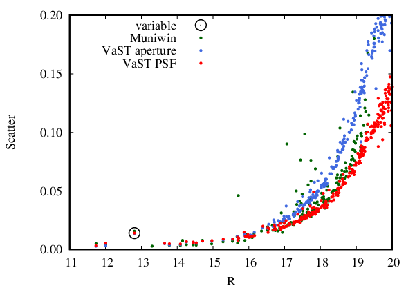
References

Acton (1996) Acton, C.H., 1996. Ancillary data services of NASA’s Navigation and Ancillary Information Facility. Planet. Space Sci. 44, 65–70.
Alard (2000) Alard, C., 2000. Image subtraction using a space-varying kernel. A&AS 144, 363–370.
Alard and Lupton (1998) Alard, C., Lupton, R.H., 1998. A Method for Optimal Image Subtraction. ApJ 503, 325–331. astro-ph/9712287.
Antipin et al. (2005) Antipin, S.V., Sokolovsky, K.V., Lebedev, A.A., 2005. GSC 02050-00745: A New RR Lyrae Star with Blazhko Effect. Information Bulletin on Variable Stars 5654.
Bacher et al. (2005) Bacher, A., Kimeswenger, S., Teutsch, P., 2005. Photometry from online Digitized Sky Survey plates. MNRAS 362, 542–548. astro-ph/0507536.
Becker (2015) Becker, A., 2015. HOTPANTS: High Order Transform of PSF ANd Template Subtraction. Astrophysics Source Code Library. 1504.004.
Belardi et al. (2016) Belardi, C., Kilic, M., Munn, J.A., Gianninas, A., Barber, S.D., Dey, A., Stetson, P.B., 2016. The DECam minute cadence survey - I. MNRAS 462, 2506–2517. 1607.08773.
Bertin (2006) Bertin, E., 2006. Automatic Astrometric and Photometric Calibration with SCAMP, in: Gabriel, C., Arviset, C., Ponz, D., Enrique, S. (Eds.), Astronomical Data Analysis Software and Systems XV, p. 112.
Bertin (2011) Bertin, E., 2011. Automated Morphometry with SExtractor and PSFEx, in: Evans, I.N., Accomazzi, A., Mink, D.J., Rots, A.H. (Eds.), Astronomical Data Analysis Software and Systems XX, p. 435.
Bertin and Arnouts (1996) Bertin, E., Arnouts, S., 1996. SExtractor: Software for source extraction. A&AS 117, 393–404.
Bertin et al. (2002) Bertin, E., Mellier, Y., Radovich, M., Missonnier, G., Didelon, P., Morin, B., 2002. The TERAPIX Pipeline, in: Bohlender, D.A., Durand, D., Handley, T.H. (Eds.), Astronomical Data Analysis Software and Systems XI, p. 228.
Bessell (2005) Bessell, M.S., 2005. Standard Photometric Systems. ARA&A 43, 293–336.
Bonanos and Boumis (2016) Bonanos, A.Z., Boumis, P., 2016. Evidence for rapid variability in the optical light curve of the Type Ia SN 2014J. A&A 585, A19. 1507.01011.
Bonnarel et al. (2000) Bonnarel, F., Fernique, P., Bienaymé, O., Egret, D., Genova, F., Louys, M., Ochsenbein, F., Wenger, M., Bartlett, J.G., 2000. The ALADIN interactive sky atlas. A reference tool for identification of astronomical sources. A&AS 143, 33–40.
Bramich et al. (2016) Bramich, D.M., Horne, K., Alsubai, K.A., Bachelet, E., Mislis, D., Parley, N., 2016. Difference image analysis: automatic kernel design using information criteria. MNRAS 457, 542–574. 1512.04655.
Breeveld et al. (2010) Breeveld, A.A., Curran, P.A., Hoversten, E.A., Koch, S., Landsman, W., Marshall, F.E., Page, M.J., Poole, T.S., Roming, P., Smith, P.J., Still, M., Yershov, V., Blustin, A.J., Brown, P.J., Gronwall, C., Holland, S.T., Kuin, N.P.M., McGowan, K., Rosen, S., Boyd, P., Broos, P., Carter, M., Chester, M.M., Hancock, B., Huckle, H., Immler, S., Ivanushkina, M., Kennedy, T., Mason, K.O., Morgan, A.N., Oates, S., de Pasquale, M., Schady, P., Siegel, M., vanden Berk, D., 2010. Further calibration of the Swift ultraviolet/optical telescope. MNRAS 406, 1687–1700. 1004.2448.
Brown et al. (2014) Brown, P.J., Breeveld, A.A., Holland, S., Kuin, P., Pritchard, T., 2014. SOUSA: the Swift Optical/Ultraviolet Supernova Archive. Ap&SS 354, 89–96. 1407.3808.
Burdanov et al. (2016) Burdanov, A.Y., Benni, P., Krushinsky, V.V., Popov, A.A., Sokov, E.N., Sokova, I.A., Rusov, S.A., Lyashenko, A.Y., Ivanov, K.I., Moiseev, A.V., Rastegaev, D.A., Dyachenko, V.V., Balega, Y.Y., Baştürk, Ö., Özavcı, I., Puchalski, D., Marchini, A., Naves, R., Shadick, S., Bretton, M., 2016. First results of the Kourovka Planet Search: discovery of transiting exoplanet candidates in the first three target fields. MNRAS 461, 3854–3863. 1607.01894.
Burdanov et al. (2014) Burdanov, A.Y., Krushinsky, V.V., Popov, A.A., 2014. Astrokit-an efficient program for high-precision differential CCD photometry and search for variable stars. Astrophysical Bulletin 69, 368–376. 1408.0664.
Chambers et al. (2016) Chambers, K.C., Magnier, E.A., Metcalfe, N., Flewelling, H.A., Huber, M.E., Waters, C.Z., Denneau, L., Draper, P.W., Farrow, D., Finkbeiner, D.P., Holmberg, C., Koppenhoefer, J., Price, P.A., Saglia, R.P., Schlafly, E.F., Smartt, S.J., Sweeney, W., Wainscoat, R.J., Burgett, W.S., Grav, T., Heasley, J.N., Hodapp, K.W., Jedicke, R., Kaiser, N., Kudritzki, R.P., Luppino, G.A., Lupton, R.H., Monet, D.G., Morgan, J.S., Onaka, P.M., Stubbs, C.W., Tonry, J.L., Banados, E., Bell, E.F., Bender, R., Bernard, E.J., Botticella, M.T., Casertano, S., Chastel, S., Chen, W.P., Chen, X., Cole, S., Deacon, N., Frenk, C., Fitzsimmons, A., Gezari, S., Goessl, C., Goggia, T., Goldman, B., Grebel, E.K., Hambly, N.C., Hasinger, G., Heavens, A.F., Heckman, T.M., Henderson, R., Henning, T., Holman, M., Hopp, U., Ip, W.H., Isani, S., Keyes, C.D., Koekemoer, A., Kotak, R., Long, K.S., Lucey, J.R., Liu, M., Martin, N.F., McLean, B., Morganson, E., Murphy, D.N.A., Nieto-Santisteban, M.A., Norberg, P., Peacock, J.A., Pier, E.A., Postman, M., Primak, N., Rae, C., Rest, A., Riess, A., Riffeser, A., Rix, H.W., Roser, S., Schilbach, E., Schultz, A.S.B., Scolnic, D., Szalay, A., Seitz, S., Shiao, B., Small, E., Smith, K.W., Soderblom, D., Taylor, A.N., Thakar, A.R., Thiel, J., Thilker, D., Urata, Y., Valenti, J., Walter, F., Watters, S.P., Werner, S., White, R., Wood-Vasey, W.M., Wyse, R., 2016. The Pan-STARRS1 Surveys. ArXiv e-prints 1612.05560.
Clementini et al. (2016) Clementini, G., Ripepi, V., Leccia, S., Mowlavi, N., Lecoeur-Taibi, I., Marconi, M., Szabados, L., Eyer, L., Guy, L.P., Rimoldini, L., Jevardat de Fombelle, G., Holl, B., Busso, G., Charnas, J., Cuypers, J., De Angeli, F., De Ridder, J., Debosscher, J., Evans, D.W., Klagyivik, P., Musella, I., Nienartowicz, K., Ordóñez, D., Regibo, S., Riello, M., Sarro, L.M., Süveges, M., 2016. Gaia Data Release 1. The Cepheid and RR Lyrae star pipeline and its application to the south ecliptic pole region. A&A 595, A133. 1609.04269.
Collins et al. (2017) Collins, K.A., Kielkopf, J.F., Stassun, K.G., Hessman, F.V., 2017. AstroImageJ: Image Processing and Photometric Extraction for Ultra-precise Astronomical Light Curves. AJ 153, 77. 1601.02622.
Cropper et al. (1989) Cropper, M., Mason, K.O., Allington-Smith, J.R., Branduardi-Raymont, G., Charles, P.A., Mittaz, J.P.D., Mukai, K., Murdin, P.G., Smale, A.P., 1989. The magnetic field in four AM HER systems - Measurements from cyclotron humps. MNRAS 236, 29P–38P.
de Diego (2010) de Diego, J.A., 2010. Testing Tests on Active Galactic Nucleus Microvariability. AJ 139, 1269–1282.
Deeg and Doyle (2001) Deeg, H.J., Doyle, L.R., 2001. VAPHOT - A Package for Precision Differential Aperture Photometry, in: Borucki, W.J., Lasher, L.E. (Eds.), Third Workshop on Photometry, p. 85.
Dékány et al. (2015) Dékány, I., Minniti, D., Majaess, D., Zoccali, M., Hajdu, G., Alonso-García, J., Catelan, M., Gieren, W., Borissova, J., 2015. The VVV Survey Reveals Classical Cepheids Tracing a Young and Thin Stellar Disk across the Galaxy’s Bulge. ApJ 812, L29. 1509.08402.
Devor et al. (2008) Devor, J., Charbonneau, D., O’Donovan, F.T., Mandushev, G., Torres, G., 2008. Identification, Classifications, and Absolute Properties of 773 Eclipsing Binaries Found in the Trans-Atlantic Exoplanet Survey. AJ 135, 850–877. 0712.0839.
Drake et al. (2009) Drake, A.J., Djorgovski, S.G., Mahabal, A., Beshore, E., Larson, S., Graham, M.J., Williams, R., Christensen, E., Catelan, M., Boattini, A., Gibbs, A., Hill, R., Kowalski, R., 2009. First Results from the Catalina Real-Time Transient Survey. ApJ 696, 870–884. 0809.1394.
Eastman et al. (2010) Eastman, J., Siverd, R., Gaudi, B.S., 2010. Achieving Better Than 1 Minute Accuracy in the Heliocentric and Barycentric Julian Dates. PASP 122, 935. 1005.4415.
Ferreira Lopes and Cross (2016) Ferreira Lopes, C.E., Cross, N.J.G., 2016. New insights into time series analysis. I. Correlated observations. A&A 586, A36. 1506.04914.
Ferreira Lopes and Cross (2017) Ferreira Lopes, C.E., Cross, N.J.G., 2017. New insights into time series analysis. II - Non-correlated observations. A&A 604, A121. 1611.07838.
Ferreira Lopes et al. (2015) Ferreira Lopes, C.E., Dékány, I., Catelan, M., Cross, N.J.G., Angeloni, R., Leão, I.C., De Medeiros, J.R., 2015. The WFCAM multiwavelength Variable Star Catalog. A&A 573, A100. 1408.4137.
Figuera Jaimes et al. (2013) Figuera Jaimes, R., Arellano Ferro, A., Bramich, D.M., Giridhar, S., Kuppuswamy, K., 2013. Variable stars in the globular cluster NGC 7492. New discoveries and physical parameter determination. A&A 556, A20. 1305.4837.
Friedrich et al. (1997) Friedrich, S., Koenig, M., Wicenec, A., 1997. Search for Variables in the TYCHO Epoch Photometry Annex B, in: Bonnet, R.M., Høg, E., Bernacca, P.L., Emiliani, L., Blaauw, A., Turon, C., Kovalevsky, J., Lindegren, L., Hassan, H., Bouffard, M., Strim, B., Heger, D., Perryman, M.A.C., Woltjer, L. (Eds.), Hipparcos - Venice ’97, pp. 441–444.
Fruth et al. (2012) Fruth, T., Kabath, P., Cabrera, J., Chini, R., Csizmadia, S., Eigmüller, P., Erikson, A., Kirste, S., Lemke, R., Murphy, M., Pasternacki, T., Rauer, H., Titz-Weider, R., 2012. Improved Variable Star Search in Large Photometric Data Sets: New Variables in CoRoT Field LRa02 Detected by BEST II. AJ 143, 140. 1205.1963.
Gaia Collaboration et al. (2016) Gaia Collaboration, Prusti, T., de Bruijne, J.H.J., Brown, A.G.A., Vallenari, A., Babusiaux, C., Bailer-Jones, C.A.L., Bastian, U., Biermann, M., Evans, D.W., et al., 2016. The Gaia mission. A&A 595, A1. 1609.04153.
Goudis et al. (2010) Goudis, C., Hantzios, P., Boumis, P., Xilouris, E., Katsiyannis, A., Maroussis, A., 2010. The Aristarchos Telescope, in: Tsinganos, K., Hatzidimitriou, D., Matsakos, T. (Eds.), 9th International Conference of the Hellenic Astronomical Society, p. 422.
Gran et al. (2016) Gran, F., Minniti, D., Saito, R.K., Zoccali, M., Gonzalez, O.A., Navarrete, C., Catelan, M., Contreras Ramos, R., Elorrieta, F., Eyheramendy, S., Jordán, A., 2016. Mapping the outer bulge with RRab stars from the VVV Survey. A&A 591, A145. 1604.01336.
Greisen and Calabretta (2002) Greisen, E.W., Calabretta, M.R., 2002. Representations of world coordinates in FITS. A&A 395, 1061–1075. astro-ph/0207407.
Grindlay et al. (2012) Grindlay, J., Tang, S., Los, E., Servillat, M., 2012. Opening the 100-Year Window for Time-Domain Astronomy, in: Griffin, E., Hanisch, R., Seaman, R. (Eds.), New Horizons in Time Domain Astronomy, pp. 29–34. 1211.1051.
Groote et al. (2014) Groote, D., Tuvikene, T., Edelmann, H., Arlt, R., Heber, U., Enke, H., 2014. Building up APPLAUSE: Digitization and web presentation of Hamburger Sternwarte plate archives, in: Astroplate 2014, p. 53.
Groth (1986) Groth, E.J., 1986. A pattern-matching algorithm for two-dimensional coordinate lists. AJ 91, 1244–1248.
Gupta et al. (2012) Gupta, A.C., Krichbaum, T.P., Wiita, P.J., Rani, B., Sokolovsky, K.V., Mohan, P., Mangalam, A., Marchili, N., Fuhrmann, L., Agudo, I., Bach, U., Bachev, R., Böttcher, M., Gabanyi, K.E., Gaur, H., Hawkins, K., Kimeridze, G.N., Kurtanidze, O.M., Kurtanidze, S.O., Lee, C.U., Liu, X., McBreen, B., Nesci, R., Nestoras, G., Nikolashvili, M.G., Ohlert, J.M., Palma, N., Peneva, S., Pursimo, T., Semkov, E., Strigachev, A., Webb, J.R., Wiesemeyer, H., Zensus, J.A., 2012. Multiwavelength intraday variability of the BL Lacertae S5 0716+714. MNRAS 425, 1357–1370. 1207.5942.
Hartman and Bakos (2016) Hartman, J.D., Bakos, G.Á., 2016. VARTOOLS: A program for analyzing astronomical time-series data. Astronomy and Computing 17, 1–72. 1605.06811.
Henden and Munari (2014) Henden, A., Munari, U., 2014. The APASS all-sky, multi-epoch BVgri photometric survey. Contributions of the Astronomical Observatory Skalnate Pleso 43, 518–522.
Henden et al. (2016) Henden, A.A., Templeton, M., Terrell, D., Smith, T.C., Levine, S., Welch, D., 2016. VizieR Online Data Catalog: AAVSO Photometric All Sky Survey (APASS) DR9 (Henden+, 2016). VizieR Online Data Catalog 2336.
Heyl (2013) Heyl, J.S., 2013. A fast matching algorithm for sheared stellar samples: k-d match. MNRAS 433, 935–939.
Hoffmann and Macri (2015) Hoffmann, S.L., Macri, L.M., 2015. Cepheid Variables in the Maser-host Galaxy NGC 4258. AJ 149, 183. 1503.07953.
Høg et al. (2000) Høg, E., Fabricius, C., Makarov, V.V., Urban, S., Corbin, T., Wycoff, G., Bastian, U., Schwekendiek, P., Wicenec, A., 2000. The Tycho-2 catalogue of the 2.5 million brightest stars. A&A 355, L27–L30.
Hogg et al. (2008) Hogg, D.W., Blanton, M., Lang, D., Mierle, K., Roweis, S., 2008. Automated Astrometry (Invited), in: Argyle, R.W., Bunclark, P.S., Lewis, J.R. (Eds.), Astronomical Data Analysis Software and Systems XVII, p. 27.
Holdsworth et al. (2014) Holdsworth, D.L., Smalley, B., Gillon, M., Clubb, K.I., Southworth, J., Maxted, P.F.L., Anderson, D.R., Barros, S.C.C., Cameron, A.C., Delrez, L., Faedi, F., Haswell, C.A., Hellier, C., Horne, K., Jehin, E., Norton, A.J., Pollacco, D., Skillen, I., Smith, A.M.S., West, R.G., Wheatley, P.J., 2014. High-frequency A-type pulsators discovered using SuperWASP. MNRAS 439, 2078–2095. 1401.3199.
Howell (2008) Howell, S.B., 2008. A tale of four surveys:What have we learned about the variable sky? Astronomische Nachrichten 329, 259.
Irwin et al. (2007) Irwin, J., Irwin, M., Aigrain, S., Hodgkin, S., Hebb, L., Moraux, E., 2007. The Monitor project: data processing and light curve production. MNRAS 375, 1449–1462. astro-ph/0612395.
Israel et al. (2015) Israel, H., Massey, R., Prod’homme, T., Cropper, M., Cordes, O., Gow, J., Kohley, R., Marggraf, O., Niemi, S., Rhodes, J., Short, A., Verhoeve, P., 2015. How well can charge transfer inefficiency be corrected? A parameter sensitivity study for iterative correction. MNRAS 453, 561–580. 1506.07831.
Jacob et al. (2010) Jacob, J.C., Katz, D.S., Berriman, G.B., Good, J., Laity, A.C., Deelman, E., Kesselman, C., Singh, G., Su, M.H., Prince, T.A., Williams, R., 2010. Montage: a grid portal and software toolkit for science-grade astronomical image mosaicking. ArXiv e-prints 1005.4454.
Jacyszyn-Dobrzeniecka et al. (2017) Jacyszyn-Dobrzeniecka, A.M., Skowron, D.M., Mróz, P., Soszyński, I., Udalski, A., Pietrukowicz, P., Skowron, J., Poleski, R., Kozłowski, S., Wyrzykowski, Ł., Pawlak, M., Szymański, M.K., Ulaczyk, K., 2017. OGLE-ing the Magellanic System: Three-Dimensional Structure of the Clouds and the Bridge using RR Lyrae Stars. Acta Astron. 67, 1–35. 1611.02709.
Jester et al. (2005) Jester, S., Schneider, D.P., Richards, G.T., Green, R.F., Schmidt, M., Hall, P.B., Strauss, M.A., Vanden Berk, D.E., Stoughton, C., Gunn, J.E., Brinkmann, J., Kent, S.M., Smith, J.A., Tucker, D.L., Yanny, B., 2005. The Sloan Digital Sky Survey View of the Palomar-Green Bright Quasar Survey. AJ 130, 873–895. astro-ph/0506022.
Kaplan et al. (1989) Kaplan, G.H., Hughes, J.A., Seidelmann, P.K., Smith, C.A., Yallop, B.D., 1989. Mean and apparent place computations in the new IAU system. III - Apparent, topocentric, and astrometric places of planets and stars. AJ 97, 1197–1210.
Karpov et al. (2012) Karpov, S., Beskin, G., Bondar, S., Perkov, A., Greco, G., Guarnieri, A., Bartolini, C., 2012. Wide and fast. Status update on FAVOR project and MegaTORTORA system, in: Astronomical Society of India Conference Series, p. 219.
Kessler et al. (2015) Kessler, R., Marriner, J., Childress, M., Covarrubias, R., D’Andrea, C.B., Finley, D.A., Fischer, J., Foley, R.J., Goldstein, D., Gupta, R.R., Kuehn, K., Marcha, M., Nichol, R.C., Papadopoulos, A., Sako, M., Scolnic, D., Smith, M., Sullivan, M., Wester, W., Yuan, F., Abbott, T., Abdalla, F.B., Allam, S., Benoit-Lévy, A., Bernstein, G.M., Bertin, E., Brooks, D., Carnero Rosell, A., Carrasco Kind, M., Castander, F.J., Crocce, M., da Costa, L.N., Desai, S., Diehl, H.T., Eifler, T.F., Fausti Neto, A., Flaugher, B., Frieman, J., Gerdes, D.W., Gruen, D., Gruendl, R.A., Honscheid, K., James, D.J., Kuropatkin, N., Li, T.S., Maia, M.A.G., Marshall, J.L., Martini, P., Miller, C.J., Miquel, R., Nord, B., Ogando, R., Plazas, A.A., Reil, K., Romer, A.K., Roodman, A., Sanchez, E., Sevilla-Noarbe, I., Smith, R.C., Soares-Santos, M., Sobreira, F., Tarle, G., Thaler, J., Thomas, R.C., Tucker, D., Walker, A.R., DES Collaboration, 2015. The Difference Imaging Pipeline for the Transient Search in the Dark Energy Survey. AJ 150, 172. 1507.05137.
Khruslov (2013) Khruslov, A.V., 2013. New Variable Stars II. Peremennye Zvezdy Prilozhenie 13, 16.
Kim et al. (2011) Kim, D.W., Protopapas, P., Alcock, C., Byun, Y.I., Khardon, R., 2011. Automatic QSO Selection Using Machine Learning: Application on Massive Astronomical Database, in: Evans, I.N., Accomazzi, A., Mink, D.J., Rots, A.H. (Eds.), Astronomical Data Analysis Software and Systems XX, p. 447.
Kolesnikova et al. (2010) Kolesnikova, D.M., Sat, L.A., Sokolovsky, K.V., Antipin, S.V., Belinskii, A.A., Samus’, N.N., 2010. New variable stars on digitized Moscow collection plates. The field of 66 Ophiuchi. Astronomy Reports 54, 1000–1018.
Kolesnikova et al. (2008) Kolesnikova, D.M., Sat, L.A., Sokolovsky, K.V., Antipin, S.V., Samus, N.N., 2008. New Variable Stars on Digitized Moscow Collection Plates. Field 66 Ophiuchi (Northern Half). Acta Astron. 58, 279–292. 0809.4153.
Korotkiy et al. (2012) Korotkiy, S., Sokolovsky, K., Brown, N.J., Gao, R.J., Seach, J., Kiytota, S., Guido, E., Howes, N., Sostero, G., Elenin, L., Molotov, I., Koff, R.A.A., Nissinen, M., Nishiyama, K., Kabashima, F., Koberger, H., Vollmann, W., Gerke, V., 2012. Nova Sagittarii 2012 = PNV J17452791-2305213. Central Bureau Electronic Telegrams 3089, 1.
Korpela (2012) Korpela, E.J., 2012. SETI@home, BOINC, and Volunteer Distributed Computing. Annual Review of Earth and Planetary Sciences 40, 69–87.
Kryachko et al. (2015) Kryachko, T., Samokhvalov, A., Satovskiy, B., 2015. Variability of TCP J04283707+3157578. Peremennye Zvezdy Prilozhenie 15, 3.
Labadie-Bartz et al. (2016) Labadie-Bartz, J., Pepper, J., McSwain, M.V., Bjorkman, J.E., Bjorkman, K.S., Lund, M.B., Rodriguez, J.E., Stassun, K.G., Stevens, D.J., Gaudi, B.S., James, D.J., Kuhn, R.B., Siverd, R.J., Beatty, T.G., 2016. Photometric Variability of the Be Star Population. ArXiv e-prints 1609.08449.
Lah et al. (2005) Lah, P., Kiss, L.L., Bedding, T.R., 2005. Red variables in the OGLE-II data base - III. Constraints on the three-dimensional structures of the Large and Small Magellanic Clouds. MNRAS 359, L42–L46. astro-ph/0502440.
Laher et al. (2014) Laher, R.R., Surace, J., Grillmair, C.J., Ofek, E.O., Levitan, D., Sesar, B., van Eyken, J.C., Law, N.M., Helou, G., Hamam, N., Masci, F.J., Mattingly, S., Jackson, E., Hacopeans, E., Mi, W., Groom, S., Teplitz, H., Desai, V., Hale, D., Smith, R., Walters, R., Quimby, R., Kasliwal, M., Horesh, A., Bellm, E., Barlow, T., Waszczak, A., Prince, T.A., Kulkarni, S.R., 2014. IPAC Image Processing and Data Archiving for the Palomar Transient Factory. PASP 126, 674. 1404.1953.
Lang et al. (2010) Lang, D., Hogg, D.W., Mierle, K., Blanton, M., Roweis, S., 2010. Astrometry.net: Blind Astrometric Calibration of Arbitrary Astronomical Images. AJ 139, 1782–1800. 0910.2233.
Lapukhin et al. (2014) Lapukhin, E.G., Veselkov, S.A., Zubareva, A.M., Starovoit, E.D., Kolbasina, I.V., 2014. New Variable Stars in Lacerta: Area of $2^{\circ}.3\times 2^{\circ}$ .3, Centered at $\alpha=$ 22h50m, $\delta=50^{\circ}00\prime$ (2000.0). Part III. Peremennye Zvezdy Prilozhenie 14, 12.
Majaess et al. (2013) Majaess, D., Carraro, G., Moni Bidin, C., Bonatto, C., Berdnikov, L., Balam, D., Moyano, M., Gallo, L., Turner, D., Lane, D., Gieren, W., Borissova, J., Kovtyukh, V., Beletsky, Y., 2013. Anchors for the cosmic distance scale: the Cepheids U Sagittarii, CF Cassiopeiae, and CEab Cassiopeiae. A&A 560, A22. 1311.0865.
Mason et al. (2001) Mason, K.O., Breeveld, A., Much, R., Carter, M., Cordova, F.A., Cropper, M.S., Fordham, J., Huckle, H., Ho, C., Kawakami, H., Kennea, J., Kennedy, T., Mittaz, J., Pandel, D., Priedhorsky, W.C., Sasseen, T., Shirey, R., Smith, P., Vreux, J.M., 2001. The XMM-Newton optical/UV monitor telescope. A&A 365, L36–L44. astro-ph/0011216.
Mauro et al. (2015) Mauro, F., Bidin, C.M., Chené, A., Geisler, D., Alonso-García, J., Borissova, J., Carraro, G., 2015. The VVV-SkZ Pipeline: How to Get Automatic PSF-Fitting Photometry from the VVV Survey, in: Points, S., Kunder, A. (Eds.), Fifty Years of Wide Field Studies in the Southern Hemisphere: Resolved Stellar Populations of the Galactic Bulge and Magellanic Clouds, p. 83.
McQuillin et al. (2012) McQuillin, R., Evans, A., Wilson, D., Maxted, P.F.L., Pollacco, D., West, R.G., Hounsell, R.A., Bode, M.F., 2012. Novae in the SuperWASP data base. MNRAS 419, 330–335.
Mighell (1999) Mighell, K.J., 1999. Algorithms for CCD Stellar Photometry, in: Mehringer, D.M., Plante, R.L., Roberts, D.A. (Eds.), Astronomical Data Analysis Software and Systems VIII, p. 317.
Mink (1997) Mink, D.J., 1997. WCSTools: Image World Coordinate System Utilities, in: Hunt, G., Payne, H. (Eds.), Astronomical Data Analysis Software and Systems VI, p. 249.
Mink (2014) Mink, J., 2014. WCSTools: Catalogs, Headers, and FITS Files, Oh My!, in: Manset, N., Forshay, P. (Eds.), Astronomical Data Analysis Software and Systems XXIII, p. 231.
Minniti et al. (2010) Minniti, D., Lucas, P.W., Emerson, J.P., Saito, R.K., Hempel, M., Pietrukowicz, P., Ahumada, A.V., Alonso, M.V., Alonso-Garcia, J., Arias, J.I., Bandyopadhyay, R.M., Barbá, R.H., Barbuy, B., Bedin, L.R., Bica, E., Borissova, J., Bronfman, L., Carraro, G., Catelan, M., Clariá, J.J., Cross, N., de Grijs, R., Dékány, I., Drew, J.E., Fariña, C., Feinstein, C., Fernández Lajús, E., Gamen, R.C., Geisler, D., Gieren, W., Goldman, B., Gonzalez, O.A., Gunthardt, G., Gurovich, S., Hambly, N.C., Irwin, M.J., Ivanov, V.D., Jordán, A., Kerins, E., Kinemuchi, K., Kurtev, R., López-Corredoira, M., Maccarone, T., Masetti, N., Merlo, D., Messineo, M., Mirabel, I.F., Monaco, L., Morelli, L., Padilla, N., Palma, T., Parisi, M.C., Pignata, G., Rejkuba, M., Roman-Lopes, A., Sale, S.E., Schreiber, M.R., Schröder, A.C., Smith, M., , Jr., L.S., Soto, M., Tamura, M., Tappert, C., Thompson, M.A., Toledo, I., Zoccali, M., Pietrzynski, G., 2010. VISTA Variables in the Via Lactea (VVV): The public ESO near-IR variability survey of the Milky Way. New A 15, 433–443. 0912.1056.
Mommert (2017) Mommert, M., 2017. PHOTOMETRYPIPELINE: An automated pipeline for calibrated photometry. Astronomy and Computing 18, 47–53. 1702.00834.
Monet et al. (2003) Monet, D.G., Levine, S.E., Canzian, B., Ables, H.D., Bird, A.R., Dahn, C.C., Guetter, H.H., Harris, H.C., Henden, A.A., Leggett, S.K., Levison, H.F., Luginbuhl, C.B., Martini, J., Monet, A.K.B., Munn, J.A., Pier, J.R., Rhodes, A.R., Riepe, B., Sell, S., Stone, R.C., Vrba, F.J., Walker, R.L., Westerhout, G., Brucato, R.J., Reid, I.N., Schoening, W., Hartley, M., Read, M.A., Tritton, S.B., 2003. The USNO-B Catalog. AJ 125, 984–993. astro-ph/0210694.
Mowlavi (2014) Mowlavi, N., 2014. Searching transients in large-scale surveys. A method based on the Abbe value. A&A 568, A78. 1406.7785.
Mukai (2017) Mukai, K., 2017. X-Ray Emissions from Accreting White Dwarfs: a Review. PASP 129, 062001. 1703.06171.
Nandra et al. (1997) Nandra, K., George, I.M., Mushotzky, R.F., Turner, T.J., Yaqoob, T., 1997. ASCA Observations of Seyfert 1 Galaxies. I. Data Analysis, Imaging, and Timing. ApJ 476, 70–82.
Nethercote and Seward (2007) Nethercote, N., Seward, J., 2007. Valgrind: A framework for heavyweight dynamic binary instrumentation, in: Proceedings of ACM SIGPLAN 2007 Conference on Programming Language Design and Implementation (PLDI 2007), San Diego, California, USA. pp. 89–100.
Nethercote et al. (2006) Nethercote, N., Walsh, R., Fitzhardinge, J., 2006. Building workload characterization tools with Valgrind, in: Invited tutorial, IEEE International Symposium on Workload Characterization (IISWC 2006), San José, California, USA.
von Neumann (1941) von Neumann, J., 1941. Distribution of the ratio of the mean square successive difference to the variance. Ann. Math. Statist. 12, 367–395.
Norton et al. (2016) Norton, A.J., Lohr, M.E., Smalley, B., Wheatley, P.J., West, R.G., 2016. SuperWASP discovery and SALT confirmation of a semi-detached eclipsing binary that contains a $\delta$ Scuti star. A&A 587, A54. 1601.03198.
Norton et al. (2011) Norton, A.J., Payne, S.G., Evans, T., West, R.G., Wheatley, P.J., Anderson, D.R., Barros, S.C.C., Butters, O.W., Collier Cameron, A., Christian, D.J., Enoch, B., Faedi, F., Haswell, C.A., Hellier, C., Holmes, S., Horne, K.D., Kane, S.R., Lister, T.A., Maxted, P.F.L., Parley, N., Pollacco, D., Simpson, E.K., Skillen, I., Smalley, B., Southworth, J., Street, R.A., 2011. Short period eclipsing binary candidates identified using SuperWASP. A&A 528, A90. 1101.1223.
Ochsenbein et al. (2000) Ochsenbein, F., Bauer, P., Marcout, J., 2000. The VizieR database of astronomical catalogues. A&AS 143, 23–32. astro-ph/0002122.
Osaki (1996) Osaki, Y., 1996. Dwarf-Nova Outbursts. PASP 108, 39.
Pál (2012) Pál, A., 2012. FITSH- a software package for image processing. MNRAS 421, 1825–1837. 1111.1998.
Pál and Bakos (2006) Pál, A., Bakos, G.Á., 2006. Astrometry in Wide-Field Surveys. PASP 118, 1474–1483. astro-ph/0609658.
Parks et al. (2014) Parks, J.R., Plavchan, P., White, R.J., Gee, A.H., 2014. Periodic and Aperiodic Variability in the Molecular Cloud $\rho$ Ophiuchus. ApJS 211, 3. 1309.5300.
Pashchenko et al. (2017) Pashchenko, I.N., Sokolovsky, K.V., Gavras, P., 2017. Machine learning search for variable stars. ArXiv:1710.07290 1710.07290.
Pietrukowicz et al. (2015) Pietrukowicz, P., Kozłowski, S., Skowron, J., Soszyński, I., Udalski, A., Poleski, R., Wyrzykowski, Ł., Szymański, M.K., Pietrzyński, G., Ulaczyk, K., Mróz, P., Skowron, D.M., Kubiak, M., 2015. Deciphering the 3D Structure of the Old Galactic Bulge from the OGLE RR Lyrae Stars. ApJ 811, 113. 1412.4121.
Pojmanski (1997) Pojmanski, G., 1997. The All Sky Automated Survey. Acta Astron. 47, 467–481. astro-ph/9712146.
Pojmanski (2002) Pojmanski, G., 2002. The All Sky Automated Survey. Catalog of Variable Stars. I. 0 h - 6 hQuarter of the Southern Hemisphere. Acta Astron. 52, 397–427. astro-ph/0210283.
Poole et al. (2008) Poole, T.S., Breeveld, A.A., Page, M.J., Landsman, W., Holland, S.T., Roming, P., Kuin, N.P.M., Brown, P.J., Gronwall, C., Hunsberger, S., Koch, S., Mason, K.O., Schady, P., vanden Berk, D., Blustin, A.J., Boyd, P., Broos, P., Carter, M., Chester, M.M., Cucchiara, A., Hancock, B., Huckle, H., Immler, S., Ivanushkina, M., Kennedy, T., Marshall, F., Morgan, A., Pandey, S.B., de Pasquale, M., Smith, P.J., Still, M., 2008. Photometric calibration of the Swift ultraviolet/optical telescope. MNRAS 383, 627–645. 0708.2259.
Reid et al. (2001) Reid, M.L., Sullivan, D.J., Dodd, R.J., 2001. A High Throughput Photometric Pipeline, in: Harnden, Jr., F.R., Primini, F.A., Payne, H.E. (Eds.), Astronomical Data Analysis Software and Systems X, p. 306.
Riccio et al. (2017) Riccio, G., Brescia, M., Cavuoti, S., Mercurio, A., di Giorgio, A.M., Molinari, S., 2017. C ³, A Command-line Catalog Cross-match Tool for Large Astrophysical Catalogs. PASP 129, 024005. 1611.04431.
Ricker et al. (2015) Ricker, G.R., Winn, J.N., Vanderspek, R., Latham, D.W., Bakos, G.Á., Bean, J.L., Berta-Thompson, Z.K., Brown, T.M., Buchhave, L., Butler, N.R., Butler, R.P., Chaplin, W.J., Charbonneau, D., Christensen-Dalsgaard, J., Clampin, M., Deming, D., Doty, J., De Lee, N., Dressing, C., Dunham, E.W., Endl, M., Fressin, F., Ge, J., Henning, T., Holman, M.J., Howard, A.W., Ida, S., Jenkins, J.M., Jernigan, G., Johnson, J.A., Kaltenegger, L., Kawai, N., Kjeldsen, H., Laughlin, G., Levine, A.M., Lin, D., Lissauer, J.J., MacQueen, P., Marcy, G., McCullough, P.R., Morton, T.D., Narita, N., Paegert, M., Palle, E., Pepe, F., Pepper, J., Quirrenbach, A., Rinehart, S.A., Sasselov, D., Sato, B., Seager, S., Sozzetti, A., Stassun, K.G., Sullivan, P., Szentgyorgyi, A., Torres, G., Udry, S., Villasenor, J., 2015. Transiting Exoplanet Survey Satellite (TESS). Journal of Astronomical Telescopes, Instruments, and Systems 1, 014003.
Ridgway et al. (2014) Ridgway, S.T., Matheson, T., Mighell, K.J., Olsen, K.A., Howell, S.B., 2014. The Variable Sky of Deep Synoptic Surveys. ApJ 796, 53. 1409.3265.
Roberts et al. (2013) Roberts, S., McQuillan, A., Reece, S., Aigrain, S., 2013. Astrophysically robust systematics removal using variational inference: application to the first month of Kepler data. MNRAS 435, 3639–3653. 1308.3644.
Rodriguez et al. (2013) Rodriguez, J.E., Pepper, J., Stassun, K.G., Siverd, R.J., Cargile, P., Beatty, T.G., Gaudi, B.S., 2013. Occultation of the T Tauri Star RW Aurigae A by its Tidally Disrupted Disk. AJ 146, 112. 1308.2017.
Rose and Hintz (2007) Rose, M.B., Hintz, E.G., 2007. A Search for Low-Amplitude Variability in Six Open Clusters Using the Robust Median Statistic. AJ 134, 2067–2078.
Rozyczka et al. (2017) Rozyczka, M., Thompson, I.B., Pych, W., Narloch, W., Poleski, R., Schwarzenberg-Czerny, A., 2017. The Cluster AgeS Experiment (CASE). Variable stars in the field of the globular cluster M22. ArXiv e-prints 1709.09572.
Russell et al. (2016) Russell, T.D., Miller-Jones, J.C.A., Sivakoff, G.R., Altamirano, D., O’Brien, T.J., Page, K.L., Templeton, M.R., Körding, E.G., Knigge, C., Rupen, M.P., Fender, R.P., Heinz, S., Maitra, D., Markoff, S., Migliari, S., Remillard, R.A., Russell, D.M., Sarazin, C.L., Waagen, E.O., 2016. The reproducible radio outbursts of SS Cygni. MNRAS 460, 3720–3732. 1605.07136.
Samus and Antipin (2015) Samus, N.N., Antipin, S.V., 2015. Variable Stars and Data-Intensive Astronomy. Highlights of Astronomy 16, 687–688.
Samus et al. (2009) Samus, N.N., Durlevich, O.V., Goranskij, V.P., Kazarovets, E.V., Kireeva, N.N., Pastukhova, E.N., Zharova, A.V., 2009. General Catalogue of Variable Stars (Samus+ 2007-2015). VizieR Online Catalog B/gcvs .
Schinzel et al. (2011) Schinzel, F.K., Sokolovsky, K.V., D’Ammando, F., Burnett, T.H., Max-Moerbeck, W., Cheung, C.C., Fegan, S.J., Casandjian, J.M., Reyes, L.C., Villata, M., Raiteri, C.M., Agudo, I., Bravo Calle, O.J.A., Carosati, D., Casas, R., Gómez, J.L., Gurwell, M.A., Hsiao, H.Y., Jorstad, S.G., Kimeridze, G., Konstantinova, T.S., Kopatskaya, E.N., Koptelova, E., Kurtanidze, O.M., Kurtanidze, S.O., Larionov, V.M., Larionova, E.G., Larionova, L.V., Marscher, A.P., Morozova, D.A., Nikolashvili, M.G., Roca-Sogorb, M., Ros, J.A., Sigua, L.A., Spiridonova, O., Troitsky, I.S., Vlasyuk, V.V., Lobanov, A.P., Zensus, J.A., 2011. Identification of $\gamma$ -ray emission from 3C 345 and NRAO 512. A&A 532, A150. 1107.2926.
Sergey et al. (2014) Sergey, I., Bryukhanov, I., Balyuk, I., 2014. 59 New Red Variable Stars. Peremennye Zvezdy Prilozhenie 14, 4.
Seward and Nethercote (2005) Seward, J., Nethercote, N., 2005. Using valgrind to detect undefined value errors with bit-precision, in: Proceedings of the USENIX’05 Annual Technical Conference, Anaheim, California, USA.
Sherwood and Plaut (1975) Sherwood, V.E., Plaut, L. (Eds.), 1975. Variable stars and stellar evolution; Proceedings of the Symposium, Moskovskii Gosudarstvennyi Universitet, Moscow, USSR, July 29-August 4, 1974. volume 67 of IAU Symposium.
Shin et al. (2009) Shin, M.S., Sekora, M., Byun, Y.I., 2009. Detecting variability in massive astronomical time series data - I. Application of an infinite Gaussian mixture model. MNRAS 400, 1897–1910. 0908.2664.
Shupe et al. (2012) Shupe, D.L., Laher, R.R., Storrie-Lombardi, L., Surace, J., Grillmair, C., Levitan, D., Sesar, B., 2012. More flexibility in representing geometric distortion in astronomical images, in: Software and Cyberinfrastructure for Astronomy II, p. 84511M.
Shupe et al. (2005) Shupe, D.L., Moshir, M., Li, J., Makovoz, D., Narron, R., Hook, R.N., 2005. The SIP Convention for Representing Distortion in FITS Image Headers, in: Shopbell, P., Britton, M., Ebert, R. (Eds.), Astronomical Data Analysis Software and Systems XIV, p. 491.
Sokolovsky et al. (2014a) Sokolovsky, K., Antipin, S., Kolesnikova, D., Lebedev, A., Samus, N., Sat, L., Zubareva, A., 2014a. A search for new variable stars using digitized Moscow collection plates, in: Astroplate 2014, p. 79. 1403.5334.
Sokolovsky et al. (2012) Sokolovsky, K., Korotkiy, S., Elenin, L., Molotov, I., 2012. Swift observation of the nova candidate PNV J17452791-2305213 one day after discovery. The Astronomer’s Telegram 4061.
Sokolovsky et al. (2014b) Sokolovsky, K., Korotkiy, S., Lebedev, A., 2014b. The New Milky Way: A Wide-Field Survey of Optical Transients near the Galactic plane, in: Woudt, P.A., Ribeiro, V.A.R.M. (Eds.), Stellar Novae: Past and Future Decades, p. 395. 1303.3268.
Sokolovsky and Lebedev (2005) Sokolovsky, K., Lebedev, A., 2005. POISK - a SExtractor front-end for search of variable objects in series of ccd images, in: Simon, A., Golovin, A. (Eds.), 12th Young Scientists’ Conference on Astronomy and Space Physics, p. 79.
Sokolovsky et al. (2010) Sokolovsky, K., Maceroni, C., Hareter, M., Damiani, C., Balaguer-Núñez, L., Ribas, I., 2010. A new eclipsing binary system with a pulsating component detected by CoRoT. Communications in Asteroseismology 161, 55–70. 1006.3050.
Sokolovsky (2009) Sokolovsky, K.V., 2009. Three New Eclipsing Binaries Near the Galactic Center. Peremennye Zvezdy Prilozhenie 9.
Sokolovsky et al. (2011) Sokolovsky, K.V., Antipin, S.V., Zharova, A., Korotkiy, S.A., 2011. GSC 2576-02071 and GSC 2576-01248: two Algol-type eclipsing binaries studied using CCD observations and historical photographic data. Peremennye Zvezdy 31. 1101.3741.
Sokolovsky et al. (2014c) Sokolovsky, K.V., Antipin, S.V., Zubareva, A.M., Kolesnikova, D.M., Lebedev, A.A., Samus’, N.N., Sat, L.A., 2014c. New variable stars on digitized plates of the Moscow collection. Field SA9. Astronomy Reports 58, 319–327.
Sokolovsky et al. (2017) Sokolovsky, K.V., Gavras, P., Karampelas, A., Antipin, S.V., Bellas-Velidis, I., Benni, P., Bonanos, A.Z., Burdanov, A.Y., Derlopa, S., Hatzidimitriou, D., Khokhryakova, A.D., Kolesnikova, D.M., Korotkiy, S.A., Lapukhin, E.G., Moretti, M.I., Popov, A.A., Pouliasis, E., Samus, N.N., Spetsieri, Z., Veselkov, S.A., Volkov, K.V., Yang, M., Zubareva, A.M., 2017. Comparative performance of selected variability detection techniques in photometric time series data. MNRAS 464, 274–292. 1609.01716.
Sokolovsky et al. (2016) Sokolovsky, K.V., Kolesnikova, D.M., Zubareva, A.M., Samus, N.N., Antipin, S.V., 2016. Variable stars identification in digitized photographic data. ArXiv e-prints 1605.03571.
Sokolovsky et al. (2009) Sokolovsky, K.V., Kovalev, Y.Y., Kovalev, Y.A., Nizhelskiy, N.A., Zhekanis, G.V., 2009. A sample of GHz-peaked spectrum sources selected at RATAN-600: Spectral and variability properties. Astronomische Nachrichten 330, 199. 0901.1064.
Sokolovsky et al. (2014d) Sokolovsky, K.V., Schinzel, F.K., Tanaka, Y.T., Abolmasov, P.K., Angelakis, E., Bulgarelli, A., Carrasco, L., Cenko, S.B., Cheung, C.C., Clubb, K.I., D’Ammando, F., Escande, L., Fegan, S.J., Filippenko, A.V., Finke, J.D., Fuhrmann, L., Fukazawa, Y., Hays, E., Healey, S.E., Ikejiri, Y., Itoh, R., Kawabata, K.S., Komatsu, T., Kovalev, Y.A., Kovalev, Y.Y., Krichbaum, T.P., Larsson, S., Lister, M.L., Lott, B., Max-Moerbeck, W., Nestoras, I., Pittori, C., Pursimo, T., Pushkarev, A.B., Readhead, A.C.S., Recillas, E., Richards, J.L., Riquelme, D., Romani, R.W., Sakimoto, K., Sasada, M., Schmidt, R., Shaw, M.S., Sievers, A., Thompson, D.J., Uemura, M., Ungerechts, H., Vercellone, S., Verrecchia, F., Yamanaka, M., Yoshida, M., Zensus, J.A., 2014d. Two active states of the narrow-line gamma-ray-loud AGN GB 1310+487. A&A 565, A26. 1401.2151.
Stetson (1996) Stetson, P.B., 1996. On the Automatic Determination of Light-Curve Parameters for Cepheid Variables. PASP 108, 851.
Subramanian and Subramaniam (2012) Subramanian, S., Subramaniam, A., 2012. The Three-dimensional Structure of the Small Magellanic Cloud. ApJ 744, 128. 1109.3980.
Swinbank et al. (2015) Swinbank, J.D., Staley, T.D., Molenaar, G.J., Rol, E., Rowlinson, A., Scheers, B., Spreeuw, H., Bell, M.E., Broderick, J.W., Carbone, D., Garsden, H., van der Horst, A.J., Law, C.J., Wise, M., Breton, R.P., Cendes, Y., Corbel, S., Eislöffel, J., Falcke, H., Fender, R., Grießmeier, J.M., Hessels, J.W.T., Stappers, B.W., Stewart, A.J., Wijers, R.A.M.J., Wijnands, R., Zarka, P., 2015. The LOFAR Transients Pipeline. Astronomy and Computing 11, 25–48. 1503.01526.
Tabur (2007) Tabur, V., 2007. Fast Algorithms for Matching CCD Images to a Stellar Catalogue. PASA 24, 189–198. 0710.3618.
Tamuz et al. (2005) Tamuz, O., Mazeh, T., Zucker, S., 2005. Correcting systematic effects in a large set of photometric light curves. MNRAS 356, 1466–1470. astro-ph/0502056.
Tang et al. (2013) Tang, S., Grindlay, J., Los, E., Servillat, M., 2013. Improved Photometry for the DASCH Pipeline. PASP 125, 857–865. 1304.7504.
Terrón and Fernández (2011) Terrón, V., Fernández, M., 2011. LEMON: an (almost) completely automated differential-photometry pipeline, in: Zapatero Osorio, M.R., Gorgas, J., Maíz Apellániz, J., Pardo, J.R., Gil de Paz, A. (Eds.), Highlights of Spanish Astrophysics VI, pp. 755–761.
Tody (1986) Tody, D., 1986. The IRAF Data Reduction and Analysis System, in: Crawford, D.L. (Ed.), Instrumentation in astronomy VI, p. 733.
Torres et al. (2010) Torres, G., Andersen, J., Giménez, A., 2010. Accurate masses and radii of normal stars: modern results and applications. A&A Rev. 18, 67–126. 0908.2624.
Tuvikene et al. (2014) Tuvikene, T., Edelmann, H., Groote, D., Enke, H., 2014. Work flow for plate digitization, data extraction and publication, in: Astroplate 2014, p. 127.
Valdes et al. (1995) Valdes, F.G., Campusano, L.E., Velasquez, J.D., Stetson, P.B., 1995. FOCAS Automatic Catalog Matching Algorithms. PASP 107, 1119.
Vicente et al. (2007) Vicente, B., Abad, C., Garzón, F., 2007. Astrometry with Carte du Ciel plates, San Fernando zone. I. Digitization and measurement using a flatbed scanner. A&A 471, 1077–1089. 0706.1900.
Watson (2006) Watson, C.L., 2006. The International Variable Star Index (VSX). Society for Astronomical Sciences Annual Symposium 25, 47.
Welch and Stetson (1993) Welch, D.L., Stetson, P.B., 1993. Robust variable star detection techniques suitable for automated searches - New results for NGC 1866. AJ 105, 1813–1821.
Wenger et al. (2000) Wenger, M., Ochsenbein, F., Egret, D., Dubois, P., Bonnarel, F., Borde, S., Genova, F., Jasniewicz, G., Laloë, S., Lesteven, S., Monier, R., 2000. The SIMBAD astronomical database. The CDS reference database for astronomical objects. A&AS 143, 9–22. astro-ph/0002110.
Wertz et al. (2016) Wertz, M., Horns, D., Groote, D., Tuvikene, T., Czesla, S., Schmitt, J.H.M.M., 2016. Hamburger Sternwarte plate archives: Historic long-term variability study of active galaxies based on digitized photographic plates. ArXiv e-prints 1607.00312.
Wheatley et al. (2017) Wheatley, P.J., West, R.G., Goad, M.R., Jenkins, J.S., Pollacco, D.L., Queloz, D., Rauer, H., Udry, S., Watson, C.A., Chazelas, B., Eigmuller, P., Lambert, G., Genolet, L., McCormac, J., Walker, S., Armstrong, D.J., Bayliss, D., Bento, J., Bouchy, F., Burleigh, M.R., Cabrera, J., Casewell, S.L., Chaushev, A., Chote, P., Csizmadia, S., Erikson, A., Faedi, F., Foxell, E., Gansicke, B.T., Gillen, E., Grange, A., Gunther, M.N., Hodgkin, S.T., Jackman, J., Jordan, A., Louden, T., Metrailler, L., Moyano, M., Nielsen, L.D., Osborn, H.P., Poppenhaeger, K., Raddi, R., Raynard, L., Smith, A.M.S., Soto, M., Titz-Weider, R., 2017. The Next Generation Transit Survey (NGTS). ArXiv:1710.11100 1710.11100.
Wilson et al. (2012) Wilson, G., Aruliah, D.A., Titus Brown, C., Chue Hong, N.P., Davis, M., Guy, R.T., Haddock, S.H.D., Huff, K., Mitchell, I.M., Plumbley, M., Waugh, B., White, E.P., Wilson, P., 2012. Best Practices for Scientific Computing. ArXiv e-prints 1210.0530.
Wozniak (2000) Wozniak, P.R., 2000. Difference Image Analysis of the OGLE-II Bulge Data. I. The Method. Acta Astron. 50, 421–450. astro-ph/0012143.
Woźniak et al. (2004) Woźniak, P.R., Vestrand, W.T., Akerlof, C.W., Balsano, R., Bloch, J., Casperson, D., Fletcher, S., Gisler, G., Kehoe, R., Kinemuchi, K., Lee, B.C., Marshall, S., McGowan, K.E., McKay, T.A., Rykoff, E.S., Smith, D.A., Szymanski, J., Wren, J., 2004. Northern Sky Variability Survey: Public Data Release. AJ 127, 2436–2449. astro-ph/0401217.
Wright et al. (2010) Wright, E.L., Eisenhardt, P.R.M., Mainzer, A.K., Ressler, M.E., Cutri, R.M., Jarrett, T., Kirkpatrick, J.D., Padgett, D., McMillan, R.S., Skrutskie, M., Stanford, S.A., Cohen, M., Walker, R.G., Mather, J.C., Leisawitz, D., Gautier, III, T.N., McLean, I., Benford, D., Lonsdale, C.J., Blain, A., Mendez, B., Irace, W.R., Duval, V., Liu, F., Royer, D., Heinrichsen, I., Howard, J., Shannon, M., Kendall, M., Walsh, A.L., Larsen, M., Cardon, J.G., Schick, S., Schwalm, M., Abid, M., Fabinsky, B., Naes, L., Tsai, C.W., 2010. The Wide-field Infrared Survey Explorer (WISE): Mission Description and Initial On-orbit Performance. AJ 140, 1868–1881. 1008.0031.
Wyrzykowski et al. (2009) Wyrzykowski, Ł., Kozłowski, S., Skowron, J., Belokurov, V., Smith, M.C., Udalski, A., Szymański, M.K., Kubiak, M., Pietrzyński, G., Soszyński, I., Szewczyk, O., Żebruń, K., 2009. The OGLE view of microlensing towards the Magellanic Clouds - I. A trickle of events in the OGLE-II LMC data. MNRAS 397, 1228–1242. 0905.2044.
Zacharias et al. (2015) Zacharias, N., Finch, C., Subasavage, J., Bredthauer, G., Crockett, C., Divittorio, M., Ferguson, E., Harris, F., Harris, H., Henden, A., Kilian, C., Munn, J., Rafferty, T., Rhodes, A., Schultheiss, M., Tilleman, T., Wieder, G., 2015. The First U.S. Naval Observatory Robotic Astrometric Telescope Catalog. AJ 150, 101. 1508.04637.
Zacharias et al. (2013) Zacharias, N., Finch, C.T., Girard, T.M., Henden, A., Bartlett, J.L., Monet, D.G., Zacharias, M.I., 2013. The Fourth US Naval Observatory CCD Astrograph Catalog (UCAC4). AJ 145, 44. 1212.6182.
Zhang et al. (2016) Zhang, M., Bakos, G.Á., Penev, K., Csubry, Z., Hartman, J.D., Bhatti, W., de Val-Borro, M., 2016. Precision Multiband Photometry with a DSLR Camera. PASP 128, 035001. 1506.03097.
Zinn et al. (2017) Zinn, J.C., Kochanek, C.S., Kozłowski, S., Udalski, A., Szymański, M.K., Soszyński, I., Wyrzykowski, Ł., Ulaczyk, K., Poleski, R., Pietrukowicz, P., Skowron, J., Mróz, P., Pawlak, M., 2017. Variable classification in the LSST era: exploring a model for quasi-periodic light curves. MNRAS 468, 2189–2205. 1612.04834.

VaST: a variability search toolkit⋆

Abstract

Keywords:

1 Introduction

2 VaST design and the challenge of variability detection

3 Data processing flow

3.1 Reading metadata from the FITS header

3.2 Source extraction and photometry

3.3 Cross-matching source lists

3.4 Cross-calibration of instrumental magnitudes

3.5 Output lightcurves, statistics and the graphical interface

3.6 Processing time

3.7 Astrometric calibration

3.8 Photometric calibration

3.9 Flag images

4 Searching for transients with VaST

5 Remarks on development process

6 VaST applications

7 Summary

Acknowledgments

Appendix A Use cases

A.1 Compiling VaST

A.2 Variability search in a series of CCD images

A.3 Setting a reference image of your choice

A.4 Restarting work after a break

A.5 View a lightcurve of an individual star

A.6 Manual single-star magnitude calibration

A.7 Automated magnitude scale calibration

A.8 Fine-tuning source extraction parameters

A.9 Selecting best aperture size for each source

A.10 PSF-fitting photometry with PSFEx

A.11 Improving photometric accuracy with SysRem

A.12 Variability search with photographic plates

A.13 Identification of a variable object

A.14 Importing lightcurves from other software

A.15 Transient detection

A.16 Heliocentric correction

A.17 Re-formatting a lightcurve for publication

A.18 Split multi-extension FITS image

Appendix B Command line options

Appendix C Log files

Appendix D Comparison with AstroImageJ and Muniwin

References

VaST: a variability search toolkit^⋆