Finite-time generalization of the thermodynamic uncertainty relation

Patrick Pietzonka Affiliation: II. Institut für Theoretische Physik, Universität Stuttgart, 70550 Stuttgart, Germany Felix Ritort Affiliation: Departament de Física Fonamental, Universitat de Barcelona, Diagonal 647, 08028 Barcelona, Spain Affiliation: CIBER-BBN de Bioingeniería, Biomateriales y Nanomedicina, Instituto de Salud Carlos III, 28029 Madrid, Spain Udo Seifert Affiliation: II. Institut für Theoretische Physik, Universität Stuttgart, 70550 Stuttgart, Germany

August 24, 2026

Abstract

For fluctuating currents in non-equilibrium steady states, the recently discovered thermodynamic uncertainty relation expresses a fundamental relation between their variance and the overall entropic cost associated with the driving. We show that this relation holds not only for the long-time limit of fluctuations, as described by large deviation theory, but also for fluctuations on arbitrary finite time scales. This generalization facilitates applying the thermodynamic uncertainty relation to single molecule experiments, for which infinite timescales are not accessible. Importantly, often this finite-time variant of the relation allows inferring a bound on the entropy production that is even stronger than the one obtained from the long-time limit. We illustrate the relation for the fluctuating work that is performed by a stochastically switching laser tweezer on a trapped colloidal particle.

pacs

05.70.Ln, 05.40.-a

I Introduction

The arguably most prominent characteristics of a thermal system driven into a non-equilibrium steady state (NESS) is its rate of entropy production $\sigma$ , i.e., the amount of heat that is transferred to a heat bath per unit of time. For an exact experimental determination of $\sigma$ , however, one would have to measure either the temperature change of a large but yet finite heat bath or to keep track of the net (free) energy input of all the driving forces. For micro- and nano-systems, such as present in single molecule or soft matter experiments [1, 2, 3], the temperature changes of a macroscopic heat bath are by far too small for the first method to be feasible. The second method is viable only if the system is driven by mechanical forces acting on observable degrees of freedom or for small electronic circuits [4, 5]. However, the quantitative energetic input of chemical driving maintained by macroscopic particle reservoirs, so-called chemostats, is not yet accessible on a molecular scale.

A lower bound on $\sigma$ can be inferred from the recently discovered thermodynamic uncertainty relation by measuring the mean and variance of an arbitrary non-vanishing current in a NESS [6, 7]. Turning the argument around, in situations where $\sigma$ is directly accessible, the thermodynamic uncertainty can be used to predict the minimal variance of any current. So far, this relation has been understood in the context of large deviation theory [8, 9, 10, 7, 11], which has led to refinements [12, 13] and variants for the diffusion in periodic potentials [14], stochastic pumps [15], and first passage problems [16]. Moreover, the thermodynamic uncertainty relation has been considered theoretically in such diverse contexts as enzyme kinetics [17], self-propelled particles [18], magnetic systems [19], self-assembly [20], Brownian clocks [21], and the efficiency of molecular motors [22].

The thermodynamic uncertainty relation as established so far, crucially relying on large deviation theory, considers fluctuations that occur in the limiting case of large time scales. Estimating large deviation functions experimentally is possible on the basis of large sets of data and if the probability of untypical fluctuations decays slowly enough to make the long time limit accessible [23]. In contrast, the theory of stochastic thermodynamics [3] has proven most fruitful for experimental applications in cases where it provides relations that hold on finite time scales. Most prominently, the Jarzynski relation [24] and the Crooks fluctuation theorem [25] allow one to infer free energy differences from the measurement of the fluctuating work during finite-time protocols, see, e.g., [26]. Similarly, the concept of stochastic entropy [27] allows for a generalization of the detailed fluctuation theorem for the entropy production in a NESS [28] to finite and thus experimentally accessible time scales [29].

In this paper, we show, based on extensive numerical evidence, that the thermodynamic uncertainty relation can be generalized to fluctuations on finite time scales as well. We illustrate this finite-time version with experimental data for fluctuations of work performed on a colloidal particle in a dichotomously switching trap [30, 31, 32]. This illustration serves as a proof of principle for applying the uncertainty relation in the future to more complex experimental systems with more than one input or output current such as Brownian heat engines [33, 23] and molecular motors, see, e.g., [34]. For small electronic circuits at low temperature this approach may become complementary to the recent progress in calorimetrically measuring heat transfer [4, 5].

The paper is organized as follows. In Sec. II we state the main result, which is then illustrated experimentally in Sec. III. In Sec. IV the result is put on a theoretical basis, conjecturing a bound on the generating function for currents. This bound is illustrated and verified numerically and proven for the limits of short times and linear response. We conclude in Sec. V.

II Main result

For a thermodynamic system modeled as a Markovian network and driven into a NESS by time independent forces, we consider the fluctuations of an arbitrary time-integrated current $X(t)$ with $X(0)=0$ . While the average of such a current increases linearly in time $t$ as

\left\langle X(t)\right\rangle\equiv Jt,

(1)

where $\left\langle\cdots\right\rangle$ denotes the steady-state average, other characteristics of the distribution of $X(t)$ typically exhibit a more complex dependence on the observation time $t$ . For the variance $\mathrm{Var}[X(t)]\equiv\left\langle X(t)^{2}\right\rangle-\left\langle X(t)\right\rangle^{2}$ , we demonstrate that

\mathrm{Var}[X(t)]\sigma/J^{2}t\geq 2k_{\mathrm{B}}

(2)

holds for arbitrary times $t>0$ , where $k_{\mathrm{B}}$ is Boltzmann’s constant. Thus, the fluctuations of $X(t)$ at finite times can be related to the rate of total entropy production $\sigma$ associated with the driving. In the limit of large observation times the variance of $X(t)$ settles to a linear increase with the effective diffusion coefficient $D\equiv\lim_{t\to\infty}\mathrm{Var}[X(t)]/2t$ . On this infinite time scale, the uncertainty relation reads $D\sigma/J^{2}\geq k_{\mathrm{B}}$ , which has previously been reported [6] and proven [7].

III Experimental illustration

Refer to caption — Figure 1: Experimental data for the bound (2) for a colloidal particle in a stochastically switching trap, as sketched in (a). Panel (b) shows the time dependent position $\lambda(\tau)$ of the trap, the force $f(\tau)$ exerted on the colloid and the work $w_{1,2}(\tau)$ according to the two definitions (3b) for a short part of the trajectory. In (c), the quantity $\mathrm{Var}[w(t)]/\left\langle w(t)\right\rangle$ is shown as a function of the length $t$ of the time interval and compared to the lower bound $2k_{\mathrm{B}}T$ . Data refer to the amplitude $\lambda_{0}\simeq 170\,\mathrm{nm}$ and a trap with inverse relaxation time $\tau_{\mathrm{rel}}^{-1}\simeq 4.6\,\mathrm{s}^{-1}$ throughout. For the blue lines the switching rate is $\gamma\simeq 2.88\,\mathrm{s}^{-1}$ . In (c), we show additional data for $\gamma\simeq 8.73\,\mathrm{s}^{-1}$ (red) and $\gamma\simeq 12.3\,\mathrm{s}^{-1}$ (yellow).

As an experimental illustration of the relation (2), we analyze data for a colloidal particle in a dichotomously switching optical trap [31]. The center of the trap is switched along a one-dimensional coordinate $\lambda(\tau)$ between the positions $+\lambda_{0}$ and $-\lambda_{0}$ at points in time that are generated by a Poisson process with rate $\gamma$ [see Fig. 1(a)]. The force $f(\tau)$ which is exerted on the bead along this dimension is measured directly from the deflection of the light. We consider two different definitions of work [35, 36]

	$w_{1}(\tau)\equiv\int_{0}^{\tau}\mathrm{d}\lambda(\tau^{\prime})\,f(\tau^{\prime})\approx\sum_{n=1}^{\tau/\delta\tau}(\lambda_{n}-\lambda_{n-1})\frac{f_{n}+f_{n-1}}{2}$	(3a)
and
	$w_{2}(\tau)\equiv-\int_{0}^{\tau}\mathrm{d}f(\tau^{\prime})\,\lambda(\tau^{\prime})\approx-\sum_{n=1}^{\tau/\delta\tau}(f_{n}-f_{n-1})\frac{\lambda_{n}+\lambda_{n-1}}{2}.$	(3b)

The discrete integration schemes with $f_{n}\equiv f(n\,\delta\tau)$ and $\lambda_{n}\equiv\lambda(n\,\delta\tau)$ define the integrals for discontinuous $\lambda(\tau)$ and $f(\tau)$ via the limit $\delta\tau\to 0$ and are used to compute the work for experimental data captured with a finite time resolution of $\delta\tau\simeq 1\,\mathrm{ms}$ . We interpret $w_{1}(\tau)$ as the work performed by moving the trap against the force $f$ . The second definition, $w_{2}(\tau),$ is equivalent to $w_{1}(\tau)$ up to a finite boundary term of the form $\lambda f$ . Figure 1b shows sample data for $\lambda(\tau)$ and $f(\tau)$ together with $w_{1,2}(\tau)$ .

Due to the stochastic switching of the trap, the system reaches a NESS for long observation times $\mathcal{T}$ . Hence, the steady state averages and cumulants for the work $W_{1,2}(t)\equiv w_{1,2}(\tau)-w_{1,2}(\tau-t)$ performed on finite time intervals $t\ll\mathcal{T}$ can be obtained from the time average over $\tau\in[t,\mathcal{T}]$ .

In Fig. 2, we show the full distributions of work performed on the colloidal particle. Unlike for deterministic switching, these distributions can be highly non-Gaussian at finite times. The time scale chosen in these plots covers the transition from work fluctuations in a typically resting trap for short times to work fluctuations that are directly affected by switching the trap. Since the work $W_{1}$ increases in a step-like fashion [see Fig. 1(b)], its distribution exhibits a sharp peak corresponding to time intervals where the trap does not switch. With increasing length of the time interval the height of this peak decreases and a second bulge in the distribution starts growing. This part of the distribution is much broader since the work performed while switching the trap is stochastic. For the work $W_{2}$ , fluctuations occur also while the trap is at rest, leading to a broader peak at short times. With increasing switching rate $\gamma$ of the trap, the effects of the resting trap become less pronounced, leading to an overall smoother work distribution.

For long time intervals $t$ , both definitions of the work measure the area enclosed by the trajectory in the $(\lambda,f)$ space up to a finite contribution that does not scale with $t$ . Thus, in the long-time limit, cumulants of $W_{1}(t)$ become equal to the respective cumulants of $W_{2}(t)$ to leading order in time. In particular, as the mean is independent of $t$ , we have $\left\langle W_{1}(t)\right\rangle/t=\left\langle W_{2}(t)\right\rangle/t=\sigma T$ , where $T$ is the temperature of the surrounding heat bath. Since the work that is performed on the system must ultimately be dissipated, we can indeed identify these averages with the rate of entropy production $\sigma$ . Thus, specifying $W_{1,2}(t)$ as integrated current in (2), we obtain the bound

\frac{\mathrm{Var}[W_{1,2}(t)]}{\left\langle W_{1,2}(t)\right\rangle}\geq 2k_{\mathrm{B}}T

(4)

on the fluctuations of $W_{1,2}$ . As Fig. 1c shows, this bound is satisfied for arbitrary times $t$ , various values of the switching rate $\gamma$ , and for both definitions $W_{1}(t)$ and $W_{2}(t)$ . In the limit of large $t$ , for which the uncertainty relation has previously been shown to hold, the expression on the left-hand side of Eq. (4) becomes equal for both definitions. In contrast, for finite time intervals the fluctuations of $W_{1}(t)$ and $W_{2}(t)$ differ by a whole order of magnitude. Thus, the finite-time generalization of the uncertainty relation allows one to infer stronger lower bounds on the entropy production by choosing the most suitable among various currents that become equivalent in the long-time limit. Most remarkably, the difference to the bound can be smaller for finite times than it is in the long-time limit, as the minimum of the blue dashed curve in Fig. 1, corresponding to a slow switching rate $\gamma$ , shows. The finite-time bound evaluated at $t\simeq 0.03\,\mathrm{s}$ yields $5.4\,k_{\mathrm{B}}T$ and is thus about a factor of $2$ better than the long-time value $12.0\,k_{\mathrm{B}}T$ .

The relation between the variance and mean of work fluctuations has previously been discussed for transient non-equilibrium processes [37, 38]. For those, it is possible to obtain a ratio of these quantities that is smaller than the bound set by Eq. (4), which applies to steady states.

IV Bound on the generating function

IV.1 General formulation

In the following, we discuss the evidence for the finite-time bound (2) in a broader theoretical framework. We represent the system as a set of states $\{i\}$ and Markovian transition rates $k_{ij}\geq 0$ from state $i$ to state $j$ and denote the corresponding stationary distribution as $p^{\mathrm{s}}_{i}$ . A time-integrated current $X(t)$ is defined by specifying its change $d_{ij}=-d_{ji}$ upon a transition from $i$ to $j$ . The steady-state average of this current is

J=\left\langle\dot{X}(t)\right\rangle=\sum_{ij}p^{\mathrm{s}}_{i}k_{ij}d_{ij}.

(5)

In particular, the choices

d_{ij}^{\mathrm{m}}\equiv\ln\frac{k_{ij}}{k_{ji}}\qquad\mathrm{and}\qquad d_{ij}^{\mathrm{s}}\equiv\ln\frac{p^{\mathrm{s}}_{i}k_{ij}}{p^{\mathrm{s}}_{j}k_{ji}}

(6)

define the entropy production in the medium $s_{\mathrm{m}}(t)$ and the total entropy production $s_{\mathrm{tot}}(t)$ , respectively, which are rendered dimensionless by setting $k_{\mathrm{B}}=1$ here and in the following [27]. The steady state averages (5) of these two currents are equal, defining the entropy production rate $\sigma\equiv\left\langle\dot{s}_{\mathrm{m}}\right\rangle=\left\langle\dot{s}_{\mathrm{tot}}\right\rangle.$ The fluctuations of any current $X(t)$ can conveniently be analyzed in terms of the generating function

g(z,t)\equiv\left\langle\mathrm{e}^{zX(t)}\right\rangle=\matrixelement{1}{\mre^{t\mathcal{L}(z)}}{\pstat}

(7)

with the tilted transition matrix

\mathcal{L}_{ij}(z)\equiv k_{ji}\exp(zd_{ji})-\delta_{ij}\sum_{\ell}k_{i\ell}

(8)

and the vector $\bra{1}$ containing $1$ in every entry. This function allows one to infer the mean of the current as

\left\langle X(t)\right\rangle=\left.\partial_{z}\ln g(z,t)\right|_{z=0}

(9)

and its variance as

\mathrm{Var}[X(t)]=\left.\partial_{z}^{2}\ln g(z,t)\right|_{z=0}.

(10)

In extensive numerical checks described below, we find that the logarithm of the generating function satisfies the parabolic lower bound

(1/t)\ln g(z,t)\geq Jz(1+zJ/\sigma),

(11)

which is our most general theoretical result. In the limit $t\to\infty$ , the left-hand side of this expression converges to the Legendre transform of the large deviation function associated with the current $X(t)$ . In this limit, the parabolic bound has been conjectured in [10] and proven in [7]. Our new finding generalizes this result to the regime of fluctuations on finite time scales, which are inherently not accessible by large deviation theory. Crucially, the difference between $(1/t)\ln g(z,t)$ and the parabolic bound can be smaller for finite times $t$ than it is in the long-time limit. Such a behavior of the generating function is necessary for a minimum of the ratio $\mathrm{Var}[X(t)]/\left\langle X(t)\right\rangle$ at finite time $t$ as in our experimental illustration in Fig. 1 for the work $W_{2}(t)$ at low switching rate.

The bound (11) is globally saturated for a Gaussian distribution of the current ¹¹ 1 Even though the distribution of work $W_{2}$ often looks Gaussian in our experimental case study (see Fig. 2), the generating function would in these cases not be parabolic due to non-Gaussian tails of the distribution. Accordingly, the uncertainty relation is not saturated., as observed for a biased diffusion in a flat potential. This process can be approximated by a discrete asymmetric random walk on a ring where the number of states is let to infinity while the affinity per step is let to zero. Otherwise, the bound is only trivially saturated for $z=0$ and, as a consequence of the fluctuation theorem [27], for the generating function of $s_{\mathrm{tot}}$ at $z=-1$ . For other currents that become equal to $s_{\mathrm{tot}}$ on large time scales, such as the medium entropy production $s_{\mathrm{m}}$ , the bound is approached at $z=-1$ only in the long-time limit.

Of experimental relevance is mainly the variance (10) of the current $X(t)$ . Since $(1/t)\ln g(z,t)$ touches the bound at $z=0$ for all $t$ , the finite-time version (2) of the thermodynamic uncertainty relation follows from the relation (11).

IV.2 Illustration for unicyclic networks

As a simple example, for which the generating function can be calculated explicitly, we consider the asymmetric random walk on a ring with $N$ states and uniform forward and backward transition rates $k^{+}$ and $k^{-}$ . For the current averaged along all links, the tilted transition matrix (8) reads

\mathcal{L}_{ij}(z)=k^{+}\mathrm{e}^{z/N}\delta_{i,j+1}+k^{-}\mathrm{e}^{-z/N}\delta_{i+1,j}-(k^{+}+k^{-})\delta_{i,j},

(12)

where we identify the states $N+1\equiv 1$ . The average current is $J=(k^{+}-k^{-})/N$ and the entropy production is $\sigma=(k^{+}-k^{-})\ln(k^+/k^-)$ . The stationary distribution $p^{\mathrm{s}}_{i}=1/N$ is an eigenvector of $\mathcal{L}(z)$ for every $z$ , hence the generating function (7) becomes

g(z,t)=\exp\left[t\left(k^{+}\mathrm{e}^{z/N}+k^{-}\mathrm{e}^{-z/N}-k^{+}-k^{-}\right)\right].

(13)

It can be easily checked that this generating function satisfies the bound (11) at all times $t$ . The bound is saturated for small $z$ in the linear response limit of vanishing affinity $\ln(k^+/k^-)$ per step.

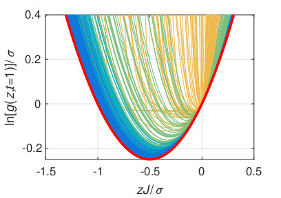
We observe numerically that these unicyclic asymmetric random walks are “optimal” in the sense that they minimize the generating function at any given $z$ and $t$ . Changing the rates non-uniformly and adding further cycles only increases the distance from the bound. In order to illustrate this observation, we show in Fig. 3 the effects of perturbations of the rate matrix of the type

k_{ij}=k^{+}\mathrm{e}^{\varepsilon\theta_{i}^{+}}\delta_{i,j+1}+k^{-}\mathrm{e}^{\varepsilon\theta_{i}^{-}}\delta_{i+1,j}+\varepsilon\phi_{ij},

(14)

where the $\theta_{i}$ are independently drawn from a standard normal distribution and the $\phi_{ij}$ are zero for $|i-j|\leq 1$ and exponentially distributed otherwise. While the terms with $\theta_{i}^{\pm}$ make the unicyclic rates non-uniform, the terms $\phi_{ij}$ add further cycles to the network. We calculate the generating function numerically for $t=1$ , which qualifies as an intermediate time scale for transition rates of order $1$ . The bound (11) is satisfied in all cases.

IV.3 Short-time and linear response limits

While a full proof of the parabolic bound (11) seems to be currently out of reach, we can prove a weaker bound, which becomes equivalent to (11) for small $t$ . We start with the fluctuation relation

p(-s_{\mathrm{tot}},-X,t)/p(s_{\mathrm{tot}},X,t)=\exp(-\stot)

(15)

for the joint probability distribution of the total entropy production and the current of interest at arbitrary time $t$ , which follows directly from the time reversal of the trajectories contributing to a fixed value of $s_{\mathrm{tot}}$ [3]. Using this relation, the generating function (7) can be written (dropping the index ‘tot’) as

	$\displaystyle g(z,t)$	$\displaystyle=\int\mathrm{d}s\int\mathrm{d}X\,p(s,X,t)\,\mathrm{e}^{zX}=\frac{1}{2}\left\langle\mathrm{e}^{zX}+\mathrm{e}^{-zX-s}\right\rangle$
		$\displaystyle=\left\langle\mathrm{e}^{-s/2}\cosh(zX+s/2)\right\rangle.$		(16)

Bounding the hyperbolic cosine by a parabola that touches it at $z=0$ and $z=-s/X$ , we obtain

$\displaystyle g(z,t)\geq$	$\displaystyle 1+\left\langle(1-\mathrm{e}^{-s})zX(1+zX/s)\right\rangle/2$
	$\displaystyle=1+zJt+z^{2}\sigma t\int_{0}^{\infty}\mathrm{d}s\int_{-\infty}^{\infty}\mathrm{d}X\psi(s,X)\,(X/s)^{2}$
	$\displaystyle\geq 1+tJz(1+zJ/\sigma).$	(17)

In the last step we have used Jensen’s inequality for the averages with the distribution $\psi(s,X)\equiv p(s,X,t)s(1-\mathrm{e}^{-s})/\sigma t$ for $s\geq 0$ , which is non-negative, normalized, and gives

\int_{0}^{\infty}\mathrm{d}s\int_{-\infty}^{\infty}\mathrm{d}X\psi(s,X)\,(X/s)=J/\sigma.

(18)

While the bound (17) is rigorous for arbitrary times $t$ , it is useful mainly for short times as a first order expansion of the otherwise stronger bound on $g(z,t)$ that follows from Eq. (11). Indeed, for the variance of the current, the bound (17) implies for arbitrary $t$

\left\langle X(t)^{2}\right\rangle\geq 2tJ^{2}/\sigma.

(19)

Equation (2) differs from this relation only by the term $\left\langle X(t)\right\rangle^{2}=J^{2}t^{2}$ and is thus proven for small times $t$ in linear order.

In the linear response regime for small driving affinity $\mathcal{A}$ , the current scales as $J\simeq\mathcal{A}$ and the entropy production rate as $\sigma\simeq\mathcal{A}^{2}$ . Hence the bound (19) implies Eq. (2) in the linear response limit for any fixed time, as follows from the scaling $J\sim\mathcal{A}$ and $\sigma\sim\mathcal{A}^{2}$ for small driving affinities $\mathcal{A}$ .

IV.4 Numerical check for intermediate times

On intermediate time scales we have verified the bound (11) numerically using a combination of random search and optimization techniques. At first, we have generated in total more than $3\times 10^{5}$ fully connected networks with $N\in\{3,4,5,7,10\}$ states and random transition rates with $\ln k_{ij}$ distributed uniformly between $-12$ and $5$ . A sample of such a network with $N=5$ states is illustrated in the inset of Fig. 4. For these networks we have calculated the stationary distribution and the generating function $g(z,t=1)$ via Eq. (7) with $Jz/\sigma$ ranging from $-2$ to $1$ . It is sufficient to check the bound for $t=1$ , since the large range of the choice of transition rates effectively covers different timescales. This procedure has been repeated for the currents of total entropy production ( $d_{ij}=d_{ij}^{\mathrm{s}}$ in Eq. (6)) and medium entropy production ( $d_{ij}=d_{ij}^{\mathrm{m}}$ ), as shown in Fig. 4, the current along an individual link $i\to j$ , and a current defined by a random asymmetric matrix $d_{ij}$ . Each of the random networks has then been used as a starting point for a constrained local minimization procedure that varies the rates $k_{ij}$ to minimize $g(z,t=1)$ while keeping $\sigma$ and $Jz/\sigma$ fixed (without this constraint the algorithm quickly finds the linear response regime, for which we have proven the validity of the bound). As Fig. 4 illustrates for a small set of networks, the bound (11) has proven valid for all of the random networks as well as for the optimized networks.

V Conclusion

We have shown that the thermodynamic uncertainty relation between the fluctuations of any current and the rate of entropy production in a NESS holds on arbitrary timescales. This result follows from a parabolic bound on the cumulant generating function associated with such a current. The fluctuation theorem for entropy production allows proving this bound in the limit of short timescales, complementing the previously known proof based on large deviation theory for the long-time limit. For intermediate timescales the bound is a conjecture that we have verified using extensive numerical checks. A full proof in this regime seems to call for new mathematical methods for the description of non-equilibrium steady states, which go beyond fluctuation theorems and large deviation theory.

For an experimental illustration in the case where the entropy production is measurable, we have analyzed this finite-time uncertainty relation with the work that is performed on a colloidal particle in a stochastically switching trap. As a next experimental step, it will be interesting to apply this relation to systems driven by chemical reactions like molecular motors, in order to bound the then a priori unknown rate of entropy production from below. Our generalization of the thermodynamic uncertainty relation should then become a valuable tool for inferring hidden thermodynamic properties of driven systems from experimental trajectories of finite length.

Note added: Recently, a proof of Eq. (2) for the special case $X=s_{\mathrm{tot}}$ and Langevin dynamics has been reported in a preprint [40].

Acknowledgements.

We thank Andre C. Barato for fruitful interactions on related projects.

References

[1] F. Ritort, “Single-molecule experiments in biological physics: Methods and applications,” J. Phys.: Condens. Matter 18, R531 (2006).
[2] S. Ciliberto, S. Joubaud, and A. Petrosyan, “Fluctuations in out-of-equilibrium systems: From theory to experiment,” J. Stat. Mech.: Theor. Exp., P12003 (2010).
[3] U. Seifert, “Stochastic thermodynamics, fluctuation theorems, and molecular machines,” Rep. Prog. Phys. 75, 126001 (2012).
[4] J. P. Pekola, “Towards quantum thermodynamics in electronic circuits,” Nature Phys. 11, 118 (2015).
[5] S. Gasparinetti, K. L. Viisanen, O.-P. Saira, T. Faivre, M. Arzeo, M. Meschke, and J. P. Pekola, “Fast electron thermometry for ultrasensitive calorimetric detection,” Phys. Rev. Applied 3, 014007 (2015).
[6] A. C. Barato and U. Seifert, “Thermodynamic uncertainty relation for biomolecular processes,” Phys. Rev. Lett. 114, 158101 (2015a).
[7] T. R. Gingrich, J. M. Horowitz, N. Perunov, and J. L. England, “Dissipation bounds all steady-state current fluctuations,” Phys. Rev. Lett. 116, 120601 (2016).
[8] H. Touchette, “The large deviation approach to statistical mechanics,” Phys. Rep. 478, 1 (2009).
[9] A. C. Barato and R. Chetrite, “A formal view on level 2.5 large deviations and fluctuation relations,” J. Stat. Phys. 160, 1154 (2015).
[10] P. Pietzonka, A. C. Barato, and U. Seifert, “Universal bounds on current fluctuations,” Phys. Rev. E 93, 052145 (2016a).
[11] T. R. Gingrich, G. M. Rotskoff, and J. M. Horowitz, “Inferring dissipation from current fluctuations,” J. Phys. A: Math. Theor. 50, 184004 (2017).
[12] P. Pietzonka, A. C. Barato, and U. Seifert, “Affinity- and topology-dependent bound on current fluctuations,” J. Phys. A: Math. Theor.49, 34LT01 (2016b).
[13] M. Polettini, A. Lazarescu, and M. Esposito, “Tightening the uncertainty principle for stochastic currents,” Phys. Rev. E 94, 052104 (2016).
[14] P. Tsobgni Nyawo and H. Touchette, “Large deviations of the current for driven periodic diffusions,” Phys. Rev. E 94, 032101 (2016).
[15] G. M. Rotskoff, “Mapping current fluctuations of stochastic pumps to nonequilibrium steady states,” Phys. Rev. E 95, 030101 (2017).
[16] J. P. Garrahan, “Simple bounds on fluctuations and uncertainty relations for first-passage times of counting observables,” Phys. Rev. E 95, 032134 (2017).
[17] A. C. Barato and U. Seifert, “Universal bound on the Fano factor in enzyme kinetics,” J. Phys. Chem. B 119, 6555 (2015b).
[18] G. Falasco, R. Pfaller, A. P. Bregulla, F. Cichos, and K. Kroy, “Exact symmetries in the velocity fluctuations of a hot brownian swimmer,” Phys. Rev. E 94, 030602 (2016).
[19] J. Guioth and D. Lacoste, “Thermodynamic bounds on equilibrium fluctuations of a global or local order parameter,” EPL 115, 60007 (2016).
[20] M. Nguyen and S. Vaikuntanathan, “Design principles for nonequilibrium self-assembly,” Proc. Natl. Acad. Sci. U.S.A. 113, 14231 (2016).
[21] A. C. Barato and U. Seifert, “Cost and precision of Brownian clocks,” Phys. Rev. X 6, 041053 (2016).
[22] P. Pietzonka, A. C. Barato, and U. Seifert, “Universal bound on the efficiency of molecular motors,” J. Stat. Mech.: Theor. Exp., 124004 (2016c).
[23] I. A. Martínez, E. Roldán, L. Dinis, D. Petrov, J. M. R. Parrondo, and R. A. Rica, “Brownian Carnot engine,” Nature Phys. 12, 67 (2016).
[24] C. Jarzynski, “Nonequilibrium equality for free energy differences,” Phys. Rev. Lett. 78, 2690 (1997).
[25] G. E. Crooks, “Entropy production fluctuation theorem and the nonequilibrium work relation for free energy differences,” Phys. Rev. E 60, 2721 (1999).
[26] D. Collin, F. Ritort, C. Jarzynski, S. Smith, I. Tinoco, and C. Bustamante, “Verification of the Crooks fluctuation theorem and recovery of RNA folding free energies,” Nature 437, 231 (2005).
[27] U. Seifert, “Entropy production along a stochastic trajectory and an integral fluctuation theorem,” Phys. Rev. Lett. 95, 040602 (2005).
[28] J. L. Lebowitz and H. Spohn, “A Gallavotti-Cohen-type symmetry in the large deviation functional for stochastic dynamics,” J. Stat. Phys. 95, 333 (1999).
[29] T. Speck, V. Blickle, C. Bechinger, and U. Seifert, “Distribution of entropy production for a colloidal particle in a nonequilibrium steady state,” EPL 79, 30002 (2007).
[30] J. R. Gomez-Solano, L. Bellon, A. Petrosyan, and S. Ciliberto, “Steady-state fluctuation relations for systems driven by an external random force,” EPL 89, 60003 (2010).
[31] E. Dieterich, J. Camunas-Soler, M. Ribezzi-Crivellari, U. Seifert, and F. Ritort, “Single-molecule measurement of the effective temperature in non-equilibrium steady states,” Nature Phys. 11, 971 (2015).
[32] S.-W. Wang, K. Kawaguchi, S.-i. Sasa, and L.-H. Tang, “Entropy production of nanosystems with time scale separation,” Phys. Rev. Lett. 117, 070601 (2016).
[33] V. Blickle and C. Bechinger, “Realization of a micrometre-sized stochastic heat engine,” Nature Phys. 8, 143 (2012).
[34] K. Visscher, M. Schnitzer, and S. M. Block, “Single kinesin molecules studied with a molecular force clamp,” Nature 400, 184 (1999).
[35] J. M. Schurr and B. S. Fujimoto, “Equalities for the nonequilibrium work transferred from an external potential to a molecular system. Analysis of single-molecule extension experiments,” J. Phys. Chem. B 107, 14007 (2003).
[36] A. Mossa, S. de Lorenzo, J. M. Huguet, and F. Ritort, “Measurement of work in single-molecule pulling experiments,” J. Chem. Phys. 130, 234116 (2009).
[37] F. Ritort, “Work and heat fluctuations in two-state systems: A trajectory thermodynamics formalism,” J. Stat. Mech.: Theor. Exp., P10016 (2004).
[38] K. Funo, T. Shitara, and M. Ueda, “Work fluctuation and total entropy production in nonequilibrium processes,” Phys. Rev. E 94, 062112 (2016).
[39] Even though the distribution of work $W_{2}$ often looks Gaussian in our experimental case study (see Fig. 2), the generating function would in these cases not be parabolic due to non-Gaussian tails of the distribution. Accordingly, the uncertainty relation is not saturated.
[40] S. Pigolotti, I. Neri, É. Roldán, and F. Jülicher, “Generic properties of stochastic entropy production,” arXiv:1704.04061 (2017).