跳到论文正文
W Papers独立论文阅读器 arXiv:1702.07393 论文正文 计算阅读时间 · 0%
引用这篇论文根据当前论文元数据生成,正式投稿前建议核对。


License: arXiv.org perpetual non-exclusive license
arXiv:1702.07393v4 [cs.RO] 22 Jan 2019

Controlling Parent Systems Through Swarms Using Abstraction

Kyle L. Crandall    and Adam M. Wickenheiser ††thanks: K.L. Crandall is with the Department of Mechanical and Aerospace Engineering, The George Washington University, Washington, DC, 20052 USA e-mail: crandallk@gwu.edu.††thanks: A.M. Wickenheiser is with The University of Delaware.††thanks: Manuscript received May 13, 2018; revised Jan. 18, 2019.
Abstract

This study considers the control of parent-child systems where a parent system is acted on by a set of controllable child systems (i.e. a swarm). Examples of such systems include a swarm of robots pushing an object over a surface, a swarm of aerial vehicles carrying a large load, or a set of end effectors manipulating an object. In this paper, a general approach for decoupling the swarm from the parent system through a low-dimensional abstract state space is presented. The requirements of this approach are given along with how constraints on both systems propagate through the abstract state and impact the requirements of the controllers for both systems. To demonstrate, several controllers with hard state constraints are designed to track a given desired angle trajectory of a tilting plane with a swarm of robots driving on top. Both homogeneous and heterogeneous swarms of varying sizes and properties are considered to test the robustness of this architecture. The controllers are shown to be locally asymptotically stable and are demonstrated in simulation.

Index Terms: 
Swarms, Adaptive Control, Cascaded Systems, Robust Control.

I Introduction

The appeal of using multiple, cooperating agents to perform complicated tasks has been demonstrated in many applications [1]. For example, when compared to a single robot, swarms can be designed to be more robust to failure, can take advantage of the inherent high degree of parallelism, and tend to be more economical with regard to reusability, maintenance, and scalability.

We consider a class of robot swarms that use multiple agents to affect a parent dynamical system. While there are many examples of this type of system being considered, there has not been much work studying the problem as a general case of backstepping-like control; however, there do exist some frequently cited approaches such as caging. This is where the swarm is arranged in such a way as to constrain the possible movement of the parent system. This approach is particularly common in the case where a swarm of ground robots is manipulating a larger, passive object over a 2D surface. Prior work has achieved caging by estimating the geometry of the object using contact with the swarm [2], or by exploiting a priori knowledge of the geometry [3]. This knowledge can also be utilized to define a set of high-level behaviors for the swarm that can be achieved in a decentralized manner [4]. Robots can even be linked together to exert more force [5]. These caging approaches assume passive parent systems with at least marginally stable dynamics that are not incorporated into the design of the swarm behavior. This precludes the evaluation of these methods’ ability to handle disturbances or complex parent system dynamics.

Another similar object manipulation problem is using a swarm of multirotors to carry an object. This can be approached using optimization, resulting in a feed forward controller based on full state feedback that takes into account a more complex model of the payload [6], or by breaking the problem into a path following problem and a coordination problem [7], resulting in a method similar to the caging methods discussed previously. Both of these approaches isolate the dynamics of an individual member of the swarm and determine how it needs to move, either with the rest of the swarm or relative to the parent system.

This parent-child class of system we are considering includes other cases that would not traditionally be considered “swarm” problems, such as a walking robot, where the legs could be considered a swarm manipulating the body [8]. An array of control surfaces could be considered a swarm acting on the wing of an aircraft [9] or bridge [10]. These problems are particularly challenging due to fluid-structure interactions with the parent systems. In these cases, caging methods as discussed earlier would be much more difficult to apply. While decentralized controllers for walking robots have been proposed [8], the controllers for the arrays of flaps controlling the aerodynamics are both centralized approaches that require each element of the swarm to know the states of all the other elements.

In this study, we propose a general approach to designing controllers for this type of parent-child system. This approach encapsulates the coupling between the dynamics of the parent and swarm systems within a lower-dimensional abstract state and the dynamics between the swarm and the abstract state within an auxiliary abstract state. This creates a cascaded system to which we can apply a backstepping controller. Specifically, we can design a controller for the parent system that specifies a desired abstract state of the swarm and a controller for the swarm that achieves the desired abstract state. Due to the nature of the abstract state, this isolates the swarm and parent systems, allowing for a large degree of flexibility in the swarm size and composition at runtime. While a centralized observer calculates the abstract states, the dimensionality of this estimation is fixed with respect to the size of the swarm. Additionally, the response of the parent system can be used to estimate the abstract state, eliminating the need to sense and estimate it directly.

The proposed approach relies on finding an abstract state of the swarm similar to the shape parameters used in formation control [11, 12, 13, 14, 15, 16, 17, 18]. This body of work uses a low-dimensional abstraction of a swarm of robots to describe the overall geometry of the swarm. For motion planning, this allows the distribution of the swarm to be specified rather than individual trajectories. These studies consider only the swarm, however, and do not possess a parent system with which to interact. Our method utilizes an abstraction depending on these interactions, facilitating the design of the swarm behavior based on the desired behavior of the parent system.

This paper formalizes the approach presented in [19] and considers constraints on the parent and swarm systems. In section II, we formally define the parent-swarm class of problem and our proposed approach and examine the stability of the system under constraints. In section III we present an example case, and we discuss simulation results in section IV.

II Method

Refer to caption
Fig. 1: Block Diagram depicting the the overall approach we are proposing

We propose to control a parent-child system by finding an abstraction of the swarm’s state that embodies the dynamic interactions between these two systems. Such a system is so called because it can be reasonably segregated into two cascading systems: the parent system and a swarm of child systems. The overall system must have the following properties:

  • •

    The parent system must contain the state that we seek to control.

  • •

    The parent system’s dynamics must be a function of the swarm’s state.

  • •

    The swarm’s interaction with the parent system must be modular in way that it can be broken into a variable number of child systems.

  • •

    The swarm’s dynamics must be a function of the inputs to the system.

The typical dynamics for such a system are governed by the following:

𝐱˙p=fp​(𝐱p,𝐱s,𝐮s),\displaystyle\dot{\mathbf{x}}_{p}=f_{p}\left(\mathbf{x}_{p},\mathbf{x}_{s},\mathbf{u}_{s}\right), where​fp:Xp×Xs×Us→T​Xp\displaystyle\ \textrm{where}\ f_{p}:X_{p}\times X_{s}\times U_{s}\rightarrow TX_{p} (1)
𝐱˙s=fs​(𝐱s,𝐮s),\displaystyle\dot{\mathbf{x}}_{s}=f_{s}\left(\mathbf{x}_{s},\mathbf{u}_{s}\right), where​fs:Xs×Us→T​Xs\displaystyle\ \textrm{where}\ f_{s}:X_{s}\times U_{s}\rightarrow TX_{s} (2)
𝐱˙s​i=fs​i​(𝐱s,𝐮s​i),\displaystyle\dot{\mathbf{x}}_{si}=f_{si}\left(\mathbf{x}_{s},\mathbf{u}_{si}\right), where​fs​i:Xs×Us​i→T​Xs​i\displaystyle\ \textrm{where}\ f_{si}:X_{s}\times U_{si}\rightarrow TX_{si} (3)

Here, 𝐱p\mathbf{x}_{p} is the state of the parent system, 𝐱s\mathbf{x}_{s} is the state of the swarm system, and 𝐱s​i\mathbf{x}_{si} is the state of the iith child system in the swarm. We can define the spaces these states exist in as 𝐱p∈Xp⊂ℝn\mathbf{x}_{p}\in X_{p}\subset\mathbb{R}^{n}, 𝐱s​i∈Xs​i⊂ℝmi\mathbf{x}_{si}\in X_{si}\subset\mathbb{R}^{m_{i}}, and 𝐱s∈Xs=∏i=1NXs​i\mathbf{x}_{s}\in X_{s}=\prod_{i=1}^{N}X_{si} where nn is the dimension of the parent state, mim_{i} is the dimension of the iith child’s state, and NN is the size of the swarm. 𝐮s\mathbf{u}_{s} is the input to the system and is a concatenation of inputs 𝐮s​i\mathbf{u}_{si}, which are the inputs to the iith child. Thus, 𝐮s​i∈Us​i⊂ℝpi\mathbf{u}_{si}\in U_{si}\subset\mathbb{R}^{p_{i}} and 𝐮s∈Us=∏i=1NUs​i\mathbf{u}_{s}\in U_{s}=\prod_{i=1}^{N}U_{si}. The notation T​XpTX_{p} and T​XsTX_{s} denote the tangent space of XpX_{p} and XsX_{s} respectively.

Figure 1 is a diagram of the overall architecture of the proposed approach. Note that it is similar to a backstepping architecture, where the controller of the parent system specifies a desired intermediate state, and then the controller on the swarm uses that desired intermediate state to calculate how it should move to achieve it. The innovation of our proposal is the introduction of the abstract state based on the interactions between the swarm and parent systems, allowing the dynamics of the swarm that are of little consequence to the parent system to be truncated.

II-A Abstraction of the Swarm

The crux of our approach is the idea of abstracting the complex interactions of the swarm and the parent systems. This idea is based on work by Belta and Kumar, where they propose using abstraction to control formations of robots [11]. They find an abstract state of the swarm that represents the formation’s geometric properties such as position, orientation, and distribution. Rather than specifying states that necessarily define the geometric features of the swarm, we use states that encompass the coupling dynamics between the swarm and the parent system.

Definition II.1 (Abstraction of a Swarm with Respect to a Parent System).

An abstraction of the swarm is a mapping from the state of the swarm to an abstract state that encapsulates all the interactions between the swarm and the parent systems as described below in (6). The dimension of this abstract state must be independent of the number of child systems in the swarm.

This abstraction consists of an abstract state 𝐚∈A⊂ℝm\mathbf{a}\in A\subset\mathbb{R}^{m}, and a mapping from the swarm state to the abstract state:

𝐚=ϕ⁡(𝐱s,𝐮s)​where​ϕ:Xs×Us→A\mathbf{a}=\phi\left(\mathbf{x}_{s},\mathbf{u}_{s}\right)\ \textrm{where}\ \phi:X_{s}\times U_{s}\rightarrow A (4)

This mapping must be surjective, i.e. every abstract state must represent at least one swarm state. We further require the dynamics of the parent system to be rewritten as

𝐱˙p=f^p​(𝐱p,𝐚),where​f^p:Xp×A→T​Xp\dot{\mathbf{x}}_{p}=\hat{f}_{p}\left(\mathbf{x}_{p},\mathbf{a}\right),\ \textrm{where}\ \hat{f}_{p}:X_{p}\times A\rightarrow TX_{p} (5)

and fpf_{p} is a composition of f^p\hat{f}_{p} and ϕ\phi:

fp​(𝐱p,𝐱s,𝐮s)=f^p​(𝐱p,ϕ⁡(𝐱s,𝐮s))f_{p}\left(\mathbf{x}_{p},\mathbf{x}_{s},\mathbf{u}_{s}\right)=\hat{f}_{p}\left(\mathbf{x}_{p},\phi\left(\mathbf{x}_{s},\mathbf{u}_{s}\right)\right) (6)

Since the dynamics of the parent state can be framed as dependent on this abstract state, the abstract state can be estimated based on the response of the parent system. This allows for the estimation of the abstract state without a global observer, though one can still be used.

Once an abstraction of the swarm has been found, we can design a control law for the parent system in which the abstract state is considered to be the input and the swarm is considered to be independent of the parent (which follows from (3)). In general, the swarm control law is a function of the parent and swarm states, i.e. 𝐮s=𝐮s​(𝐱p,𝐱s)\mathbf{u}_{s}=\mathbf{u}_{s}(\mathbf{x}_{p},\mathbf{x}_{s}). We can rewrite this relationship in terms of the abstract state as follows:

𝐮s=𝐮s​(𝐚,𝐚d,𝐚a​u​x)\mathbf{u}_{s}=\mathbf{u}_{s}(\mathbf{a},\mathbf{a}_{d},\mathbf{a}_{aux}) (7)

where 𝐚d\mathbf{a}_{d} is the desired abstract state as determined by the parent controller, and 𝐚a​u​x\mathbf{a}_{aux} is the auxiliary abstract state, which collects the remaining terms in the control law.

Definition II.2 (Auxiliary Abstraction of the Swarm).

Given an abstract state 𝐚\mathbf{a} from Definition II.1, an Auxiliary Abstract State 𝐚a​u​x\mathbf{a}_{aux} embodies the interactions within the swarm in its control law.

The auxiliary abstract state 𝐚a​u​x∈Aa​u​x⊂ℝma​u​x\mathbf{a}_{aux}\in A_{aux}\subset\mathbb{R}^{m_{aux}} is mapped from the full swarm state 𝐚a​u​x=ϕa​u​x​(𝐱s)\mathbf{a}_{aux}=\phi_{aux}\left(\mathbf{x}_{s}\right), where ϕa​u​x:Xs→Aa​u​x\phi_{aux}:X_{s}\rightarrow A_{aux}.

II-B Constraint Considerations for Controller Design

Any constraints on the parent and swarm systems must also be considered in the abstraction. To do this, let Xs​c⊆XsX_{sc}\subseteq X_{s} be the set of all swarm states that satisfy all constraints. Because the abstract mapping is not necessarily injective, a given abstract state can correspond to a set of swarm states, some of which may lie outside Xs​cX_{sc}. Thus, we partition the set of abstract states into three disjoint sets: absolutely constrained abstract states, partially constrained abstract states, and unconstrained abstract states.

Definition II.3 (Absolutely Constrained Abstract State).

An abstract state is said to be absolutely constrained if the set it maps to in the swarm state space exists entirely within the constraints on the swarm. The set of all absolutely constrained abstract states is the set AA={𝐚∈A|ϕ−1​[𝐚]⊆Xs​c}A_{A}=\left\{\mathbf{a}\in A\ |\ \phi^{-1}\left[\mathbf{a}\right]\subseteq X_{sc}\right\}.

Definition II.4 (Unconstrained Abstract State).

An abstract state is said to be unconstrained if the set it maps to in the swarm state violates at least one constraint on the swarm state at all points. The set of all unconstrained abstract states is the set AU={𝐚∈A|ϕ−1​[𝐚]⊆Xs∖Xs​c}A_{U}=\left\{\mathbf{a}\in A\ |\ \phi^{-1}\left[\mathbf{a}\right]\subseteq X_{s}\setminus X_{sc}\right\}.

Definition II.5 (Partially Constrained Abstract State).

An abstract state is said to be partially constrained if the set it maps to in the swarm state violates any of the constraints on the swarm at some points, but not all points. The set of all partially constrained abstract states is thus AP=A∖(AA∪AU)A_{P}=A\setminus\left(A_{A}\cup A_{U}\right)

We choose a domain ACA_{C} on which we constrain the abstract state.

AC⊆AA∪APA_{C}\subseteq A_{A}\cup A_{P} (8)

If AC⊆AAA_{C}\subseteq A_{A}, the swarm controller does not have to consider the swarm constraints since all configurations of the swarm that correspond to that abstract state satisfy the constraints on the swarm. If AC∩AP≠∅A_{C}\cap A_{P}\neq\emptyset, the swarm controller must ensure that it drives the swarm to a configuration that does not violate the constraints on the swarm.

II-C Stability

Given Lyapunov functions for the parent and swarm subsystems, we can derive sufficient conditions for the stability of the closed loop system. The closed-loop system is broken into two parts: 𝐱˙p=fp′​(𝐱p)\dot{\mathbf{x}}_{p}=f_{p}^{\prime}\left(\mathbf{x}_{p}\right) is the closed-loop parent system, and 𝐚˙=fa′​(𝐚)\dot{\mathbf{a}}=f_{a}^{\prime}\left(\mathbf{a}\right) is the closed-loop swarm system in the abstract space. First, we consider the stability of systems without constraints.

Theorem 1.

Consider the following systems:

𝐱˙p=fp′​(𝐱p)\dot{\mathbf{x}}_{p}=f_{p}^{\prime}\left(\mathbf{x}_{p}\right) (9)
𝐚˙=fa′​(𝐚)\dot{\mathbf{a}}=f_{a}^{\prime}\left(\mathbf{a}\right) (10)

Let Vp​(𝐱p)V_{p}\left(\mathbf{x}_{p}\right) be a Lyapunov candidate for the parent system, and let Va​(𝐚)V_{a}\left(\mathbf{a}\right) be a Lyapunov candidate for the abstract system. Let 𝐱pT=[𝐳pT𝐲pT]\mathbf{x}_{p}^{T}=\begin{bmatrix}\mathbf{z}_{p}^{T}&\mathbf{y}_{p}^{T}\end{bmatrix} and 𝐚T=[𝐳aT𝐲aT]\mathbf{a}^{T}=\begin{bmatrix}\mathbf{z}_{a}^{T}&\mathbf{y}_{a}^{T}\end{bmatrix} be partitioned such that

V˙p≤V˙p′​(𝐳p)+V˙p​c​(𝐳p,𝐳a)\dot{V}_{p}\leq\dot{V}_{p}^{\prime}\left(\mathbf{z}_{p}\right)+\dot{V}_{pc}\left(\mathbf{z}_{p},\mathbf{z}_{a}\right) (11)
V˙a≤V˙a′​(𝐳a)+V˙a​c​(𝐳p,𝐳a)\dot{V}_{a}\leq\dot{V}_{a}^{\prime}\left(\mathbf{z}_{a}\right)+\dot{V}_{ac}\left(\mathbf{z}_{p},\mathbf{z}_{a}\right) (12)

with domains 𝐳p∈Dz​p\mathbf{z}_{p}\in D_{zp}, 𝐳a∈Dz​a\mathbf{z}_{a}\in D_{za}, 𝐲p∈Dy​p\mathbf{y}_{p}\in D_{yp} and 𝐲a∈Dy​a\mathbf{y}_{a}\in D_{ya}. The terms V˙p′\dot{V}^{\prime}_{p} and V˙a′\dot{V}^{\prime}_{a} represent the terms of V˙p\dot{V}_{p} and V˙a\dot{V}_{a} that are solely dependent on the parent and abstract states, respectively. The terms V˙p​c\dot{V}_{pc} and V˙a​c\dot{V}_{ac} represent the coupled terms. Note that any of these terms can be 00, i.e. the systems may not be coupled, or the coupling may be in one direction.

If V˙p′\dot{V}_{p}^{\prime} and V˙a′\dot{V}_{a}^{\prime} are negative definite, and

|V˙p′+V˙a′|>|V˙p​c+V˙a​c|\left|\dot{V}_{p}^{\prime}+\dot{V}_{a}^{\prime}\right|>\left|\dot{V}_{pc}+\dot{V}_{ac}\right| (13)

when 𝐳p∈Dz​p∖{0},𝐳a∈Dz​a∖{0}\mathbf{z}_{p}\in D_{zp}\setminus\left\{0\right\},\ \mathbf{z}_{a}\in D_{za}\setminus\left\{0\right\}, and

|V˙p​c​(0,0)+V˙a​c​(0,0)|=0,\left|\dot{V}_{pc}\left(0,0\right)+\dot{V}_{ac}\left(0,0\right)\right|=0, (14)

then the origin of this system is locally stable with a region of attraction in the neighborhood of the origin such that if [𝐳pT𝐳aT𝐲pT𝐲aT]T∈S⊂Dz​p×Dz​a×Dy​p×Dy​a\begin{bmatrix}\mathbf{z}_{p}^{T}&\mathbf{z}_{a}^{T}&\mathbf{y}_{p}^{T}&\mathbf{y}_{a}^{T}\end{bmatrix}^{T}\in S\subset D_{zp}\times D_{za}\times D_{yp}\times D_{ya}, then 𝐳p→0\mathbf{z}_{p}\to 0 and 𝐳a→0\mathbf{z}_{a}\to 0 as t→∞t\to\infty and 𝐲p\mathbf{y}_{p} and 𝐲a\mathbf{y}_{a} remain bounded.

Proof.

Let V⁡(𝐳p,𝐲p,𝐳a,𝐲a)=Vp​(𝐳p,𝐲p)+Va​(𝐳a,𝐲a)V\left(\mathbf{z}_{p},\mathbf{y}_{p},\mathbf{z}_{a},\mathbf{y}_{a}\right)=V_{p}\left(\mathbf{z}_{p},\mathbf{y}_{p}\right)+V_{a}\left(\mathbf{z}_{a},\mathbf{y}_{a}\right). Because VpV_{p} and VaV_{a} are positive definite, VV is also positive definite.

We now take the derivative of VV with respect to time:

V˙≤V˙p′​(𝐳p)+V˙a′​(𝐳a)+V˙p​c​(𝐳p,𝐳a)+V˙a​c​(𝐳p,𝐳a)≤−|V˙p′​(𝐳p)+V˙a′​(𝐳a)|+|V˙p​c​(𝐳p,𝐳a)+V˙a​c​(𝐳p,𝐳a)|\dot{V}\leq\dot{V}_{p}^{\prime}\left(\mathbf{z}_{p}\right)+\dot{V}_{a}^{\prime}\left(\mathbf{z}_{a}\right)+\dot{V}_{pc}\left(\mathbf{z}_{p},\mathbf{z}_{a}\right)+\dot{V}_{ac}\left(\mathbf{z}_{p},\mathbf{z}_{a}\right)\leq-\left|\dot{V}_{p}^{\prime}\left(\mathbf{z}_{p}\right)+\dot{V}_{a}^{\prime}\left(\mathbf{z}_{a}\right)\right|+\left|\dot{V}_{pc}\left(\mathbf{z}_{p},\mathbf{z}_{a}\right)+\dot{V}_{ac}\left(\mathbf{z}_{p},\mathbf{z}_{a}\right)\right| (15)

Therefore, for V˙\dot{V} to be negative semi-definite,

|V˙p′+V˙a′|≥|V˙p​c+V˙a​c|\left|\dot{V}_{p}^{\prime}+\dot{V}_{a}^{\prime}\right|\geq\left|\dot{V}_{pc}+\dot{V}_{ac}\right| (16)

Next, we find where V˙=0\dot{V}=0. This should only be true at the origin to satisfy the Lyapunov stability theorem (Theorem 4.1, [20]); therefore, we determine that, for 𝐳p≠0\mathbf{z}_{p}\neq 0 and 𝐳a≠0\mathbf{z}_{a}\neq 0,

|V˙p′​(𝐳p)+V˙a′​(𝐳a)|≠|V˙p​c​(𝐳p,𝐳a)+V˙a​c​(𝐳p,𝐳a)|\left|\dot{V}_{p}^{\prime}\left(\mathbf{z}_{p}\right)+\dot{V}_{a}^{\prime}\left(\mathbf{z}_{a}\right)\right|\neq\left|\dot{V}_{pc}\left(\mathbf{z}_{p},\mathbf{z}_{a}\right)+\dot{V}_{ac}\left(\mathbf{z}_{p},\mathbf{z}_{a}\right)\right| (17)

This combined with (16) gives us the inequality in (13).

Finally, we consider 𝐳p=0\mathbf{z}_{p}=0 and 𝐳a=0\mathbf{z}_{a}=0, which gives us (14). Given these conditions, we can say that V˙\dot{V} is negative semi-definite on the domain D=Dp×Da×ℝd​i​m​(𝐲p)×ℝd​i​m​(𝐲p)D=D_{p}\times D_{a}\times\mathbb{R}^{dim\left(\mathbf{y}_{p}\right)}\times\mathbb{R}^{dim\left(\mathbf{y}_{p}\right)}. Thus, by Theorem 8.4 in [20], the terms 𝐳p\mathbf{z}_{p} and 𝐳a\mathbf{z}_{a} are asymptotically stable with the region of attraction

S={𝐳∈D|V⁡(𝐳)≤min⁡{V⁡(𝐛)|𝐛∈b​d​(D)}}S=\left\{\mathbf{z}\in D\ |\ V\left(\mathbf{z}\right)\leq\min\left\{V\left(\mathbf{b}\right)|\mathbf{b}\in bd\left(D\right)\right\}\right\} (18)

while 𝐲p\mathbf{y}_{p} and 𝐲a\mathbf{y}_{a} remain bounded; thus, SS is a closed neighborhood of the origin. Note that b​d​(D)bd\left(D\right) is the boundary of the set DD. ∎

Remark.

Let ϕ⁡(𝐱s)\phi\left(\mathbf{x}_{s}\right) be an abstraction of 𝐱s\mathbf{x}_{s}. If ϕ−1​[Dz​a]\phi^{-1}\left[D_{za}\right] is bounded, where Dz​aD_{za} is defined as in Theorem 1, then the swarm state is also bounded. However, if this inverse mapping from an abstract state is unbounded, then we cannot make any inference about the boundedness of the swarm state based on the boundedness of the abstract state.

We can now consider how the constraints on the system affect the region of attraction of the system.

Theorem 2.

Consider a parent-child system with constrained spaces Xp​cX_{pc} and Xs​cX_{sc} for the parent and swarm states, respectively, and let ACA_{C} be a constrained abstract space that contains the origin. Let Ad⊆ACA_{d}\subseteq A_{C} be a region in which the desired abstract state is further constrained. Let 𝐰p​(t)=[𝐳pT​(t)𝐲pT​(t)]T\mathbf{w}_{p}\left(t\right)=\begin{bmatrix}\mathbf{z}_{p}^{T}\left(t\right)&\mathbf{y}_{p}^{T}\left(t\right)\end{bmatrix}^{T} and 𝐰𝐚​(t)=[𝐳aT​(t)𝐲aT​(t)]T\mathbf{w_{a}}\left(t\right)=\begin{bmatrix}\mathbf{z}_{a}^{T}\left(t\right)&\mathbf{y}_{a}^{T}\left(t\right)\end{bmatrix}^{T} be trajectories in the parent and abstract spaces that satisfy the conditions of Theorem 1. Let Dp=Dz​p×Dy​pD_{p}=D_{zp}\times D_{yp} and Da=Dz​a×Dy​aD_{a}=D_{za}\times D_{ya}. If there exist nonempty sets

Dp​c={𝐰p∈Dp|𝐱p​d(t)+𝐛‖𝐰p‖∈Xp​c,∀t∈[0,∞),𝐛∈Bd​i​m​(Xp)}D_{pc}=\left\{\mathbf{w}_{p}\in D_{p}\ |\ \mathbf{x}_{pd}\left(t\right)+\mathbf{b}\left\lVert\mathbf{w}_{p}\right\rVert\in X_{pc},\forall\ t\in\left[0,\infty\right),\mathbf{b}\in B^{dim\left(X_{p}\right)}\right\} (19)
Da​c={𝐰a∈Da|𝐚d+𝐛‖𝐰a‖∈AC,∀𝐚d∈Ad,𝐛∈Bd​i​m​(A)}D_{ac}=\left\{\mathbf{w}_{a}\in D_{a}\ |\ \mathbf{a}_{d}+\mathbf{b}\left\lVert\mathbf{w}_{a}\right\rVert\in A_{C},\ \forall\ \mathbf{a}_{d}\in A_{d},\mathbf{b}\in B^{dim\left(A\right)}\right\} (20)

where

Bn={𝐯∈ℝn|‖𝐯‖=1}B^{n}=\left\{\mathbf{v}\in\mathbb{R}^{n}\ |\ \left\lVert\mathbf{v}\right\rVert=1\right\} (21)

and 𝐱p​d​(t)\mathbf{x}_{pd}\left(t\right) is the desired trajectory of the parent state, then there exists a nonempty domain ScS_{c} on which the origin of the system is asymptotically stable and Dp​cD_{pc} and Da​cD_{ac} are forward time-invariant for all future time, where ScS_{c} is given by

Sc={𝐳∈S∩Dc|Vp​(𝐳)+Va​(𝐳)≤min⁡{Vp​(𝐛)+Va​(𝐛)∣b∈b​d​(S∩Dc)}}S_{c}=\left\{\mathbf{z}\in S\cap D_{c}\ |\ V_{p}\left(\mathbf{z}\right)+V_{a}\left(\mathbf{z}\right)\leq\min\left\{V_{p}\left(\mathbf{b}\right)+V_{a}\left(\mathbf{b}\right)\mid b\in bd\left(S\cap D_{c}\right)\right\}\right\} (22)

and Dc=Dp​c×Da​c×ℝd​i​m​(𝐲p)×ℝd​i​m​(𝐲a)D_{c}=D_{pc}\times D_{ac}\times\mathbb{R}^{dim\left(\mathbf{y}_{p}\right)}\times\mathbb{R}^{dim\left(\mathbf{y}_{a}\right)}

Proof.
Refer to caption
Fig. 2: Diagram of the sets defined in Theorems 1 and 2. SS is the region of attraction of the origin of (9) and (10), DcD_{c} is the subset of additive perturbation vectors that do not violate any constraints, and ScS_{c} is the maximal set of contours of V⁡(𝐳)V\left(\mathbf{z}\right) contained within S∩DcS\cap D_{c}.

Let 𝐳p×𝐳a×𝐲p×𝐲a∈Sc\mathbf{z}_{p}\times\mathbf{z}_{a}\times\mathbf{y}_{p}\times\mathbf{y}_{a}\in S_{c}. Then 𝐳p∈Dp​c\mathbf{z}_{p}\in D_{pc}, and so 𝐱p​d​(t)+𝐛⁡‖𝐳p‖∈Xp\mathbf{x}_{pd}\left(t\right)+\mathbf{b}\left\lVert\mathbf{z}_{p}\right\rVert\in X_{p}. By Theorem 1, 𝐳p\mathbf{z}_{p} and 𝐳a\mathbf{z}_{a} converge to 0 asymptotically with a region of attraction SS. By Theorem 8.4 in [20], if 𝐳0∈Sc\mathbf{z}_{0}\in S_{c}, then V⁡(𝐳⁡(t))→0V\left(\mathbf{z}\left(t\right)\right)\rightarrow 0 and hence 𝐳⁡(t)∈Sc\mathbf{z}\left(t\right)\in S_{c} as t→∞t\rightarrow\infty. The relationships between these sets are illustrated in figure 2.

The sets Dp​cD_{pc} and Da​cD_{ac} contain the origin since it is assumed that the desired trajectory of the parent system is feasible. SS is the semilevel set of a positive definite Lyapunov function; therefore, the intersection S∩DcS\cap D_{c} must contain the origin. The set ScS_{c} is also a semilevel set of the same Lyapunov function, so it must also contain the origin. Therefore, as long as the desired trajectory and desired abstract surface satisfy all constraints, the set ScS_{c} at least contains the origin. ∎

Using these two theorems, we can build a stability proof for the whole system based on the individual Lyapunov functions for the controllers for the parent and swarm systems. We can define a region of attraction that satisfies all constraints by mapping the constraints on the separate subsystems. Note that if the system is not globally asymptotically stable, the estimate of the region of attraction tends to be quite conservative, which is exacerbated in the presence of constraints. The key point to these theorems however lies in equation (13), which states that the stability of the overall closed-loop system is dependent on the coupling terms in the Lyapunov candidate being dominated by the non-coupling terms.

III Example Case
Refer to caption
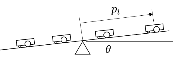
Fig. 3: Diagram of example system. The generalized coordinates are shown and labeled. θ\theta is the angle the tilting plane makes with the ground, and pip_{i} is the distance robot ii is from the axis of rotation of the plane.

One of the key advantages of the system we propose is its modularity. We demonstrate this by developing two different controllers for an example parent system based on techniques pulled from the literature and likewise swarm controllers for two different swarms. We present simulation results of various combinations of these systems and controllers to demonstrate the modularity of this approach. We show that the designed controllers can be used interchangeably, and that similar results for a given parent system controller can be achieved by any size of the two swarms considered, as well as by heterogeneous swarms consisting of members of both types of swarm.

To demonstrate our proposed controller architecture, we have chosen to apply it to a swarm of robots driving on top of a tilting plane. Our controller drives the robots to balance the plane at a desired angle or track a desired tilt angle trajectory. Figure 3 is a diagram of the proposed system. θ\theta is the angle the surface of the tilting plane makes with the ground, and pip_{i} is the position of robot ii in the plane’s coordinate system, where pi=0p_{i}=0 at the axis of rotation of the plane. Robot ii has mass mim_{i}. The robots are constrained to move in lanes to avoid collisions with each other; this is effective as the plane is only allowed to tilt about one axis. This system was selected as it is simple enough to be easily modeled, and it demonstrates the advantages of our approach, yet it is complex enough that a control solution is not trivial.

In this system, the swarm is the group of NN robots driving on the plane, and the parent system is the plane itself. To examine the interactions between the parent and swarm systems, we state the equation of motion of the parent system:

(J+∑i=1Nmi​pi2)​θ¨+g​cos⁡(θ)​∑i=1Nmi​pi+2​θ˙​∑i=1Nmi​pi​p˙i+ff​(θ˙)=0\left(J+\displaystyle\sum_{i=1}^{N}m_{i}p^{2}_{i}\right)\ddot{\theta}+g\cos\left(\theta\right)\displaystyle\sum_{i=1}^{N}m_{i}p_{i}+2\dot{\theta}\displaystyle\sum_{i=1}^{N}m_{i}p_{i}\dot{p}_{i}+f_{f}\left(\dot{\theta}\right)=0 (23)

where JJ is the plane’s moment of inertia about its axis, ff​(θ˙)f_{f}\left(\dot{\theta}\right) is the Stribeck friction on the axis of rotation, and gg is the acceleration due to gravity.

Given these dynamics, we can identify the terms that embody the interaction between the parent system and the swarm. We choose the abstract state given in (24) and rewrite the dynamics of the parent system in terms of this state in (25):

𝐚=[τsJsJ˙s]=[g​∑i=1Nmi​pi∑i=1Nmi​pi2∑i=1N2​mi​pi​vi]T\mathbf{a}=\begin{bmatrix}\tau_{s}\\ J_{s}\\ \dot{J}_{s}\end{bmatrix}=\begin{bmatrix}g\displaystyle\sum_{i=1}^{N}m_{i}p_{i}&\displaystyle\sum_{i=1}^{N}m_{i}p_{i}^{2}&\displaystyle\sum_{i=1}^{N}2m_{i}p_{i}v_{i}\end{bmatrix}^{T} (24)
𝐱˙p=[θ˙θ¨]=[θ˙−cos⁡(θ)​τs−θ˙​J˙s−ff​(θ˙)J+Js]\dot{\mathbf{x}}_{p}=\begin{bmatrix}\dot{\theta}\\ \ddot{\theta}\end{bmatrix}=\begin{bmatrix}\dot{\theta}\\ \frac{-\cos\left(\theta\right)\tau_{s}-\dot{\theta}\dot{J}_{s}-f_{f}\left(\dot{\theta}\right)}{J+J_{s}}\end{bmatrix} (25)

In (25), τs\tau_{s} and JsJ_{s} represent the torque exerted on the plane by the weight of the swarm and the moment of inertia of the swarm, respectively. This abstraction satisfies Definition II.1 for a valid abstraction: the dimension of the abstract state is not dependent on the size of the swarm, and the abstract state encapsulates the interactions between the parent and swarm systems according to (6). Note that, while the abstract state in (24) does contain both JsJ_{s} and J˙s\dot{J}_{s}, we can use an abstract state that only contains τs\tau_{s} and JsJ_{s} and show that if JsJ_{s} converges to a desired value, then so too does J˙s\dot{J}_{s}. This simplifies the by eliminating the coupling between JsJ_{s} and J˙s\dot{J}_{s}, as well as making the abstract state solely dependant on the swarm state for all three swarms being considered next.

We now define the state equations for the swarm. We consider three different swarm compositions: the first consists of robots that are one-dimensional single integrators controlled by velocity:

𝐱s=[p1⋯pN]T\mathbf{x}_{s}=\begin{bmatrix}p_{1}&\cdots&p_{N}\end{bmatrix}^{T} (26)
𝐱˙s=𝐮s\dot{\mathbf{x}}_{s}=\mathbf{u}_{s} (27)

The second type of swarm consists of robots that are single-degree-of-freedom double integrators with passive linear damping controlled with a force input. This system has the same abstract state, but the state representation of the swarm dynamics is

𝐱˙s=[𝐩˙𝐩¨]=[0n×nI0n×n−M−1​C]​[𝐩𝐩˙]+[0n×nM−1]​𝐮s\dot{\mathbf{x}}_{s}=\begin{bmatrix}\dot{\mathbf{p}}\\ \ddot{\mathbf{p}}\end{bmatrix}=\begin{bmatrix}0_{n\times n}&I\\ 0_{n\times n}&-M^{-1}C\end{bmatrix}\begin{bmatrix}\mathbf{p}\\ \dot{\mathbf{p}}\end{bmatrix}+\begin{bmatrix}0_{n\times n}\\ M^{-1}\end{bmatrix}\mathbf{u}_{s} (28)

where MM and CC are diagonal matrices of the mass and linear damping coefficients respectively for each robot, and 𝐩\mathbf{p} is a vector of the positions of each robot in the swarm.

The third swarm type is a non-homogeneous swarm consisting of members from both of the previous two types.

III-A Constraint Analysis

Now that we have defined the abstraction of the system, we can consider the effects of constraints on both the parent and swarm system. First, there is a limit on how far the plane can tilt before the robots lose their traction and slip off the plane, resulting in a constrained parent state space XpX_{p} of the form

Xp={𝐱p∈ℝ2||θ|≤θm​a​x}X_{p}=\{\mathbf{x}_{p}\in\mathbb{R}^{2}|\left|\theta\right|\leq\theta_{max}\} (29)

where θm​a​x\theta_{max} is the maximum tilt angle.

Concerning the child systems, we consider constraints on their position designed to prevent the robots from driving off the edge of the plane, giving

Xs​i={𝐱s​i∈ℝ||pi|≤L2}X_{si}=\left\{\mathbf{x}_{si}\in\mathbb{R}\ \middle|\ \left|p_{i}\right|\leq\frac{L}{2}\right\} (30)

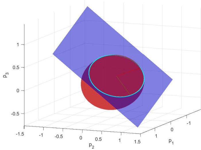
Furthermore, we need to describe the absolutely and partially constrained regions. We can see that ϕ−1​(τs,Js)\phi^{-1}\left(\tau_{s},J_{s}\right) is a hyperplane when τs\tau_{s} is held constant, and it is a hyperellipsoid when JsJ_{s} is held constant. The surface that a given abstract state maps to is the intersection of these two surfaces. We can then check the resulting intersection against the constraints given in (30). Figure 4 illustrates these inverse mappings for a 3-robot swarm. Figure 5 shows a Monte Carlo approximation of the abstract spaces and the regions within.
Refer to caption
Fig. 4: Visualization of inverse mapping of an abstract state. The plane is all swarm states such that τs=10​N⋅m\tau_{s}=10N\cdot m and the red ellipsoid is all swarm such states such that Js=1​k​g⋅m2J_{s}=1kg\cdot m^{2} for a three member swarm where m1=2​k​gm_{1}=2kg, m2=3​k​gm_{2}=3kg, and m3=3​k​gm_{3}=3kg. The cyan ellipse on the plane is the pre-image of 𝐚=[10 1]T\mathbf{a}=\left[10\ 1\right]^{T}.

III-B Parent Controller

Given the constraints found in the previous section, we can now design a controller for the parent system. This controller must have a region of attraction contained within Xp​cX_{pc}. It must also control the system while ensuring that the desired abstract state satisfies all of its constraints. Trying to control a single degree of freedom, θ\theta, using both τs\tau_{s} and JsJ_{s} independently would result in an over-actuated system. To remedy this, we specify a manifold that couples τs\tau_{s} and JsJ_{s}. We shape this manifold to exist within the interior of the absolutely constrained region of the abstract space. The distance between the manifold and the boundary of the absolutely constrained space is exploited by Theorem 2 to show that the system is both stable and satisfies given constraints.

For the parent system, we apply two different controllers: a PD controller and an Adaptive Robust Integral on the Sign of the Error (ARISE) controller based on the design proposed by Xian et al. [21] with a feed-forward adaptive term as proposed by Patre et al. [22][23]. These controllers specify a desired torque τs​d\tau_{sd}, which is treated as the input to the parent system. The desired swarm moment of inertia Js​dJ_{sd} can be determined by the position of τs​d\tau_{sd} on the constraint manifold and therefore be treated as part of the dynamics of the parent system.

The PD controller regulates the plane to a zero angle with zero velocity. Before designing the PD controller, we set Js​d=Js​d,0J_{sd}=J_{sd,0}, a constant, and linearize the damping as cc. We then linearize the dynamics about 𝐱p=0\mathbf{x}_{p}=0 and τs​d=0\tau_{sd}=0, to arrive at

𝐱˙p=[010cJ+Js​d,0]​𝐱p+[0−1J+Js​d,0]​τs​d\dot{\mathbf{x}}_{p}=\begin{bmatrix}0&1\\ 0&\frac{c}{J+J_{sd,0}}\end{bmatrix}\mathbf{x}_{p}+\begin{bmatrix}0\\ \frac{-1}{J+J_{sd,0}}\end{bmatrix}\tau_{sd} (31)

With this linearization, we can now use a linear control law:

τs​d=Kp​d​𝐱p\tau_{sd}=K_{pd}\mathbf{x}_{p} (32)

where Kp​d∈ℝ1×2K_{pd}\in\mathbb{R}^{1\times 2} is the matrix of control gains. This matrix is set so that this system is a Linear Quadratic Regulator (LQR) that minimizes the following cost function:

∫t0∞𝐱pT​Q​𝐱p​(τ)+R​τs​d2​(τ)​𝑑τ\displaystyle\int_{t_{0}}^{\infty}\mathbf{x}_{p}^{T}Q\mathbf{x}_{p}\left(\tau\right)+R\tau_{sd}^{2}\left(\tau\right)d\tau (33)

where QQ is a symmetric, positive definite matrix, RR is a positive scalar, and t0t_{0} is the initial time.

We also consider the ARISE controller, which can track trajectories bounded up to their fourth derivative in the presence of disturbances bounded up to their first derivative. We develop this controller by first rewriting the equation of motion of the parent system as

(J+Js)​θ¨+J˙s​θ˙+ff​(θ˙)+τd=−cos⁡(θ)​τs\left(J+J_{s}\right)\ddot{\theta}+\dot{J}_{s}\dot{\theta}+f_{f}\left(\dot{\theta}\right)+\tau_{d}=-\cos\left(\theta\right)\tau_{s} (34)

using the friction model

ff​(θ˙)=γ1​(tanh⁡(γ2​θ˙)−tanh⁡(γ3​θ˙))+γ4​tanh⁡(γ5​θ˙)+γ6​θ˙f_{f}\left(\dot{\theta}\right)=\gamma_{1}\left(\tanh\left(\gamma_{2}\dot{\theta}\right)-\tanh\left(\gamma_{3}\dot{\theta}\right)\right)+\gamma_{4}\tanh\left(\gamma_{5}\dot{\theta}\right)+\gamma_{6}\dot{\theta} (35)

where γi\gamma_{i} are the parameters of the friction model, and τd\tau_{d} models the Coriolis term as a bounded disturbance. The values of γi\gamma_{i} are all positive, where γ2>γ3\gamma_{2}>\gamma_{3} and γ4≤γ1\gamma_{4}\leq\gamma_{1}.

The parameters of the friction model may be estimated using system identification techniques; however, we use an adaptation law to estimate these terms. The uncertainties in the friction model and moment of inertia can be combined into a single term represented as a linear relationship between a vector of adaptive constants, λ\lambda, and a matrix that is a function of the desired state and its derivatives, YdY_{d}:

Yd​λ\displaystyle Y_{d}\lambda =[θ¨dtanh⁡(γ2​θ˙d)−tanh⁡(γ3​θ˙d)tanh⁡(γ5​θ˙d)θ˙d]T​[Jγ1γ4γ6]\displaystyle=\begin{bmatrix}\ddot{\theta}_{d}\\ \tanh\left(\gamma_{2}\dot{\theta}_{d}\right)-\tanh\left(\gamma_{3}\dot{\theta}_{d}\right)\\ \tanh\left(\gamma_{5}\dot{\theta}_{d}\right)\\ \dot{\theta}_{d}\end{bmatrix}^{T}\begin{bmatrix}J\\ \gamma_{1}\\ \gamma_{4}\\ \gamma_{6}\end{bmatrix} (36)
=J​θ¨d+ff​(θ˙d)\displaystyle=J\ddot{\theta}_{d}+f_{f}\left(\dot{\theta}_{d}\right) (37)

Note that γ1\gamma_{1}, γ4\gamma_{4}, and γ6\gamma_{6} are part of the adaptive state because fff_{f} is affine in them. The values of γ2\gamma_{2}, γ3\gamma_{3}, and γ5\gamma_{5} must be estimated; however, the ARISE controller has been proven to be robust to errors in these values [22]

Using the error terms developed in [21][22][23] given by e1=θd−θe_{1}=\theta_{d}-\theta and e2=e˙1+α1​e1e_{2}=\dot{e}_{1}+\alpha_{1}e_{1}, we apply the control law given by

τs​d​(t)=\displaystyle\tau_{sd}\left(t\right)= −sec⁡(θ⁡(t))​(Yd​λ^+(ks+1)​e2​(t)−(ks+1)​e2​(t0)+μ1​(t))\displaystyle-\sec\left(\theta\left(t\right)\right)\left(Y_{d}\hat{\lambda}+\left(k_{s}+1\right)e_{2}\left(t\right)-\left(k_{s}+1\right)e_{2}\left(t_{0}\right)+\mu_{1}\left(t\right)\right) (38)
μ˙1​(t)\displaystyle\dot{\mu}_{1}\left(t\right) =(ks+1)​α2​e2​(t)+β​s​g​n​(e2​(t))\displaystyle=\left(k_{s}+1\right)\alpha_{2}e_{2}\left(t\right)+\beta sgn\left(e_{2}\left(t\right)\right) (39)
λ^˙​(t)\displaystyle\dot{\hat{\lambda}}\left(t\right) =λ^​(t0)+Γ​Y˙dT​(τ)​e2​(τ)|τ=t0τ=t−Γ​μ2​(t)\displaystyle=\hat{\lambda}\left(t_{0}\right)+\left.\Gamma\dot{Y}_{d}^{T}\left(\tau\right)e_{2}\left(\tau\right)\right|_{\tau=t_{0}}^{\tau=t}-\Gamma\mu_{2}\left(t\right) (40)
μ˙2​(t)\displaystyle\dot{\mu}_{2}\left(t\right) =Y¨dT​(t)​e2​(t)−α2​Y˙dT​e2​(t)\displaystyle=\ddot{Y}_{d}^{T}\left(t\right)e_{2}\left(t\right)-\alpha_{2}\dot{Y}_{d}^{T}e_{2}\left(t\right) (41)

which utilizes a measurement of e1e_{1} and e2e_{2} as well as an estimate of the unknown constants, λ^\hat{\lambda}. The gains α1\alpha_{1}, α2\alpha_{2}, ksk_{s}, and β\beta as well as the adaptive gain Γ\Gamma must be sufficiently large to guarantee stability; however, these gains should not be so large that the system violates the bounds given in (64).

Note the secant term added to the controller in (38) to cancel out the cosine term in the dynamics of the parent system. This reduces the usable range of the controller to ±π2\pm\frac{\pi}{2}. However, the robots begin to slip off the plane at some |θ|<π2\left|\theta\right|<\frac{\pi}{2}; thus, this domain is larger than the constraint given in (29).

III-C Swarm Controller

The previous section derived a desired τs​d\tau_{sd} given by the two parent control laws, the PD controller (32) and the ARISE controller (38)-(41). This, along with the manifold used to calculate Js​dJ_{sd} (63) gives us a desired abstract state. This section presents controllers for achieving these abstract states for the three different swarms.

III-C1 Single Integrator Swarm

For the swarm described by (27), we use the input linearized controller simmilar to the one proposed by Belta and Kumar [11]. This control law is based on the derivative of the abstract state that is dependent on the errors in the abstract state given in (43). We first define the desired dynamics of the abstract state, where KK is a diagonal, positive definite matrix and 𝐞a\mathbf{e}_{a} is the error in the abstract state:

𝐚˙\displaystyle\dot{\mathbf{a}} =K​𝐞a+𝐚˙d\displaystyle=K\mathbf{e}_{a}+\dot{\mathbf{a}}_{d} (42)
𝐞a\displaystyle\mathbf{e}_{a} =𝐚d−𝐚=[eτeJ]\displaystyle=\mathbf{a}_{d}-\mathbf{a}=\begin{bmatrix}e_{\tau}\\ e_{J}\end{bmatrix} (43)

where 𝐚d\mathbf{a}_{d} is the desired abstract state of the swarm as specified by the parent controller.

If we take the time derivative of the abstract mapping (24) we get

𝐚˙=Φx​s​𝐱˙s\dot{\mathbf{a}}=\Phi_{xs}\dot{\mathbf{x}}_{s} (44)

where Φx​s\Phi_{xs} is the Jacobian of the mapping function ϕ\phi evaluated at the current 𝐱s\mathbf{x}_{s}. We combine (44) with (42) and the system model given in (27) to derive the control law given by

𝐮s=Φx​s†​(K​𝐞a+𝐚˙d)\mathbf{u}_{s}=\Phi_{xs}^{\dagger}\left(K\mathbf{e}_{a}+\dot{\mathbf{a}}_{d}\right) (45)

The pseudo-inverse of the Jacobian can be written in terms of a set of parameters, S0,…,S3S_{0},\dots,S_{3}, that are constant across the whole swarm:

Φx​s†=1S3​[m1​S2−m1​p1​S112​(m1​p1​S0−m1​S1)mN​S2−mN​pN​S112​(mN​pN​S0−mN​S1)]\Phi_{xs}^{\dagger}=\frac{1}{S_{3}}\begin{bmatrix}m_{1}S_{2}-m_{1}p_{1}S_{1}&\frac{1}{2}\left(m_{1}p_{1}S_{0}-m_{1}S_{1}\right)\\ \vdots&\vdots\\ m_{N}S_{2}-m_{N}p_{N}S_{1}&\frac{1}{2}\left(m_{N}p_{N}S_{0}-m_{N}S_{1}\right)\end{bmatrix} (46)

where

S0=∑i=1Nmi2,S1=∑i=1Nmi2pi,S2=∑i=1Nmi2pi2,and ​S3=∑i=1N∑j=i+1Nmi2​mj2​(pi−pj)2\begin{split}S_{0}=\displaystyle\sum_{i=1}^{N}m_{i}^{2},\ S_{1}=\displaystyle\sum_{i=1}^{N}m_{i}^{2}p_{i},\ S_{2}=\displaystyle\sum_{i=1}^{N}m_{i}^{2}p_{i}^{2},\\ \text{and }S_{3}=\displaystyle\sum_{i=1}^{N}\displaystyle\sum_{j=i+1}^{N}m_{i}^{2}m_{j}^{2}\left(p_{i}-p_{j}\right)^{2}\end{split} (47)

We can combine these sums into an auxiliary abstract state 𝐚a​u​x=[S0S1S2S3]T\mathbf{a}_{aux}=\begin{bmatrix}S_{0}&S_{1}&S_{2}&S_{3}\end{bmatrix}^{T}. Like the abstract state, this vector’s size is independent of the size of the swarm. Rather than describing how the swarm interacts with the parent system, the auxiliary abstract state describes how the swarm interacts with itself, allowing an individual swarm member to determine how it needs to move within the swarm to achieve the desired abstract state using the following control law:

us​i=1S3​[mi​S2−mi​pi​S112​(mi​pi​S0−mi​S1)]T​(K​𝐞a+𝐚˙d)u_{si}=\frac{1}{S_{3}}\begin{bmatrix}m_{i}S_{2}-m_{i}p_{i}S_{1}\\ \frac{1}{2}\left(m_{i}p_{i}S_{0}-m_{i}S_{1}\right)\end{bmatrix}^{T}\left(K\mathbf{e}_{a}+\dot{\mathbf{a}}_{d}\right) (48)

Note the singularity when S3=0S_{3}=0, which occurs when the entire swarm is concentrated at the same position on the plane. This singularity can be avoided by choosing a manifold on which the desired abstract state exists that never intersects this point. Assuming a manifold exists in the interior of the constrained space AA∪APA_{A}\cup A_{P}, another valid manifold that does not pass through the singularity can be found by translating the first one.

Since the system dynamics (23) and the parent control laws (32) and (38) are continuous and differentiable, the terms Js​dJ_{sd} from (63) and JsJ_{s} from (24) are also continuous and differentiable, and thus, necessarily uniformly continuous. Hence, the error term eJe_{J} is uniformly continuous. In addition, J˙s​d\dot{J}_{sd} is also differentiable. The control laws for the swarm, (48) and (58), are both continuous and differentiable, thus J˙s\dot{J}_{s} is also differentiable. Hence, the error term e˙J\dot{e}_{J} must be differentiable. We can now use Barbalat’s Lemma to show that if eJ→0e_{J}\rightarrow 0 as t→∞t\rightarrow\infty, then e˙J→0\dot{e}_{J}\rightarrow 0 as t→∞t\rightarrow\infty [24].

We demonstrate the stability of this controller with both parent controllers in the following theorems, which are applications of Theorems 1 and 2.

Theorem 3.

Given the error vector 𝐳=[θθ˙eτeJ]T\mathbf{z}=\begin{bmatrix}\theta&\dot{\theta}&e_{\tau}&e_{J}\end{bmatrix}^{T}, the PD control law (32) on the parent system (25) and the single integrator control law (48) on the swarm (27) asymptotically stabilizes the origin of this system if k1>0k_{1}>0, k2>J˙m​a​x2​cos⁡(θm​a​x)k_{2}>\frac{\dot{J}_{max}}{2\cos\left(\theta_{max}\right)}, K>0K>0, and 𝐳0∈S\mathbf{z}_{0}\in S, where k1k_{1} and k2k_{2} are the elements of the matrix Kp​dK_{pd} in the parent controller, KK is the controller gain for the swarm system, 𝐳0\mathbf{z}_{0} is the initial condition of the system, and SS is an estimate of the region of attraction

S={𝐳∈ℝ4|‖𝐳‖2≤θm​a​x22​η}S=\left\{\mathbf{z}\in\mathbb{R}^{4}\ |\ \left\lVert\mathbf{z}\right\rVert^{2}\leq\frac{\theta_{max}^{2}}{2\eta}\right\} (49)

where η=m​a​x​{1,J+Js​d,m​a​x2}\eta=max\left\{1,\frac{J+J_{sd,max}}{2}\right\}. The value θm​a​x\theta_{max} is a limit on the angle θ\theta such that |θ|≤θm​a​x<π2\left|\theta\right|\leq\theta_{max}<\frac{\pi}{2}.

Proof.

See Appendix A. ∎

Theorem 4.

Given the error vector 𝐳=[e1e2reτeJ]T\mathbf{z}=\begin{bmatrix}e_{1}&e_{2}&r&e_{\tau}&e_{J}\end{bmatrix}^{T} where r=e˙2+α2​e2r=\dot{e}_{2}+\alpha_{2}e_{2}, the ARISE control law (38), (39), (40), and (41) on the parent system (25) and the single integrator control law (48) on the swarm (27) asymptotically stabilize the origin of this system if α1>12\alpha_{1}>\frac{1}{2}, α2>1\alpha_{2}>1, β>ζNd+1α2​ζN˙d\beta>\zeta_{N_{d}}+\frac{1}{\alpha_{2}}\zeta_{\dot{N}_{d}}, ks>cm​a​xη3k_{s}>\frac{c_{max}}{\eta_{3}}, K>0K>0, Γ>0\Gamma>0, and ΓT=Γ\Gamma^{T}=\Gamma, where N~≤cm​a​x​‖𝐳‖\tilde{N}\leq c_{max}\left\lVert\mathbf{z}\right\rVert, and

η3=m​i​n​{2​α1−1,α2−1,1}\eta_{3}=min\left\{2\alpha_{1}-1,\alpha_{2}-1,1\right\} (50)

We define |Nd|≤ζNd\left|N_{d}\right|\leq\zeta_{N_{d}} and |N˙d|≤ζN˙d\left|\dot{N}_{d}\right|\leq\zeta_{\dot{N}_{d}} where

Nd=(J+Js)​θd˙˙˙+J˙s​θ¨d+f˙f​(θ˙d)−Y˙d​λN_{d}=(J+J_{s})\dddot{\theta_{d}}+\dot{J}_{s}\ddot{\theta}_{d}+\dot{f}_{f}\left(\dot{\theta}_{d}\right)-\dot{Y}_{d}\lambda (51)

The desired trajectory satisfies θd,θ˙d,θ¨d,θ˙˙˙d∈ℒ∞\theta_{d},\dot{\theta}_{d},\ddot{\theta}_{d},\dddot{\theta}_{d}\in\mathcal{L}_{\infty} and The origin of this system has a region of attraction

S={𝐳∈B,𝐲p∈ℝ2|‖[𝐳T𝐲pT]T‖2≤η1η2ρ2}S=\left\{\mathbf{z}\in B,\ \mathbf{y}_{p}\in\mathbb{R}^{2}\ |\ \left\lVert\begin{bmatrix}\mathbf{z}^{T}&\mathbf{y}_{p}^{T}\end{bmatrix}^{T}\right\rVert^{2}\leq\frac{\eta_{1}}{\eta_{2}}\rho^{2}\right\} (52)

where ρ=ρE−1​(2​η3−cm​a​x2​ks+2​λm​i​n)\rho=\rho_{E}^{-1}\left(2\eta_{3}-\frac{c_{max}}{2k_{s}}+2\lambda_{min}\right), λm​i​n\lambda_{min} is the smallest eigenvalue of KK, and

η1=12​min⁡{1,J+Js​d,0,λm​i​n​(Γ−1)}\eta_{1}=\frac{1}{2}\min\left\{1,J+J_{sd,0},\lambda_{min}\left(\Gamma^{-1}\right)\right\} (53)
η2=12​max⁡{2,J+Js​d,m​a​x,λm​a​x​(Γ−1)}\eta_{2}=\frac{1}{2}\max\left\{2,J+J_{sd,max},\lambda_{max}\left(\Gamma^{-1}\right)\right\} (54)
Proof.

See Appendix B. ∎

III-C2 Double Integrator Swarm

The swarm whose dynamics are given by (28) constitute a second-order system whose control input only directly effects the acceleration. For this reason, we specify second-order dynamics for the abstract state:

𝐚¨=Kp​𝐞a+Kd​𝐞˙a+𝐚¨d\ddot{\mathbf{a}}=K_{p}\mathbf{e}_{a}+K_{d}\dot{\mathbf{e}}_{a}+\ddot{\mathbf{a}}_{d} (55)

where KpK_{p} and KdK_{d} are diagonal, positive definite matrices.

We choose a control law

𝐮s=M​Φ†​(Kp​𝐞a+(Kd−Ca)​𝐞˙a−Φ˙x​s​𝐩˙+𝐚¨d)+(C+ks​d​I)​Φx​s†​𝐚˙d−ks​d​𝐩˙\mathbf{u}_{s}=M\Phi^{\dagger}\left(K_{p}\mathbf{e}_{a}+\left(K_{d}-C_{a}\right)\dot{\mathbf{e}}_{a}-\dot{\Phi}_{xs}\dot{\mathbf{p}}+\ddot{\mathbf{a}}_{d}\right)+\left(C+k_{sd}I\right)\Phi_{xs}^{\dagger}\dot{\mathbf{a}}_{d}-k_{sd}\dot{\mathbf{p}} (56)

where ks​dk_{sd} is a positive scalar that adds damping to the individual members of the swarm, II is the identity matrix, and

Ca=[Ca​11Ca​12Ca​21Ca​22]Ca​11=∑i=1Nmi​(ks​d+ci)​(S2−pi​S1)Ca​12=12​∑i=1Nmi​(ks​d+ci)​(pi​S0−S1)Ca​21=2​∑i=1Nmi​pi​(ks​d+ci)​(S2−pi​S1)Ca​22=∑i=1Nmi​pi​(ks​d+ci)​(pi​S0−S1)\begin{split}C_{a}&=\begin{bmatrix}C_{a11}&C_{a12}\\ C_{a21}&C_{a22}\end{bmatrix}\\ C_{a11}&=\sum_{i=1}^{N}m_{i}\left(k_{sd}+c_{i}\right)\left(S_{2}-p_{i}S_{1}\right)\\ C_{a12}&=\frac{1}{2}\sum_{i=1}^{N}m_{i}\left(k_{sd}+c_{i}\right)\left(p_{i}S_{0}-S_{1}\right)\\ C_{a21}&=2\sum_{i=1}^{N}m_{i}p_{i}\left(k_{sd}+c_{i}\right)\left(S_{2}-p_{i}S_{1}\right)\\ C_{a22}&=\sum_{i=1}^{N}m_{i}p_{i}\left(k_{sd}+c_{i}\right)\left(p_{i}S_{0}-S_{1}\right)\end{split} (57)

This feed-forward controller enforces the desired second-order dynamics in (55) on the abstract state, adds damping to each child system, and compensates the nonlinear effects of the damping in each child system. We build an auxiliary abstract state like we did with the single integrator system such that 𝐚a​u​x\mathbf{a}_{aux} contains all the SiS_{i} and Ca​j​kC_{ajk} terms for i=0​…​3i=0\dots 3, j=1,2j=1,2, and k=1,2k=1,2. We can now use this auxiliary abstract state along with the abstract state, desired abstract state, and the state of a member of the swarm to create a control law for that member:

us​i=1S3​[mi​S2−mi​pi​S112​(mi​pi​S0−mi​S1)]T​(mi​(Kp​𝐞a+(Kd−Ca)​𝐞˙a−Φ˙x​s​p˙i+𝐚¨d)+(ci+ks​d​i)​𝐚˙d)−ks​d​p˙iu_{si}=\frac{1}{S_{3}}\begin{bmatrix}m_{i}S_{2}-m_{i}p_{i}S_{1}\\ \frac{1}{2}\left(m_{i}p_{i}S_{0}-m_{i}S_{1}\right)\end{bmatrix}^{T}\left(m_{i}\left(K_{p}\mathbf{e}_{a}+\left(K_{d}-C_{a}\right)\dot{\mathbf{e}}_{a}-\dot{\Phi}_{xs}\dot{p}_{i}+\ddot{\mathbf{a}}_{d}\right)+\left(c_{i}+k_{sdi}\right)\dot{\mathbf{a}}_{d}\right)-k_{sd}\dot{p}_{i} (58)

Note that this control law, like the one given in (48), does not require knowledge of the other child systems’ states, only the abstract states. This system also has the same singularity point when S3=0S_{3}=0, which can be dealt with similarly. We demonstrate the stability of this controller with both parent controllers in the following theorems.

Theorem 5.

Given the error vector 𝐳=[θθ˙eτeJ]T\mathbf{z}=\begin{bmatrix}\theta&\dot{\theta}&e_{\tau}&e_{J}\end{bmatrix}^{T}, the PD control law (32) on the parent system (25), and the double integrator control law (58) on the swarm (28) asymptotically stabilizes the origin of this system if the gains for the parent controller satisfy the same conditions as Theorem 3 and if there exists some ϵ>0\epsilon>0 such that the following inequalities hold:

ϵ​kp​i+kd​i−ϵ\displaystyle\epsilon k_{pi}+k_{di}-\epsilon >0\displaystyle>0 (59)
ϵ​kp​i​kd​i−ϵ2​kp​i−ϵ4​kd​i2\displaystyle\epsilon k_{pi}k_{di}-\epsilon^{2}k_{pi}-\frac{\epsilon}{4}k_{di}^{2} >0\displaystyle>0 (60)
kp​i+1\displaystyle k_{pi}+1 >0\displaystyle>0 (61)
kp​i−ϵ2\displaystyle k_{pi}-\epsilon^{2} >0\displaystyle>0 (62)

where k1k_{1} and k2k_{2} are the elements of the matrix Kp​dK_{pd} in the parent controller, and kp​ik_{pi} and kd​ik_{di} are the iith diagonal elements of the KpK_{p} and KdK_{d} matrices, respectively.

The origin is stable with the same region of attraction as given by Theorem 3.

Proof.

See Appendix C. ∎

Theorem 6.

Given the error vector 𝐳=[e1e2reτeJ]T\mathbf{z}=\begin{bmatrix}e_{1}&e_{2}&r&e_{\tau}&e_{J}\end{bmatrix}^{T}, where r=e˙2+α2​e2r=\dot{e}_{2}+\alpha_{2}e_{2}, the ARISE control law (38), (39), (40), and (41) on the parent system (25) and the double integrator control law (58) on the swarm (28) asymptotically stabilize the origin of this system if the gains for the controller satisfy the same conditions on the ARISE controller from Theorem 4 and there exists some ϵ>0\epsilon>0 that satisfy the inequalities listed in Theorem 5.

This system has the same region of attraction as given by Theorem 4.

Proof.

See Appendix D. ∎

III-D Heterogeneous Swarm

The final swarm we consider is a heterogeneous swarm consisting of single integrator members as defined in (27) as well as double integrator members as defined in (28). To control the swarm, we simply use the control laws from (48) and (58) for single integrator members and double integrator members respectively.

We demonstrate the stability of this controller with both parent controllers in the following theorems:

Theorem 7.

Given the error vector 𝐳=[θθ˙eτeJ]T\mathbf{z}=\begin{bmatrix}\theta&\dot{\theta}&e_{\tau}&e_{J}\end{bmatrix}^{T}, the PD control law (32) on the parent system (25) and the single integrator control law (48) for single integrator members of the swarm and the double integrator control law (58) for double integrator members of the swarm asymptotically stabilizes the origin of this system if the gains on the parent controller satisfy the same conditions as stated in Theorem 3, if K>0K>0 for the single integrator controllers, and there exists some ϵ>0\epsilon>0 that satisfies the conditions given in Theorem 5.

The origin is stable with the same region of attraction as given by Theorem 3.

Proof.

See Appendix E. ∎

Theorem 8.

Given the error vector 𝐳=[e1e2reτeJ]T\mathbf{z}=\begin{bmatrix}e_{1}&e_{2}&r&e_{\tau}&e_{J}\end{bmatrix}^{T} where r=e˙2+α2​e2r=\dot{e}_{2}+\alpha_{2}e_{2}, the ARISE control law (38) (39) (40), and (41) on the parent system (25) and the single integrator control law (48) for single integrator members of the swarm and the double integrator control law (58) for double integrator members of the swarm asymptotically stabilizes the origin of this system if the gains on the parent controller satisfy the same conditions as stated in Theorem 4 and the controllers for the single and double integrator portions of the swarm satisfy the conditions given in Theorems 4 and 6 respectively.

This system has the same region of attraction as given by Theorem 4.

Proof.

See Appendix F. ∎

Note that this control law is independent of the size and composition of the swarm.

IV Simulation Results

TABLE I: Table of physical parameters of simulated system
Parameter Value Parameter Value
mm​a​xm_{max} 0.75​k​g0.75kg γ1\gamma_{1} 0.01​N0.01N
mm​i​nm_{min} 0.25​k​g0.25kg γ2\gamma_{2} 1000​s21000s^{2}
cm​a​xc_{max} 1.5​N⋅s/m1.5N\cdot s/m γ3\gamma_{3} 700​s2700s^{2}
cm​i​nc_{min} 0.5​N⋅s/m0.5N\cdot s/m γ4\gamma_{4} 0.02​N0.02N
JJ 0.5​k​g⋅m20.5kg\cdot m^{2} γ5\gamma_{5} 1000​s21000s^{2}
LL 1​m1m γ6\gamma_{6} 1​N​s˙1N\dot{s}
Refer to caption
Fig. 5: Results of mapping the vertices and edges of the 4-dimensional hypercube into the abstract space. The magenta lines are the mappings of the edges of this hypercube. The cyan line is the lower bound of the abstract domain. The dots (absolutely constrained states) and red dots (partially constrained states) are the Monte Carlo mapping used to confirm the absolutely constrained region. The green curve is the surface AcA_{c} on which the desired abstract state is constrained by (63) and (64).

We demonstrate the example controllers developed in the previous section in simulation using multiple different sized swarms. The physical parameters of the system are given in Table I. The masses of the child systems are uniformly distributed between mm​i​nm_{min} and mm​a​xm_{max}. The linear damping constants of the double integrator child systems are uniformly distributed between cm​i​nc_{min} and cm​a​xc_{max}. To compare results, we predetermine the masses and damping coefficients for the 4 child systems used in the following simulations. These values are m1=0.3552​k​gm_{1}=0.3552kg, m2=0.3532​k​gm_{2}=0.3532kg, m3=0.6762​k​gm_{3}=0.6762kg, m4=0.4596​k​gm_{4}=0.4596kg, c1=0.7290​N​s/mc_{1}=0.7290Ns/m, c2=1.4133​N​s/mc_{2}=1.4133Ns/m, c3=0.6524​N​s/mc_{3}=0.6524Ns/m, and c4=1.3258​N​s/mc_{4}=1.3258Ns/m. These swarms have a starting position of 𝐩0=[0.125​m−0.125​m0.125​m−0.125​m]T\mathbf{p}_{0}=\begin{bmatrix}0.125m&-0.125m&0.125m&-0.125m\end{bmatrix}^{T} with an initial velocity of 00.

Figure 5 shows the abstract space divided into its absolutely constrained, partially constrained, and unconstrained regions. It also shows the manifold on which our desired abstract state moves as well as the edges of the hypercube that bounds the swarm state. The chosen manifold, which lies in the interior of the absolutely constrained space, is given by

Js​d\displaystyle J_{sd} =0.0125​τs​d2+0.025\displaystyle=0.0125\tau_{sd}^{2}+0.025 (63)
|τs​d|\displaystyle\left|\tau_{sd}\right| ≤τm​a​x\displaystyle\leq\tau_{max} (64)

We now apply the various controllers designed in section III to this system in MATLAB simulation and present the results.

IV-A PD Controller

Fig. 6: Results from the simulations of PD controller. In the left column is the parent state, consisting of θ\theta (blue) and ω\omega (red). The center column shows the positions of the swarm members, and the right column shows the error in the abstract space consisting of the error in τ\tau (blue) and the error in JsJ_{s} (red). The top row is the simulation of the single integrator swarm, the center row is the simulation of the double integrator swarm, and the bottom row is the simulation of the heterogeneous swarm.

We implement the PD parent controller on the three different swarms using K=10​IK=10I, Kp=10​IK_{p}=10I, Kd=5​IK_{d}=5I, ks​d=1k_{sd}=1, and τm​a​x=5\tau_{max}=5. These are LQR gains calculated using Q=d​i​a​g​{10, 1}Q=diag\left\{10,\ 1\right\} and R=1R=1. Each swarm consists of 4 robots with the mass, damping coefficients, and initial condition listed previously. The initial angle of the plane is 0.1​r​a​d0.1rad with 00 velocity. The controller gain for the parent system is calculated to be Kp​d=[3.16233.2859]K_{pd}=\begin{bmatrix}3.1623&3.2859\end{bmatrix}. The stability of the single integrator swarm can be analyzed using Theorem 3. Gain k1k_{1} is positive, and KK is a positive definite, symmetric matrix. With θm​a​x=0.2\theta_{max}=0.2, we can calculate the region of attraction to be where ‖𝐳‖2<0.0326\left\lVert\mathbf{z}\right\rVert^{2}<0.0326. We then consider Figure 5 and determine acceptable constraints on the system to be |eJ|≤0.03\left|e_{J}\right|\leq 0.03 and |eτ|<2\left|e_{\tau}\right|<2. We find that the constrained region of attraction is ‖𝐳‖2≤0.0326\left\lVert\mathbf{z}\right\rVert^{2}\leq 0.0326, and so the initial errors 𝐳0=[0.100.02730.0288]\mathbf{z}_{0}=\begin{bmatrix}0.1&0&0.0273&0.0288\end{bmatrix} fall within this domain. We can calculate J˙m​a​x=1.9059\dot{J}_{max}=1.9059 and show that k2>J˙m​a​x2​cos⁡(θm​a​x)k_{2}>\frac{\dot{J}_{max}}{2\cos\left(\theta_{max}\right)}, and thus all the conditions for stability are satisfied. Theorem 5 can be used to show that the double integrator swarms has the same region of attraction, and thus the heterogeneous swarm does too.

Figure 6 shows the results of the simulations of the PD parent controller with all three swarm types. The left column of plots show the parent state, the center column shows the positions of all the child systems in the swarm, and the right column shows the errors in the abstract state. All simulations have the same initial conditions. The top row of plots is the results from the single integrator system, the middle row is the double integrator system, and the bottom row is the heterogeneous system. The second-order system has a clearly second-order response with some overshoot in the swarm positions due to the poles of the linearization of the double integrator system being complex. In the heterogeneous system, there is some oscillatory behavior in the swarm positions as well but not as much as in the swarm consisting of only double integrators. However, the responses of the parent system for all three swarm types are very similar.

IV-B ARISE Controller

Refer to caption
Fig. 7: Results from the simulations of ARISE controller. These plots are arranged in the same way as Figure 6.

Next, we apply the ARISE controller to parent system using the three different swarms. The ARISE controller is implemented with ks=1k_{s}=1, α1=1\alpha_{1}=1, α2=2\alpha_{2}=2, β=0.5\beta=0.5, and Γ=d​i​a​g​(10,1,1,10)\Gamma=diag\left(10,1,1,10\right), while the swarm system controllers use the same gains as the PD parent controller case. For all of these experiments, the ARISE controller attempts to track a reference trajectory θd​(t)=0.7​sin⁡(0.015​π​t)\theta_{d}\left(t\right)=0.7\sin\left(0.015\pi t\right) in the presence of a sinusoidal disturbance τd​(t)=0.1​sin⁡(0.5​t)\tau_{d}\left(t\right)=0.1\sin\left(0.5t\right). The initial state of the plane is 0.075​r​a​d0.075rad with 0 velocity. For the single integrator system, Theorem 4 can be used to determine that the constrained region of attraction is where ‖𝐳‖≤0.0394\left\lVert\mathbf{z}\right\rVert\leq 0.0394. The initial states are 𝐳p​0=[−0.075−0.0618−0.1104]T\mathbf{z}_{p0}=\begin{bmatrix}-0.075&-0.0618&-0.1104\end{bmatrix}^{T}, 𝐲p​0=[0.04340.0010.010.1]T\mathbf{y}_{p0}=\begin{bmatrix}0.0434&0.001&0.01&0.1\end{bmatrix}^{T}, and 𝐳a​0=[0.02730.0288]T\mathbf{z}_{a0}=\begin{bmatrix}0.0273&0.0288\end{bmatrix}^{T}. These initial conditions fall within this region of attraction; thus, the error system converges to 00 so long as cm​a​xc_{max} remains less than ksk_{s}. Theorem 6 can be used to show that the double integrator swarm has the same region of attraction, and thus, so does the heterogeneous swarm.

Figure 7 shows the result for the ARISE controller on all three swarms. This figure is organized in the same manner as Figure 6. The double integrator swarm, like with the PD controller, has more oscillation than the single integrator. However, unlike the PD controller, the heterogeneous system has greater oscillations. There is also more error present in the abstract state due to the sinusoidal disturbance.

Refer to caption
Fig. 8: Results from the simulations of ARISE controller with larger, heterogeneous swarms. Plots a and b show, respectively, the parent state and the swarm positions for a swarm of 10 single integrators and 10 double integrators. Plots c and d show the same for a swarm of 100 single integrators and 100 double integrators.

In addition to allowing different controllers to be used for both the parent and swarm systems, the abstraction is also independent of the size of the swarm. Figure 8 shows the results for the ARISE controller on heterogeneous swarms of 20 and 200 robots. The parent system response in these plots is very similar to the responses in the other example of the ARISE controller, the only difference being the way the swarm moves and some transients that get amplified at the beginning. Note that the larger the swarm is, the tighter its final formation due to the controller driving the swarm to the same desired moment of inertia with more total mass. Also due to the larger mass, less movement is needed within the swarm to effect the same gravity torque, resulting in less swarm motion.

V Conclusion

We propose a new approach for designing controllers for a class of systems where a swarm of subsystems acts upon a larger parent system with its own dynamics. We condense the interactions between the parent system into an abstract state of the swarm, which allows controllers for the parent system to be designed independently of the swarm. We also consider how constraints on the swarm states map to constraints in the abstract space. We then develop stability proofs with and without state constraints based on the abstract state rather than the full state of the swarm.

To validate these results, we present an example case of a passive, dynamic parent system being manipulated by a large number of child subsystems. We demonstrate the modularity of this approach by using several different controllers for the parent and swarm systems in combination. We also demonstrate with these simulations that the size and composition of the swarm do not significantly impact the performance of the controller on the parent system, and that the controllers for the child systems can used independent of the size of the swarm. This architecture can be further extended to a series or hierarchy of cascaded systems with abstractions modeling the coupling between layers.

Appendix A Proof of Theorem 3

Proof.

Let the desired abstract state lie on a continuous manifold Js​d​(τd)J_{sd}\left(\tau_{d}\right). Let |τd|≤τm​a​x\left|\tau_{d}\right|\leq\tau_{max}, and let Js​d,m​i​n≤Js​d​(τd)≤Js​d,m​a​xJ_{sd,min}\leq J_{sd}(\tau_{d})\leq J_{sd,max}, where Js​d​(0)=Js​d,m​i​nJ_{sd}\left(0\right)=J_{sd,min}.

The equation of motion (25) is linearized about the origin, including neglecting the nonlinear friction terms. This results in the following linear system:

𝐱p˙=[θ˙θ¨]=[010γ6J+Js,m​i​n]​[θθ˙]+[0−1J+Js,m​i​n]​τs​d=A​𝐱p+B​𝐮\dot{\mathbf{x}_{p}}=\begin{bmatrix}\dot{\theta}\\ \ddot{\theta}\end{bmatrix}=\begin{bmatrix}0&1\\ 0&\frac{\gamma_{6}}{J+J_{s,min}}\end{bmatrix}\begin{bmatrix}\theta\\ \dot{\theta}\end{bmatrix}+\begin{bmatrix}0\\ \frac{-1}{J+J_{s,min}}\end{bmatrix}\tau_{sd}=A\mathbf{x}_{p}+B\mathbf{u} (65)

where 𝐱p=[θθ˙]T\mathbf{x}_{p}=\begin{bmatrix}\theta&\dot{\theta}\end{bmatrix}^{T} and 𝐮=τs\mathbf{u}=\tau_{s}. We can find the controllability matrix of this system:

𝒞=[BA​B]=[0−1J+Js,m​i​n−γ6(J+Js,m​i​n)20]\mathcal{C}=\begin{bmatrix}B&AB\end{bmatrix}=\begin{bmatrix}0&\frac{-1}{J+J_{s,min}}\\ \frac{-\gamma_{6}}{\left(J+J_{s,min}\right)^{2}}&0\end{bmatrix} (66)

The controllability matrix 𝒞\mathcal{C} is full rank; thus, this system is controllable. We can then compute the control law (32) using an LQR method or pole placement, for example.

Let Vp​(𝐳p,t)V_{p}\left(\mathbf{z}_{p},t\right) be a Lyapunov candidate for this system, where 𝐳p=[θθ˙]T\mathbf{z}_{p}=\begin{bmatrix}\theta&\dot{\theta}\end{bmatrix}^{T}:

Vp​(𝐳p,t)=12​θ2+J+Js​(t)2​θ˙2V_{p}\left(\mathbf{z}_{p},t\right)=\frac{1}{2}\theta^{2}+\frac{J+J_{s}\left(t\right)}{2}\dot{\theta}^{2} (67)

This function is positive definite with η1​‖𝐳p‖2≤Vp​(𝐳p,t)≤η2​‖𝐳p‖2\eta_{1}\left\lVert\mathbf{z}_{p}\right\rVert^{2}\leq V_{p}\left(\mathbf{z}_{p},t\right)\leq\eta_{2}\left\lVert\mathbf{z}_{p}\right\rVert^{2}, where η1=min⁡{12,J+Js,m​i​n2}\eta_{1}=\min\left\{\frac{1}{2},\frac{J+J_{s,min}}{2}\right\}, η2=max⁡{12,J+Js,m​a​x2}\eta_{2}=\max\left\{\frac{1}{2},\frac{J+J_{s,max}}{2}\right\}. Thus VpV_{p} is positive definite per Theorem 4.8 in [20].

Taking the time derivative of VpV_{p} and substituting (25) and (32) yields

Vp˙=θ​θ˙+θ˙​(J+Js)​θ¨+J˙s2​θ˙2=θ​θ˙+θ˙​(−c​o​s​(θ)​(k1​θ+k2​θ˙)−J˙s​θ˙−ff​(θ˙))+J˙s2​θ˙2=−(cos⁡(θ)​k1−1)​θ​θ˙−(cos⁡(θ)​k2+J˙s2)​θ˙2−θ˙​ff​(θ˙)=−𝐳pT​[0−1cos⁡(θ)​k1cos⁡(θ)​k2+J˙s2]​𝐳p−θ˙​ff​(θ˙)\begin{split}\begin{aligned} \dot{V_{p}}&=\theta\dot{\theta}+\dot{\theta}\left(J+J_{s}\right)\ddot{\theta}+\frac{\dot{J}_{s}}{2}\dot{\theta}^{2}\\ &=\theta\dot{\theta}+\dot{\theta}\left(-cos\left(\theta\right)\left(k_{1}\theta+k_{2}\dot{\theta}\right)-\dot{J}_{s}\dot{\theta}-f_{f}\left(\dot{\theta}\right)\right)+\frac{\dot{J}_{s}}{2}\dot{\theta}^{2}\\ &=-\left(\cos\left(\theta\right)k_{1}-1\right)\theta\dot{\theta}-\left(\cos\left(\theta\right)k_{2}+\frac{\dot{J}_{s}}{2}\right)\dot{\theta}^{2}-\dot{\theta}f_{f}\left(\dot{\theta}\right)\\ &=-\mathbf{z}_{p}^{T}\begin{bmatrix}0&-1\\ \cos\left(\theta\right)k_{1}&\cos\left(\theta\right)k_{2}+\frac{\dot{J}_{s}}{2}\end{bmatrix}\mathbf{z}_{p}-\dot{\theta}f_{f}\left(\dot{\theta}\right)\end{aligned}\end{split} (68)

We assume that |θ|≤θm​a​x<π2\left|\theta\right|\leq\theta_{max}<\frac{\pi}{2}. By Lemma 1 in Appendix G, |J˙s|\left|\dot{J}_{s}\right| is bounded above; thus, define domain DJ​m​a​xD_{Jmax} on which |J˙s|<J˙m​a​x\left|\dot{J}_{s}\right|<\dot{J}_{max}. Therefore,

Vp˙≤−𝐳pT​[0−1cos⁡(θm​a​x)​k1cos⁡(θm​a​x)​k2−J˙m​a​x2]​𝐳p−θ˙​ff​(θ˙)≡−𝐳pT​M​𝐳p−θ˙​ff​(θ˙)\dot{V_{p}}\leq-\mathbf{z}_{p}^{T}\begin{bmatrix}0&-1\\ \cos\left(\theta_{max}\right)k_{1}&\cos\left(\theta_{max}\right)k_{2}-\frac{\dot{J}_{max}}{2}\end{bmatrix}\mathbf{z}_{p}\\ -\dot{\theta}f_{f}\left(\dot{\theta}\right)\equiv-\mathbf{z}_{p}^{T}M\mathbf{z}_{p}-\dot{\theta}f_{f}\left(\dot{\theta}\right) (69)

The term θ˙​ff​(θ˙)\dot{\theta}f_{f}\left(\dot{\theta}\right) is positive definite since if θ˙<0\dot{\theta}<0, then ff​(θ˙)<0f_{f}\left(\dot{\theta}\right)<0 and if θ˙>0\dot{\theta}>0, then ff​(θ˙)>0f_{f}\left(\dot{\theta}\right)>0.

The 𝐳pT​M​𝐳p\mathbf{z}_{p}^{T}M\mathbf{z}_{p} term can be bounded by

λm​i​n​‖𝐳p‖2≤𝐳pT​M​𝐳p≤λm​a​x​‖𝐳p‖2\lambda_{min}\left\lVert\mathbf{z}_{p}\right\rVert^{2}\leq\mathbf{z}_{p}^{T}M\mathbf{z}_{p}\leq\lambda_{max}\left\lVert\mathbf{z}_{p}\right\rVert^{2} (70)

where λm​i​n\lambda_{min} and λm​a​x\lambda_{max} are the minimum and maximum eigenvalues of MM, respectively. If these eigenvalues are both positive, then this term is positive definite. We find the characteristic equation of the matrix M:

λ2−(cos⁡(θm​a​x)​k2−J˙m​a​x2)​λ+cos⁡(θm​a​x)​k1=0\lambda^{2}-\left(\cos\left(\theta_{max}\right)k_{2}-\frac{\dot{J}_{max}}{2}\right)\lambda+\cos\left(\theta_{max}\right)k_{1}=0 (71)

using Routh-Hurwitz Stability Criterion [25], the following need to be true for the eigenvalues to be positive:

cos⁡(θm​a​x)​k2−J˙m​a​x2\displaystyle\cos\left(\theta_{max}\right)k_{2}-\frac{\dot{J}_{max}}{2} >0\displaystyle>0 (72)
cos⁡(θm​a​x)​k1\displaystyle\cos\left(\theta_{max}\right)k_{1} >0\displaystyle>0 (73)

Therefore, if k1>0k_{1}>0 and k2>J˙m​a​x2​cos⁡(θm​a​x)k_{2}>\frac{\dot{J}_{max}}{2\cos\left(\theta_{max}\right)}, then V˙p\dot{V}_{p} is negative definite on the domain

D={𝐳∈DJ​m​a​x||θ|≤θm​a​x}D=\left\{\mathbf{z}\in D_{Jmax}\ |\ \left|\theta\right|\leq\theta_{max}\right\} (74)

We now consider the swarm system. We propose a quadratic Lyapunov function

Va=12​𝐳aT​𝐳aV_{a}=\frac{1}{2}\mathbf{z}_{a}^{T}\mathbf{z}_{a} (75)

where

𝐳a=[eτeJ]T\mathbf{z}_{a}=\begin{bmatrix}e_{\tau}&e_{J}\end{bmatrix}^{T} (76)

This function is clearly positive definite. We then take its time derivative to arrive at

V˙a=𝐳˙aT​𝐳a=(𝐚˙d−(K​𝐳a+𝐚˙d))T​𝐳a=−𝐳aT​KT​𝐳a=V˙a′\begin{split}\dot{V}_{a}&=\dot{\mathbf{z}}_{a}^{T}\mathbf{z}_{a}\\ &=\left(\dot{\mathbf{a}}_{d}-\left(K\mathbf{z}_{a}+\dot{\mathbf{a}}_{d}\right)\right)^{T}\mathbf{z}_{a}\\ &=-\mathbf{z}_{a}^{T}K^{T}\mathbf{z}_{a}\\ &=\dot{V}_{a}^{\prime}\end{split} (77)

Therefore, if KK is positive definite, then V˙a′\dot{V}_{a}^{\prime} is negative definite on Da=ℝ2D_{a}=\mathbb{R}^{2}.

Define V=Vp+VaV=V_{p}+V_{a}. By Theorem 1, the domain on which V˙\dot{V} is negative definite is

D={𝐳∈DJ​m​a​x||θ|≤θm​a​x}D=\left\{\mathbf{z}\in D_{Jmax}\ |\ \left|\theta\right|\leq\theta_{max}\right\} (78)

The largest semilevel set that fits in this domain is

Sl={𝐳∈ℝ4|V⁡(𝐳)≤θm​a​x22}S_{l}=\left\{\mathbf{z}\in\mathbb{R}^{4}\ |\ V\left(\mathbf{z}\right)\leq\frac{\theta_{max}^{2}}{2}\right\} (79)

For simplicity, we can find the largest ball that fits into this semilevel set:

S={𝐳∈ℝ4|‖𝐳‖≤θm​a​x22​η}S=\left\{\mathbf{z}\in\mathbb{R}^{4}\ |\ \left\lVert\mathbf{z}\right\rVert\leq\frac{\theta_{max}^{2}}{2\eta}\right\} (80)

where η=m​a​x​{12,J+Js,m​a​x2}\eta=max\left\{\frac{1}{2},\frac{J+J_{s,max}}{2}\right\}. SS is a subset of the region of attraction of this system. We can use this bound on ‖𝐳‖\left\lVert\mathbf{z}\right\rVert to find J˙m​a​x\dot{J}_{max} and thus the range of k2k_{2} required to stabilize the origin of this system. ∎

Appendix B Proof of Theorem 4

Proof.

We define a new error term rr:

r=e˙2+α2​e2r=\dot{e}_{2}+\alpha_{2}e_{2} (81)

My multiplying rr by the inertia term, we arrive at

(J+Js)​r=(J+Js)​(e¨1+α1​e˙1+α2​e2)=(J+Js)​(θ¨d+α1​e˙1+α2​e2)−(J+Js)​θ¨=Yd​λ+W+c​o​s​(θ)​τs+τd\begin{split}\left(J+J_{s}\right)r&=\left(J+J_{s}\right)\left(\ddot{e}_{1}+\alpha_{1}\dot{e}_{1}+\alpha_{2}e_{2}\right)\\ &=\left(J+J_{s}\right)\left(\ddot{\theta}_{d}+\alpha_{1}\dot{e}_{1}+\alpha_{2}e_{2}\right)-\left(J+J_{s}\right)\ddot{\theta}\\ &=Y_{d}\lambda+W+cos\left(\theta\right)\tau_{s}+\tau_{d}\end{split} (82)

where

W=(J+Js)​(θ¨d+α1​e˙1+α2​e2)+J˙s​θ˙+ff​(θ˙)−Yd​λW=\left(J+J_{s}\right)\left(\ddot{\theta}_{d}+\alpha_{1}\dot{e}_{1}+\alpha_{2}e_{2}\right)+\dot{J}_{s}\dot{\theta}+f_{f}\left(\dot{\theta}\right)-Y_{d}\lambda (83)

We now rewrite the control laws (38) and (40) in terms of rr:

τs​d=−sec⁡(θ)​(Yd​λ^+μ)\tau_{sd}=-\sec\left(\theta\right)\left(Y_{d}\hat{\lambda}+\mu\right) (84)
λ^˙=Γ​Y˙dT​r\dot{\hat{\lambda}}=\Gamma\dot{Y}_{d}^{T}r (85)

where

μ⁡(t0)=0\mu\left(t_{0}\right)=0 (86)
λ^​(t0)=λ^0\hat{\lambda}\left(t_{0}\right)=\hat{\lambda}_{0} (87)
μ˙=(k​s+1)​r+β​s​g​n​(e2)\dot{\mu}=\left(ks+1\right)r+\beta sgn\left(e_{2}\right) (88)

and substitute (88), (43), and (84) into (82):

(J+Js)​r=Yd​λ+W−Yd​λ^−μ−cos⁡(θ)​eτ+τd=Yd​λ~+W−μ−cos⁡(θ)​eτ+τ˙d\begin{split}(J+J_{s})r&=Y_{d}\lambda+W-Y_{d}\hat{\lambda}-\mu-\cos\left(\theta\right)e_{\tau}+\tau_{d}\\ &=Y_{d}\tilde{\lambda}+W-\mu-\cos\left(\theta\right)e_{\tau}+\dot{\tau}_{d}\end{split} (89)

where

λ~=λ−λ^\tilde{\lambda}=\lambda-\hat{\lambda} (90)

We next take the time derivative of (89):

(J+Js)​r˙=−J˙s​r+Y˙d​λ~−Yd​λ^˙+W˙−μ˙+θ˙​sin⁡(θ)​eτ−cos⁡(θ)​e˙τ+τ˙d\left(J+J_{s}\right)\dot{r}=-\dot{J}_{s}r+\dot{Y}_{d}\tilde{\lambda}-Y_{d}\dot{\hat{\lambda}}+\dot{W}-\dot{\mu}+\dot{\theta}\sin\left(\theta\right)e_{\tau}-\cos\left(\theta\right)\dot{e}_{\tau}+\dot{\tau}_{d} (91)

and substitute (84) and (85):

(J+Js)​r˙=−J˙s​r+Y˙d​λ~−Yd​Γ​Y˙dT​r+W˙−(ks+1)​r−β​s​g​n​(e2)+θ˙​sin⁡(θ)−cos⁡(θ)​e˙τ+τ˙d=−12​J˙s​r+Y˙d​λ~+N+E−(ks+1)​r−β​s​g​n​(e2)−e2\begin{split}\left(J+J_{s}\right)\dot{r}&=-\dot{J}_{s}r+\dot{Y}_{d}\tilde{\lambda}-Y_{d}\Gamma\dot{Y}_{d}^{T}r+\dot{W}-\left(k_{s}+1\right)r-\beta sgn\left(e_{2}\right)+\dot{\theta}\sin\left(\theta\right)-\cos\left(\theta\right)\dot{e}_{\tau}+\dot{\tau}_{d}\\ &=-\frac{1}{2}\dot{J}_{s}r+\dot{Y}_{d}\tilde{\lambda}+N+E-\left(k_{s}+1\right)r-\beta sgn\left(e_{2}\right)-e_{2}\end{split} (92)

where

N=−Yd​Γ​Y˙dT​r+W˙−12​J˙s​r+e2+τdN=-Y_{d}\Gamma\dot{Y}_{d}^{T}r+\dot{W}-\frac{1}{2}\dot{J}_{s}r+e_{2}+\tau_{d} (93)
E=θ˙​sin⁡(θ)​eτ−cos⁡(θ)​e˙τE=\dot{\theta}\sin\left(\theta\right)e_{\tau}-\cos\left(\theta\right)\dot{e}_{\tau} (94)

Define

N~=N−Nd\tilde{N}=N-N_{d} (95)
E~=E−Ed\tilde{E}=E-E_{d} (96)

Then, by Lemmas 2 and 3,

|N~|≤cm​a​x​‖𝐳𝐩‖\left|\tilde{N}\right|\leq c_{max}\left\lVert\mathbf{z_{p}}\right\rVert (97)
|E~|≤ρE​(‖𝐳p‖)​‖𝐳a‖\left|\tilde{E}\right|\leq\rho_{E}\left(\left\lVert\mathbf{z}_{p}\right\rVert\right)\left\lVert\mathbf{z}_{a}\right\rVert (98)

where

𝐳p=[e1e2r]T\mathbf{z}_{p}=\begin{bmatrix}e_{1}&e_{2}&r\end{bmatrix}^{T} (99)
𝐳a=[eτeJ]T\mathbf{z}_{a}=\begin{bmatrix}e_{\tau}&e_{J}\end{bmatrix}^{T} (100)

The last auxiliary functions we need are

P⁡(t)=β​|e2​(t0)|−e2​(t0)​(Nd​(t0)+Ed​(t0))−∫t0tL⁡(σ)​𝑑σP\left(t\right)=\beta\left|e_{2}\left(t_{0}\right)\right|-e_{2}\left(t_{0}\right)\left(N_{d}\left(t_{0}\right)+E_{d}\left(t_{0}\right)\right)-\displaystyle\int_{t_{0}}^{t}L\left(\sigma\right)d\sigma (101)

where

L⁡(t)=r⁡((Nd​(t)+Ed​(t))−β​s​g​n​(e2​(t)))L\left(t\right)=r\left(\left(N_{d}\left(t\right)+E_{d}\left(t\right)\right)-\beta sgn\left(e_{2}\left(t\right)\right)\right) (102)

We now define a new vector 𝐲𝐩\mathbf{y_{p}} that contains terms that are bounded but do not necessarily converge to zero, such as error in the adaptive terms and integral terms:

𝐲𝐩=[λ~TP]T\mathbf{y_{p}}=\begin{bmatrix}\tilde{\lambda}^{T}&\sqrt{P}\end{bmatrix}^{T} (103)

and a Lyapunov candidate

Vp=e12+12​e22+12​(J+Js)​r2+P+12​λ~T​Γ−1​λ~V_{p}=e_{1}^{2}+\frac{1}{2}e_{2}^{2}+\frac{1}{2}\left(J+J_{s}\right)r^{2}+P+\frac{1}{2}\tilde{\lambda}^{T}\Gamma^{-1}\tilde{\lambda} (104)

By Lemma 4, ∫t0tL⁡(σ)​𝑑σ≤β​|e2​(t0)|−ed​(t0)​(Nd​(t0)+Ed​(t0))\int_{t_{0}}^{t}L\left(\sigma\right)d\sigma\leq\beta\left|e_{2}\left(t_{0}\right)\right|-e_{d}\left(t_{0}\right)\left(N_{d}\left(t_{0}\right)+E_{d}\left(t_{0}\right)\right). Thus we can show that P≥0P\geq 0, and so P∈ℝ\sqrt{P}\in\mathbb{R} and

η1​‖[𝐳pT𝐲pT]T‖≤Vp≤η2​‖[𝐳pT𝐲pT]T‖\eta_{1}\left\lVert\begin{bmatrix}\mathbf{z}_{p}^{T}&\mathbf{y}_{p}^{T}\end{bmatrix}^{T}\right\rVert\leq V_{p}\leq\eta_{2}\left\lVert\begin{bmatrix}\mathbf{z}_{p}^{T}&\mathbf{y}_{p}^{T}\end{bmatrix}^{T}\right\rVert (105)

where

η1=12​min⁡{1,J+Js,m​i​n,λm​i​n​(Γ−1)}\eta_{1}=\frac{1}{2}\min\left\{1,J+J_{s,min},\lambda_{min}\left(\Gamma^{-1}\right)\right\} (106)
η2=12​max⁡{2,J+Js,m​a​x,λm​a​x​(Γ−1)}\eta_{2}=\frac{1}{2}\max\left\{2,J+J_{s,max},\lambda_{max}\left(\Gamma^{-1}\right)\right\} (107)

We can prove this by writing Vp=[𝐳pT𝐲pT]​Q​[𝐳pT𝐲pT]TV_{p}=\begin{bmatrix}\mathbf{z}_{p}^{T}&\mathbf{y}_{p}^{T}\end{bmatrix}Q\begin{bmatrix}\mathbf{z}_{p}^{T}&\mathbf{y}_{p}^{T}\end{bmatrix}^{T}, where QQ is a block diagonal matrix in which each of the terms in (104) contributes a block. All of the blocks are 1-dimensional except for Γ\Gamma. η1\eta_{1} and η2\eta_{2} are the minimum and maximum eigenvalues of QQ, which are positive if Γ\Gamma is positive definite; thus our Lyapunov candidate is positive definite. Note also that Lemma 4 gives the lower bound on β\beta.

We then take the time derivative and substitute the control laws (38) and (40) to show that V˙p\dot{V}_{p} is negative semi-definite:

Vp˙=2​e1​e˙1+e2​e˙2+(J+Js)​r˙​r+12​J˙s​r2+P˙−λ~​Γ−1​λ^˙=2​e1​(e2−α1​e1)+e2​(r−α2​e2)+−12​J˙s​r2+Y˙d​λ~​r+(N+E)​r−(ks+1)​r2−β​s​g​n​(e2)​r−e2​r+12​J˙s​r2−L−λ~T​Γ−1​Γ​Y˙dT​r=−2​α1​e12−α2​e22−(ks+1)​r2+2​e1​e2+(N~+E~)​r+(Nd+Ed)​r−β​s​g​n​(e2)​r−r⁡(Nd+Ed−β​s​g​n​(e2))=−2​α1​e12−α2​e22−(ks+1)​r2+2​e1​e2+(N~+E~)​r≤−(2​α1−1)​e12−(α2−1)​e22−(ks+1)​r2+(N~+E~)​r≤−η3​‖𝐳p‖2−(ks​r2−cm​a​x​‖𝐳p‖​|r|)+ρE​(‖𝐳p‖)​‖𝐳a‖​‖𝐳p‖\begin{split}\dot{V_{p}}&=2e_{1}\dot{e}_{1}+e_{2}\dot{e}_{2}+\left(J+J_{s}\right)\dot{r}r+\frac{1}{2}\dot{J}_{s}r^{2}+\dot{P}-\tilde{\lambda}\Gamma^{-1}\dot{\hat{\lambda}}\\ &=2e_{1}\left(e_{2}-\alpha_{1}e_{1}\right)+e_{2}\left(r-\alpha_{2}e_{2}\right)+-\frac{1}{2}\dot{J}_{s}r^{2}+\dot{Y}_{d}\tilde{\lambda}r+\left(N+E\right)r-\left(k_{s}+1\right)r^{2}\\ &\phantom{=}-\beta sgn\left(e_{2}\right)r-e_{2}r+\frac{1}{2}\dot{J}_{s}r^{2}-L-\tilde{\lambda}^{T}\Gamma^{-1}\Gamma\dot{Y}_{d}^{T}r\\ &=-2\alpha_{1}e_{1}^{2}-\alpha_{2}e_{2}^{2}-\left(k_{s}+1\right)r^{2}+2e_{1}e_{2}+\left(\tilde{N}+\tilde{E}\right)r+\left(N_{d}+E_{d}\right)r-\beta sgn\left(e_{2}\right)r\\ &\phantom{=}-r\left(N_{d}+E_{d}-\beta sgn\left(e_{2}\right)\right)\\ &=-2\alpha_{1}e_{1}^{2}-\alpha_{2}e_{2}^{2}-\left(k_{s}+1\right)r^{2}+2e_{1}e_{2}+\left(\tilde{N}+\tilde{E}\right)r\\ &\leq-\left(2\alpha_{1}-1\right)e_{1}^{2}-\left(\alpha_{2}-1\right)e_{2}^{2}-\left(k_{s}+1\right)r^{2}+\left(\tilde{N}+\tilde{E}\right)r\\ &\leq-\eta_{3}\left\lVert\mathbf{z}_{p}\right\rVert^{2}-\left(k_{s}r^{2}-c_{max}\left\lVert\mathbf{z}_{p}\right\rVert\left|r\right|\right)+\rho_{E}\left(\left\lVert\mathbf{z}_{p}\right\rVert\right)\left\lVert\mathbf{z}_{a}\right\rVert\left\lVert\mathbf{z}_{p}\right\rVert\end{split} (108)

where η3=m​i​n​{2​α1−1,α2−1,1}\eta_{3}=min\left\{2\alpha_{1}-1,\alpha_{2}-1,1\right\}. Thus α1>12\alpha_{1}>\frac{1}{2} and α2>1\alpha_{2}>1 make η3\eta_{3} positive and thus make V˙p′\dot{V}_{p}^{\prime} negative definite. We break this into its uncoupled and coupled terms per Theorem 1:

Vp′\displaystyle{V}_{p}^{\prime} =−η3​‖𝐳p‖2−(ks​r2−cm​a​x​‖𝐳p‖​|r|)\displaystyle=-\eta_{3}\left\lVert\mathbf{z}_{p}\right\rVert^{2}-\left(k_{s}r^{2}-c_{max}\left\lVert\mathbf{z}_{p}\right\rVert\left|r\right|\right) (109)
V˙c​p\displaystyle\dot{V}_{cp} =ρE​(‖𝐳p‖)​‖𝐳a‖​‖𝐳p‖\displaystyle=\rho_{E}\left(\left\lVert\mathbf{z}_{p}\right\rVert\right)\left\lVert\mathbf{z}_{a}\right\rVert\left\lVert\mathbf{z}_{p}\right\rVert (110)

We complete the square on (108) to get

V˙p′≤−η3​‖𝐳p‖2−((ks​|r|−cm​a​x​‖𝐳p‖2​ks)2−cm​a​x2​‖𝐳p‖24​ks)≤−η3​‖𝐳p‖2+cm​a​x2​‖𝐳p‖24​ks−(ks​|r|−cm​a​x​‖𝐳p‖2​ks)2≤−(η3−cm​a​x4​ks)​‖𝐳p‖2\begin{split}\begin{aligned} \dot{V}_{p}^{\prime}&\leq-\eta_{3}\left\lVert\mathbf{z}_{p}\right\rVert^{2}-\left(\left(\sqrt{k_{s}}\left|r\right|-\frac{c_{max}\left\lVert\mathbf{z}_{p}\right\rVert}{2\sqrt{k_{s}}}\right)^{2}-\frac{c_{max}^{2}\left\lVert\mathbf{z}_{p}\right\rVert^{2}}{4k_{s}}\right)\\ &\leq-\eta_{3}\left\lVert\mathbf{z}_{p}\right\rVert^{2}+\frac{c_{max}^{2}\left\lVert\mathbf{z}_{p}\right\rVert^{2}}{4k_{s}}-\left(\sqrt{k_{s}}\left|r\right|-\frac{c_{max}\left\lVert\mathbf{z}_{p}\right\rVert}{2\sqrt{k_{s}}}\right)^{2}\\ &\leq-\left(\eta_{3}-\frac{c_{max}}{4k_{s}}\right)\left\lVert\mathbf{z}_{p}\right\rVert^{2}\end{aligned}\end{split} (111)

which is negative definite if ks>cm​a​x4​η3k_{s}>\frac{c_{max}}{4\eta_{3}} on Dp=ℝ3D_{p}=\mathbb{R}^{3}.

We use the same Lyapunov function for the swarm as Theorem 3:

Va=12​𝐳aT​𝐳aV_{a}=\frac{1}{2}\mathbf{z}_{a}^{T}\mathbf{z}_{a} (112)

With these two Lyapunov functions, VpV_{p} and VaV_{a}, we can say that by Theorem 1, 𝐳p\mathbf{z}_{p} and 𝐳a\mathbf{z}_{a} asymptotically converge to the origin and 𝐲p\mathbf{y}_{p} is bounded, so long as

(η3−cm​a​x4​ks)​‖𝐳p‖2+𝐳aT​KT​𝐳a>ρE​(‖𝐳p‖)​‖𝐳p‖​‖𝐳a‖\left(\eta_{3}-\frac{c_{max}}{4k_{s}}\right)\left\lVert\mathbf{z}_{p}\right\rVert^{2}+\mathbf{z}_{a}^{T}K^{T}\mathbf{z}_{a}>\rho_{E}\left(\left\lVert\mathbf{z}_{p}\right\rVert\right)\left\lVert\mathbf{z}_{p}\right\rVert\left\lVert\mathbf{z}_{a}\right\rVert (113)

Let 𝐳′=[𝐳pT𝐳aT]T\mathbf{z}^{\prime}=\begin{bmatrix}\mathbf{z}_{p}^{T}&\mathbf{z}_{a}^{T}\end{bmatrix}^{T}. We specify a domain DD on which (113) is satisfied:

D={𝐳∈Dp×Da∣(η3−cm​a​x4​ks)​‖𝐳p‖2+𝐳aT​KT​𝐳a>ρE​(‖𝐳p‖)​‖𝐳p‖​‖𝐳a‖}D=\left\{\mathbf{z}\in D_{p}\times D_{a}\mid\left(\eta_{3}-\frac{c_{max}}{4k_{s}}\right)\left\lVert\mathbf{z}_{p}\right\rVert^{2}+\mathbf{z}_{a}^{T}K^{T}\mathbf{z}_{a}>\rho_{E}\left(\left\lVert\mathbf{z}_{p}\right\rVert\right)\left\lVert\mathbf{z}_{p}\right\rVert\left\lVert\mathbf{z}_{a}\right\rVert\right\} (114)

By Theorem 1, we can find a region of attraction SS in which the initial state must be for the system to converge.

We can see that

(η3−cm​a​x4​ks)​‖𝐳p‖2+𝐳aT​KT​𝐳a≥(η3−cm​a​x4​ks)​‖𝐳‖2+λm​i​n​‖𝐳‖\left(\eta_{3}-\frac{c_{max}}{4k_{s}}\right)\left\lVert\mathbf{z}_{p}\right\rVert^{2}+\mathbf{z}_{a}^{T}K^{T}\mathbf{z}_{a}\geq\left(\eta_{3}-\frac{c_{max}}{4k_{s}}\right)\left\lVert\mathbf{z}\right\rVert^{2}+\lambda_{min}\left\lVert\mathbf{z}\right\rVert (115)

and

ρE​(‖𝐳p‖)​‖𝐳p‖​‖𝐳a‖≤12​ρE​(‖𝐳p‖)​‖𝐳‖2\rho_{E}\left(\left\lVert\mathbf{z}_{p}\right\rVert\right)\left\lVert\mathbf{z}_{p}\right\rVert\left\lVert\mathbf{z}_{a}\right\rVert\leq\frac{1}{2}\rho_{E}\left(\left\lVert\mathbf{z}_{p}\right\rVert\right)\left\lVert\mathbf{z}\right\rVert^{2} (116)

where λm​i​n\lambda_{min} in the minimum eigenvalue of KK. Thus we can find the largest ball BB within the domain DD:

B={𝐳∈D|‖𝐳‖≤ρE−1​(2​η3−cm​a​x2​ks+2​λm​i​n)}B=\left\{\mathbf{z}\in D\ |\ \left\lVert\mathbf{z}\right\rVert\leq\rho_{E}^{-1}\left(2\eta_{3}-\frac{c_{max}}{2k_{s}}+2\lambda_{min}\right)\right\} (117)

The boundary of this ball is much easier to compute than the boundary of DD; thus, we can use its boundary to find a semilevel set SS that is contained within the region of attraction of this system:

Sl={𝐳∈B,𝐲p∈ℝ2|Vp(𝐳,𝐲p)+Va(𝐳)≤η1ρ2}S_{l}=\left\{\mathbf{z}\in B,\ \mathbf{y}_{p}\in\mathbb{R}^{2}\ |\ V_{p}\left(\mathbf{z},\mathbf{y}_{p}\right)+V_{a}\left(\mathbf{z}\right)\leq\eta_{1}\rho^{2}\right\} (118)

where ρ=ρE−1​(2​η3−cm​a​x2​ks+2​λm​i​n)\rho=\rho_{E}^{-1}\left(2\eta_{3}-\frac{c_{max}}{2k_{s}}+2\lambda_{min}\right).

Like in the proof for Theorem 3, we can find the largest ball within this set to simplify our calculations later:

S={𝐳∈B,𝐲p∈ℝ2|‖[𝐳T𝐲pT]T‖≤η1η2ρ2}S=\left\{\mathbf{z}\in B,\ \mathbf{y}_{p}\in\mathbb{R}^{2}\ |\ \left\lVert\begin{bmatrix}\mathbf{z}^{T}&\mathbf{y}_{p}^{T}\end{bmatrix}^{T}\right\rVert\leq\frac{\eta_{1}}{\eta_{2}}\rho^{2}\right\} (119)

Thus, SS is a subset of the region of attraction of this system. ∎

Appendix C Proof of Theorem 5

Proof.

First we propose a Lyapunov candidate for the swarm system:

Va=12​𝐳aT​[Kpϵ​Iϵ​II]​𝐳a≡12​𝐳aT​M1​𝐳aV_{a}=\frac{1}{2}\mathbf{z}_{a}^{T}\begin{bmatrix}K_{p}&\epsilon I\\ \epsilon I&I\end{bmatrix}\mathbf{z}_{a}\equiv\frac{1}{2}\mathbf{z}_{a}^{T}M_{1}\mathbf{z}_{a} (120)

where 𝐳a=[𝐞aT𝐞˙aT]T\mathbf{z}_{a}=\begin{bmatrix}\mathbf{e}_{a}^{T}&\dot{\mathbf{e}}_{a}^{T}\end{bmatrix}^{T}.

We can say that λm​i​n​‖𝐳a‖2≤Va≤λm​a​x​‖𝐳a‖2\lambda_{min}\left\lVert\mathbf{z}_{a}\right\rVert^{2}\leq V_{a}\leq\lambda_{max}\left\lVert\mathbf{z}_{a}\right\rVert^{2} where λm​i​n\lambda_{min} and λm​a​x\lambda_{max} are the minimum and maximum eigenvalues of M1M_{1}, respectively. Therefore, this function is positive definite if all the eigenvalues of M1M_{1} are positive. The eigenvalues of M1M_{1} can be found from

det(M1−λ​I)=det((Kp−λ​I)​(1−λ)​I−ϵ2​I)=det(λ2​I−(Kp+I)​λ+Kp−ϵ2​I)=(λ2−(kp​1+1)​λ+kp​1−ϵ2)​(λ2−(kp​2+1)​λ+kp​2−ϵ2)\begin{split}\det\left(M_{1}-\lambda I\right)&=\det\left(\left(K_{p}-\lambda I\right)\left(1-\lambda\right)I-\epsilon^{2}I\right)\\ &=\det\left(\lambda^{2}I-\left(K_{p}+I\right)\lambda+K_{p}-\epsilon^{2}I\right)\\ &\begin{aligned} =&\left(\lambda^{2}-\left(k_{p1}+1\right)\lambda+k_{p1}-\epsilon^{2}\right)\left(\lambda^{2}-\left(k_{p2}+1\right)\lambda+k_{p2}-\epsilon^{2}\right)\end{aligned}\end{split} (121)

where kp​ik_{pi} is the iith diagonal element of KpK_{p}. From here we can see that to have positive eigenvalues, the following must be true:

kp​i−ϵ2>0k_{pi}-\epsilon^{2}>0 (122)

for i={1, 2}i=\left\{1,\ 2\right\}.

Next we consider the time derivative of the Lyapunov candidate:

V˙a=𝐳aT​M1​𝐳˙a=𝐞aT​Kp​𝐞˙a+ϵ​𝐞aT​𝐞¨a+ϵ​𝐞˙aT​𝐞˙a+𝐞˙aT​𝐞¨a\begin{split}\dot{V}_{a}&=\mathbf{z}_{a}^{T}M_{1}\dot{\mathbf{z}}_{a}\\ &=\mathbf{e}_{a}^{T}K_{p}\dot{\mathbf{e}}_{a}+\epsilon\mathbf{e}_{a}^{T}\ddot{\mathbf{e}}_{a}+\epsilon\dot{\mathbf{e}}_{a}^{T}\dot{\mathbf{e}}_{a}+\dot{\mathbf{e}}_{a}^{T}\ddot{\mathbf{e}}_{a}\end{split} (123)

We then substitute the swarm equation of motion (28) and control law (55):

V˙a=𝐞aT​Kp​𝐞˙a+ϵ​𝐞˙aT​𝐞˙a+(ϵ​𝐞aT+𝐞˙aT)​(𝐚¨d−Φ˙​𝐩˙CLOSE−Φ​M​(M−1​Φ†​(Kp​𝐞a+(Kd−Ca)​𝐞˙a−Φ˙​𝐩˙+𝐚¨d)CLOSEOPENOPEN(ks​d​I+C)​Φ†​𝐚˙d−(ks​d​I+C)​𝐩˙))\begin{split}\dot{V}_{a}&=\mathbf{e}_{a}^{T}K_{p}\dot{\mathbf{e}}_{a}+\epsilon\dot{\mathbf{e}}_{a}^{T}\dot{\mathbf{e}}_{a}+\left(\epsilon\mathbf{e}_{a}^{T}+\dot{\mathbf{e}}_{a}^{T}\right)\left(\ddot{\mathbf{a}}_{d}-\dot{\Phi}\dot{\mathbf{p}}\right.\\ &\phantom{=}-\Phi M\left(M^{-1}\Phi^{\dagger}\left(K_{p}\mathbf{e}_{a}+\left(K_{d}-C_{a}\right)\dot{\mathbf{e}}_{a}-\dot{\Phi}\dot{\mathbf{p}}+\ddot{\mathbf{a}}_{d}\right)\right.\\ &\phantom{=}\left.\left.\left(k_{sd}I+C\right)\Phi^{\dagger}\dot{\mathbf{a}}_{d}-\left(k_{sd}I+C\right)\dot{\mathbf{p}}\right)\right)\end{split} (124)

This expression can then be simplified to

V˙a=−ϵ​𝐞aT​Kp​𝐞a−ϵ​𝐞aT​Kd​𝐞˙a−𝐞˙aT​(Kd−ϵ​I)​𝐞˙a=𝐳aT​[−ϵ​Kp−ϵ2​Kd−ϵ2​Kd−Kd+ϵ​I]​𝐳a=𝐳aT​M2​𝐳a\begin{split}\dot{V}_{a}&=-\epsilon\mathbf{e}_{a}^{T}K_{p}\mathbf{e}_{a}-\epsilon\mathbf{e}_{a}^{T}K_{d}\dot{\mathbf{e}}_{a}-\dot{\mathbf{e}}_{a}^{T}\left(K_{d}-\epsilon I\right)\dot{\mathbf{e}}_{a}\\ &=\mathbf{z}_{a}^{T}\begin{bmatrix}-\epsilon K_{p}&-\frac{\epsilon}{2}K_{d}\\ -\frac{\epsilon}{2}K_{d}&-K_{d}+\epsilon I\end{bmatrix}\mathbf{z}_{a}\\ &=\mathbf{z}_{a}^{T}M_{2}\mathbf{z}_{a}\end{split} (125)

Therefore, for Va˙\dot{V_{a}} to be negative, the eigenvalues of M2M_{2} must be negative. We can find the eigenvalues of M2M_{2} by finding det(M2−λ​I)=0\det\left(M_{2}-\lambda I\right)=0:

0=det((ϵ​Kp+λ​I)​(Kd+(λ−ϵ)​I)−ϵ24​Kd2)=det(λ2​I+(ϵ​Kp+Kd−ϵ​I)​λ+ϵ​Kp​Kd−ϵ2​Kp−ϵ24​Kd2)=(λ2+(ϵ​kp​1+kd​1−ϵ)​λ+ϵ​kp​1​kd​1−ϵ2​kp​12−ϵ24​kd​12)(λ2+(ϵ​kp​2+kd​2−ϵ)​λ+ϵ​kp​2​kd​2−ϵ2​kp​22−ϵ24​kd​22)\begin{split}0&=\det\left(\left(\epsilon K_{p}+\lambda I\right)\left(K_{d}+\left(\lambda-\epsilon\right)I\right)-\frac{\epsilon^{2}}{4}K_{d}^{2}\right)\\ &\begin{aligned} =&\det\left(\lambda^{2}I+\left(\epsilon K_{p}+K_{d}-\epsilon I\right)\lambda+\epsilon K_{p}K_{d}-\epsilon^{2}K_{p}-\frac{\epsilon^{2}}{4}K_{d}^{2}\right)\end{aligned}\\ &\begin{aligned} =&\left(\lambda^{2}+\left(\epsilon k_{p1}+k_{d1}-\epsilon\right)\lambda+\epsilon k_{p1}k_{d1}-\epsilon^{2}k_{p1}^{2}-\frac{\epsilon^{2}}{4}k_{d1}^{2}\right)\\ &\left(\lambda^{2}+\left(\epsilon k_{p2}+k_{d2}-\epsilon\right)\lambda+\epsilon k_{p2}k_{d2}-\epsilon^{2}k_{p2}^{2}-\frac{\epsilon^{2}}{4}k_{d2}^{2}\right)\end{aligned}\end{split} (126)

where kd​ik_{di} is the iith diagonal element of KdK_{d}. From here, we can see that to get negative real parts for the eigenvalues, the following conditions must be met:

ϵ​kp​i+kd​i−ϵ\displaystyle\epsilon k_{pi}+k_{di}-\epsilon >0\displaystyle>0 (127)
ϵ​kp​i​kd​i−ϵ2​kp​i2−ϵ24​kd​i2\displaystyle\epsilon k_{pi}k_{di}-\epsilon^{2}k_{pi}^{2}-\frac{\epsilon^{2}}{4}k_{di}^{2} >0\displaystyle>0 (128)

for i={1, 2}i=\left\{1,\ 2\right\}.

For this Lyapunov candidate, V˙a≤V˙a′=λm​a​x​(M2)​‖𝐳a‖\dot{V}_{a}\leq\dot{V}_{a}^{\prime}=\lambda_{max}(M_{2})\left\lVert\mathbf{z}_{a}\right\rVert, and there are no coupling terms.

We can use the Lyapunov candidate VpV_{p} from the proof of Theorem 3. If k1>0k_{1}>0, k2>J˙m​a​xcos⁡(θm​a​x)k_{2}>\frac{\dot{J}_{max}}{\cos\left(\theta_{max}\right)}, and there exists some ϵ\epsilon that satisfies (59), (60), (61), and (62), then by Theorem 1, there exists a Lyapunov candidate for the combined system V=Vp+VaV=V_{p}+V_{a} that proves the origin of the combined system is locally asymptotically stable on a region of attraction

S={𝐳∈ℝ6|V⁡(𝐳)≤θm​a​x22}S=\left\{\mathbf{z}\in\mathbb{R}^{6}\ |\ V\left(\mathbf{z}\right)\leq\frac{\theta_{max}^{2}}{2}\right\} (129)

where 𝐳=[𝐳𝐩T𝐳aT]T\mathbf{z}=\begin{bmatrix}\mathbf{z_{p}}^{T}&\mathbf{z}_{a}^{T}\end{bmatrix}^{T}. ∎

Appendix D Proof of Theorem 6

Proof.

We can use the same Lyapunove candidate for the swarm system from the proof for Theorem 5:

Va=12​𝐳aT​[Kpϵ​Iϵ​II]​𝐳a=𝐳aT​M1​𝐳aV_{a}=\frac{1}{2}\mathbf{z}_{a}^{T}\begin{bmatrix}K_{p}&\epsilon I\\ \epsilon I&I\end{bmatrix}\mathbf{z}_{a}=\mathbf{z}_{a}^{T}M_{1}\mathbf{z}_{a} (130)

We can show that this is positive definite and its derivative is negative definite if

ϵ​kp​i+kd​i−ϵ\displaystyle\epsilon k_{pi}+k_{di}-\epsilon >0\displaystyle>0 (131)
ϵ​kp​i​kd​i−ϵ2​kp​i−ϵ4​kd​i2\displaystyle\epsilon k_{pi}k_{di}-\epsilon^{2}k_{pi}-\frac{\epsilon}{4}k_{di}^{2} >0\displaystyle>0 (132)
kp​i+1\displaystyle k_{pi}+1 >0\displaystyle>0 (133)
kp​i−ϵ2\displaystyle k_{pi}-\epsilon^{2} >0\displaystyle>0 (134)

We can use the Lyapunov candidate VpV_{p} from the proof to Theorem 4 for the parent system. If α1>12\alpha_{1}>\frac{1}{2}, α2>1\alpha_{2}>1, β>ζNd+1α2​ζd​o​t​Nd\beta>\zeta_{N_{d}}+\frac{1}{\alpha_{2}}\zeta_{\\ dot{N}_{d}}, ks>cm​a​x4​η3k_{s}>\frac{c_{max}}{4\eta_{3}}, Γ>0\Gamma>0, ΓT=Γ\Gamma^{T}=\Gamma, and there exists some ϵ\epsilon that satisfies (59), (60), (61), and (62), then by Theorem 1, there exists a Lyapunov candidate for the combined system V=Vp+VaV=V_{p}+V_{a} that proves the origin of the combined system is locally stable where 𝐳p,𝐳a→0\mathbf{z}_{p},\mathbf{z}_{a}\to 0 while 𝐲p\mathbf{y}_{p} remains bounded on a region of attraction

S={𝐳∈ℝ9|‖𝐳‖2≤η1η2​ρ2}S=\left\{\mathbf{z}\in\mathbb{R}^{9}\ |\ \left\lVert\mathbf{z}\right\rVert^{2}\leq\frac{\eta_{1}}{\eta_{2}}\rho^{2}\right\} (135)

where 𝐳=[𝐳pT𝐲pT𝐳aT]T\mathbf{z}=\begin{bmatrix}\mathbf{z}_{p}^{T}&\mathbf{y}_{p}^{T}&\mathbf{z}_{a}^{T}\end{bmatrix}^{T} and η1\eta_{1}, η2\eta_{2}, and ρ\rho are defined in Theorem 4. ∎

Appendix E Proof of Theorem 7

Proof.

We break the swarm into two parts, the single integrator swarm with a state za​sz_{as}, and the double integrator swarm za​dz_{ad}. We choose the Lyapunov candidate Va=Va​s+Va​dV_{a}=V_{as}+V_{ad}, where Va​s=12​𝐳a​sT​𝐳a​sV_{as}=\frac{1}{2}\mathbf{z}_{as}^{T}\mathbf{z}_{as} from the proof of Theorem 3. Va​d=12​𝐳a​dT​M1​𝐳a​dV_{ad}=\frac{1}{2}\mathbf{z}_{ad}^{T}M_{1}\mathbf{z}_{ad} from the proof of Theorem 5. We can use the same proofs of these theorems to show that VaV_{a} is positive definite under the given conditions.

We can show that V˙a\dot{V}_{a} is negative definite because V˙a=V˙a​s+V˙s​d\dot{V}_{a}=\dot{V}_{as}+\dot{V}_{sd}, and we can show the these two terms are negative definite as in the proofs of Theorems 3 and 5. Also note that neither function has a coupling term, so V˙a​c=0\dot{V}_{ac}=0 for the heterogeneous swarm as well.

We can use the Lyapunov candidate VpV_{p} from the proof of Theorem 3. If k1>0k_{1}>0, k2>J˙m​a​xcos⁡(θm​a​x)k_{2}>\frac{\dot{J}_{max}}{\cos\left(\theta_{max}\right)}, and there exists some ϵ\epsilon that satisfies (59), (60), (61), and (62), then by Theorem 1, there exists a Lyapunov candidate for the combined system V=Vp+VaV=V_{p}+V_{a} that proves the origin of the combined system is locally asymptotically stable on a region of attraction

S={𝐳∈ℝ6|V⁡(𝐳)≤θm​a​x22}S=\left\{\mathbf{z}\in\mathbb{R}^{6}\ |\ V\left(\mathbf{z}\right)\leq\frac{\theta_{max}^{2}}{2}\right\} (136)

where 𝐳=[𝐳𝐩T𝐳aT]T\mathbf{z}=\begin{bmatrix}\mathbf{z_{p}}^{T}&\mathbf{z}_{a}^{T}\end{bmatrix}^{T}. ∎

Appendix F Proof of Theorem 8

Proof.

We can use the same Lyapunov candidate VaV_{a} from the proof of Theorem 7 and the Lyapunov candidate VpV_{p} from the proof of Theorem 4. If α1>12\alpha_{1}>\frac{1}{2}, α2>1\alpha_{2}>1, β>ζNd+1α2​ζN˙d\beta>\zeta_{N_{d}}+\frac{1}{\alpha_{2}}\zeta_{\dot{N}_{d}}, ks>cm​a​x4​η3k_{s}>\frac{c_{max}}{4\eta_{3}}, Γ>0\Gamma>0, ΓT=Γ\Gamma^{T}=\Gamma, and there exists some ϵ\epsilon that satisfies (59), (60), (61), and (62), then by Theorem 1, there exists a Lyapunov candidate for the combined system V=Vp+VaV=V_{p}+V_{a} that proves the origin of the combined system is locally stable, where 𝐳p,𝐳a→0\mathbf{z}_{p},\mathbf{z}_{a}\to 0 while 𝐲p\mathbf{y}_{p} remains bounded on a region of attraction

S={𝐳∈ℝ9|‖𝐳‖2≤η1η2​ρ2}S=\left\{\mathbf{z}\in\mathbb{R}^{9}\ |\ \left\lVert\mathbf{z}\right\rVert^{2}\leq\frac{\eta_{1}}{\eta_{2}}\rho^{2}\right\} (137)

where 𝐳=[𝐳pT𝐲pT𝐳aT]T\mathbf{z}=\begin{bmatrix}\mathbf{z}_{p}^{T}&\mathbf{y}_{p}^{T}&\mathbf{z}_{a}^{T}\end{bmatrix}^{T} and η1\eta_{1}, η2\eta_{2}, and ρ\rho are defined in the proof of Theorem 4. ∎

Appendix G Supporting Lemmas

Lemma 1.

Given some J˙m​a​x>0\dot{J}_{max}>0, the constraints on Js​dJ_{sd} given in theorem 3, the PD control law given in (32), and the swarm control law given in (42), we can find a bounded domain DJ​m​a​x⊂DD_{Jmax}\subset D where |J˙s|≤J˙m​a​x\left|\dot{J}_{s}\right|\leq\dot{J}_{max} for all 𝐳∈DJ​m​a​x\mathbf{z}\in D_{Jmax} if ∂Js​d∂τs​d\frac{\partial J_{sd}}{\partial\tau_{sd}} is finite on DD.

Proof.

We start with the definition of eJe_{J} from (43), substitute (63), and solve for JsJ_{s}:

Js=Js​d−eJJ_{s}=J_{sd}-e_{J} (138)

We then take the time derivative to get

J˙s=J˙s​d−e˙J\dot{J}_{s}=\dot{J}_{sd}-\dot{e}_{J} (139)

We substitute in the time derivative of (32) and the swarm control law (42), giving

J˙s=∂Js​d∂τs​d​(k1​θ˙+k2​θ¨)−Ks​2​eJ\dot{J}_{s}=\frac{\partial J_{sd}}{\partial\tau_{sd}}\left(k_{1}\dot{\theta}+k_{2}\ddot{\theta}\right)-K_{s2}e_{J} (140)

where k1k_{1} and k2k_{2} are the elements of Kp​dK_{pd}, and Ks​2K_{s2} is the second diagonal element of the KK gain matrix of the swarm controller. Let |∂Js​d∂τs​d|≤δ​Jm​a​x\left|\frac{\partial J_{sd}}{\partial\tau_{sd}}\right|\leq\delta J_{max}.

We now substitute the equations of motion for the parent system (25):

J˙s=∂Js​d∂τs​d​(k1​θ˙+k2J+Js​d−eJ​(−cos⁡(θ)​τs​d−J˙s​θ˙−ff​(θ˙)))−Ks​2​eJ\dot{J}_{s}=\frac{\partial J_{sd}}{\partial\tau_{sd}}\left(k_{1}\dot{\theta}+\frac{k_{2}}{J+J_{sd}-e_{J}}\left(-\cos\left(\theta\right)\tau_{sd}-\dot{J}_{s}\dot{\theta}-f_{f}\left(\dot{\theta}\right)\right)\right)-K_{s2}e_{J} (141)

Now, we solve for J˙s\dot{J}_{s} and substitute the parent system control law (32):

J˙s=∂Js​d∂τs​d​k1​(J+JS​d−eJ)​θ˙−∂Js​d∂τs​d​k2​(cos⁡(θ)​τS​d+ff​(θ˙))−Ks​2​eJJ+JS​d−eJ+∂Js​d∂τs​d​k2​θ˙\dot{J}_{s}=\frac{\frac{\partial J_{sd}}{\partial\tau_{sd}}k_{1}\left(J+J_{Sd}-e_{J}\right)\dot{\theta}-\frac{\partial J_{sd}}{\partial\tau_{sd}}k_{2}\left(\cos\left(\theta\right)\tau_{Sd}+f_{f}\left(\dot{\theta}\right)\right)-K_{s2}e_{J}}{J+J_{Sd}-e_{J}+\frac{\partial J_{sd}}{\partial\tau_{sd}}k_{2}\dot{\theta}} (142)

The friction term can be bounded as follows:

|ff​(θ˙)|≤γ1+γ6​|θ˙|\left|f_{f}\left(\dot{\theta}\right)\right|\leq\gamma_{1}+\gamma_{6}\left|\dot{\theta}\right| (143)

We can now find |J˙s|\left|\dot{J}_{s}\right| and bound it with ‖𝐳‖\left\lVert\mathbf{z}\right\rVert:

|J˙s|≤α1​‖𝐳‖2+α2​‖𝐳‖+α3β1​‖𝐳‖+β2≤J˙m​a​x\left|\dot{J}_{s}\right|\leq\frac{\alpha_{1}\left\lVert\mathbf{z}\right\rVert^{2}+\alpha_{2}\left\lVert\mathbf{z}\right\rVert+\alpha_{3}}{\beta_{1}\left\lVert\mathbf{z}\right\rVert+\beta_{2}}\leq\dot{J}_{max} (144)

where

α1\displaystyle\alpha_{1} =δ​Jm​a​x2​k1\displaystyle=\frac{\delta J_{max}}{2}k_{1} (145)
α2\displaystyle\alpha_{2} =δ​Jm​a​x​(k1​(J+Js,m​a​x)+k2​γ6)−Ks​2\displaystyle=\delta J_{max}\left(k_{1}\left(J+J_{s,max}\right)+k_{2}\gamma_{6}\right)-K_{s2} (146)
α3\displaystyle\alpha_{3} =δ​Jm​a​x​k2​(τm​a​x+γ1)\displaystyle=\delta J_{max}k_{2}\left(\tau_{max}+\gamma_{1}\right) (147)
β1\displaystyle\beta_{1} =δ​Jm​a​x​k2\displaystyle=\delta J_{max}k_{2} (148)
β2\displaystyle\beta_{2} =J+Js,m​i​n\displaystyle=J+J_{s,min} (149)

Thus we can conclude that there is a domain

DJ​m​a​x={𝐳∈D|α1​‖𝐳‖2+α2​‖𝐳‖+α3β1​‖𝐳‖+β2≤J˙m​a​x}D_{Jmax}=\left\{\mathbf{z}\in D\ |\ \frac{\alpha_{1}\left\lVert\mathbf{z}\right\rVert^{2}+\alpha_{2}\left\lVert\mathbf{z}\right\rVert+\alpha_{3}}{\beta_{1}\left\lVert\mathbf{z}\right\rVert+\beta_{2}}\leq\dot{J}_{max}\right\} (150)

∎

Lemma 2.

Given the following:

N=−Yd​Γ​Y˙dT​r+W˙−12​J˙s​r+e2+τdN=-Y_{d}\Gamma\dot{Y}_{d}^{T}r+\dot{W}-\frac{1}{2}\dot{J}_{s}r+e_{2}+\tau_{d} (151)
Nd=J˙s​θ¨d+(J+Js)​θ˙˙˙d+J¨s​θ˙d+Js˙​θ¨d+f˙f​(θ˙d)−Y˙d​λ+τ˙dN_{d}=\dot{J}_{s}\ddot{\theta}_{d}+\left(J+J_{s}\right)\dddot{\theta}_{d}+\ddot{J}_{s}\dot{\theta}_{d}+\dot{J_{s}}\ddot{\theta}_{d}+\dot{f}_{f}\left(\dot{\theta}_{d}\right)-\dot{Y}_{d}\lambda+\dot{\tau}_{d} (152)

we can show that

|N~|≤cm​a​x​‖𝐳‖\left|\tilde{N}\right|\leq c_{max}\left\lVert\mathbf{z}\right\rVert (153)

where

𝐳=[e1e2reτeJ]\mathbf{z}=\begin{bmatrix}e_{1}&e_{2}&r&e_{\tau}&e_{J}\end{bmatrix} (154)
N~=N−Nd\tilde{N}=N-N_{d} (155)

and cm​a​x>0c_{max}>0.

Proof.

We start by expanding NN and substituting in the auxilliary equation (83):

N=−Yd​Γ​Y˙d​r+J˙s​θ¨d+J˙s​(α1​e1˙+α2​e2)+(J+Js)​θ˙˙˙d+(J+Js)​(α1​e¨1+α2​e˙2)+J¨s​θ˙d−J¨s​e˙1+J˙​θ¨d−J˙s​e¨1+f˙f​(θ˙)−Y˙d​λ−12​J˙s​r+e2+τ˙d\begin{split}N&=-Y_{d}\Gamma\dot{Y}_{d}r+\dot{J}_{s}\ddot{\theta}_{d}+\dot{J}_{s}\left(\alpha_{1}\dot{e_{1}}+\alpha_{2}e_{2}\right)+\left(J+J_{s}\right)\dddot{\theta}_{d}\\ &\phantom{=}+\left(J+J_{s}\right)\left(\alpha_{1}\ddot{e}_{1}+\alpha_{2}\dot{e}_{2}\right)+\ddot{J}_{s}\dot{\theta}_{d}-\ddot{J}_{s}\dot{e}_{1}\\ &\phantom{=}+\dot{J}\ddot{\theta}_{d}-\dot{J}_{s}\ddot{e}_{1}+\dot{f}_{f}\left(\dot{\theta}\right)-\dot{Y}_{d}\lambda-\frac{1}{2}\dot{J}_{s}r+e_{2}+\dot{\tau}_{d}\end{split} (156)

We then use the definitions of e1e_{1}, e2e_{2}, and rr to put N~\tilde{N} in terms of these variables:

N~=N−Nd=−Yd​Γ​Y˙d​r+J˙s​(α1​e1˙+α2​e2)+(J+Js)​(α1​e¨1−α2​e˙2)−J¨s​e˙1−J˙s​e¨1+f˙f​(θ˙)−f˙f​(θ˙d)−12​J˙s​r+e2=(−12​J˙s−Yd​Γ​Y˙d)​r−α2​(1+J˙s​α2)​e2+(J+Js)​e˙2+(J˙s​α1−J¨s)​e˙1+((J+Js)​α1−J˙s)​e¨1+f˙f​(θ˙)−f˙f​(θ˙d)=(−12​J˙s−Yd​Γ​Y˙d)​r+(1+J˙s​α2)​e2−α2​(J+Js)​(r−α2​e2)+(J˙s​α1−J¨s)​(e2−α1​e1)+((J+Js)​α1−J˙s)​(r−α1​(e2−α1​e1)−α2​e2)+f˙f​(θ˙)−f˙f​(θ˙d)=(−12​J˙s−Yd​Γ​Y˙d+(J+Js)​(α1−α2)−J˙s)​r+(1+(2​J˙s+(J+Js)​(α2−α1))​α2+Js​α1CLOSEOPEN−J¨s−(J+Js)​α12+J˙s​α1)​e2+(J¨s​α1−2​J˙s​α12+(J+Js)​α13)​e1+f˙f​(θ˙)−f˙f​(θ˙d)\begin{split}\tilde{N}&=N-N_{d}\\ &\begin{aligned} =&-Y_{d}\Gamma\dot{Y}_{d}r+\dot{J}_{s}\left(\alpha_{1}\dot{e_{1}}+\alpha_{2}e_{2}\right)+\left(J+J_{s}\right)\left(\alpha_{1}\ddot{e}_{1}-\alpha_{2}\dot{e}_{2}\right)-\ddot{J}_{s}\dot{e}_{1}-\dot{J}_{s}\ddot{e}_{1}\\ &+\dot{f}_{f}\left(\dot{\theta}\right)-\dot{f}_{f}\left(\dot{\theta}_{d}\right)-\frac{1}{2}\dot{J}_{s}r+e_{2}\end{aligned}\\ &\begin{aligned} =&\left(-\frac{1}{2}\dot{J}_{s}-Y_{d}\Gamma\dot{Y}_{d}\right)r-\alpha_{2}\left(1+\dot{J}_{s}\alpha_{2}\right)e_{2}+\left(J+J_{s}\right)\dot{e}_{2}+\left(\dot{J}_{s}\alpha_{1}-\ddot{J}_{s}\right)\dot{e}_{1}\\ &+\left(\left(J+J_{s}\right)\alpha_{1}-\dot{J}_{s}\right)\ddot{e}_{1}+\dot{f}_{f}\left(\dot{\theta}\right)-\dot{f}_{f}\left(\dot{\theta}_{d}\right)\end{aligned}\\ &\begin{aligned} =&\left(-\frac{1}{2}\dot{J}_{s}-Y_{d}\Gamma\dot{Y}_{d}\right)r+\left(1+\dot{J}_{s}\alpha_{2}\right)e_{2}-\alpha_{2}\left(J+J_{s}\right)\left(r-\alpha_{2}e_{2}\right)+\left(\dot{J}_{s}\alpha_{1}-\ddot{J}_{s}\right)\left(e_{2}-\alpha_{1}e_{1}\right)\\ &+\left(\left(J+J_{s}\right)\alpha_{1}-\dot{J}_{s}\right)\left(r-\alpha_{1}\left(e_{2}-\alpha_{1}e_{1}\right)-\alpha_{2}e_{2}\right)+\dot{f}_{f}\left(\dot{\theta}\right)-\dot{f}_{f}\left(\dot{\theta}_{d}\right)\end{aligned}\\ &\begin{aligned} =&\left(-\frac{1}{2}\dot{J}_{s}-Y_{d}\Gamma\dot{Y}_{d}+\left(J+J_{s}\right)\left(\alpha_{1}-\alpha_{2}\right)-\dot{J}_{s}\right)r+\left(1+\left(2\dot{J}_{s}+\left(J+J_{s}\right)\left(\alpha_{2}-\alpha_{1}\right)\right)\alpha_{2}+J_{s}\alpha_{1}\right.\\ &-\left.\ddot{J}_{s}-\left(J+J_{s}\right)\alpha_{1}^{2}+\dot{J}_{s}\alpha_{1}\right)e_{2}+\left(\ddot{J}_{s}\alpha_{1}-2\dot{J}_{s}\alpha_{1}^{2}+\left(J+J_{s}\right)\alpha_{1}^{3}\right)e_{1}+\dot{f}_{f}\left(\dot{\theta}\right)-\dot{f}_{f}\left(\dot{\theta}_{d}\right)\end{aligned}\end{split} (157)

We can find limits on JsJ_{s} and its derivatives based on our chosen limits on τs​d\tau_{sd} and its derivatives based on the relation given in (63):

|J˙s|≤J˙m​a​x\displaystyle\left|\dot{J}_{s}\right|\leq\dot{J}_{max} =|∂Js​d∂τd​τ˙m​a​x|\displaystyle=\left|\frac{\partial J_{sd}}{\partial\tau_{d}}\dot{\tau}_{max}\right| (158)
|J¨s|≤J¨m​a​x\displaystyle\left|\ddot{J}_{s}\right|\leq\ddot{J}_{max} =|∂Js​d∂τd​τ¨m​a​x+∂2Js​d∂τd2​τ˙m​a​x2|\displaystyle=\left|\frac{\partial J_{sd}}{\partial\tau_{d}}\ddot{\tau}_{max}+\frac{\partial^{2}J_{sd}}{\partial\tau_{d}^{2}}\dot{\tau}_{max}^{2}\right| (159)

where τm​a​x\tau_{max}, τ˙m​a​x\dot{\tau}_{max}, and τ¨m​a​x\ddot{\tau}_{max} are the limits on τs​d\tau_{sd} and its first and second derivative, respectively. With these limits, we can say that

|N~|≤(12​J˙m​a​x+|Yd​Γ​Y˙d|+(J+Jm​a​x)​|α1−α2|+J˙m​a​x)​|r|+|1+(2​J˙m​a​x+(J+Jm​a​x)​(α2−α1))​α2+Jm​a​x​α1|​|e2|+|J¨m​a​x+J​α12+J˙m​a​x​α1|​|e2|+(J¨m​a​x​α1+2​J˙m​a​x​α12+(J+J˙m​a​x)​α13)​|e1|+|f˙f​(θ˙)−f˙f​(θ˙d)|\begin{split}\left|\tilde{N}\right|&\leq\left(\frac{1}{2}\dot{J}_{max}+\left|Y_{d}\Gamma\dot{Y}_{d}\right|+\left(J+J_{max}\right)\left|\alpha_{1}-\alpha_{2}\right|+\dot{J}_{max}\right)\left|r\right|\\ &\phantom{=}+\left|1+\left(2\dot{J}_{max}+\left(J+J_{max}\right)\left(\alpha_{2}-\alpha_{1}\right)\right)\alpha_{2}+J_{max}\alpha_{1}\right|\left|e_{2}\right|\\ &\phantom{=}+\left|\ddot{J}_{max}+J\alpha_{1}^{2}+\dot{J}_{max}\alpha_{1}\right|\left|e_{2}\right|+\left(\ddot{J}_{max}\alpha_{1}+2\dot{J}_{max}\alpha_{1}^{2}+\left(J+\dot{J}_{max}\right)\alpha_{1}^{3}\right)\left|e_{1}\right|\\ &\phantom{=}+\left|\dot{f}_{f}\left(\dot{\theta}\right)-\dot{f}_{f}\left(\dot{\theta}_{d}\right)\right|\end{split} (160)

We now consider specifically the term f˙f​(θ˙)−f˙f​(θ˙d)\dot{f}_{f}\left(\dot{\theta}\right)-\dot{f}_{f}\left(\dot{\theta}_{d}\right). For the parameters that are not adaptive, we use γ¯i\bar{\gamma}_{i} to represent the best a priori estimate of the value of the parameter; then (35) gives

f¯f​(θ˙)−ff​(θ˙d)=γ1​(tanh⁡(γ2​θ˙)−tanh⁡(γ3​θ˙))+γ4​tanh⁡(γ5​θ˙)+γ6​θ˙−γ1​(tanh⁡(γ¯2​θ˙d)−tanh⁡(γ¯3​θ˙d))−γ4​tanh⁡(γ¯5​θ˙d)−γ6​θ˙d\begin{split}\bar{f}_{f}\left(\dot{\theta}\right)-f_{f}\left(\dot{\theta}_{d}\right)&=\gamma_{1}\left(\tanh\left(\gamma_{2}\dot{\theta}\right)-\tanh\left(\gamma_{3}\dot{\theta}\right)\right)+\gamma_{4}\tanh\left(\gamma_{5}\dot{\theta}\right)+\gamma_{6}\dot{\theta}\\ &\phantom{=}-\gamma_{1}\left(\tanh\left(\bar{\gamma}_{2}\dot{\theta}_{d}\right)-\tanh\left(\bar{\gamma}_{3}\dot{\theta}_{d}\right)\right)-\gamma_{4}\tanh\left(\bar{\gamma}_{5}\dot{\theta}_{d}\right)-\gamma_{6}\dot{\theta}_{d}\end{split} (161)

Now we take the time derivative and get

f¯˙f​(θ˙)−f˙f​(θ˙d)=θ¨​(γ1​(γ2​sech2​(γ2​θ˙)−γ3​sech2​(γ3​θ˙))+γ4​γ5​sech2​(γ5​θ˙)+γ6)−θ¨d​(γ1​(γ¯2​sech2​(γ¯2​θ˙d)−γ¯3​sech2​(γ¯3​θ˙d))+γ4​γ¯5​sech2​(γ¯5​θ˙d)+γ6)\begin{split}\dot{\bar{f}}_{f}\left(\dot{\theta}\right)-\dot{f}_{f}\left(\dot{\theta}_{d}\right)&=\ddot{\theta}\left(\gamma_{1}\left(\gamma_{2}\textrm{sech}^{2}\left(\gamma_{2}\dot{\theta}\right)-\gamma_{3}\textrm{sech}^{2}\left(\gamma_{3}\dot{\theta}\right)\right)+\gamma_{4}\gamma_{5}\textrm{sech}^{2}\left(\gamma_{5}\dot{\theta}\right)+\gamma_{6}\right)\\ &\phantom{=}-\ddot{\theta}_{d}\left(\gamma_{1}\left(\bar{\gamma}_{2}\textrm{sech}^{2}\left(\bar{\gamma}_{2}\dot{\theta}_{d}\right)-\bar{\gamma}_{3}\textrm{sech}^{2}\left(\bar{\gamma}_{3}\dot{\theta}_{d}\right)\right)+\gamma_{4}\bar{\gamma}_{5}\textrm{sech}^{2}\left(\bar{\gamma}_{5}\dot{\theta}_{d}\right)+\gamma_{6}\right)\end{split} (162)

We note that

0≤sech​(x)≤10\leq\textrm{sech}\left(x\right)\leq 1 (163)

and that γ2>γ3\gamma_{2}>\gamma_{3} for this to be a positive function and thus work as a friction model. Based on this knowledge, we can say

|f¯˙f​(θ˙)−f˙f​(θ˙d)|≤θ¨​(γ1​γ2−γ1​γ3+γ4​γ5+γ6)−θ¨d​(γ1​γ¯2−γ1​γ¯3+γ4​γ¯5+γ6)≤(γ1​γ^2−γ1​γ^3+γ4​γ^5+γ6)​(r−α1​(e2−α1​e1)−α2​e2)≤c⁡(r−α1​(e2−α1​e1)−α2​e2)\begin{split}\left|\dot{\bar{f}}_{f}\left(\dot{\theta}\right)-\dot{f}_{f}\left(\dot{\theta}_{d}\right)\right|&\leq\ddot{\theta}\left(\gamma_{1}\gamma_{2}-\gamma_{1}\gamma_{3}+\gamma_{4}\gamma_{5}+\gamma_{6}\right)-\ddot{\theta}_{d}\left(\gamma_{1}\bar{\gamma}_{2}-\gamma_{1}\bar{\gamma}_{3}+\gamma_{4}\bar{\gamma}_{5}+\gamma_{6}\right)\\ &\leq\left(\gamma_{1}\hat{\gamma}_{2}-\gamma_{1}\hat{\gamma}_{3}+\gamma_{4}\hat{\gamma}_{5}+\gamma_{6}\right)\left(r-\alpha_{1}\left(e_{2}-\alpha_{1}e_{1}\right)-\alpha_{2}e_{2}\right)\\ &\leq c\left(r-\alpha_{1}\left(e_{2}-\alpha_{1}e_{1}\right)-\alpha_{2}e_{2}\right)\end{split} (164)

where γ^2=m​a​x​{γ2,γ¯2}\hat{\gamma}_{2}=max\left\{\gamma_{2},\bar{\gamma}_{2}\right\}, γ^3=m​i​n​{γ3,γ¯3}\hat{\gamma}_{3}=min\left\{\gamma_{3},\bar{\gamma}_{3}\right\}, and γ^5=m​a​x​{γ5,γ¯5}\hat{\gamma}_{5}=max\left\{\gamma_{5},\bar{\gamma}_{5}\right\}.

Therefore, we can now say that

|N~|≤c1​r+c2​e2+c3​e1≤cm​a​x​‖𝐳‖\left|\tilde{N}\right|\leq c_{1}r+c_{2}e_{2}+c_{3}e_{1}\leq c_{max}\left\lVert\mathbf{z}\right\rVert (165)

where

c1=(12​J˙m​a​x+|Yd​Γ​Y˙d|+(J+Jm​a​x)​|α1−α2|+J˙m​a​x+c)c_{1}=\left(\frac{1}{2}\dot{J}_{max}+\left|Y_{d}\Gamma\dot{Y}_{d}\right|+\left(J+J_{max}\right)\left|\alpha_{1}-\alpha_{2}\right|+\dot{J}_{max}+c\right) (166)
c2=|1+(2​J˙m​a​x+(J+Jm​a​x)​(α2−α1))​α2|+|Jm​a​x​α1+J¨m​a​x+J​α12+J˙m​a​x​α1−(α1+α2)​c|\begin{split}c_{2}&=\left|1+\left(2\dot{J}_{max}+\left(J+J_{max}\right)\left(\alpha_{2}-\alpha_{1}\right)\right)\alpha_{2}\right|\\ &\phantom{=}+\left|J_{max}\alpha_{1}+\ddot{J}_{max}+J\alpha_{1}^{2}+\dot{J}_{max}\alpha_{1}-\left(\alpha_{1}+\alpha_{2}\right)c\right|\end{split} (167)
c3=(J¨m​a​x​α1+2​J˙m​a​x​α12+(J+J˙m​a​x)​α13+α12​c)c_{3}=\left(\ddot{J}_{max}\alpha_{1}+2\dot{J}_{max}\alpha_{1}^{2}+\left(J+\dot{J}_{max}\right)\alpha_{1}^{3}+\alpha_{1}^{2}c\right) (168)

and cm​a​x=m​a​x​{c1,c2,c3}c_{max}=max\left\{c_{1},c_{2},c_{3}\right\}. Note that the Yd​Γ​Y˙dY_{d}\Gamma\dot{Y}_{d} term is bounded as it is a bounded function of the desired trajectory θd\theta_{d} and its first three derivatives, which are bounded. ∎

Lemma 3.

Given the following:

E=θ˙​sin⁡(θ)​eτ−cos⁡(θ)​e˙τE=\dot{\theta}\sin\left(\theta\right)e_{\tau}-\cos\left(\theta\right)\dot{e}_{\tau} (169)
Ed=θ˙d​eτE_{d}=\dot{\theta}_{d}e_{\tau} (170)

the following condition holds:

|E~|≤ρE​(‖𝐳‖)​‖𝐳‖\left|\tilde{E}\right|\leq\rho_{E}\left(\left\lVert\mathbf{z}\right\rVert\right)\left\lVert\mathbf{z}\right\rVert (171)

where

𝐳=[e1e2reτeJ]\mathbf{z}=\begin{bmatrix}e_{1}&e_{2}&r&e_{\tau}&e_{J}\end{bmatrix} (172)
E~=E−Ed\tilde{E}=E-E_{d} (173)
Proof.

We begin by substituting EE and EdE_{d} into the definition of E~\tilde{E} and applying the control law (42):

E~=E−Ed=θ˙​sin⁡(θ)​eτ−cos⁡(θ)​e˙τ−θ˙d​eτ=θ˙​sin⁡(θ)​eτ−cos⁡(θ)​(τ˙s​d−k1​eτ−τ˙s​d)−θ˙d​eτ=θ˙​sin⁡(θ)​eτ+cos⁡(θ)​k1​eτ−θ˙d​eτ\begin{split}\tilde{E}&=E-E_{d}\\ &=\dot{\theta}\sin\left(\theta\right)e_{\tau}-\cos\left(\theta\right)\dot{e}_{\tau}-\dot{\theta}_{d}e_{\tau}\\ &=\dot{\theta}\sin\left(\theta\right)e_{\tau}-\cos\left(\theta\right)\left(\dot{\tau}_{sd}-k_{1}e_{\tau}-\dot{\tau}_{s}d\right)-\dot{\theta}_{d}e_{\tau}\\ &=\dot{\theta}\sin\left(\theta\right)e_{\tau}+\cos\left(\theta\right)k_{1}e_{\tau}-\dot{\theta}_{d}e_{\tau}\end{split} (174)

We can then show that

E~≤θ˙​eτ+k1​eτ−θ˙d​eτ≤θ˙d​eτ−e˙1​eτ+k1​eτ−θ˙d​eτ≤(k1−e2+α1​e1)​eτ\begin{split}\tilde{E}&\leq\dot{\theta}e_{\tau}+k_{1}e_{\tau}-\dot{\theta}_{d}e_{\tau}\\ &\leq\dot{\theta}_{d}e_{\tau}-\dot{e}_{1}e_{\tau}+k_{1}e_{\tau}-\dot{\theta}_{d}e_{\tau}\\ &\leq\left(k_{1}-e_{2}+\alpha_{1}e_{1}\right)e_{\tau}\end{split} (175)
|E~|≤(k1+(1+α1)​‖𝐳‖)​‖𝐳‖≤ρE​(‖𝐳‖)​‖𝐳‖\begin{split}\left|\tilde{E}\right|&\leq\left(k_{1}+\left(1+\alpha_{1}\right)\left\lVert\mathbf{z}\right\rVert\right)\left\lVert\mathbf{z}\right\rVert\\ &\leq\rho_{E}\left(\left\lVert\mathbf{z}\right\rVert\right)\left\lVert\mathbf{z}\right\rVert\end{split} (176)

where k1k_{1} is the first term on the diagonal of KK. ∎

Lemma 4.

Given the function

L⁡(t)=r⁡(Nd​(t)−β​s​g​n​(e2​(t)))L\left(t\right)=r\left(N_{d}\left(t\right)-\beta sgn\left(e_{2}\left(t\right)\right)\right) (177)

If β>ζNd+1α2​ζN˙d\beta>\zeta_{N_{d}}+\frac{1}{\alpha_{2}}\zeta_{\dot{N}_{d}}, then

∫t0tL⁡(τ)​𝑑τ≤β⁡‖e2​(t0)‖−e2​(t0)​Nd​(t0)\displaystyle\int_{t_{0}}^{t}L\left(\tau\right)d\tau\leq\beta\left\lVert e_{2}\left(t_{0}\right)\right\rVert-e_{2}\left(t_{0}\right)N_{d}\left(t_{0}\right) (178)
Proof.
∫t0tL⁡(τ)​𝑑τ=∫t0tr⁡(Nd​(τ)−β​s​g​n​(e2​(τ)))​𝑑τ=∫t0te˙2​Nd+α2​e2​Nd−e˙2​β​s​g​n​(e2)−α2​e2​β​s​g​n​(e2)​𝑑τ=∫t0tα2​e2​(Nd+β​s​g​n​(e2))​𝑑τ+∫t0te˙2​Nd​𝑑τ−∫t0te˙2​β​s​g​n​(e2)​𝑑τ\begin{split}\displaystyle\int_{t_{0}}^{t}L\left(\tau\right)d\tau&=\displaystyle\int_{t_{0}}^{t}r\left(N_{d}\left(\tau\right)-\beta sgn\left(e_{2}\left(\tau\right)\right)\right)d\tau\\ &=\displaystyle\int_{t_{0}}^{t}\dot{e}_{2}N_{d}+\alpha_{2}e_{2}N_{d}-\dot{e}_{2}\beta sgn\left(e_{2}\right)-\alpha_{2}e_{2}\beta sgn\left(e_{2}\right)d\tau\\ &=\displaystyle\int_{t_{0}}^{t}\alpha_{2}e_{2}\left(N_{d}+\beta sgn\left(e_{2}\right)\right)d\tau+\displaystyle\int_{t_{0}}^{t}\dot{e}_{2}N_{d}d\tau-\displaystyle\int_{t_{0}}^{t}\dot{e}_{2}\beta sgn\left(e_{2}\right)d\tau\end{split} (179)

Using integration by parts,

∫t0tL⁡(τ)​𝑑τ=∫t0tα2e2(Nd+βsgn(e2))dτ+e2Nd|t0t−∫t0te2N˙ddτ−∫t0te˙2βsgn(e2)dτ=∫t0tα2​e2​(Nd+1α2​N˙d−β​s​g​n​(e2))​dτ+e2​(t)​Nd​(t)−e2​(t0)​Nd​(t0)−β​|e2​(t)|+β​|e2​(t0)|≤∫t0tα2​|e2|​(|Nd|+1α2​|N˙d|−β)​dτ+(|Nd​(t)|−β)​|e2​(t)|+β​|e2​(t0)|−e2​(t0)​Nd​(t0)\begin{split}\displaystyle\int_{t_{0}}^{t}L\left(\tau\right)d\tau&=\displaystyle\int_{t_{0}}^{t}\alpha_{2}e_{2}\left(N_{d}+\beta sgn\left(e_{2}\right)\right)d\tau+e_{2}N_{d}\rvert_{t_{0}}^{t}-\displaystyle\int_{t_{0}}^{t}e_{2}\dot{N}_{d}d\tau-\displaystyle\int_{t_{0}}^{t}\dot{e}_{2}\beta sgn\left(e_{2}\right)d\tau\\ &=\displaystyle\int_{t_{0}}^{t}\alpha_{2}e_{2}\left(N_{d}+\frac{1}{\alpha_{2}}\dot{N}_{d}-\beta sgn\left(e_{2}\right)\right)d\tau+e_{2}\left(t\right)N_{d}\left(t\right)-e_{2}\left(t_{0}\right)N_{d}\left(t_{0}\right)-\beta\left|e_{2}\left(t\right)\right|+\beta\left|e_{2}\left(t_{0}\right)\right|\\ &\leq\displaystyle\int_{t_{0}}^{t}\alpha_{2}\left|e_{2}\right|\left(\left|N_{d}\right|+\frac{1}{\alpha_{2}}\left|\dot{N}_{d}\right|-\beta\right)d\tau+\left(\left|N_{d}\left(t\right)\right|-\beta\right)\left|e_{2}\left(t\right)\right|+\beta\left|e_{2}\left(t_{0}\right)\right|-e_{2}\left(t_{0}\right)N_{d}\left(t_{0}\right)\end{split} (180)

From here we can see that if β\beta satisfies the given conditions, (178) holds. This Lemma and proof are adopted from [21] and [22]. ∎

References

  • [1] Y. Tan and Z.-y. Zheng, “Research advance in swarm robotics,” Defence Technology, vol. 9, no. 1, pp. 18–39, 2013.
  • [2] G. Habibi, Z. Kingston, W. Xie, M. Jellins, and J. McLurkin, “Distributed centroid estimation and motion controllers for collective transport by multi-robot systems,” in Robotics and Automation (ICRA), 2015 IEEE International Conference on. IEEE, 2015, pp. 1282–1288.
  • [3] G. A. Pereira, M. F. Campos, and V. Kumar, “Decentralized algorithms for multi-robot manipulation via caging,” The International Journal of Robotics Research, vol. 23, no. 7-8, pp. 783–795, 2004.
  • [4] J. Fink, M. A. Hsieh, and V. Kumar, “Multi-robot manipulation via caging in environments with obstacles,” in Robotics and Automation, 2008. ICRA 2008. IEEE International Conference on. IEEE, 2008, pp. 1471–1476.
  • [5] R. Gross and M. Dorigo, “Towards group transport by swarms of robots,” International Journal of Bio-Inspired Computation, vol. 1, no. 1-2, pp. 1–13, 2009.
  • [6] F. A. Goodarzi and T. Lee, “Dynamics and control of quadrotor uavs transporting a rigid body connected via flexible cables,” in American Control Conference (ACC), 2015. IEEE, 2015, pp. 4677–4682.
  • [7] K. Klausen, T. I. Fossen, T. A. Johansen, and A. P. Aguiar, “Cooperative path-following for multirotor uavs with a suspended payload,” in Control Applications (CCA), 2015 IEEE Conference on. IEEE, 2015, pp. 1354–1360.
  • [8] K. A. Hamed and R. D. Gregg, “Decentralized feedback controllers for robust stabilization of periodic orbits of hybrid systems: Application to bipedal walking,” IEEE Transactions on Control Systems Technology, vol. 25, no. 4, pp. 1153–1167, 2017.
  • [9] C. J. Blower, W. Lee, and A. M. Wickenheiser, “The development of a closed-loop flight controller with panel method integration for gust alleviation using biomimetic feathers on aircraft wings,” in SPIE Smart Structures and Materials+ Nondestructive Evaluation and Health Monitoring. International Society for Optics and Photonics, 2012, pp. 83 390I–83 390I.
  • [10] M. Boberg, G. Feltrin, and A. Martinoli, “A novel bridge section model endowed with actively controlled flap arrays mitigating wind impact,” in Robotics and Automation (ICRA), 2015 IEEE International Conference on. IEEE, 2015, pp. 1837–1842.
  • [11] C. Belta and V. Kumar, “Abstraction and control for groups of robots,” Robotics, IEEE Transactions on, vol. 20, no. 5, pp. 865–875, 2004.
  • [12] C. Belta, V. Isler, and G. J. Pappas, “Discrete abstractions for robot motion planning and control in polygonal environments,” IEEE Transactions on Robotics, vol. 21, no. 5, pp. 864–874, 2005.
  • [13] C. Belta, A. Bicchi, M. Egerstedt, E. Frazzoli, E. Klavins, and G. J. Pappas, “Symbolic planning and control of robot motion [grand challenges of robotics],” IEEE Robotics & Automation Magazine, vol. 14, no. 1, pp. 61–70, 2007.
  • [14] N. Michael, C. Belta, and V. Kumar, “Controlling three dimensional swarms of robots.” in ICRA. Citeseer, 2006, pp. 964–969.
  • [15] N. Michael and V. Kumar, “Controlling shapes of ensembles of robots of finite size with nonholonomic constraints,” Proceedings of Robotics: Science and Systems IV, 2008.
  • [16] N. Michael, J. Fink, and V. Kumar, “Controlling ensembles of robots via a supervisory aerial robot,” Advanced Robotics, vol. 22, no. 12, pp. 1361–1377, 2008.
  • [17] N. Michael, J. Fink, S. Loizou, and V. Kumar, “Architecture, abstractions, and algorithms for controlling large teams of robots: Experimental testbed and results,” in Robotics Research. Springer, 2010, pp. 409–419.
  • [18] M. Egerstedt, “Motion description languages for multi-modal control in robotics,” in Control Problems in Robotics. Springer, 2003, pp. 75–89.
  • [19] K. L. Crandall, C. Whitehead, S. Dong, and A. Wickenheiser, “Using abstraction for swarm control of a parent system,” in 2016 IEEE International Conference on Robotics and Automation (ICRA). IEEE, 2016, pp. 5344–5349.
  • [20] H. K. Khalil, Nonlinear Systems, 3rd ed. New Jersey: Prentice Hall, Inc., 2002.
  • [21] B. Xian, D. M. Dawson, M. S. de Queiroz, and J. Chen, “A continuous asymptotic tracking control strategy for uncertain nonlinear systems,” IEEE Transactions on Automatic Control, vol. 49, no. 7, pp. 1206–1211, 2004.
  • [22] P. M. Patre, W. MacKunis, C. Makkar, and W. E. Dixon, “Asymptotic tracking for systems with structured and unstructured uncertainties,” in Decision and Control, 2006 45th IEEE Conference on. IEEE, 2006, pp. 441–446.
  • [23] P. M. Patre, W. MacKunis, K. Kaiser, and W. E. Dixon, “Asymptotic tracking for uncertain dynamic systems via a multilayer neural network feedforward and rise feedback control structure,” Automatic Control, IEEE Transactions on, vol. 53, no. 9, pp. 2180–2185, 2008.
  • [24] J.-J. E. Slotine, W. Li et al., Applied nonlinear control. Prentice hall Englewood Cliffs, NJ, 1991, vol. 199, no. 1, ch. 4.5, pp. 122–126.
  • [25] G. F. Franklin, J. D. Powell, and A. Emami-Naeini, Feedback Control of Dynamic Systems, 6th ed. Pearson, 2010, ch. 3, pp. 132–134.
[Uncaptioned image] Kyle L. Crandall (M'14) received the B.S. and M.S. degrees in mechanical engineering, with a focus on robotics, in 2015 from the University of Utah, Salt Lake City. He is currently a Ph.D. candidate at The George Washington University, Washington, DC. His research interests are in control of multi-agent systems. He is a student member of the IEEE.
[Uncaptioned image] Adam M. Wickenheiser (M'08) received the B.S. degree in mechanical engineering (with a minor in applied mathematics) in 2002 and the M.S. and Ph.D. degrees in aerospace engineering from Cornell University in 2006 and 2008, respectively. Since 2018, he has been on the Faculty of the Department of Mechanical Engineering at the University of Delaware, where he is currently an Associate Professor. From 2010-2018, he was an Assistant Professor in the Department of Mechanical & Aerospace Engineering at the George Washington University. From 2008-2009, he was a postdoctoral associate with the Sibley School of Mechanical & Aerospace Engineering at Cornell University. His current research interests include bio-inspired flight, multi-functional materials and systems, and energy harvesting for autonomous systems. Prof. Wickenheiser has served as the Chair of the Energy Harvesting Technical Committee of the American Society of Mechanical Engineers (ASME) from 2014-2016, and is presently a member of the International Organizing Committee for the International Conference on Adaptive Structures and Technologies (ICAST). He was the recipient of the 2011 Intelligence Community Young Investigator Award.