Stochastic Newton and Quasi-Newton Methods for Large Linear Least-squares Problems
Abstract
We describe stochastic Newton and stochastic quasi-Newton approaches to efficiently solve large linear least-squares problems where the very large data sets present a significant computational burden (e.g., the size may exceed computer memory or data are collected in real-time). In our proposed framework, stochasticity is introduced in two different frameworks as a means to overcome these computational limitations, and probability distributions that can exploit structure and/or sparsity are considered. Theoretical results on consistency of the approximations for both the stochastic Newton and the stochastic quasi-Newton methods are provided. The results show, in particular, that stochastic Newton iterates, in contrast to stochastic quasi-Newton iterates, may not converge to the desired least-squares solution. Numerical examples, including an example from extreme learning machines, demonstrate the potential applications of these methods.
Keywords: stochastic approximation, stochastic Newton, stochastic quasi-Newton, least-squares, extreme learning machine.
1 Introduction
In this paper, we are interested in linear problems of the form
| (1) |
where contains the observed data, is the desired solution, , has full column rank, and representes noise modeled as random. Here, we assume that has zero mean and covariance matrix , where is the identity matrix. The goal is to compute the unique least-squares (LS) solution,
| (2) |
where denotes the two norm. Typical LS solvers such as iterative methods for large, sparse problems may require many multiplications with and its transpose [33, 17]. This can be prohibitively expensive for many problems of interest. We overcome these limitations by first reformulating the LS problem as a stochastic optimization problem as follows. Let , be a random matrix with
where and denotes the expectation operator. Then
Since the solution in (2) is equivalent to the solution of the following stochastic optimization problem,
| (3) |
the goal of this work is to solve (3). Two approaches have been used in the literature to approximate (3): Sample Average Approximation (SAA) and Stochastic Approximation (SA) [37, 39]. In SAA methods, the goal is to solve a sampled LS problem, where one major challenge is to find a good sampling matrix (e.g., using randomization techniques). On the other hand, SA is an iterative approach where different realizations of the sampling matrix are used at each iteration to update the approximate solution. In this work we will only consider the SA approach.
Our main contributions are summarized as follows. We reformulate the problem as a stochastic optimization problem, as described above, and develop stochastic Newton and stochastic quasi-Newton methods for solving large LS problems. By introducing stochasticity and allowing sparse realizations of , we can handle large problems where only pieces of data are readily available or in memory at a given time. We prove almost sure convergence of stochastic quasi-Newton estimators to the desired LS solution. Furthermore, we show that for systems that are inconsistent but whose coefficient matrix has full column rank, stochastic Newton iterates may not converge to the unique LS solution , but instead will converge to the solution of a different (not necessarily nearby) problem (see Section 3). By exploiting updates for the inverse Hessian approximation, our stochastic quasi-Newton method can produce good approximations and be computationally more efficient than standard LS methods, especially for very large problems.
A similar stochastic reformulation was described in [27, 9, 43], but a fundamental difference with our work is that these approaches use an SAA, rather than an SA method to approximate . SA methods have been intensively studied, especially in the last few years. Although much of the literature has focused on general objective functions, general convergence theories, and gradient-based methods [26, 4, 3, 31, 41], only recently has the focus shifted to higher-order methods (e.g., stochastic Newton) and efficient update methods that can incorporate curvature information (e.g., stochastic quasi-Newton) [5, 44]. Repeated sampling in a higher order method was considered in [36, 16]. However, [16] does not consider sparse sampling, and the algorithm described in [36] requires the full gradient of the objective function, which we do not require here, and uses only curvature information from the current sample, whereas our stochastic quasi-Newton approach can integrate all previous samples in an efficient update scheme. Gower and Richtárik proved in [14] that for consistent linear systems (e.g., (1) with ), the stochastic Newton method with unit step size converges to the desired solution. However, they do not consider LS problems. Furthermore, our work is different from recent works on stochastic quasi-Newton methods that focus on computing matrix inverses [15] and solving empirical risk minimization problems [13].
An outline for this paper is as follows. In Section 2, we describe the stochastic Newton and stochastic quasi-Newton method for solving LS problems whose consistency results are presented and discussed in Section 3. Numerical results in Section 4 demonstrate the potential of our approaches, and conclusions are provided in Section 5. Consistency proofs are provided in Section 6.
2 Stochastic Newton and quasi-Newton
In this section, we describe SA methods for computing a solution to (3). Given an initial vector , SA methods define a sequence of iterates
| (4) |
where is a sequence of step sizes and is a sequence of search directions such that depends on the iterate and the random variables . The most common SA approach is the stochastic gradient method, where is the sample gradient,
| (5) |
evaluated at . The popularity of the stochastic gradient method stems from its proven consistency properties and its easy implementation. However, the stochastic gradient method is known to converge slowly [44], thus higher order methods are desired and discussed below.
For the stochastic Newton method, the search direction is typically defined as
| (6) |
where the sample Hessian is given by and denotes the Moore-Penrose pseudoinverse. Using properties of the pseudoinverse, (6) can be reduced to
| (7) |
For the stochastic Newton method, we use a step size that satisfies the following frequently used conditions
| (8) |
For the stochastic quasi-Newton method, we use the search direction given by
| (9) |
where is a sequence of random symmetric positive definite (SPD) matrices. For the convergence results proved in Section 3, we require that almost surely (a.s.) for some constant and for all , with
| (10) |
where and denote the minimal and maximal eigenvalues of , respectively. Note that the special case where is nothing more than the stochastic gradient method. The sequence is assumed to be independent of , but may depend on .
These two algorithms provide different ways to estimate . The choice of and the distribution of fully determine the stochastic Newton method, and these along with the choice of fully determine the stochastic quasi-Newton method. Below we briefly summarize choices for , the distribution of , and the sequence , with particular attention on the conditions required to prove consistency of the approximations.
Choice of
Selecting a good step size (or learning rate, as it is referred to in machine learning) is critical. A variety of methods have been proposed to improve convergence rates, see for instance [4, 40, 8]. In this paper we restrict ourselves to step size choices that comply with conditions (8) and (10) for stochastic Newton and stochastic quasi-Newton, respectively. In our numerical experiments in Section 4, we use the harmonic sequence , see [38].
Distributional choice for
As discussed in the introduction, the solutions to problems (2) and (3) are equivalent if . Extensions to include a general (known) positive definite covariance matrix would require adjusting the sampling matrix such that . Including a positive diagonal covariance matrix would simply require scaling the rows of (i.e., solving a weighted LS problem). However, for simplicity of presentation, we consider .
Three distributional choices for are considered:
- 1.
Random sparse matrices. Let be a random matrix with i.i.d. random elements where, for a fixed , takes the values each with probability and the value zero with probability . It is straightforward to verify that . Notice that as gets closer to zero, more sparsity is introduced in . It is worth mentioning that this choice of is a generalization of Achlioptas random matrix ( and ) and the Rademacher distribution ( and ), see [1, 16].
- 2.
Generalized Kaczmarz matrices. For , let be such that is an orthogonal matrix. Define the distribution of to be uniform on . Then
Notice that selecting , or any permutation of it, together with the stochastic Newton direction (6) leads to the well-known randomized Kaczmarz method if for all , and to the randomized block Kaczmarz method otherwise [25, 32, 14]. Choosing the elements of to be (or in ) leads to (sparse) randomized Hadamard matrices [18, 6]. Notice, that sparsity may be introduced by the particular choice of and that the number of columns in the ’s can differ.
- 3.
Sparse Rademacher matrices. Fix . The columns of are i.i.d. and each column can be any vector with -nonzero entries in with equal probability. Hence, conditional on a vector configuration, , of ones and zeros, each column has conditional expectation
where is the diagonal matrix with the configuration in the diagonal. It follows that
and therefore . Note that the case generates full Rademacher matrices. The distinction between the other choices of is that entries of the sparse Rademacher matrices are not i.i.d., as in the random sparse matrices, and do not necessarily come from partitions of orthogonal matrices, as in the generalized Kaczmarz matrices.
Choice of
The matrices should approximate the inverse Hessian and should be SPD. Furthermore, the convergence results require some control of the smallest and largest eigenvalues of . Thus, we define a sequence of SPD matrices that converges a.s. to a small perturbation of and has appropriate behavior of the smallest and largest eigenvalues. Since for any
it follows that for any ,
and . Hence, for a fixed , we can define
| (11) |
with an arbitrary SPD matrix such that . The Woodbury formula can be used to efficiently update , see Section 4 for details. Notice that is a sample approximation of , which is similar to sample approximations that have been studied for covariance/precision matrix approximations, and that the regularization term can be replaced by other appropriate SPD matrices [10].
3 Theoretical results
In this section we study consistency of the stochastic quasi-Newton and stochastic Newton method. We start by briefly reviewing some notation and definitions from probability theory.
Let be a probability space, and let be a sequence of sub--algebras of . Then is a called a filtration if for all . A sequence of random variables on is said to be adapted to if is -measurable for all . The -algebra generated by the random variables is denoted by . We use to denote the indicator function of the set . Our convergence results make use of the following quasimartingale convergence theorem. For a proof and further details on quasimartingales, we refer the interested reader to [11, 30].
Theorem 3.1 (Quasimartingale convergence theorem).
Let be a sequence of non-negative random variables adapted to a filtration and such that for all . Let . Then, if
then there is an integrable, non-negative random variable such that .
Now we are ready to state the convergence of the stochastic quasi-Newton to the LS solution. A proof can be found in the appendix (Section 6.1).
Theorem 3.2 (Stochastic quasi-Newton method).
Let have rank and . Let be a sequence of i.i.d. random matrices with and . Define . Let be a positive sequence of scalars, and be a sequence of random SPD matrices adapted to such that for some
and
Set , , and let be an arbitrary initial vector. Define
Then:
- (i)
The matrix is defined and SPD.
- (ii)
If , then and for all .
- (iii)
.
The following result shows that the stochastic Newton method does not necessarily converge to the LS solution . For a proof see Section 6.2 in the appendix.
Theorem 3.3 (Stochastic Newton method).
Let have rank and . Let be a sequence of i.i.d. random matrices with . Let and assume that is defined and finite. Let be a positive sequence of scalars such that
Set , , and let be an arbitrary initial vector. Define
Then:
- (i)
The matrices and are symmetric positive semi-definite, and is SPD.
- (ii)
If , then and for all .
- (iii)
.
Although the number of iterations can not be too large in practice, the consistency results above for stochastic Newton and stochastic quasi-Newton are important for analyzing these new methods. In the rest of this section, we consider the feasibility of the convergence criteria for both methods and then provide some insight into the discrepancy between the stochastic Newton estimator and the desired LS solution.
In addition to Theorem 3.2 requires to be finite, while Theorem 3.3 requires to be finite. However, these additional assumptions are not too restrictive. In particular, for all of the choices of described in Section 2, these expectations are trivially finite because the entries of take only finitely many values. As for the choice of in the stochastic quasi-Newton method, the assumption that and satisfy (10) is not difficult to meet. For example, when the choice of in Section 2 satisfies these conditions trivially because
On the other hand, is bounded for the choices of in this paper, and therefore there is a such that for all and
which implies that when we have
and therefore conditions (10) are satisfied.
Next, we provide some insight regarding the potential discrepancy between the desired LS solution and the solution to which the stochastic quasi-Newton method converges, namely,
| (12) |
The difference between and depends on , but we can say the following. Assuming that the noise has zero mean and covariance matrix , we have
This shows that and are both unbiased estimators of , but by the Gauss-Markov theorem, is expected to have smaller variance. Consider the following simple example:
Example
Consider the LS problem, where
for some fixed . We compare the LS solution and the solution obtained via stochastic Newton with random Kaczmarz vectors (see page 2). It is easy to see that in this case we have
where are the rows of . It follows that minimizes the weighted LS functional We obtain the following solutions:
respectively. The covariance matrices of and are
It is clear that the variances of the components can be much larger than those of . The solution would have smaller variance if the covariance matrix of the noise was proportional to instead of . Figure 1 shows the error for various choices of and . The left panel shows that as , which makes sense as the first row of becomes all zeros. The right panel shows that even for a significant error can be incurred by varying – and therefore the “observation vector” .
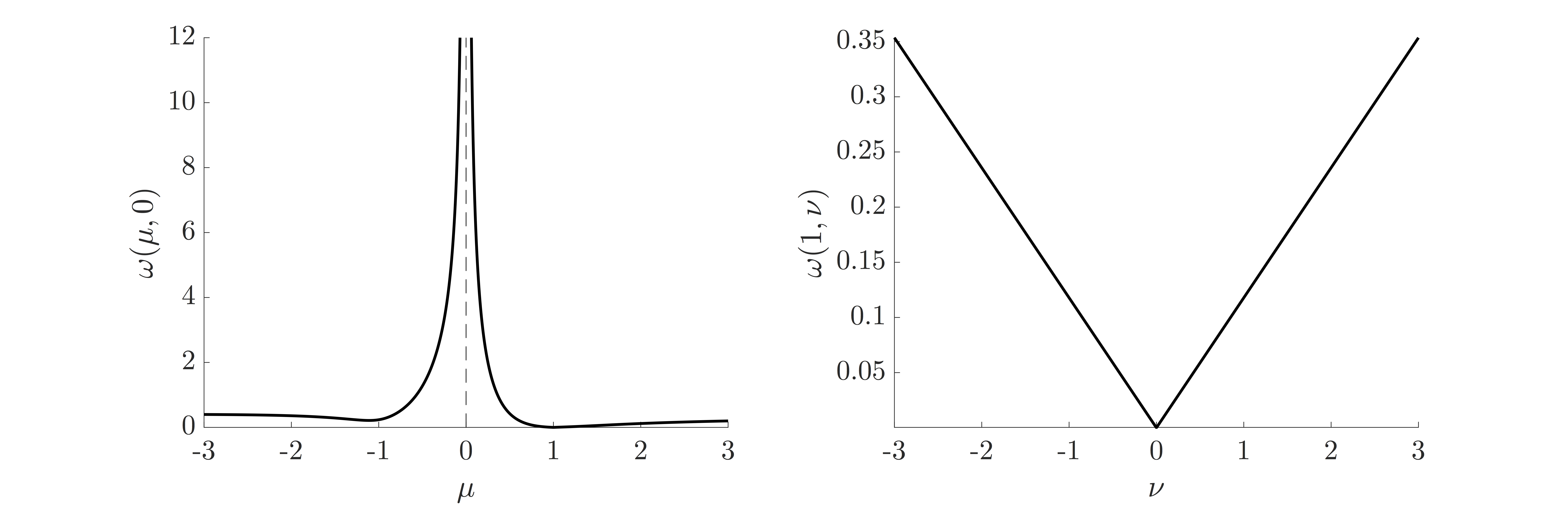
Although the difference between and can be significant, there are cases where they are identical. Some previous works have studied the problem of how close is to , e.g., [43, 9]. However, their assumptions do not apply to our matrix For our problem, when the linear system is consistent, since in this case, , or when , which is equivalent to , since implies that . In the example above, this occurs when (e.g., and ).
4 Numerical experiments
In this section we showcase the numerical performance of the discussed methods. A general framework for our proposed methods is summarized in Algorithm 1, where the main distinction among the stochastic gradient, Newton, and quasi-Newton methods is the choice of (see line 5). For the stochastic gradient method, , and for the stochastic Newton method, . For the stochastic quasi-Newton method, we will use the choices of described in Section 2 with and . To avoid large inversions when computing , we use the Woodbury formula to iteratively update this choice of as
| (13) |
and for ,
| (14) |
Update formulas (13) and (14) require an inversion of an matrix, but , which is the number of columns in , is assumed small.
Following most stopping criteria developed for stochastic optimization and stochastic learning methods [40, 5, 39], we rely on heuristic monitoring of and to determine early stopping for our methods. We consider three stopping criteria: a given maximum number of iterations, a certain tolerance on changes in , and a tolerance on the improvement in , see [12]. For the last two, we use
where is a given tolerance. Here, for some number , denotes the simple moving average . In our experiments we choose .
Next, we provide two experiments to illustrate our methods. In Experiment 1, we use a linear regression problem to illustrate various properties or our algorithms and
validate the theoretical results. In Experiment 2 we provide some results using a realistic example from machine learning.
Experiment 1
We consider a linear regression problem, where is a random matrix with elements drawn from a standard normal distribution. We let and , where the additive noise is also assumed to be standard normal. We choose to be a block Kaczmarz matrix with block size and utilize the harmonic sequence as the step size strategy. We select the inverse Hessian approximation using the update formula given in (13) and (14) with and start at a random initial guess . First, we compare the performance of the stochastic quasi-Newton and Newton methods. In Figure 2 we provide plots of relative errors. In the top left panel, the relative errors are computed as , where are stochastic quasi-Newton (SQN) iterates, and in the top right panel, the relative errors are computed as , where are stochastic Newton (SN) iterates. These plots illustrate convergence of SQN and SN iterates to and respectively, as proved in Section 3. Notice that stochastic Newton (red dashed line) exhibits much slower convergence to than the convergence of stochastic quasi-Newton (blue solid line) to . In fact, SN requires 20,000 iterations to reach a relative error of , while the SQN iterates reach a relative error of after 175 iterations. Moreover, it takes the stochastic quasi-Newton only 22 iterations to achieve a relative error of .

In the bottom panel of Figure 2, we provide reconstruction errors relative to the true solution for both methods, which demonstrates that SQN is faster than SN at providing a better approximation of the true solution. For this experiment the relative error between and is We omit the results for the stochastic gradient method due to poor performance. It is worth noting that the moderate size of this problem still allows one to use a QR solver (e.g., Matlab’s “backslash”) to solve the LS problem, which takes about seconds whereas SQN requires about seconds to run iterations.
Last, we investigate the performance of four different choices of : (i) Block Kaczmarz, which is the generalized Kaczmarz method with and uniformly to create blocks of the same size, (ii) Kaczmarz, which is similar to the generalized Kaczmarz method with but instead of a preset partitioning of the matrix into matrices this method samples columns of randomly at each iteration to generate , (iii) Sparse Rademacher with , and (iv) Sparse Random with . These choices of are defined on page 2. In Figure 3, we provide the function values with respect to the number of row accesses of , since row accesses of may be the computational bottle neck for large problems. We observe that all choices of perform similarly, with Kaczmarz and block Kaczmarz having a slight advantage. The performance of the stochastic quasi-Newton method is highly dependent on the underlying problem (e.g., structures in the matrix and vector ) and the realizations of . Empirically, using regression data sets from the UCI Machine Learning Repository [28], we observe best performances with block Kaczmarz and sparse Rademacher (data not shown).

Experiment 2
Next, we investigate the use of our stochastic quasi-Newton method for solving large linear LS problems that arise in extreme learning machines (ELMs). ELM is a machine learning technique that uses random hidden nodes or neurons in a feedforward network to mimic biological learning techniques. The literature on ELM in the machine learning community is vast, with cited benefits that include higher scalability, less computational complexity, no requirement of tuning, and smaller training errors than generic machine learning techniques. ELM is commonly used for clustering, regression, and classification. Full details and comparisons are beyond the scope of this paper, and we refer the interested reader to papers such as [21, 19, 22, 24, 23, 20] and references therein.
At the core of ELM is a very large and potentially dynamically growing linear regression problem. In this experiment, we investigate the use of stochastic algorithms for efficiently solving these LS problems. In particular, we consider the problem of handwritten digit classification using the “MNIST” database [7], which contains 60,000 training images and 10,000 testing images of handwritten digits ranging from 0 to 9. Each image is pixels and converted into a vector (e.g., corresponding to 784 features).
We begin with a brief description of the classification problem for the MNIST dataset. Suppose we are given a set of examples in the form of a training set
where and takes values from the set of classes . Consider an ELM with a hidden layer of nodes, then the goal is to solve a LS problem of the form,
| (15) |
where the hidden-layer output matrix is defined as
with being the output (row) vector of the hidden layer with respect to the input , where contains the desired output weights for class , and the training data target matrix takes entries
For this example, can be interpreted as a map from the image pixel space to the -dimensional hidden-layer feature space. Although various activation functions could be used, we employ a standard choice of sigmoid additive hidden nodes with
where all of the hidden-node parameters are randomly generated based on a uniform distribution [22]. For our experiments, we set the number of hidden neurons to be .
The main computational work of ELM is to solve (15). Regularized or constrained solutions have been investigated (e.g., [22, 29, 2]). However, our focus will be on solving the unconstrained LS problem efficiently and for very large sets of training data. In order to generate larger datasets, we performed multiple random rotations of the original 60,000 training images. More specifically, each image was rotated by degrees, where is a random number drawn from a beta distribution with shape parameters equal to . In our experiments, we consider up to random rotations per image, resulting in up to 900,000 training images. Notice that as the number of training images increases, the number of rows of increases accordingly, while the number of columns remains the same.
We consider three approaches to solve (15) and compare CPU timings. In the original implementation of ELM [24, 23], the LS solution was computed as where is the Moore-Penrose pseudoinverse of We denote this approach “PINV”. Another approach to solve large (often sparse) LS problems is to use an iterative method such as LSQR [35, 34], but since the LS problem needs to be solved for multiple right-hand sides (here, 10 solves), we use a global least squares method (Gl-LSQR) [42] with a maximum of 50 iterations and a residual tolerance of . It was experimentally shown in [42] that Gl-LSQR is more effective and less expensive than LSQR applied to each right hand side. We use our stochastic quasi-Newton (SQN) method where corresponds to the sparse Rademacher matrix with and . We use a maximum number of iterations of 1,000, a stopping tolerance of and an initial guess of . Since the matrices only depend on and SQN can be applied to multiple right hand sides simultaneously.
Each LS solver is repeated 20 times in Matlab R2015b on a MacBook Pro with 2.9 GHz Intel Core i7 and 8G memory, and in Figure 4, we provide the median and 5th–95th percentiles of the CPU times vs. the number of training images (e.g., number of rows in ). It is evident that for smaller training sets, all three methods perform similarly, but as the number of training images increases, SQN quickly surpasses PINV and Gl-LSQR in terms of faster CPU time. For various numbers of training data, we provide in Table 1 the mean and standard deviation of the relative reconstruction error for the SQN estimate, , and of the number of SQN iterations, . Our results demonstrate that SQN does not necessarily provide the most accurate solutions, however, it can be used to achieve sufficiently good solutions in an efficient manner.

| 0.2705 | 0.2665 | 0.2456 | 0.2649 | 0.2568 | |
| 632 219 | 675 227 | 706 194 | 631 196 | 663 180 |
Next we test the performance of these estimates for classification of the MNIST testing dataset. That is, once computed, the output weights can be used to classify images in the following way. For each test image, the predicted class is given by
In Figure 5 we provide a visualization of the computed classifications for the 10,000 testing images, where accuracy values in the titles are calculated as where is the number of misclassified images. An accuracy value that is close to corresponds to a good performance of the classifier. These results correspond to training on 60,000 images, and the testing set was sorted by class for easier visualization. Notice that in Figure 5 the misclassified images are almost identical for all three methods, and the classification accuracy for SQN is only slightly smaller than that of PINV and Gl-LSQR. Thus, we have shown that our SQN method can achieve comparable classification performance as PINV and GL-LSQR with much faster learning speed.

It is worth noting that the matrices considered here, though large, can still be loaded into memory. For problems where this is not the case (e.g., data too large or being dynamically generated [45]), PINV and Gl-LSQR would not be feasible, while SQN could still be used.
5 Conclusions
In this paper we introduced a stochastic Newton and a stochastic quasi-Newton method for solving very large linear least-squares problems. New theoretical results show that under mild regularity conditions on the distributions, the stochastic quasi-Newton iterates converge to the unique LS solution , while the stochastic Newton iterates converge to a different estimator of which is still unbiased but is likely to have larger variance. We provide implementation details for choices of random variables , step length parameters , and stochastic inverse Hessian approximations . Our numerical experiments validate our theory and also show the potential benefits of these methods for machine learning applications where the data sets of interests are typically extremely large. Furthermore, by allowing sparse distributions, our approaches can handle scenarios where the entire matrix is not available or full matrix-vector multiplications with are not feasible.
This work opens the doors to a plethora of new methods, advancements, and implementations for stochastic Newton and quasi-Newton methods. Current work includes the development of limited-memory quasi-Newton methods to reduce the storage and updating costs for the sequence of matrices, adaptive choices of that can exploit matrix properties, efficient parallel implementations, and extensions to nonlinear problems.
Acknowledgement: The authors are grateful to Qi Long for initial discussions and Arvind Saibaba for helpful comments that have improved the manuscript. We are also grateful to Eldad Haber for pointing us to the ELM problem and to the Institute for Mathematics and its Applications for nurturing this research collaboration.
6 Appendix
6.1 Proof of Theorem 3.2
(i) Let and assume that has the same distribution as . Then,
and therefore . Furthermore,
and therefore iff a.s., which happens iff a.s., in which case
This implies , and thus is defined and SPD.
(ii) Note that
| (16) |
where Therefore,
and there are positive constants and such that
for all . Since and are independent and , it follows that for all . This together with (16) implies that for all .
(iii) By definition,
and therefore
Since this residual vector is orthogonal to the column space of , (16) leads to
| (17) |
Let , then
and therefore
| (18) |
Equations (17) and (18) lead to
subtracting from both sides yields
Define Since
for any , it follows that is a decreasing and convergence sequence to some . Define and , then
| (19) | |||||
and also
Theorem 3.1 now implies that converges a.s. and since converges to a nonzero value, it follows that also converges a.s. The final step is to show that . It follows from (19) that
for any . Therefore,
Since a.s., it follows that for almost all there is a subsequence such that which also implies
and therefore, since converges a.s., we also have . Hence, .
6.2 Proof of Theorem 3.3
The proof is a slight modification of that of Theorem 3.2. Define . (i) Let Since it follows that is semi-positive definite, and therefore so is . Since is symmetric, is symmetric. Let Using properties of the pseudoinverse gives
where equality holds iff a.s., and since and is full column-rank, it follows that . Hence is SPD.
(ii) Note that
| (20) |
where . Therefore
and since is an orthogonal projection matrix, it follows that
This then leads to
which implies that and for all .
(iii) The idea is again to use the quasimartingale convergence theorem. Since and are independent,
| (21) | |||||
To put a bound on the second term of (21) we use again the fact that is a projection matrix to obtain:
| (22) |
where . Therefore, equation (21) can be bounded as
which yields
| (23) |
Let The sequence converges to some because . Define and multiply both sides of (23) by . We obtain
| (24) |
Define . Then,
Since the series converges and therefore converges a.s. by Theorem 3.1. But since converges to a nonzero value, it also follows that converges a.s. The final step is to show that in fact converges to zero. Rearranging the terms and taking the expected value of both sides of (24) yields
Since and , it follows that for some subsequence , and therefore we also have . By Fatou’s lemma:
It follows that a.s. and since converges a.s., this implies and therefore .
References
- [1] D. Achlioptas. Database-friendly random projections: Johnson-Lindenstrauss with binary coins. Journal of Computer and System Sciences, 66(4):671–687, 2003.
- [2] Z. Bai, G.-B. Huang, D. Wang, H. Wang, and M. B. Westover. Sparse extreme learning machine for classification. IEEE Transactions on Cybernetics, 44(10):1858–1870, 2014.
- [3] A. Benveniste, S. Wilson, M. Metivier, and P. Priouret. Adaptive Algorithms and Stochastic Approximations. Stochastic Modelling and Applied Probability. Springer, New York, 2012.
- [4] L. Bottou. Online Learning in Neural Networks, chapter 2. Online learning and stochastic approximations, pages 9–42. Cambridge University Press, 1998.
- [5] L. Bottou, F. E. Curtis, and J. Nocedal. Optimization methods for large-scale machine learning. arXiv preprint arXiv:1606.04838, 2016.
- [6] C. Boutsidis and A. Gittens. Improved matrix algorithms via the subsampled randomized Hadamard transform. arXiv preprint arXiv:1204.0062, 2012.
- [7] L. Deng. The MNIST database of handwritten digit images for machine learning research [best of the web]. IEEE Signal Processing Magazine, 29(6):141–142, 2012.
- [8] P. S. R. Diniz. Adaptive filtering. Springer, New York, 1997.
- [9] P. Drineas, M. W. Mahoney, S. Muthukrishnan, and T. Sarlós. Faster least squares approximation. Numerische Mathematik, 117(2):219–249, 2011.
- [10] J. Fan, Y. Liao, and H. Liu. An overview of the estimation of large covariance and precision matrices. The Econometrics Journal, 19(1):C1–C32, 2016.
- [11] D. L. R. Fisk. Quasi-Martingales and Stochastic Integrals. Department of Mathematics Research Monograph. Kent State University, Department of Mathematics, 1963.
- [12] P. E. Gill, W. Murray, and M. H. Wright. Practical Optimization. Emerald, Bingley, 2007.
- [13] R. M. Gower, D. Goldfarb, and P. Richtárik. Stochastic block BFGS: Squeezing more curvature out of data. arXiv preprint arXiv:1603.09649, 2016.
- [14] R. M. Gower and P. Richtárik. Randomized iterative methods for linear systems. SIAM Journal on Matrix Analysis and Applications, 36(4):1660–1690, 2015.
- [15] R. M. Gower and P. Richtárik. Randomized quasi-Newton updates are linearly convergent matrix inversion algorithms. arXiv preprint arXiv:1602.01768, 2016.
- [16] E. Haber, M. Chung, and F. Herrmann. An effective method for parameter estimation with PDE constraints with multiple right-hand sides. SIAM Journal on Optimization, 22(3):739–757, 2012.
- [17] P. C. Hansen, V. Pereyra, and G. Scherer. Least Squares Data Fitting with Applications. John Hopkins University Press, Baltimore, 2012.
- [18] A. Hedayat and W. D. Wallis. Hadamard matrices and their applications. The Annals of Statistics, 6(6):1184–1238, 1978.
- [19] G. Huang, G.-B. Huang, S. Song, and K. You. Trends in extreme learning machines: A review. Neural Networks, 61:32–48, 2015.
- [20] G.-B. Huang, Z. Bai, L. L. C. Kasun, and C. M. Vong. Local receptive fields based extreme learning machine. IEEE Computational Intelligence Magazine, 10(2):18–29, 2015.
- [21] G.-B. Huang, D. H. Wang, and Y. Lan. Extreme learning machines: a survey. International Journal of Machine Learning and Cybernetics, 2(2):107–122, 2011.
- [22] G.-B. Huang, H. Zhou, X. Ding, and R. Zhang. Extreme learning machine for regression and multiclass classification. IEEE Transactions on Systems, Man, and Cybernetics, Part B (Cybernetics), 42(2):513–529, 2012.
- [23] G.-B. Huang, Q.-Y. Zhu, and C.-K. Siew. Extreme learning machine: a new learning scheme of feedforward neural networks. In Neural Networks, 2004. Proceedings. 2004 IEEE International Joint Conference on, volume 2, pages 985–990. IEEE, 2004.
- [24] G.-B. Huang, Q.-Y. Zhu, and C.-K. Siew. Extreme learning machine: theory and applications. Neurocomputing, 70(1):489–501, 2006.
- [25] S. Kaczmarz. Angenäherte Auflösung von Systemen linearer Gleichungen. Bulletin International de l’Académie Polonaise des Sciences et des Lettres. Classe des Sciences Mathématiques et Naturelles. Série A, Sciences Mathématiques, 35:335–357, 1937.
- [26] H. J. Kushner and G. G. Yin. Stochastic Approximation Algorithms and Applications. Springer, New York, 1997.
- [27] E. B. Le, A. Myers, and T. Bui-Thanh. A randomized misfit approach for data reduction in large-scale inverse problems. arXiv preprint arXiv:1603.01562, 2016.
- [28] M. LLC. Machine Learning Repository, Center for Machine Learning and Intelligent Systems, University of California, Irvine, 2017.
- [29] J. Luo, C.-M. Vong, and P.-K. Wong. Sparse Bayesian extreme learning machine for multi-classification. IEEE Transactions on Neural Networks and Learning Systems, 25(4):836–843, 2014.
- [30] M. Métivier. Semimartingales: A Course on Stochastic Processes. De Gruyter studies in mathematics. XI, 1982.
- [31] D. Needell, N. Srebro, and R. Ward. Stochastic gradient descent, weighted sampling, and the randomized Kaczmarz algorithm. Mathematical Programming, 155(1-2):549–573, 2016.
- [32] D. Needell and J. A. Tropp. Paved with good intentions: analysis of a randomized block Kaczmarz method. Linear Algebra and its Applications, 441:199–221, 2014.
- [33] J. Nocedal and S. J. Wright. Numerical Optimization. Springer, New York, second edition edition, 2006.
- [34] C. C. Paige and M. A. Saunders. Algorithm 583, LSQR: Sparse linear equations and least-squares problems. ACM Transactions on Mathematical Software, 8(2):195–209, 1982.
- [35] C. C. Paige and M. A. Saunders. LSQR: An algorithm for sparse linear equations and sparse least squares. ACM Transactions on Mathematical Software, 8(1):43–71, 1982.
- [36] M. Pilanci and M. J. Wainwright. Iterative Hessian sketch: Fast and accurate solution approximation for constrained least-squares. Journal of Machine Learning Research, 17(53):1–38, 2016.
- [37] H. Robbins and S. Monro. A stochastic approximation method. The annals of mathematical statistics, pages 400–407, 1951.
- [38] H. Robbins and D. Siegmund. A convergence theorem for non negative almost supermartingales and some applications. In Herbert Robbins Selected Papers, pages 111–135. Springer, 1985.
- [39] A. Shapiro, D. Dentcheva, and A. Ruszczynski. Lectures on Stochastic Programming: Modeling and Theory, volume 16. SIAM, Philadelphia, 2014.
- [40] J. C. Spall. Introduction to stochastic search and optimization: estimation, simulation, and control, volume 65. John Wiley & Sons, Hoboken, 2005.
- [41] T. Strohmer and R. Vershynin. A randomized Kaczmarz algorithm with exponential convergence. Journal of Fourier Analysis and Applications, 15(2):262–278, 2009.
- [42] F. Toutounian and S. Karimi. Global least squares method (Gl-LSQR) for solving general linear systems with several right-hand sides. Applied Mathematics and Computation, 178(2):452–460, 2006.
- [43] D. P. Woodruff. Sketching as a tool for numerical linear algebra. Foundations and Trends® in Theoretical Computer Science, 10(1–2):1–158, 2014.
- [44] P. Xu, J. Yang, F. Roosta-Khorasani, C. Ré, and M. W. Mahoney. Sub-sampled Newton methods with non-uniform sampling. arXiv preprint arXiv:1607.00559, 2016.
- [45] J. Zhao, Z. Wang, and D. S. Park. Online sequential extreme learning machine with forgetting mechanism. Neurocomputing, 87:79–89, 2012.