Enhanced quantum sensing with multi-level structures of trapped ions
Abstract
We present a method of enhanced sensing of AC magnetic fields. The method is based on the construction of a robust qubit by the application of continuous driving fields. Specifically, magnetic noise and power fluctuations of the driving fields do not operate within the robust qubit subspace, and hence, robustness to both external and controller noise is achieved. The scheme is applicable to either a single ion or an ensemble of ions. We consider trapped-ion based implementation via the dipole transitions, which is relevant for several types of ions, such as the , , and the ions. Taking experimental errors into account, we conclude that the coherence time of the robust qubit can be improved by up to orders of magnitude compared to the coherence time of the bare states. We show how the robust qubit can be utilized for the task of sensing AC magnetic fields in the range MHz with an improvement of orders of magnitude of the sensitivity. In addition, we present a microwave based sensing scheme that is suitable for ions with a hyperfine structure, such as the ,,,,,,, and the ions. This scheme enables the enhanced sensing of high frequency fields at the GHz level.
I Introduction
Quantum sensing [1, 2] and metrology [5, 4, 3] exploit physical laws governing individual quantum systems or correlations between systems to perform detection at the limits of precision and resolution. Improving the precision of sensing of weak electromagnetic fields is a prime goal in this field. The limit of most quantum sensing protocols scales as [6, 7, 8], where is the coherence time. The coherence time for many experimental platforms is limited by ambient magnetic field fluctuations. Consequently, dynamical decoupling methods, designed to prolong the coherence time, are incorporated into the sensing schemes in order to improve the sensing precision.
Pulsed dynamical decoupling [9, 10, 11] is a useful tool for prolonging the coherence time [12, 13, 14, 15, 16, 17, 18, 19]. Diminishing both external and controller noise, however, requires very rapid and composite pulse sequences [20, 21, 22, 23, 24] and consequently uses a considerable amount of power [25]. In addition, a major drawback of incorporating state-of-the-art pulsed dynamical decoupling in sensing schemes is that usually, the frequency of the pulses must coincide with the frequency of the sensed field; the time interval between the pulses should be fixed to , where is the frequency of the signal. Hence, this approach can not be used to integrate dynamical decoupling in the sensing of high frequency fields.
Sensing of high frequency signals is of great importance, especially in the case of classical fields sensing [26, 29, 28, 27], in the detection of electron spins in solids [31, 30, 32] and NMR [33]. As the method of choice for this regime is relaxometry, the sensitivity is limited by the coherence time, and specifically by the pure dephasing time, , since no dynamical decoupling schemes are employed.
Continuous dynamical decoupling [34, 35, 36, 37, 38, 39, 40, 25, 41, 42, 43, 44] provides a different approach for achieving robustness to both external and controller noise [45, 46]. Ultra-sensitive sensing that is based on continuous dynamical decoupling was demonstrated in [47], utilising a four level configuration. Remarkably, continuous dynamical decoupling can be elegantly incorporated in the sensing of high frequency fields [48, 49]


In this paper, we elaborate on the work presented in [46] with the focus on AC magnetic field sensing. We show that utillizing a compact constuction of a protected qubit subspace that requires only two (detuned) optical driving fields (compared to five in [46]), results in a protected qubit that can indeed be used as a sensor of AC magnetic fields in the range MHz with enhanced sensitivity. In addition, we present a microwave based sensing scheme that is suitable for ions with a hyperfine structure. In this scheme a robust qubit is constructed within the ground state manifold of the ion. We show that this construction enables the enhanced sensing of high frequency fields, where the frequency of the signal corresponds to a transition between two bare states from two different hyperfine levels, which is of the order of the hyperfine splitting. The sensed frequency, at the GHz level, is tuned by the static magnetic field.
The paper is organized as follows. We begin in section II with a general definition of a protected qubit subspace. In section III we discuss the realization of a protected qubit subspace with trapped ions. We start with a review of the on-resonance construction [46], and then present the new compact construction. In section IV we analyze the performance of the compact construction under realistic experimental errors and sources of noise. We continue with suggestions for other possible constructions in section V, and for completeness, in section VI we show how the protected qubit can be manipulated [46]. In section VII we discuss the implications of the scheme for sensing AC fields, and in section VIII we present the new microwave based construction. Finally, we end in section IX with the conclusions.
II Protected qubit subspace
We start with an explicit definition of a protected qubit subspace [46]. Let us denote the protected qubit states by . In what follows is the (continuous) driving Hamiltonian, is the Hilbert subspace of the protected qubit, and is the complementary Hilbert space, that is, . We define the protected qubit subspace by (See Fig. 1)
| (1) | |||||
| (2) |
The first equation ensures that magnetic noise does not operate within the protected qubit subspace; the noise can only cause transitions between a protected state and a state in the complementary subspace. We assume (by construction) that the energy of all states in is far from the energy of the states in . More specifically, we assume that , where () is an eigenvalue of an eigenstate in (), is much larger than the characteristic frequency of the noise, as in this case the lifetime would be inversely proportional to the power spectrum of the noise at . This ensures that the rate of transitions from to due to magnetic noise is negligible.
The second equation indicates that the protected states do not collect a relative dynamical phase due to , and are therefore immune to noise originating from . Power fluctuations of the driving fields result in identical energy fluctuations of the protected states.
To summarize, the first equation ensures that the protected states are immune to external noise, while the second equation ensures that the protected states are also immune to controller noise.
III Implementation with trapped-ions

We consider ions such as the , , and the ions, that have a typical level structure, as shown in Fig. 2. Because the lifetime of the states is second, we utilize their subspace for the construction of the protected qubit subspace. For simplicity we will use the notation , and . The states,
| (3) | |||||
| (4) |
fulfill the first condition of a protected qubit subspace, which is given by Eq. 1, . The second condition, which is given by Eq. 2, is fulfilled by constructing the driving fields such that (). This can be obtained by coupling the (bare) states to the states on resonance in two configurations (see Fig. 3).
The driving Hamiltonian of the two systems (in the interaction picture (IP) with respect to the energies of the bare states, and taking the rotating-wave approximation (RWA)) is given by
| (5) | |||||
where is the Rabi frequency of the driving fields. The states and are the eigenstates of with a zero eigenvalue. The eigenvalues of the remaining four eigenstates are equal to (See Fig. 3).
The construction can be elucidated by considering one of the systems. In the basis the driving Hamiltonian of the system is given by
| (6) |
Hence, the dark state is decoupled from the bright state , and the excited state (See Fig. 4). In the basis of the dressed states we have that
| (7) |
where , and .

While for the first system the ratio between the Rabi frequencies of the and fields is , for the second system the ratio between the Rabi frequencies of the and fields is . A priori, it therefore seems that four driving fields are required, two fields for each system. However, the Clebsch-Gordan coefficients, , of the transitions, fulfill the following relations (See Fig. 5).
| (8) |
This means that only two driving fields (a field and a field) with an equal Rabi frequency are required for the construction of the two protected qubit states. In this case, in the first system we have a (blue) one-photon detuning and in the second system of we have a (red) one-photon detuning of . These one-photon detunings will not affect the protected qubit states and will only modify the eigenstates in and their energies, which will be slightly lower. For a static magnetic field, such that MHz (which should be large enough to mitigate and noise), and a Rabi frequency of MHz (), the protected qubit states remain well decoupled from the bright states. In this case the dressed states and are modified with an amplitude mixing of between them, and their energies are shifted by an energy shift of . In appendix A we give a detailed description of the protected qubit construction. We consider this compact construction of the protected qubit subspace in subsequent sections.

IV Error estimation
In this section we consider possible experimental errors and sources of noise, and analyze their effect on the lifetime and the coherence time of the protected qubit.
IV.1 Noise and systematic shifts of the magnetic field
Because the magnetic noise couples between a protected state and a non-protected state, in first order, the noise induces a longitudinal relaxation (decay) rate of , where is the power spectrum of the noise. A large enough ensures that the longitudinal relaxation rate is negligible (). In our construction we consider a Rabi frequency of MHz, which implies that for a typical magnetic noise is negligible.
In second order, a Zeeman shift of results in an energy gap of between the protected qubit states (see Appendix B). For the energy gap is . Even with kHz, which corresponds to a strong magnetic noise (s) or a large systematic shift, this implies a limit of an improvement of orders of magnitude in the coherence time.
In addition, the Zeeman shift of , creates a two photon detuning, which results in an amplitude mixing between a protected state and an excited state , where the probability to populate the excited states is (See Fig. 6). This implies a limit on the lifetime of the protected qubit due to the strong decay rate of the states, MHz. For KHz and MHz the lifetime is limited to sec, which corresponds to a limit of orders of magnitude improvement of the coherence time. Stronger driving fields of GHz result in sec, which corresponds to a limit of orders of magnitude improvement in the coherence time.
IV.2 Relative amplitude error
In a relative amplitude error, the amplitude ratio between the two fields (of the systems) is larger/smaller then its ideal value, and for one of the fields we have that . As a result, the amplitudes of the bare states in are modified by . That is, a relative amplitude error results in a mixing between a protected state and the bright state (See Fig. 6). In this case, the probability of being in the excited state is zero, but because is modified to , scale as . However, while the coupling rate between and is , the coupling rate between and is . As , we have that the uncertainty of the energy gap between the two robust states scales as (See Appendix B). This limits the coherence time to An implies a limit of an improvement of orders of magnitude in the coherence time.
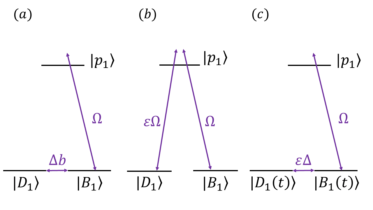
IV.3 Polarization errors
Here we assume that a fraction () of a beam is a beam and vice versa. Hence, we have that (for the state for example) the Rabi frequency of the field is , and the Rabi frequency of the field is , where and is the Landé g factor of the level. In this case, the dark state of the system is a time dependent state, which is given (up to normalization) by Due to the time dependence of the Rabi frequencies, and , there is an effective coupling rate between the instantaneous states and , which is . This results in a non-zero probability to be in the excited state , which is . For and , , and therefore does not limit the lifetime. In addition, we also have that , and the coherence time is not affected. For more details, see Appendix B.
V Alternative constructions
There are two additional possibilities for the construction of the protected qubit subspace with optical fields. The first alternative is to couple the states to the states instead of the states. In this case the driving fields corresponds to two configurations, but the resulting protected qubit states, and are the same. The advantage of this construction is that here, experimental errors can lead to a probability of populating the states rather than the states, which does not limit the lifetime of the protected qubit. However, this requires a sufficiently strong coupling rate between the states and the states such that an energy gap of kHz is formed between the protected qubit states and non-protected states.
Yet another alternative is to use the subspace as the protected qubit subspace. Similar to the constructions with the states, the Clebsch-Gordan coefficients of the transitions imply that only two driving fields (a field and a field) with an equal Rabi frequency are required for the construction of the two protected qubit states. As for the construction, this configuration results in the two dark (zero eigenvalue) eigenstates and , where in this case . Hence, and fulfill both Eq. 1 and Eq. 2, and constitute a protected qubit subspace.
VI Initialization and single qubit gates

.
VI.1 Initialization
Initialization may be achieved by the application of optical pumping to the state, followed by a STIRAP procedure, which results in the state. At this point, the Rabi frequencies of the driving fields are fixed and remain so during the whole experiment. Measurements are performed by a reversed process.
An alternative method is to perform a direct gate from an state to one of the states. However, this requires two phase-matched lasers.
VI.2 Direct gate
A gate can be implemented with a microwave field, which is set to apply a gate in the bare states basis (or a with a relative phase shift of ), on resonance with the (Zeeman) energy gap between the sub-levels (See Fig. 7) and corresponds to
| (9) |
Moving to the IP, with respect to the bare energy gaps (and taking the RWA) leads to . In the robust states basis the bare states’ operates within the protected subspace , and within the complementary subspace , but does not couple between states in and states in . In the protected qubit subspace , this results in a operator which is given by
| (10) |
VI.3 gate
An effective gate can be realized by a Raman transition between the bare and states (via one of the states, See Fig. 7). The (IP) Hamiltonian of the Raman transition is
| (11) | |||||
Moving to the dressed states basis and to the IP with respect to the energies of the dressed states we obtain
| (12) | |||||
where off-resonant coupling terms between states within have been neglected. Taking results in the effective Hamiltonian
| (13) |
Together with the gate, a
gate, and hence, any single qubit unitary operation,
can be performed.

.
VII Sensing
The operation of the gate can be used for the task of sensing AC magnetic fields. An AC signal whose frequency is on resonance with the Zeeman energy gap between the bare states will induce rotations of the protected qubit. In this case the sensitivity scales as , where is the prolonged coherence time of the protected qubit. The range of frequencies that can be detected with this scheme is MHz. The lower limit is determined by the energy gap of the bare states, which should be large enough in order to mitigate magnetic and noise. The power spectrum of the noise at MHz may not be negligible and hence, transverse noise may induce longitudinal relaxation of the protected qubit. The upper limit is fixed by the experimental ability to apply a strong static magnetic field. For typical ion traps, the upper bound corresponds to a Zeeman splitting of MHz. Since the phase of an external signal is usually random with respect to the driving fields, the sensed Rabi frequency of the signal is attenuated by a factor of . This is due to the fact that only a polarization induces a rotation in the protected qubit subspace.
VIII Implementation with hyperfine structure
Here we consider ions with an hyperfine structure, where the ground state manifold has two hyperfine levels, and . For example, the and ions have and ground states, the ion has and , the ion has and ground states, and the ion has and ground states. For each ion, the Landé g-factors of the ground states are of the same magnitude, that is, . This enables the on-resonance driving of both levels by a single driving field, and hence the construction of a protected qubit subspace by a single on-resonance driving field. If the on-resonance driving field is polarized along the axis, the Hamiltonian of ions with an and ground states, for example, is given by
| (14) |
where () and () are the and operators, which operate on the () levels respectively. In the IP we have that
| (15) |
and so the dressed eigenstates of the driving field are the eigenstates, which fulfill Eq. 1 and are robust to magnetic noise. The eigevalues of the dressed and states are and respectively. Choosing two eigenstates, one from each level, that have the same eigenvalue (i.e., the same energy) ensures that these two states also fulfill Eq. 2, and are therefore also robust to power fluctuations of the driving field (See Fig. VIII).
Because the protected qubit states have the same energy, their on-resonance coupling frequency is a frequency of an allowed transition between two bare states that have a non-zero amplitude component in the dressed states, and up to the Zeeman splitting corresponds to the hyperfine splitting. Denote by the frequency which corresponds to the hyperfine splitting, and consider the two eigenstates with the zero eigenvalue as the protected qubit states, and . The driving field
| (16) |
which is on resonance with the transition corresponds to the on resonance coupling between the two protected states. In the first IP with respect to the Zeeman splitting
| (17) |
where all coupling terms within , and off-resonance coupling terms between a state in and a state in have been neglected. Moving now to the IP with respect to the hyperfine splitting results in
| (18) |
For ions with an level, such as the , and the ions, the driving field will operate only on the level. The protected qubit states are then seen to be the bare state and the dressed eigenstate with the zero eigenvalue of the level (which is the state.
The hyperfine ground states energy gap in these ions is GHz, and hence, our scheme provides a method for the enhanced sensing of high frequency signals. While with common high frequency sensing methods, the obtained sensitivity is limited by the pure dephasing time , in our method the sensitivity is limited by the prolonged coherence time.
IX Conclusions
This paper describes a scheme for the construction of a protected qubit subspace. Specifically, we present a simplified and compact optical implementation of the scheme, which is of relevance to several types of ions and can be used for enhanced sensing of AC magnetic fields. The scheme is applicable to either a single ion or an ensemble of ions. Taking experimental errors into account, we predict an improvement of 2 orders of magnitude in sensitivity. We also describe a new implementation of the scheme that is suitable for ions with hyperfine structure, where a protected qubit subspace is constructed within the ground state manifold by the application of a single microwave field. Importantly, this implementation enables the enhanced sensing of high frequency fields at the GHz level, which corresponds to the energy gap between the hyperfine levels. Owing to the high resolution of the scheme, the implication of this method for wireless communication [50] may prove to be very significant. Moreover, this method could also be used to improve the coupling to quantum systems [37], and to improve the resolution of classical fields sensing [26, 29, 28, 27].
X Acknowledgements
A. R. acknowledges the support of the Israel Science Foundation(grant no. 1500/13), the support of the European commission (STReP EQUAM Grant Agreement No. 323714), EU Project DIADEMS, the Marie Curie Career Integration Grant (CIG) IonQuanSense(321798), the Niedersachsen-Israeli Research Cooperation Program and DIP program (FO 703/2-1). This work is partially supported by the US Army Research Office under Contract W911NF-15-1-0250. This project has received funding from the European Union as Horizon 2020 research and innovation programme under grant agreement No 667192.
M.D. appreciates generous support through the The Danish Council for Independent Research, Sapere Aude DFF-Advanced Grant; and the VELUX Foundations.
Appendix A
In this section we describe the construction of the protected qubit subspace in detail.
A.1 Ideal construction
Here we assume that for each system we have two independent driving fields that operate only on the transitions within the system. Denote by and the energy gap between the and levels, and the amplitude of the static magnetic field ( here corresponds to ). Note that the Landé g-factor of the and levels is and respectively. We then have that
| (19) |
The Hamiltonians of the on-resonance driving fields are therefore given by
| (20) | |||||
and the total Hamiltonian is
| (21) |
Moving to the IP with respect to , and making the RWA we arrive at Eq. (5),
| (22) | |||||
In the basis the Hamiltonian is given by
| (23) |
where only the bright states are coupled to the excited states. In the basis of its eigenstates, reads as
| (24) | |||||
where , , , and .
A.2 Compact construction
The relation between the Clebsch-Gordan coefficients of the transitions, given by Eq. 8, suggest that the protected qubit subspace can be constructed by only two driving fields, which operate on both systems and have the same Rabi frequency. We set the driving frequencies of the and fields to and , and define . In this case, the Hamiltonians of the driving fields are given by
| (25) | |||||
Moving to the IP with respect to , and making the RWA we obtain
| (26) | |||||
where is the one-photon detunings of the driving fields. We consider the regime where , which means that the ideal and eigenstates are slightly mixed, with an amplitude mixing of , and their energies are shifted by an energy shift of . The protected qubit states remain exactly the same and well decoupled from the bright and excited states.
Appendix B
In this section we derive the results presented in Sec. IV. We consider the compact construction of the protected qubit subspace.
B.1 Magnetic shift
A magnetic shift affects both and levels, and is described by the Hamiltonian
| (27) |
where, () operates on the () states. Adding to and moving to the IP results in
| (28) | |||||
| (29) |
In second order of , the energies of the protected and states are modified to and respectively.
Because the magnetic shift couples between the protected (dark) states and the bright states, and the driving fields couple between the bright states and the excited states, the magnetic shift also results in a small amplitude mixing of between a protected state and an excited state.
B.2 Relative amplitude
We consider the case where the amplitude of one of the driving fields, the field for example, is instead of . The Hamiltonian in the IP is therefore modified to
| (30) | |||||
which in the basis is given by
| (31) | |||||
The protected states are therefore modified to
| (32) |
In first order of , for both states . In second order of we find that , which limits the coherence time to
B.3 Polarization error
Here we assume that a fraction of a beam is a beam and vice versa. Hence, we find that, for the state for example, the Rabi frequency of the field is , and the Rabi frequency of the field is , where . The Hamiltonian in the IP and in the basis is given by
| (33) | |||||
The modified time-dependent robust states, are robust to magnetic noise and satisfy Eq. 1, . The dominant effect of polarization error is a non-zero probability to populate the excited states. Similar to adiabatic transfer, the time dependency of the driving fields results is a coupling between the instantaneous and states, which is . Hence the probability of populating the excited state is .
References
- [1] C. L. Degen, F. Reinhard, and P. Cappellaro. arXiv preprint, arXiv:1611.02427, 2016.
- [2] Dmitry Budker and Michael Romalis. Nature Physics 3, 227 (2007)
- [3] JJ Bollinger, Wayne M Itano, DJ Wineland, and DJ Heinzen. Phys. Rev. A 54, R4649(R) (1996)
- [4] Vittorio Giovannetti, Seth Lloyd, and Lorenzo Maccone. Science, 306 1330, (2004).
- [5] Vittorio Giovannetti, Seth Lloyd, and Lorenzo Maccone. Phys. Rev. Lett. 96, 010401 (2006)
- [6] WM Itano, JC Bergquist, JJ Bollinger, JM Gilligan, DJ Heinzen, FL Moore, MG Raizen, and DJ Wineland. Phys. Rev. A 47, 3554
- [7] Carl W Helstrom. Quantum detection and estimation theory. Journal of Statistical Physics, 1(2):231, 1969.
- [8] Alexander S Holevo. Probabilistic and statistical aspects of quantum theory, volume 1. Springer Science and Business Media, 2011.
- [9] E. L. Hahn, Phys. Rev. 80, 580 (1950).
- [10] H. Y. Carr and E. M. Purcell, Phys. Rev. 94, 630 (1954).
- [11] S. Meiboom and D. Gill, Rev. Sci. Instrum. 29, 688 (1958).
- [12] L. Viola and S. Lloyd, Phys. Rev. A 58, 2733 (1998).
- [13] M. J. Biercuk, H. Uys, A. P. VanDevender, N. Shiga, W. M. Itano, and J. J. Bollinger, Nature 458, 996 (2009).
- [14] J. Du, X. Rong, N. Zhao, Y. Wang, J. Yang and R. B. Liu Nature 461 1265 (2009).
- [15] G. de Lange, Z. H. Wang, D. Ristè, V. V. Dobrovitski, and R. Hanson Science 330, 60 (2010).
- [16] C. A. Ryan, J. S. Hodges, and D. G. Cory, Phys. Rev. Lett. 105, 200402 (2010).
- [17] B. Naydenov, F. Dolde, L. T. Hall, C. Shin, H. Fedder, L. C. L. Hollenberg, F. Jelezko, and J. Wrachtrup, Phys. Rev. B 83, 081201(R) (2011).
- [18] Z.-H. Wang, G. de Lange, D. Ristè, R. Hanson, and V. V. Dobrovitski, Phys. Rev. B 85, 155204 (2012).
- [19] N. Bar-Gill, L.M. Pham, A. Jarmola, D. Budker, and R.L. Walsworth, Nat. Commun. 4, 1743 (2012).
- [20] K. Khodjasteh and D. A. Lidar, Phys. Rev. Lett. 95, 180501(2005).
- [21] G. Uhrig, Phys. Rev. Lett. 98, 100504 (2007).
- [22] A. M. Souza, G. A. Álvarez, and D. Suter, Phys. Rev. Lett. 106, 240501 (2011).
- [23] Wen Yang, Zhen-Yu Wang, Ren-Bao Liu, Front. Phys. 6, 2 (2011).
- [24] D. Farfurnik, A. Jarmola, L. M. Pham, Z. H. Wang, V. V. Dobrovitski, R. L. Walsworth, D. Budker, and N. Bar-Gill, Phys. Rev. B 92, 060301(R) (2015).
- [25] Goren Gordon, Gershon Kurizki, and Daniel A. Lidar, Phys. Rev. Lett. 101, 010403 (2008).
- [26] M. Chipaux, L. Toraille, C. Larat, L. Morvan, S. Pezzagna, J. Meijer, and T. Debuisschert, Appl. Phys. Lett. 107, 233502 (2015).
- [27] Linbo Shao , Ruishan Liu , Mian Zhang , Anna V. Shneidman , Xavier Audier , Matthew Markham , Harpreet Dhillon , Daniel J. Twitchen , Yun-Feng Xiao , and Marko Loncar. Advanced optical materials, 4, 1075 (2016)
- [28] Linbo Shao, Mian Zhang, Matthew Markham, Andrew M. Edmonds, and Marko Lon?ar,Physical review applied 6, 064008 (2016)
- [29] S. Kolkowitz et. al., Science 347 1129 (2015)
- [30] LT Hall et. al., Nature Communications 7, 10211, (2016).
- [31] A. O. Sushkov et. al., Nano Lett. 14, 6443, (2014).
- [32] Dominik Schmid-Lorch et. al., Nano Lett., 15, 4942 (2015)
- [33] Kimmich, R., and E. Anoardo, Prog. Nucl. Magn. Reson. Spectrosc. 44, 257. (2004)
- [34] F. F. Fanchini, J. E. M. Hornos, and R. d. J. Napolitano, Phys. Rev. A 75, 022329 (2007).
- [35] A. Bermudez, F. Jelezko, M. B. Plenio, and A. Retzker, Phys. Rev. Lett. 107, 150503 (2011).
- [36] A. Bermudez, P. O. Schmidt, M. B. Plenio, and A. Retzker, Phys. Rev. A 85, 040302(R) (2012).
- [37] J.-M., Cai, F. Jelezko, N. Katz, A. Retzker, and M.B Plenio, New J. Phys. 14, 093030 (2012).
- [38] X. Xu, Z. Wang, C. Duan, P. Huang, P. Wang, Y. Wang, N. Xu, X. Kong, F. Shi, X. Rong, and J. Du, Phys. Rev. Lett. 109, 070502 (2012).
- [39] D.A. Golter, T.K. Baldwin, H. Wang, Phys. Rev. Lett. 113, 237601 (2014).
- [40] P. Rabl, P. Cappellaro, M. V. Gurudev Dutt, L. Jiang, J. R. Maze, and M. D. Lukin, Phys. Rev. B 79, 041302 (2009).
- [41] Jens Clausen, Guy Bensky, and Gershon Kurizki, Phys. Rev. Lett. 104, 040401 (2010).
- [42] J.-M. Cai, B. Naydenov, R. Pfeiffer, L. P. McGuinness, K. D. Jahnke, F. Jelezko, M. B. Plenio and A. Retzker, New J. Phys. 14, 113023 (2012).
- [43] I. Cohen, S. Weidt, W. K. Hensinger, and A. Retzker, New J. Phys. 17, 043008 (2015).
- [44] Jean Teissier, Arne Barfuss, Patrick Maletinsky, arXiv:1611.01515
- [45] N. Timoney, I. Baumgart, M. Johanning, A. F. Varón, M. B. Plenio, A. Retzker and Ch. Wunderlich, Nature 476, 185 (2011).
- [46] N. Aharon, M. Drewsen, and A. Retzker, Phys. Rev. Lett. 111, 230507 (2013).
- [47] I. Baumgart, J.-M. Cai, A. Retzker, M. B. Plenio, and Ch. Wunderlich, Phys. Rev. Lett. 116, 240801 (2016).
- [48] N. Aharon, I. Cohen, F. Jelezko, and A. Retzker, New J. Phys. 18, 123012 (2016).
- [49] A. Stark et. al. arXiv preprint, arXiv:1706.04779, 2016.
- [50] C. Baylis, M. Fellows, L. Cohen, and R. J. Marks II, IEEE Microwave Mag. 15(5), 94 (2014).