Consistent On-Line Off-Policy Evaluation

Reinforcement Learning (RL) techniques were successfully applied in fields such as robotics, games, marketing and more (Kober et al., 2013; Al-Rawi et al., 2015; Barrett et al., 2013). We consider the problem of off-policy evaluation (OPE) – assessing the performance of a complex strategy without applying it. An OPE formulation is often considered in domains with limited sampling capability. For example, marketing and recommender systems (Theocharous & Hallak, 2013; Theocharous et al., 2015) directly relate policies to revenue. A more extreme example is drug administration, as there are only few patients in the testing population, and sub-optimal policies can have life threatening effects (Hochberg et al., 2016). OPE can also be useful as a module for policy optimization in a policy improvement scheme (Thomas et al., 2015a).

In this paper, we consider the OPE problem in an on-line setup where each new sample is immediately used to update our current value estimate of some previously unseen policy. We propose and analyze a new algorithm called COP-TD($\lambda$,$\beta$) for estimating the value of the target policy; COP-TD($\lambda$,$\beta$) has the following properties:

1. 1.

   Easy to understand and implement on-line.

2. 2.

   Allows closing the gap to consistency such that the limit point is the same that would have been obtained by on-policy learning with the target policy.

3. 3.

   Empirically comparable to state-of-the art algorithms.

Our algorithm resembles (Sutton et al., 2015)’s Emphatic TD that was extended by (Hallak et al., 2015) to the general parametric form ETD($\lambda$,$\beta$). We clarify the connection between the algorithms and compare them empirically. Finally, we introduce an additional related heuristic called Log-COP-TD($\lambda$,$\beta$) and motivate it.

We consider the standard discounted Markov Decision Process (MDP) formulation (Bertsekas & Tsitsiklis, 1996) with a single long trajectory. Let $M=(\mathcal{S},\mathcal{A},\mathcal{P},\mathcal{R},\zeta,\gamma)$ be an MDP where $\mathcal{S}$ is the finite state space and $\mathcal{A}$ is the finite action space. The parameter $\mathcal{P}$ sets the transition probabilities $\Pr(s^{\prime}|s,a)$ given the previous state $s\in\mathcal{S}$ and action $a\in\mathcal{A}$, where the first state is determined by the distribution $\zeta$. The parameter $\mathcal{R}$ sets the reward distribution $r(s,a)$ obtained by taking action $a$ in state $s$ and $\gamma$ is the discount factor specifying the exponential reduction in reward with time.

The process advances as follows: A state $s_{0}$ is sampled according to the distribution $\zeta(s)$. Then, at each time step $t$ starting from $t=0$ the agent draws an action $a_{t}$ according to the stochastic behavior policy $\mu(a|s_{t})$, a reward $r_{t}\doteq r(s_{t},a_{t})$ is accumulated by the agent, and the next state $s_{t+1}$ is sampled using the transition probability $\Pr(s^{\prime}|s_{t},a_{t})$.

The expected discounted accumulated reward starting from a specific state and choosing an action by some policy $\pi$ is called the value function, which is also known to satisfy the Bellman equation in a vector form:

where $\left[R_{\pi}\right]_{s}\doteq\mathbb{E}_{\pi}\left[r(s,\pi(s))\right]$ and $\left[P_{\pi}\right]_{s,s^{\prime}}\doteq\mathbb{E}_{\pi}\left[\Pr(s^{\prime}|s,\pi(s))\right]$ are the policy induced reward vector and transition probability matrix respectively; $T_{\pi}$ is called the Bellman operator. The problem of estimating $V^{\pi}(s)$ from samples is called policy evaluation. If the target policy $\pi$ is different than the behavior policy $\mu$ which generated the samples, the problem is called off-policy evaluation (OPE). The TD($\lambda$) (Sutton, 1988) algorithm is a standard solution to on-line on-policy evaluation: Each time step the temporal difference error updates the current value function estimate, such that eventually the stochastic approximation process will converge to the true value function. The standard form of TD($\lambda$) is given by:

where $\alpha_{t}$ is the step size. The value $R_{t,s_{t}}^{(n)}$ is an estimate of the current state’s $V(s_{t})$, looking forward $n$ steps, and $R_{t,s_{t}}^{\lambda}$ is an exponentially weighted average of all of these estimates going forward till infinity. Notice that Equation 1 does not specify an on-line implementation since $R_{t,s_{t}}^{(n)}$ depends on future observations, however there exists a compact on-line implementation using eligibility traces (Bertsekas & Tsitsiklis (1996) for on-line TD($\lambda$), and Sutton et al. (2014), Sutton et al. (2015) for off-policy TD($\lambda$)). The underlying operator of TD($\lambda$) is given by:

and is a $\frac{\gamma(1-\lambda)}{1-\lambda\gamma}$-contraction (Bertsekas, 2012).

We denote by $d_{\mu}(s)$ the stationary distribution over states induced by taking the policy $\mu$ and mark $D_{\mu}=diag(d_{\mu})$. Since we are concerned with the behavior at infinite horizon, we assume $\zeta(s)=d_{\mu}(s)$. In addition, we assume that the MDP is ergodic for the two specified policies $\mu,\pi$ so $\forall s\in\mathcal{S}:d_{\mu}(s)>0,d_{\pi}(s)>0$ and that the OPE problem is proper – $\pi(a|s)>0\Rightarrow\mu(a|s)>0$.

When the state space is too large to hold $V^{\pi}(s)$, a linear function approximation scheme is used: $V^{\pi}(s)\approx\theta_{\pi}^{\top}\phi(s)$, where $\theta$ is the optimized weight vector and $\phi(s)$ is the feature vector of state $s$ composed of $k$ features. We denote by $\Phi\in\mathbb{R}^{S,k}$ the matrix whose lines consist of the feature vectors for each state and assume its columns are linearly independent.

TD($\lambda$) can be adjusted to find the fixed point of $\Pi_{d_{\pi}}T_{\pi}^{\lambda}$ where $\Pi_{d_{\pi}}$ is the projection to the subspace spanned by the features with respect to the $d_{\pi}$-weighted norm (Sutton & Barto, 1998):

Finally, we define OPE-related quantities:

we call $\rho_{d}$ the covariate shift ratio (as denoted under different settings by (Hachiya et al., 2012)).

We summarize the assumptions used in the proofs:

1. 1.

   Under both policies the induced Markov chain is ergodic.

2. 2.

   The first state $s_{0}$ is distributed according to the stationary distribution of the behavior policy $d_{\mu}(s)$.

3. 3.

   The problem is proper: $\pi(a|s)>0\Rightarrow\mu(a|s)>0$.

4. 4.

   The feature matrix $\Phi$ has full rank $k$.

Assumption 1 is commonly used for convergence theorems as it verifies the value function is well defined on all states regardless of the initial sampled state. Assumption 2 can be relaxed since we are concerned with the long-term properties of the algorithm past its mixing time – we require it for clarity of the proofs. Assumption 3 is required so the importance sampling ratios will be well defined. Assumption 4 guarantees the optimal $\theta$ is unique which greatly simplifies the proofs.

We can roughly categorize previous OPE algorithms to two main families. Gradient based methods that perform stochastic gradient descent on error terms they want to minimize. These include GTD (Sutton et al., 2009a), GTD-2, TDC (Sutton et al., 2009b) and HTD (White & White, 2016). The main disadvantages of gradient based methods are (A) they usually update an additional error correcting term, which means another time-step parameter needs to be controlled; and (B) they rely on estimating non-trivial terms, an estimate that tends to converge slowly. The other family uses importance sampling (IS) methods that correct the gains between on-policy and off-policy updates using the IS-ratios $\rho_{t}$’s. Among these are full IS (Precup et al., 2001) and ETD($\lambda$,$\beta$) (Sutton et al., 2015). These methods are characterized by the bias-variance trade-off they resort to – navigating between biased convergent values (or even divergent), and very slow convergence stemming from the high variance of IS correcting factors (the $\rho_{t}$ products). There are also a few algorithms that fall between the two, for example TO-GTD (van Hasselt et al., 2014) and WIS-TD($\lambda$) (Mahmood & Sutton, 2015).

A comparison of these algorithms in terms of convergence rate, synergy with function approximation and more is available in (White & White, 2016; Geist & Scherrer, 2014). We focus in this paper on the limit point of the convergence. For most of the aforementioned algorithms, the process was shown to converge almost surely to the fixed point of the projected Bellman operator $\Pi_{d}T_{\pi}$ where $d$ is some stationary distribution (usually $d_{\mu}$), however the $d$ in question was never¹¹ 1 Except full IS, however its variance is too high to be applicable in practice. $d_{\pi}$ as we would have obtained from running on-policy TD with the target policy. The algorithm achieving the closest result is ETD($\lambda$,$\beta$) which replaced $d$ with $f=\left(I-\beta P^{\top}_{\pi}\right)^{-1}d_{\mu}$, where $\beta$ trades-off some of the process’ variance with the bias in the limit point. Hence, our main contribution is a consistent algorithm which can converge to the same value that would have been obtained by running an on-policy scheme with the same policy.

Here we provide a motivating example showing that even in simple cases with “close” behavior and target policies, the two induced stationary distributions can differ greatly. Choosing a specific linear parameterization further emphasizes the difference between applying on-policy TD with the target policy, and applying inconsistent off-policy TD.

Assume a chain MDP with numbered states $1,2,..|S|$, where from each state $s$ you can either move left to state $s-1$, or right to state $s+1$. If you’ve reached the beginning or the end of the chain (states $1$ or $|S|$) then taking a step further does not affect your location. Assume the behavior policy moves left with probability $0.5+\epsilon$, while the target policy moves right with probability $0.5+\epsilon$. It is easy to see that the stationary distributions are given by:

For instance, if we have a length $100$ chain with $\epsilon=0.01$, for the rightmost state we have $d_{\mu}(|S|)\approx 8\cdot 10^{-4},d_{\pi}(|S|)\approx 0.04$. Let’s set the reward to be $1$ for the right half of the chain, so the target policy is better since it spends more time in the right half. The value of the target policy in the edges of the chain for $\gamma=0.99$ is $V^{\pi}(1)=0.21,V^{\pi}(100)=99.97$.

Now what happens if we try to approximate the value function using one constant feature $\phi(s)\equiv 1$? The fixed point of $\Pi_{d_{\mu}}T_{\pi}$ is $\theta=11.92$, while the fixed point of $\Pi_{d_{\pi}}T_{\pi}$ is $\theta=88.08$ – a substantial difference. The reason for this difference lies in the emphasis each projection puts on the states: according to $\Pi_{d_{\mu}}$, the important states are in the left half of the chain – these with low value function, and therefore the value estimation of all states is low. However, according to $\Pi_{d_{\pi}}$ the important states are concentrated on the right part of the chain since the target policy will visit these more often. Hence, the estimation error is emphasized on the right part of the chain and the value estimation is higher. When we wish to estimate the value of the target policy, we want to know what will happen if we deploy it instead of the behavior policy, thus taking the fixed point of $\Pi_{d_{\pi}}T_{\pi}$ better represents the off-policy evaluation solution.

Most off-policy algorithms multiply the TD summand of TD($\lambda$) with some value that depends on the history and the current state. For example, full IS-TD by (Precup et al., 2001) examines the ratio between the probabilities of the trajectory under both policies:

In problems with a long horizon, or these that start from the stationary distribution, we suggest using the time-invariant covariate shift $\rho_{d}$ multiplied by the current $\rho_{t}$. The intuition is the following: We would prefer using the probabilities ratio given in Equation 3, but it has very high variance, and after many time steps we might as well look at the stationary distribution ratio instead. This direction leads us to the following update equations:

The proof follows the ODE method (Kushner & Yin, 2003) similarly to Tsitsiklis & Van Roy (1997) (see the appendix for more details).

Since $\rho_{d}(s)$ is generally unknown, it is estimated using an additional stochastic approximation process. In order to do so, we note the following Lemma:

For any state $s_{t}$ there are $t\rightarrow\infty$ such quantities $\{\tilde{\Gamma}_{t}^{n}\}_{n=0}^{t}$, where we propose to weight them similarly to TD($\lambda$):

Note that $\rho_{d}(s)$, unlike $V(s)$, is restricted to a close set since its $d_{\mu}$-weighted linear combination is equal to $1$ and all of its entries are non-negative; We denote this $d_{\mu}$-weighted simplex by $\Delta_{d_{\mu}}$, and let $\Pi_{\Delta_{d_{\mu}}}$ be the (non-linear) projection to this set with respect to the Euclidean norm ($\Pi_{\Delta_{d_{\mu}}}$ can be calculated efficiently, (Chen & Ye, 2011)). Now, we can devise a TD algorithm which estimates $\rho_{d}$ and uses it to find $\theta$, which we call COP-TD($0$, $\beta$) (Consistent Off-Policy TD).

Similarly to the Bellman operator for TD-learning, we define the underlying COP-operator $Y$ and its $\beta$ extension:

The following Lemma may give some intuition on the convergence of the $\rho_{d}$ estimation process:

The technical proof is given in the appendix.

Notice that COP-TD($0$, $\beta$) given in Alg. 1 is infeasible in problems with large state spaces since $\rho_{d}\in\mathbb{R}^{|\mathcal{S}|}$. Like TD($\lambda$), we can introduce linear function approximation: represent $\rho_{d}(s)\approx\theta_{\rho}^{\top}\phi_{\rho}(s)$ where $\theta_{\rho}$ is a weight vector and $\phi_{\rho}(s)$ is the off-policy feature vector and adjust the algorithm accordingly. For $\widehat{\rho_{d}}$ to still be contained in the set $\Delta_{d_{\mu}}$, we pose the requirement on the feature vectors: $\phi_{\rho}(s)\in\mathbb{R}_{+}^{k}$, and $\sum_{s}d_{\mu}(s)\theta_{\rho}^{\top}\phi_{\rho}(s)=1$ $\big($noted as the simplex projection $\Pi_{\Delta_{\mathbb{E}_{\mu}[\phi_{\rho}(s)]}}\big)$. In practice, the latter requirement can be approximated: $\sum_{s}d_{\mu}(s)\theta_{\rho}^{\top}\phi_{\rho}(s)\approx\frac{1}{t}\theta_{\rho}^{\top}\sum_{t}\phi_{\rho}(s_{t})=1$ resulting in an extension of the previously applied $d_{\mu}$ estimation (step 5 in COP-TD($0$, $\beta$)). We provide the full details in Algorithm 2, which also incorporates non-zero $\lambda$ $\big($similarly to ETD($\lambda$,$\beta$)$\big)$.

The proof is given in the appendix and also follows the ODE method. Notice that a theorem is only given for $\lambda=0$, convergence results for general $\lambda$ should follow the work by Yu (2015).

A possible criticism on COP-TD($0$,$\beta$) is that it is not actually consistent, since in order to be consistent the original state space has to be small, in which case every off-policy algorithm is consistent as well. Still, the dependence on another set of features allows to trade-off accuracy with computational power in estimating $\rho_{d}$ and subsequently $V$. Moreover, smart feature selection may further reduce this gap, and COP-TD($0$, $\beta$) is still the first algorithm addressing this issue. We conclude with linking the error in $\rho_{d}$’s estimate with the difference in the resulting $\theta$, which suggests that a well estimated $\rho_{d}$ results in consistency:

We now present a heuristic algorithm which works similarly to COP-TD($\lambda$, $\beta$). Before presenting the algorithm, we explain the motivation behind it.

We have performed 3 types of experiments. Our first batch of experiments (Figure 1) demonstrates the accuracy of predicting $\rho_{d}$ by both COP-TD($\lambda$, $\beta$) and Log-COP-TD($\lambda$, $\beta$). We show two types of setups in which visualization of $\rho_{d}$ is relatively clear - the chain MDP example mentioned in Section 4 and the mountain car domain (Sutton & Barto, 1998) in which the state is determined by only two continuous variables - the car’s position and speed. The parameters $\lambda$ and $\beta$ exhibited low sensitivity in these tasks so they were simply set to $0$, we show the estimated $\rho_{d}$ after $10^{6}$ iterations. For the chain MDP (top two plots, notice the logarithmic scale) we first approximate $\rho_{d}$ without any function approximation (top-left) and we can see COP-TD manages to converge to the correct value while Log-COP-TD is much less exact. When we use linear feature space (constant parameter and position) Log-COP-TD captures the true behavior of $\rho_{d}$ much better as expected. The two lower plots show the error (in color) in $\rho_{d}$ estimated for the mountain car with a pure exploration behavior policy vs. a target policy oriented at moving right. The z-axis is the same for both plots and it describes a much more accurate estimate of $\rho_{d}$ obtained through simulations. The features used were local state aggregation. We can see that both algorithms succeed similarly on the position-speed pairs which are sampled often due to the behavior policy and the mountain. When looking at more rarely observed states, the estimate becomes worse for both algorithms, though Log-COP-TD seems to be better performing on the spike at position $>0$.

Next we test the sensitivity of COP-TD($\lambda$, $\beta$) and Log-COP-TD($\lambda$,$\beta$) to the parameters $\beta$ and $\gamma_{\log}$ (Figure 2) on two distinct toy examples - the chain MDP introduced before but with only 30 states with the position-linear features, and a random MDP with 32 states, 2 actions and a $5$-bit binary feature vector along with a free parameter (this compact representation was suggested by White & White (2016) to approximate real world problems). The policies on the chain MDP were taken as described before, and on the random MDP a state independent $0.75$/$0.25$ probability to choose an action by the behavior/target policy. As we can see, larger values of $\beta$ cause noisier estimations in the random MDP for COP-TD($\lambda$, $\beta$), but has little effect in other venues. As for $\gamma_{\log}$ - we can see that if it is too large or too small the error behaves sub-optimally, as expected for the crude approximation of Equation 10. In conclusion, unlike ETD($\lambda$, $\beta$), Log/COP-TD($\lambda$, $\beta$) are much less effected by $\beta$, though $\gamma_{\log}$ should be tuned to improve results.

Our final experiment (Figure 3) compares our algorithms to ETD($\lambda$, $\beta$) and GTD($\lambda$, $\beta$) over 4 setups: chain MDP with 100 states with right half rewards $1$ with linear features, a 2 action random MDP with 256 states and binary features, acrobot (3 actions) and cart-pole balancing (21 actions) (Sutton & Barto, 1998) with reset at success and state aggregation to $100$ states. In all problems we used the same features for $\rho_{d}$ and $V^{\pi}(s)$ estimation, $\gamma=0.99$, constant step size $0.05$ for the TD process and results were averaged over 10 trajectories, other parameters ($\lambda$, $\beta$, other step sizes, $\gamma_{\log}$) were swiped over to find the best ones. To reduce figure clutter we have not included standard deviations though the noisy averages still reflect the variance in the process. Our method of comparison on the first 2 setups estimates the value function using the suggested algorithm, and finds the $d_{\pi}$ weighted average of the error between $V$ and the on-policy fixed point $\Pi_{\pi}TV_{\pi}$:

where $\theta^{*}$ is the optimal $\theta$ obtained by on-policy TD using the target policy. On the latter continuous state problems we applied on-line TD on a different trajectory following the target policy, used the resulting $\theta$ value as ground truth and taken the sum of squared errors with respect to it. The behavior and target policies for the chain MDP and random MDP are as specified before. For the acrobot problem the behavior policy is uniform over the 3 actions and the target policy chooses between these with probabilities $(\frac{1}{6},\frac{1}{3},\frac{1}{2})$. For the cart-pole the action space is divided to 21 actions from -1 to 1 equally, the behavior policy chooses among these uniformly while the target policy is 1.5 times more prone to choosing a positive action than a negative one.

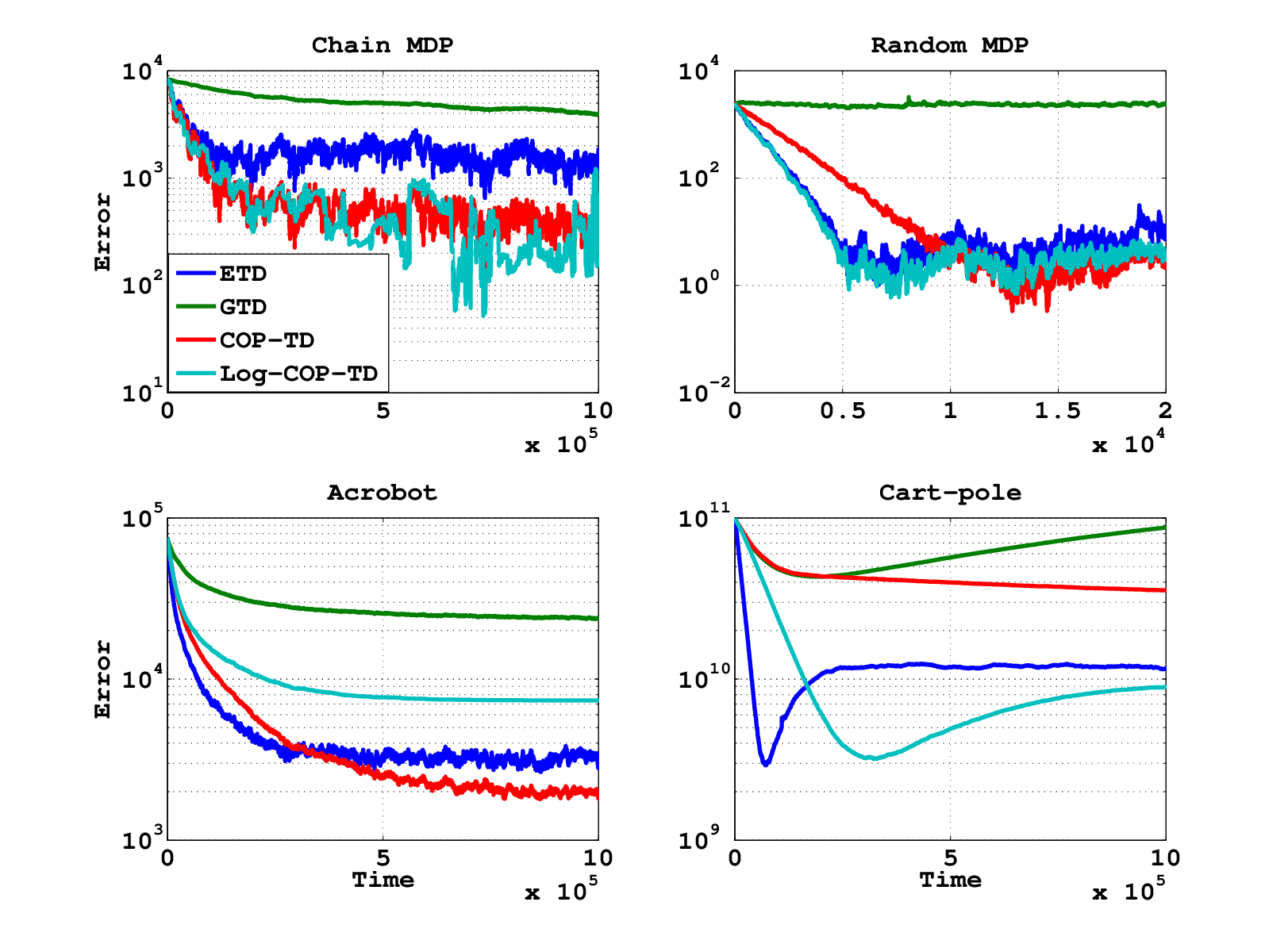
The experiments show that COP-TD($\lambda$, $\beta$) and Log-COP-TD($\lambda$, $\beta$) have comparable performance to ETD($\lambda$, $\beta$) where at least one is better in every setup. The advantage in the new algorithms is especially seen in the chain MDP corresponding to a large discrepancy between the stationary distribution of the behavior and target policy. GTD($\lambda$) is consistently worse on the tested setups, this might be due to the large difference between the chosen behavior and target policies which affects GTD($\lambda$) the most.

Research on off-policy evaluation has flourished in the last decade. While a plethora of algorithms were suggested so far, ETD($\lambda$, $\beta$) by Hallak et al. (2015) has perhaps the simplest formulation and theoretical properties. Unfortunately, ETD($\lambda$, $\beta$) does not converge to the same point achieved by on-line TD when linear function approximation is applied.

We address this issue with COP-TD($\lambda$,$\beta$) and proved it can achieve consistency when used with a correct set of features, or at least allow trading-off some of the bias by adding or removing features. Despite requiring a new set of features and calibrating an additional update function, COP-TD($\lambda$,$\beta$)’s performance does not depend as much on $\beta$ as ETD($\lambda$,$\beta$), and shows promising empirical results.

We offer a connection to the statistical interpretation of TD($\lambda$) that motivates our entire formulation. This interpretation leads to two additional approaches: (a) weight the $\Gamma^{n}_{t}$ using estimated variances instead of $\beta$ exponents and (b) approximating $\log[\rho_{d}]$ instead of $\rho_{d}$; both approaches deserve consideration when facing a real application.

References

- Al-Rawi et al. (2015) Al-Rawi, Hasan AA, Ng, Ming Ann, and Yau, Kok-Lim Alvin. Application of reinforcement learning to routing in distributed wireless networks: a review. Artificial Intelligence Review, 43(3):381–416, 2015.
- Barrett et al. (2013) Barrett, Enda, Howley, Enda, and Duggan, Jim. Applying reinforcement learning towards automating resource allocation and application scalability in the cloud. Concurrency and Computation: Practice and Experience, 25(12):1656–1674, 2013.
- Bertsekas (2012) Bertsekas, D. Dynamic Programming and Optimal Control, Vol II. Athena Scientific, 4th edition, 2012.
- Bertsekas & Tsitsiklis (1996) Bertsekas, D. and Tsitsiklis, J. Neuro-Dynamic Programming. Athena Scientific, 1996.
- Chen & Ye (2011) Chen, Yunmei and Ye, Xiaojing. Projection onto a simplex. arXiv preprint arXiv:1101.6081, 2011.
- Geist & Scherrer (2014) Geist, Matthieu and Scherrer, Bruno. Off-policy learning with eligibility traces: A survey. The Journal of Machine Learning Research, 15(1):289–333, 2014.
- Hachiya et al. (2012) Hachiya, Hirotaka, Sugiyama, Masashi, and Ueda, Naonori. Importance-weighted least-squares probabilistic classifier for covariate shift adaptation with application to human activity recognition. Neurocomputing, 80:93–101, 2012.
- Hallak et al. (2015) Hallak, Assaf, Tamar, Aviv, Munos, Remi, and Mannor, Shie. Generalized emphatic temporal difference learning: Bias-variance analysis. arXiv preprint arXiv:1509.05172, 2015.
- Hochberg et al. (2016) Hochberg, Irit, Feraru, Guy, Kozdoba, Mark, Mannor, Shie, Tennenholtz, Moshe, and Yom-Tov, Elad. Encouraging physical activity in patients with diabetes through automatic personalized feedback via reinforcement learning improves glycemic control. Diabetes care, 39(4):e59–e60, 2016.
- Kober et al. (2013) Kober, Jens, Bagnell, J Andrew, and Peters, Jan. Reinforcement learning in robotics: A survey. The International Journal of Robotics Research, pp. 0278364913495721, 2013.
- Konidaris et al. (2011) Konidaris, George, Niekum, Scott, and Thomas, Philip S. Td-gamma: Re-evaluating complex backups in temporal difference learning. In Advances in Neural Information Processing Systems 24, pp. 2402–2410. Curran Associates, Inc., 2011.
- Kushner & Yin (2003) Kushner, Harold and Yin, G George. Stochastic approximation and recursive algorithms and applications, volume 35. Springer Science & Business Media, 2003.
- Mahmood & Sutton (2015) Mahmood, A Rupam and Sutton, Richard S. Off-policy learning based on weighted importance sampling with linear computational complexity. In Conference on Uncertainty in Artificial Intelligence, 2015.
- Precup et al. (2001) Precup, Doina, Sutton, Richard S, and Dasgupta, Sanjoy. Off-policy temporal-difference learning with function approximation. In ICML, 2001.
- Schuss & Borkar (2009) Schuss, Zeev and Borkar, Vivek S. Stochastic approximation: A dynamical systems viewpoint, 2009.
- Sutton & Barto (1998) Sutton, R. S. and Barto, A. Reinforcement learning: An introduction. Cambridge Univ Press, 1998.
- Sutton et al. (2015) Sutton, R. S., Mahmood, A. R., and White, M. An emphatic approach to the problem of off-policy temporal-difference learning. arXiv:1503.04269, 2015.
- Sutton et al. (2014) Sutton, Rich, Mahmood, Ashique R, Precup, Doina, and Hasselt, Hado V. A new q (lambda) with interim forward view and monte carlo equivalence. In Proceedings of the 31st International Conference on Machine Learning (ICML-14), pp. 568–576, 2014.
- Sutton (1988) Sutton, Richard S. Learning to predict by the methods of temporal differences. Machine learning, 3(1):9–44, 1988.
- Sutton et al. (2009a) Sutton, Richard S, Maei, Hamid R, and Szepesvári, Csaba. A convergent o(n) temporal-difference algorithm for off-policy learning with linear function approximation. In Advances in neural information processing systems, pp. 1609–1616, 2009a.
- Sutton et al. (2009b) Sutton, Richard S, Maei, Hamid Reza, Precup, Doina, Bhatnagar, Shalabh, Silver, David, Szepesvári, Csaba, and Wiewiora, Eric. Fast gradient-descent methods for temporal-difference learning with linear function approximation. In Proceedings of the 26th Annual International Conference on Machine Learning, pp. 993–1000. ACM, 2009b.
- Theocharous & Hallak (2013) Theocharous, Georgios and Hallak, Assaf. Lifetime value marketing using reinforcement learning. RLDM 2013, pp. 19, 2013.
- Theocharous et al. (2015) Theocharous, Georgios, Thomas, Philip S, and Ghavamzadeh, Mohammad. Personalized ad recommendation systems for life-time value optimization with guarantees. In Proceedings of the Twenty-Fourth International Joint Conference on Artificial Intelligence (IJCAI-15), 2015.
- Thomas et al. (2015a) Thomas, Philip, Theocharous, Georgios, and Ghavamzadeh, Mohammad. High confidence policy improvement. In Proceedings of the 32nd International Conference on Machine Learning (ICML-15), pp. 2380–2388, 2015a.
- Thomas et al. (2015b) Thomas, Philip S, Niekum, Scott, Theocharous, Georgios, and Konidaris, George. Policy evaluation using the omega-return. In Advances in Neural Information Processing Systems 28, pp. 334–342. Curran Associates, Inc., 2015b.
- Tsitsiklis & Van Roy (1997) Tsitsiklis, John N and Van Roy, Benjamin. An analysis of temporal-difference learning with function approximation. Automatic Control, IEEE Transactions on, 42(5):674–690, 1997.
- van Hasselt et al. (2014) van Hasselt, Hado, Mahmood, A Rupam, and Sutton, Richard S. Off-policy td () with a true online equivalence. In Proceedings of the 30th Conference on Uncertainty in Artificial Intelligence, Quebec City, Canada, 2014.
- White & White (2016) White, Adam and White, Martha. Investigating practical, linear temporal difference learning. arXiv preprint arXiv:1602.08771, 2016.
- Yu (2015) Yu, H. On convergence of emphatic temporal-difference learning. In COLT, 2015.