Distributions and Statistical Power of Optimal Signal-Detection Methods In Finite Cases

In general there are two types of methods for distribution calculation. The first is to calculate the exact distribution. Recursive methods (e.g., Noe’s recursion[5, 6], Bolshev’s recursion [7, 8], Steck’s recursion [9, 10], Ruben’s recursion [11], etc.) were developed to calculate the distribution of Kolmogorov-Smirnov type statistics under $H_{0}$. In a similar fashion, Barnett and Lin [12] provided a calculation method specifically for HC. Such recursive methods have heavy computation load, with complexity of $O(n^{3})$. Moscovich, Nadler and Spiegelman [13] reduced the computation to $O(n^{2})$. However, all these methods assume the full domain $\mathcal{R}=\{1\leq i\leq n\}$ in the supremum formula of the relevant tests (see the HC statistic in (3) as an example). However, calculation that allows arbitrary $\mathcal{R}$ is important, because many tests improve performance by properly restricting $\mathcal{R}$. For example, a modified version of HC is under $\mathcal{R}=\{1<i\leq n/2,p_{(i)}\geq 1/n\}$. This is because that including too small p-values $p_{(i)}$ could make HC heavy tailed; while including too big p-values may unnecessarily reduces computational efficiency (c.f. [1]). Moreover, these methods did not give statistical power calculation under $H_{1}$ yet.

The second type methods are to approximate the distribution. Kolmogorov-Smirnov type statistics have been proven to converge in law to an extreme-value distribution [15, 16]. However, such convergence is too slow to be accurate for even moderately large $n$ [12]. Recently, Li and Siegmund (LS) [14] developed an asymptotic approximation method. One problems is that this method cannot approximate the whole distribution. Figure 1 shows that the LS calculation (green dotted curves) fails to match the simulation (black solid curves) at small thresholds, whereas our calculation (e.g., the red dashed curves) reveal the whole distributions. Moreover, comparing with our study setting, LS assumes slightly more restriction for the supremum searching domain $\mathcal{R}$, and covers a narrower range of test types. Again, literature studies did not yet provide satisfiable method for deriving the relevant distributions under $H_{1}$ for statistical power calculation.

This paper has two folds of contributions. First, it provides techniques for calculating the distributions of a general family of goodness-of-fit (GOF) tests, which covers the optimal tests described above. We give calculation methods for the exact as well as the approximated distributions, balancing between accuracy and computation burden. The methods allow (A) arbitrary truncation strategies (e.g., $\mathcal{R}$ for HC in (3)), and (B) arbitrary null and alternative hypotheses as long as they are i.i.d. and continuous. With such techniques, p-values and statistical power can be calculated at any testing threshold.

Second, based on analytical calculation we systematically compared the power of the asymptotically optimal tests. Simulations were applied for examing these tests under various $n$ values and signals patterns in practice. We also demonstrated the application of these weak-signal-sensitive tests in a real genome-wide association study (GWAS) for detecting genes associated to the Crohn’s disease (see Figure 2).

In summary, the innovative contribution of this work lies on providing a more mature statistical framework that revolves the problem of calculating distributions for a broader family of GOF tests under both $H_{0}$ and $H_{1}$. Thus, those asymptotically equivalent tests for detecting weak signals can be apply, as well as compared by power, in practical applications. The paper is organized as follows. In section 2 we formulate the problem under a general setup of hypotheses and GOF tests, and brief the essence of our strategy. The analytical results are presented in Section 3 for both exact and approximated calculations. Through simulations Section 4 numerically evidences the calculation accuracy, and provides power comparisons among the asymptotically optimal tests. We show the application of the GOF tests in a real GWAS in Section 5. In Section 6 we discuss relevant theoretical and practical issues. The techniques of relevant proofs and lemmas are given in the Appendix.

We consider the signal detection problem through testing whether there exist “signals” in noisy background. Under the broadly applicable Gaussian Means Model, signals refer to the nonzero means in the normally distributed data values (or statistics) $X_{1},X_{2},...,X_{n}$. A test is said of detecting signals if it successfully concludes the alternative when it is true. A typical setting for the null and the alternative is

$$H_{0}:X_{i}\overset{\text{i.i.d.}}{\sim}N(0,1),\quad H_{1}:X_{i}\overset{\text{i.i.d.}}{\sim}\epsilon N(\mu,1)+(1-\epsilon)N(0,1),$$

(1)

where $\epsilon\in(0,1)$ denotes the expected proportion of signals.

Under the Asymptotic Rare and Weak (ARW) setting, the proportion of signals is $\epsilon_{n}=n^{-\alpha}$, $\alpha\in(1/2,1)$, and the mean is $\mu_{n}=\sqrt{2r\log(n)}$, $r\in(0,1)$. Landmark studies [1, 17, 18] have provided the asymptotic detection boundary in terms of a function curve of the signal strength and sparsity:

$$r=\rho^{\star}(\alpha)=\left\{\begin{array}[]{lr}\alpha-1/2&\quad 1/2<\alpha\leq 3/4\\ (1-\sqrt{1-\alpha})^{2}&\quad 3/4<\alpha<1.\end{array}\right.$$

(2)

When the signals are below the curve, all tests will fail to distinguish $H_{0}$ and $H_{1}$ as $n\rightarrow\infty$. Whenever signals are above the curve, the so-called asymptotically optimal tests are able to make both the type I and the type II error rates converge to zero. A particular optimal test is the Higher Criticism (HC) test [19, 1]:

$$HC_{n,\mathcal{R}}=\sup_{\mathcal{R}}\sqrt{n}\frac{i/n-p_{(i)}}{\sqrt{p_{(i)}(1-p_{(i)})}},$$

(3)

where $p_{(1)}\leq...\leq p_{(n)}$ are the order statistics of $p_{i}=2(1-F_{0}(|X_{i}|)),i=1,...,n$, the two-sided p-values of $X_{i}$. The supremum domain $\mathcal{R}$ regards to the p-value magnitude, or the index $i$, or both. Note that in literature HC formula could also be written as (e.g., [20, 12] )

$$HC=\sup_{t\in\mathcal{R}^{*}}\frac{\sum_{i}\{X_{i}>t\}-2n\bar{\Phi}(t)}{\sqrt{2n\bar{\Phi}(t)\Phi(t)}}.$$

(4)

Because the formula is monotone, the supremum domain $\mathcal{R}$ on $p_{(i)}$ is equivalent to the supremum domain $\mathcal{R}^{*}$ on $t$.

Following that, a variety of modified Higher Criticism (HC), the Berk-Jones (B-J) type tests, a spectrum of $\phi$-divergence type tests, etc. were studied and proven asymptotically optimal [1, 2, 3, 4]. In this paper, we provide calculation for the p-value and statistical power for relevant tests under finite $n$.

In this paper, we consider arbitrary i.i.d. and continuous null and alternative hypotheses:

$$H_{0}:X_{i}\overset{\text{i.i.d.}}{\sim}F_{0},\quad H_{a}:X_{i}\overset{\text{i.i.d.}}{\sim}F_{1},i=1,...,n.$$

(5)

We consider the goodness-of-fit (GOF) tests that evidence the distinction between the data and any given null distribution. Consider either one-sided p-values $p_{i}=1-F_{0}(X_{i})$ or two-sided p-values $p_{i}=2(1-F_{0}(|X_{i}|))$. When $F_{0}$ is continuous, the null hypothesis is equivalent to

$\displaystyle H_{0}:p_{i}\overset{\text{i.i.d.}}{\sim}\text{Uniform}(0,1),i=1,...,n.$

The typical idea of GOF is that if any $X_{i}$ do not follow $F_{0}$, its $p_{(i)}$ shall distinct from it expectation, which is roughly $i/n$. Following this idea we consider a general family of tests,

$$S_{n,\mathcal{R}}=\sup_{\mathcal{R}}f(\frac{i}{n},p_{(i)}),$$

(6)

where the supremum domain

$$\mathcal{R}=\{i:k_{0}\leq i\leq k_{1}\}\bigcap\{p_{(i)}:\alpha_{0}\leq p_{(i)}\leq\alpha_{1}\}$$

(7)

for given $k_{0}\leq k_{1}\in\{1,...,n\}$ and $\alpha_{0}\leq\alpha_{1}\in[0,1]$. We assume that for fixed $x=i/n$ the function $f(x,y)$ is monotonically decreasing in $y=p_{(i)}$, so that the smaller the input p-values, the larger the statistic and the stronger the evidence against $H_{0}$.

This GOF family contains lots of test statistics widely applicable to practice. For example, the simple one-sided Kolmogorov-Smirnov test statistic (c.f. [21], page 447, denoted $KS^{+}$ here) is a classic GOF test, which directly measures the difference between $p_{(i)}$ and $i/n$. That is, the $f$ function is defined by

$$f_{KS^{+}}(x,y)=x-y.$$

(8)

To improve the test, the difference between $p_{(i)}$ and $i/n$ should be scaled with regard to $p_{(i)}$ or $i/n$. This is because smaller $p_{(i)}$ values are more important to evidence agains $H_{0}$. Such scaled KS tests are related to the Higher Criticism (HC) statistics proposed in 2004 and 2008 [1, 2], respectively, where the $f$ functions are defined as

$$\begin{array}[]{ll}f_{HC^{2004}}(x,y)&=\sqrt{n}\displaystyle\frac{x-y}{\sqrt{y(1-y)}}\text{; }\\ f_{HC^{2008}}(x,y)&=\sqrt{n}\displaystyle\frac{x-y}{\sqrt{x(1-x)}}.\end{array}$$

(9)

Jager and Wellner introduced a collection of $\phi$-divergence statistics [4], which are also based on the supremum of functions:

$$\begin{array}[]{ll}f^{\phi}_{s}(x,y)&=\displaystyle\frac{1}{s(1-s)}(1-x^{s}y^{1-s}-(1-x)^{s}(1-y)^{1-s})\text{, }s\neq 0,1,\\ f^{\phi}_{1}(x,y)&=x\log(\displaystyle\frac{x}{y})+(1-x)\log(\frac{1-x}{1-y}),\\ f^{\phi}_{0}(x,y)&=y\log(\displaystyle\frac{y}{x})+(1-y)\log(\frac{1-y}{1-x}).\end{array}$$

(10)

For certain $s$ (e.g., $s=2$ or $-1$) these statistics are two-sided in the sense that switching the values of $x=i/n$ and $y=p_{(i)}$ gives the same statistic. However, this property is not appropriate in the scenario of signal detection. It is the relationship $p_{(i)}<i/n$, instead of the opposite, indicates signals. Thus for signal detection purpose, one-sided test is more reasonable and more powerful, as is the same idea for defining KS and HC. Thus, here we consider the one-sided version of $\phi$-divergence statistics, which can be achieved by a simple adjustment of the $f$ function to be, for example,

$$f_{s}(x,y)=\left\{\begin{array}[]{lr}\sqrt{2nf^{\phi}_{s}(x,y)}&\quad y\leq x,\\ -\sqrt{2nf^{\phi}_{s}(x,y)}&\quad y>x.\end{array}\right.$$

(11)

Now for all $s$, $f_{s}(x,y)$ is guaranteed decreasing in y. Such one-sided $\phi$-divergence statistics cover HC exactly: $f_{2}=f_{HC^{2004}}$ and $f_{-1}=f_{HC^{2008}}$. Also, $s=1$ and $0$ correspond to the Berk-Jones statistic [22, 1, 14] and the reverse Berk-Jones statistic [22], respectively. Note that the input p-values themselves could be two-sided in order to accommodate the consideration of signal directionality in practical problems.

In the following we first introduce the essential idea of the calculation. Under various settings and assumptions, detailed strategies for obtaining the exact and approximated distributions will be described in Section 3.

For any given continuous CDFs in (5), we define a monotone transformation function in $(0,1)$:

$$D(x)=\left\{\begin{array}[]{l l}x&\quad\text{under $H_{0}:F_{0}$},\\ 1-F_{1}(F_{0}^{-1}(1-x))&\quad\text{under $H_{1}:F_{1}\neq F_{0}$}.\end{array}\right.$$

(12)

Note that for any p-value $p_{i}$, we have $D(p_{i})\sim Uniform(0,1)$ under either $H_{0}$ or $H_{1}$.

Consider the function $f(x,y)$ of any statistic $S_{n,\mathcal{R}}$ in (6), for each fixed $x$ define its inverse function

$$g(x,\cdot)=f^{-1}(x,\cdot).$$

(13)

For example, for the HC statistics defined (9), the $g$ functions are

$$\begin{array}[]{ll}g_{HC^{2004}}(x,b)=\frac{1}{1+b^{2}/n}[x+\frac{b^{2}/n-(b/\sqrt{n})\sqrt{b^{2}/n+4x(1-x)}}{2}]\text{; }\\ g_{HC^{2008}}(x,b)=x-(b/\sqrt{n})\sqrt{x(1-x)}.\end{array}$$

(14)

In general if the closed form of $g(x,\cdot)$ is not available, it can always be found numerically, since $f(x,y)$ is strictly decreasing in $y$.

Now under either $H_{0}$ or $H_{1}$, the CDF function of $S_{n,\mathcal{R}}$ is

$$\begin{array}[]{l l}P(S_{n}\leq b)&=P(\displaystyle\sup_{\mathcal{R}}f(\frac{i}{n},p_{(i)})\leq b)\\ &=P(\displaystyle\bigcap_{\mathcal{R}}\{p_{(i)}>g(\frac{i}{n},b)\})\\ &=P\{D(p_{(i)})>D(g(\frac{i}{n},b)),\text{all }i\text{ and }p_{(i)}\text{ in }\mathcal{R}\}.\end{array}$$

(15)

The key idea is that under either $H_{0}$ or $H_{1}$, $U_{(i)}:=D(p_{(i)})$ is the $i^{th}$ order statistic of Uniform(0, 1), and the joint distribution of $U_{(i)}$, $i=k_{0},....,k_{1}$, can be studies one way or another for getting the final probability.

To simplify the presentation, we list below the notations to be referred later on.

• (N1)

  $u_{k}:=D(g(\frac{k}{n},b)\vee\alpha_{0})$, following the definitions in (12)–(15), and a potential constant $\alpha_{0}\geq 0$ in (7).

• (N2)

  $\bar{F}_{B(\alpha,\beta)}(x)$ denotes the survival function of $Beta(\alpha,\beta)$ distribution.

• (N3)

  $F_{\Gamma(\alpha)}(x)$ and $\bar{F}_{\Gamma(\alpha)}(x)$ denote the CDF and survival function of $Gamma(\alpha,1)$ distribution, respectively, where the shape parameter is $\alpha$, the scale parameter is 1.

• (N4)

  Based on the notation (N3) define

  $$h_{k}(x):=xF_{\Gamma(k-1)}(kx)-F_{\Gamma(k)}(kx).$$

• (N5)

  $f_{P(\lambda)}(x)$ denotes the probability mass function of $Poisson(\lambda)$ distribution.

The first theorem provides the exact calculation for the distribution of GOF in (6), where the supremum domain $\mathcal{R}$ involves truncation of the index $i$. For example, the initial HC was defined with $\mathcal{R}=\{1\leq i\leq n/2\}$ [1].

Another type of truncation is based on the value of $p_{(i)}$. In the case of HC under the null of $N(0,1)$, this truncation is equivalent to the truncation on $t$ in (4). The following theorem gives the exact calculation for the general GOF tests in (6) with such truncations.

The most general $\mathcal{R}$ is in (7), which defines the truncation for both the index and the p-values. The following theorem provides the calculation for exact distribution under this general setup, for which no literature has provided solution before.

The study setting in Li and Siegmund [14] is a special case of the general truncation with $\alpha_{1}=1$. For example, the “modified HC” is to take $\mathcal{R}=\{1<i\leq n/2,p_{(i)}\geq 1/n\}$[1]. Li and Siegmund’s calculation provided an approximation for the modified HC under $H_{0}$. As shown in Figure 1, the approximation does not give the whole distribution. For this setting, the corollary below gives the exact distribution for the general GOF in (6) under both $H_{0}$ and $H_{1}$.

To sum up, Theorem 3.3 covers Theorem 3.1 by fixing $i=1,j=n+1$ (so that $c_{ij}=0$) and $\alpha_{0}=0,\alpha_{1}=1$. It covers Theorem 3.2 by letting $k_{0}=1,k_{1}=n$, and covers Corollary 1 by fixing $j=n+1$ and $\alpha_{1}=1$.

Regarding the computational complexity, the calculation given by Theorem 3.1 is equivalent to solving an upper triangular linear systems using backward substitution, which is $O(n^{2})$, an improvement from $O(n^{3})$ required by other exact distribution calculations [5, 6, 12]. More importantly, our method can handle a more general family of GOFs defined in (6) with a more flexible supremum domain $\mathcal{R}$. When $\mathcal{R}$ is more complicated, Corollary 1 is still $O(n^{2})$ because the inner loop $a_{k}$ is not dependent on $i$. Theorem 3.2 and Theorem 3.3 are $O(n^{3})$.

In this section, we provide several calculation methods to approximate the distributions of the GOF family. Under more restricted conditions, computation load could be significantly reduced. For simplicity we provide results here for the supremum domain $\mathcal{R}=\{k_{0}\leq i\leq k_{1}\}$. More general results for $\mathcal{R}$ in (7) can be obtained by following the similar idea of the calculation in Theorem 3.3.

The theorem below gives an approximated calculation based on a joint Gamma distribution.

To further reduce the computation, we can also deduce a one-step formula under stronger assumptions. In particular, if $D(g(\frac{k}{n},b))$ is a linear function of $k$, we can provide a closed-form formula for the distribution that gives the same accuracy as the above theorem.

One example that satisfies the linearity of $D(g(\frac{k}{n},b))$ is the simple Kolmogorov-Smirnov ($KS^{+}$) test in (8) under $H_{0}$, where $a=-(n+1)b$ and $\lambda=\frac{n+1}{n}$. In this case, based on the above theorem we have the following corollary

The requirement of linear $D(g(\frac{k}{n},b))$ in Theorem 3.5 is stringent. However, if $D(g(\frac{k}{n},b))$ is close to linear, we can still further simplify the calculation of Theorem 3.4. As one example, Theorem 3.6 below provides such a calculation formula for GOF and the conditions on $D(g(\frac{k}{n},b))$. The strategy for proving this theorem largely follows the idea in Li and Siegmund [14]. The key difference is that, instead of using the beta distribution in Li and Siegmund, we use the gamma distribution, which has a simpler density function for addressing a wider family of the GOF tests. See Appendix for details.

Such a close-to-linear property of $D(g(\frac{k}{n},b))$ can be satisfied by $HC^{2004}$ under $H_{0}$. In this case, $D(g(\frac{k}{n},b))=g(x,b)$ is given in (14), and the conditions can be satisfied when $b$ is in the order of $O(\sqrt{n})$. Thus, we can get a computation-easy formula.

The above formula is different from that given in Li and Sigmund [14]. However, for the HC under $H_{0}$, both formulas require the threshold $b=O(\sqrt{n})$. Thus, both methods do not get the whole distribution. Furthermore, the accuracy depends on the linear approximation of the $D(g(\frac{k}{n},b))$ function, which could be far from the truth under general $H_{1}$. Thus this type of calculation may not be very attractive for calculation statistical power. Meanwhile, numeric results in Section 4 show that both methods are accurate for calculating small p-values under relatively large threshold $b$.

Under $H_{0}:X_{i}\overset{\text{i.i.d.}}{\sim}N(0,1),i=1,...,n$. Figure 3 shows the right-tail probability of HC over the threshold $b$. Comparing with simulation (black solid curves), the exact calculation by Theorem 3.1 (cyan dashed curves) has a perfect match. The approximation by Theorem 3.4 is accurate over the whole distribution when $n$ is fairly big. The closed-formula calculation methods by Li and Siegmund [14] (blue dotted curves) and by Corollary 3 (green dashed curves) do not fit the whole distribution curve, but both can provide good approximation for calculation small p-values at large threshold.

For distribution calculation under the alternative, we considered the null of i.i.d. $N(0,1)$ (on which the input p-values are based) and the alternatives:

		$\displaystyle H_{1}:X_{i}\overset{\text{i.i.d.}}{\sim}(1-\epsilon)N(0,1)+\epsilon N(1,1),\text{ or}$
		$\displaystyle H_{1}:X_{i}\overset{\text{i.i.d.}}{\sim}(1-\epsilon)N(0,1)+\epsilon t_{\nu}.$

Figure 4 shows the right-tail probability of HC under the normal mixture alternative with $\mu=1$, $\epsilon=0.1$ (row 1), or under the Student’s $t$ distribution with degrees of freedom $\nu=5$ (row 2). In both cases the distribution curves by exact calculation (Theorem 3.1, cyan dashed curves) and by approximation (Theorem 3.4, red dot-dashed) are close to simulation (black solid curves). As expected, the approximation is more accurate for larger $n$.

Besides the normal distributions, Theorems 3.1 – 3.4 can handle any given continuous $F_{0}$ and $F_{1}$. Here we test on four settings studied in the initial paper of HC [1]. The first setting regards a Chi-squared model:

$\displaystyle H_{0}:X_{i}\overset{\text{i.i.d.}}{\sim}\chi^{2}_{\nu}(0),\quad\text{ vs. }\quad H_{1}:X_{i}\overset{\text{i.i.d.}}{\sim}(1-\epsilon)\chi^{2}_{\nu}(0)+\epsilon\chi^{2}_{\nu}(\delta).$

where $\nu$ is the degree of freedom, $\delta$ is the non-centrality parameter. The second setting is a Student’s t mixture model:

$\displaystyle H_{0}:X_{i}\overset{\text{i.i.d.}}{\sim}t_{\nu}(0),\quad\text{ vs. }\quad H_{1}:X_{i}\overset{\text{i.i.d.}}{\sim}(1-\epsilon)t_{\nu}(0)+\epsilon t_{\nu}(\delta).$

The third setting is a chi-squared-exponential mixture model,

$\displaystyle H_{0}:X_{i}\overset{\text{i.i.d.}}{\sim}\exp(\nu),\quad\text{ vs. }\quad H_{1}:X_{i}\overset{\text{i.i.d.}}{\sim}(1-\epsilon)\exp(\nu)+\epsilon\chi^{2}_{\nu}(\delta).$

The fourth setting concerns a generalized normal distribution (also known as power exponential distribution) model,

$\displaystyle H_{0}:X_{i}\overset{\text{i.i.d.}}{\sim}GN_{p}(0,\sigma),\quad\text{ vs. }\quad H_{1}:X_{i}\overset{\text{i.i.d.}}{\sim}(1-\epsilon)GN_{p}(0,\sigma)+\epsilon GN_{p}(\mu,\sigma),$

where the probability density function of $GN_{p}(\mu,\sigma)$ is

$\displaystyle\frac{1}{C_{p}}\exp(-\frac{|x-\mu|^{p}}{p\sigma^{p}}),\quad C_{p}=2p^{1/p}\Gamma(1+1/p)\sigma.$

Notice that $GN_{1}(\mu,\sigma)$ is the Laplace distribution and $GN_{2}(\mu,\sigma)$ is $N(\mu,\sigma^{2})$. Each row of Figure 5 illustrates the alternative distribution of HC under each of the four settings for $n=10$ (left column) and $100$ (right column). Again the distribution calculation is fairly accurate in all cases.

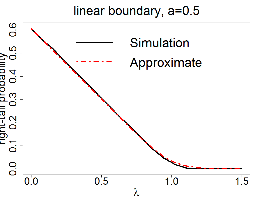
For the closed-form calculation formula given by Theorem 3.5, the boundary is assumed linear: $D(g(\frac{i}{n},b))=a+\lambda k\geq 0$ in (15). One example is the $KS^{+}$ in (8) under $H_{0}$. Figure 6 demonstrates the accuracy of the calculation based on either fixed slope $\lambda=0.5$ or fixed intercept $a=0.5$. Here $k_{0}=1$, $k_{1}=n=50$. As the boundary $a+\lambda k$ increases, the probabilities from both calculation and simulation decrease and well-matched as expected.

All $\phi$-divergence statistics with $s\in[-1,2]$ possess the same asymptotic optimality property for detecting weak and sparse signals [4]. It is of interest to know the performance of such statistics under finite $n$. Here we study $s=2,1,0,-1$, which correspond to $HC^{2004}$, the Berk-Jones statistic, the reverse Berk-Jones statistic, and $HC^{2008}$, respectively.

To show the calculation accuracy, we calculated (by Theorem 3.1) the critical values at the significance levels of $10\%$, $5\%$ and $1\%$. Then at these critical values we got the empirical type I error rates through simulation (10,000 repetitions). Table 1 presents the thresholds by calculation and the correspondingly empirical type I error rates. The closeness of these empirical and nominal type I error rates evidences that the calculation for these tests is accurate.

Now through the calculation based on Theorem 3.1, we systematically compared the power of these tests under

$\displaystyle H_{0}:X_{i}\overset{\text{i.i.d.}}{\sim}N(0,1),\quad\text{ vs. }\quad H_{1}:X_{i}\overset{\text{i.i.d.}}{\sim}(1-\epsilon)N(0,1)+\epsilon N(\mu,1).$

With the type I error rate controlled at 5%, Figure 7 provides the statistical power at various $\mu$, $n$ and $\epsilon$. There are a few interesting observations. First, $HC^{2004}$ performs well when signals are sparse. However, it seems more relevant to the average number of signals, i.e., $\epsilon n$, rather than the proportion $\epsilon$ itself. For example, at fixed $\epsilon n=5$ (panels in the first column), $HC^{2004}$ is always the best, while at fixed $\epsilon=0.05$ (panels in the diagonal), $HC^{2004}$ becomes worse when $n$ increases. Second, Smaller $s$ parameter ($s=-1$ for $HC^{2008}$ and $s=0$ for the reverse Berk-Jones) gives better power for denser signals. However, when signals are sparse, they are less powerful because these statistics are insensitive to small p-values as they are weighted by $i/n$ rather than $p_{(i)}$. Third, Berk-Jones statistic has a more robust performance over various $\mu$, $n$ and $\epsilon$, which is consistent with the finding of Li and Siegmund [14].

Moreover, it is interesting to see the performance of these methods along the asymptotic detection boundary. This is because the optimal tests are most valuable for detecting subtle signals around the detection boundary, for which sub-optimal tests will have asymptotically zero power. Here we consider the ARW setting with the detection boundary given in (2). Figure 8 shows the power (calculated by Theorem 3.1) of the four methods over the sparsity parameter $\alpha\in(1/2,1)$ and $r$ calculated accordingly. It shows that the power curves of $HC^{2004}$ and B-J have the similar pattern, while the performance of $HC^{2008}$ and reverse B-J are alike. In the less sparse case with $\alpha\in(1/2,3/4)$, B-J is preferred; in the sparser case with $\alpha\in(3/4,1)$, $HC^{2004}$ outperforms the others.

Last but not least, the supremum domain $\mathcal{R}$ in (6) is quite relevant in constructing the test statistic. Here we compare $HC^{2004}$ under $\mathcal{R}=\{1\leq i\leq n/2\}$ with the modified HC under $\mathcal{R}=\{1<i\leq n/2,p_{(i)}\geq 1/n\}$. Figure 9 shows that the MHC performs poorly when the number of signals is small, whereas it improves the performance when the number of signals increases. When signals are sparse, MHC is less powerful because it tends to exclude signals by considering only those p-values bigger than $1/n$, the latter is a fairly large value when $n$ is small. Thus, in practice when $n$ is not too big, there may be no need to truncate p-values by $1/n$.

References

- [1] D. Donoho and J. Jin, “Higher criticism for detecting sparse heterogeneous mixtures,” The Annals of Statistics, vol. 32, no. 3, pp. 962–994, 2004.
- [2] D. Donoho and J. Jin, “Higher criticism thresholding: Optimal feature selection when useful features are rare and weak,” Proceedings of the National Academy of Sciences of the United States of America, vol. 105, pp. 14790–14795, Sep 30 2008.
- [3] D. Donoho and J. Jin, “Higher criticism for large-scale inference: especially for rare and weak effects,” Statistical Science, vol. 30, no. 1, pp. 1–25 DOI: 10.1214/14–STS506, 2015.
- [4] L. Jager and J. A. Wellner, “Goodness-of-fit tests via phi-divergences,” The Annals of Statistics, pp. 2018–2053, 2007.
- [5] M. Noé, “The calculation of distributions of two-sided kolmogorov-smirnov type statistics,” The Annals of Mathematical Statistics, pp. 58–64, 1972.
- [6] M. Noé and G. Vandewiele, “The calculation of distributions of kolmogorov-smirnov type statistics including a table of significance points for a particular case,” The Annals of Mathematical Statistics, vol. 39, no. 1, pp. 233–241, 1968.
- [7] V. Kotel’Nikova and E. Chmaladze, “On computing the probability of an empirical process not crossing a curvilinear boundary,” Theory of Probability & Its Applications, vol. 27, no. 3, pp. 640–648, 1983.
- [8] G. R. Shorack and J. A. Wellner, Empirical processes with applications to statistics, vol. 59. SIAM, 2009.
- [9] G. Steck, “The smirnov two sample tests as rank tests,” The Annals of Mathematical Statistics, pp. 1449–1466, 1969.
- [10] M. Breth, “On a recurrence of steck,” Journal of Applied Probability, pp. 823–825, 1976.
- [11] H. Ruben, “On the evaluation of steck’s determinant for rectangle probabilities of uniform order statistics,” Communications in Statistics-Theory and Methods, vol. 5, no. 6, pp. 535–543, 1976.
- [12] I. J. Barnett and X. Lin, “Analytical p-value calculation for the higher criticism test in finite-d problems,” Biometrika, vol. 101, no. 4, pp. 964–970, 2014.
- [13] A. Moscovich, B. Nadler, C. Spiegelman, et al., “On the exact berk-jones statistics and their -value calculation,” Electronic Journal of Statistics, vol. 10, no. 2, pp. 2329–2354, 2016.
- [14] J. Li and D. Siegmund, “Higher criticism: p-values and criticism,” Annals of Statistics, vol. 43, no. 3, pp. 1323–1350, 2015.
- [15] F. Eicker, “The asymptotic distribution of the suprema of the standardized empirical processes,” The Annals of Statistics, pp. 116–138, 1979.
- [16] D. Jaeschke, “The asymptotic distribution of the supremum of the standardized empirical distribution function on subintervals,” The Annals of Statistics, vol. 7, no. 1, pp. 108–115, 1979.
- [17] Y. I. Ingster, “Some problems of hypothesis testing leading to infinitely divisible distributions,” Mathematical Methods of Statistics, vol. 6, no. 1, pp. 47–69, 1997.
- [18] Y. I. Ingster, “Minimax detection of a signal for -balls,” Mathematical Methods of Statistics, vol. 7, no. 4, pp. 401–428, 1998.
- [19] J. Tukey, “The higher criticism.” Course Notes, Statistics 411, Princeton University., 1976.
- [20] E. Arias-Castro, E. J. Candès, and Y. Plan, “Global testing under sparse alternatives: Anova, multiple comparisons and the higher criticism,” The Annals of Statistics, vol. 39, no. 5, pp. 2533–2556, 2011.
- [21] J. Shao, Mathematical Statistics. Springer Verlag, 2010.
- [22] R. H. Berk and D. H. Jones, “Goodness-of-fit test statistics that dominate the kolmogorov statistics,” Probability Theory and Related Fields, vol. 47, no. 1, pp. 47–59, 1979.
- [23] D. B. Goldstein, “Common genetic variation and human traits,” New England Journal of Medicine, vol. 360, no. 17, pp. 1696–1698, 2009.
- [24] A. L. Price, N. J. Patterson, R. M. Plenge, M. E. Weinblatt, N. A. Shadick, and D. Reich, “Principal components analysis corrects for stratification in genome-wide association studies,” Nature genetics, vol. 38, no. 8, pp. 904–909, 2006.
- [25] P. McCullagh and J. A. Nelder, Generalized linear models, vol. 37. CRC press, 1989.
- [26] D. J. Schaid, C. M. Rowland, D. E. Tines, R. M. Jacobson, and G. A. Poland, “Score tests for association between traits and haplotypes when linkage phase is ambiguous,” The American Journal of Human Genetics, vol. 70, no. 2, pp. 425–434, 2002.
- [27] R. Duerr, K. Taylor, S. Brant, J. Rioux, M. Silverberg, M. Daly, A. Steinhart, C. Abraham, M. Regueiro, A. Griffiths, et al., “A genome–wide association study identifies il23r as an inflammatory bowel disease gene,” Science Signalling, vol. 314, no. 5804, p. 1461, 2006.
- [28] J.-P. Hugot, M. Chamaillard, H. Zouali, S. Lesage, J.-P. Cézard, J. Belaiche, S. Almer, C. Tysk, C. A. O’Morain, M. Gassull, et al., “Association of nod2 leucine-rich repeat variants with susceptibility to crohn’s disease,” Nature, vol. 411, no. 6837, pp. 599–603, 2001.
- [29] Y. Ogura, D. K. Bonen, N. Inohara, D. L. Nicolae, F. F. Chen, R. Ramos, H. Britton, T. Moran, R. Karaliuskas, R. H. Duerr, et al., “A frameshift mutation in nod2 associated with susceptibility to crohn’s disease,” Nature, vol. 411, no. 6837, pp. 603–606, 2001.
- [30] D. Maglott, J. Ostell, K. D. Pruitt, and T. Tatusova, “Entrez gene: gene-centered information at ncbi,” Nucleic acids research, vol. 39, no. suppl 1, pp. D52–D57, 2011.
- [31] P. Chamouard, Z. Richert, N. Meyer, G. Rahmi, and R. Baumann, “Diagnostic value of c-reactive protein for predicting activity level of crohns disease,” Clinical Gastroenterology and Hepatology, vol. 4, no. 7, pp. 882–887, 2006.
- [32] G. Trikudanathan, P. G. Venkatesh, and U. Navaneethan, “Diagnosis and therapeutic management of extra-intestinal manifestations of inflammatory bowel disease,” Drugs, vol. 72, no. 18, pp. 2333–2349, 2012.
- [33] W. D. James, T. Berger, and D. Elston, Andrew’s diseases of the skin: clinical dermatology. Elsevier Health Sciences, 2011.
- [34] S. Yuvaraj, S. H. Al-Lahham, R. Somasundaram, P. A. Figaroa, M. P. Peppelenbosch, and N. A. Bos, “E. coli-produced bmp-2 as a chemopreventive strategy for colon cancer: a proof-of-concept study,” Gastroenterology research and practice, vol. 2012, 2012.
- [35] M. L. Slattery, A. Lundgreen, J. S. Herrick, S. Kadlubar, B. J. Caan, J. D. Potter, and R. K. Wolff, “Genetic variation in bone morphogenetic protein and colon and rectal cancer,” International Journal of Cancer, vol. 130, no. 3, pp. 653–664, 2012.
- [36] H. David and H. Nagaraja, “Order statistics,” 2003.
- [37] A. M. Mathai and P. G. Moschopoulos, “On a multivariate gamma,” Journal of Multivariate Analysis, vol. 39, no. 1, pp. 135–153, 1991.