Detecting causal associations in large nonlinear time series datasets
Abstract
Identifying causal relationships from observational time series data is a key problem in disciplines such as climate science or neuroscience, where experiments are often not possible. Data-driven causal inference is challenging since datasets are often high-dimensional and nonlinear with limited sample sizes. Here we introduce a novel method that flexibly combines linear or nonlinear conditional independence tests with a causal discovery algorithm that allows to reconstruct causal networks from large-scale time series datasets. We validate the method on a well-established climatic teleconnection connecting the tropical Pacific with extra-tropical temperatures and using large-scale synthetic datasets mimicking the typical properties of real data. The experiments demonstrate that our method outperforms alternative techniques in detection power from small to large-scale datasets and opens up entirely new possibilities to discover causal networks from time series across a range of research fields.
Introduction
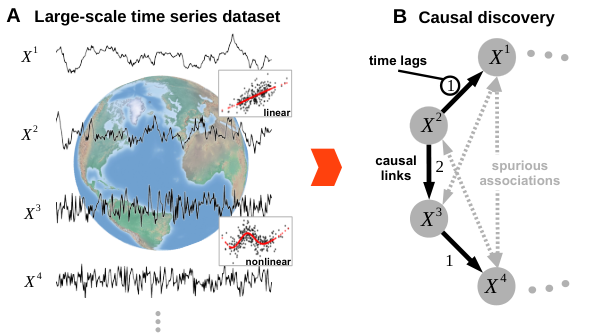
How do major climate modes such as the El Niño Southern Oscillation (ENSO) or the North Atlantic Oscillation couple to remote regions via global teleconnections? Through which pathways do different brain regions interact? Identifying causal association networks of multiple variables is a key challenge in the analysis of such complex dynamical systems, especially since here interventional real experiments, the gold standard of scientific discovery, are often expensive, unethical, or practically impossible. In climate research, model simulations can help to discover causal mechanisms, but confidence in the results is limited due to the realism of the modeled physical processes, which is often not given [1]. Therefore, there is an urgent need to reconstruct causal association networks from observational time series which has become more attractive since recent decades have seen an explosion in the availability of computational resources, cheap data storage, and automated observational data capture of many forms (satellite data, station-based observations, field site measurements [2]), as well as climate model output [1].
In a typical scenario in climate science a researcher has an hypothesis on the causal influence between two climatological processes given observed time series data. For example, she may be interested in the influence of ENSO on temperatures over North America. Suppose the time series show a clear correlation, suggesting a relationship between the two processes. In order to exclude other possible hypotheses that may explain such a correlation, she will then include other relevant variables. In the highly interconnected climate system there are many possible drivers she could test, quickly leading to high-dimensional causal discovery problems.
The goal in time series causal discovery from complex dynamical systems is to reliably reconstruct causal links including their time lags since, e.g., climatic teleconnections typically take days to months. The challenge lies in typically high-dimensional and strongly interdependent datasets comprising dozens to hundreds of variables where correlations in some cases arise due to direct causal effects, but also due to a plethora of other reasons, including autocorrelation within each time series, indirect links, and common drivers (Fig. 1). Ideally, a causal discovery method detects as many true causal relationships as possible (high detection power) and controls the number of false positives (incorrect link detections).
A major current approach in Earth data analysis[3, 4, 5, 6], but also in neuroscience[7, 8], is to test time-lagged causal associations using autoregressive models in the framework of Granger causality [9, 10]. If implemented using standard regression techniques, the high-dimensionality of typical datasets leads to very low detection power (“curse of dimensionality”) since sample sizes are often only on the order of few hundreds (e.g., for a monthly time resolution with 30 years of satellite data). This shortcoming leads to a dilemma that has limited applications of Granger causality mostly to bivariate analyses that cannot, however, account for indirect links and common drivers.
There are methods that can cope with high-dimensionality such as regularized regression techniques [11, 12], but mainly in the context of prediction and not causal discovery where assessing the significance of causal links is more important. An exception is Lasso regression[11] which also allows to discover active variables. Another approach with some recent applications in climate research[13, 14, 15] are algorithms aimed specifically at causal discovery [16, 17, 18], which remove redundant or irrelevant variables utilizing iterative independence and conditional independence testing. However, both regularized regression and recent implementations of causal discovery algorithms do not deal well with the strong interdependencies due to the spatio-temporal nature of the variables as we show here. In particular, controlling false positives at a desired level is difficult for such methods [19, 20, 21], and becomes even more challenging for nonlinear estimators. In summary, these problems lead to brittle causal network reconstructions and a more reliable methodology is required.
We present a causal discovery method suitable for moderately large time series datasets on the order of tens to hundreds of variables featuring linear as well as nonlinear, time-delayed dependencies given sample sizes of a few hundreds or more. Through analytical results and extensive numerical experiments we demonstrate that the proposed method has advantages over the current state-of-the-art approaches in dealing with high-dimensional interdependent time series datasets yielding reliable false positive control and higher detection power without significantly increasing computational demand. Our approach enables causal analyses among much more variables opening up new possibilities to more credibly reconstruct causal networks from time series in Earth system science, neuroscience, and many other fields.
Causal discovery

Motivating example from climate science
In the following, we illustrate the causal discovery problem on a well-known tropical-extratropical long-range teleconnection. We work out two main factors which lead the common autoregressive modeling approach to have low detection power: reduced effect size due to conditioning on irrelevant variables and high-dimensionality.
Given a finite time series sample, every causal discovery method has to balance the trade-off between too many false positives (incorrect link detections) and too few true positives (correct link detections). A causality method ideally controls false positives at a pre-defined significance level (typically 5%) and maximizes detection power. The power of a method to detect a causal link depends on the available sample size, the significance level, the dimensionality of the problem (e.g., the number of coefficients in an autoregressive model), and effect size, which is the magnitude of the effect as measured by the test measure (e.g., the partial correlation coefficient). Since sample size and significance level are usually fixed in the present context, a method’s power can only be improved by reducing the dimensionality or increasing the effect size (or both).
Consider a typical causal discovery scenario in climate research (Fig. 2). We wish to test whether the observational data supports the hypothesis that tropical Pacific surface temperatures, as represented by the monthly Nino 3.4 index (see map and region in Supplementary Fig. S2, further referred to as Nino) [22, 24], causally affect extratropical land air temperatures over British Columbia (BCT) 1979–2017 ( months). We chose this example since it is well-established and physically understood that atmospheric wave trains induced by increased sea-surface temperatures over the tropical Pacific can affect North American temperatures, but not the other way around[25, 26, 6]. Thus, the ground truth here is on the (intra-)seasonal time scale allowing us to validate causality methods.
We start with a time-lagged correlation analysis and find that both variables are correlated in both directions, that is, for both positive and negative lags (Fig. 2A, see Supplementary Fig. S2 for lag functions), suggesting also an influence from BCT on Nino. The correlation has an effect size of () at a lag of two months. In the networks in Fig. 2 the link colors denote effect sizes (grey links are spurious) and the node colors denote the autocorrelation strength.
Clearly, lagged correlation cannot be used to infer causal directionality, and not even the correct time lag of a coupling [14]. Hence, we now move to causal methods. To test , the most straightforward approach then is to fit a linear autoregressive model of BCT on past lags of itself as well as Nino and test whether and which past coefficients of Nino are significantly different from zero. This is equivalent to a lag-specific version of Granger causality, but one can phrase this problem also more generally as testing for conditional independence between and conditional on (or controlling for) the common past , denoted , up to a maximum time lag . We call this approach full conditional independence testing (FullCI) and illustrate it in a linear partial correlation implementation for this example, that is, we test , which is the effect size for FullCI, for different lags .
Using a maximum time lag months, we find a significant FullCI partial correlation for at lag of () (Fig. 2A) and no significant association in the other direction. That is, the effect size of FullCI is strongly reduced compared to the correlation when taking into account the past. However, as mentioned before, such a bivariate analysis can usually not be interpreted causally, because other processes might explain the relationship. To further test our hypothesis, we then include another variable that may explain the association between Nino and BCT (Fig. 2B). Here we generate artificially for illustration purposes and define for independent standard normal noise . Thus, Nino drives with lag , but has no causal effect on BCT, which we assume a priori unknown. Here we simulated different realizations of to measure detection power and false positive rates. Now the correlation would be even more misguiding a causal interpretation since we observe spurious links between all variables (Fig. 2B). The FullCI partial correlation, now with including the past of all three processes, is significant only for , with an effect size of . At a 5% significant level this link is only detected in 53% of the realizations (true positive rate).
What happened here? As mentioned above, detection power depends on dimensionality and effect size. Additionally conditioning on the variable (including its past) slightly increases dimensionality of the conditional independence test, but this only partly explains the low detection power. For example, if is constructed in such a way that it is independent of Nino, the partial correlation is again and power 85%. The more important factor is that, since , contains information about Nino. Because is part of the conditioning set , it now ‘explains away’ some part of the partial correlation , thereby leading to an effect size that is just smaller which already strongly reduces power.
Suppose we got one of the realizations of for which the link is still significant. To further illustrate this phenomenon and the effect of including more variables on detection power, we now include six more variables , that are, unknown to us, all independent of Nino, BCT, and , but coupled between each other in the following way (Fig. 2C): for and for , all with the same coupling coefficient and , , and . Now the FullCI effect size for is still , but the detection power is even lower than before and decreases to only 40% due to the higher dimensionality. Thus, the true causal link is likely to be overlooked.
Effect size is also affected by autocorrelation effects of the included variables: The variable pairs differ in their autocorrelation (as visualized by their node color in Fig. 2C) and even though the coupling coefficient is the same for each pair, their partial correlations are (from lower to higher autocorrelation). Similar to the above case, conditioning on other lags explains away information leading to a smaller effect size and lower power for the variable pairs the higher their autocorrelation is. Conversely, we here observe more spurious correlations for higher autocorrelations (Fig. 2C left panel).
This example, thus, illustrates the dilemma we started with: To strengthen the credibility of causal interpretations we need to include more variables that might explain a spurious relationship, but these lead to lower power to detect true causal links due to higher dimensionality and possibly lower effect size.
PCMCI approach

The previous example has shown the need for an automated procedure that better identifies the typically few relevant variables to condition on. We now introduce such a causal discovery method that helps to overcome the above dilemma and more reliably estimates causal networks from time series data. While the networks depicted in Fig. 1B, and Fig. 2 are easier to visualize, they do not fully represent the spatio-temporal dependency structure underlying complex dynamical systems which is more comprehensively grasped in a time series graph [27, 28] (Fig. 3). The nodes in a time series graph represent the variables at different lag-times and a causal link exists if is not conditionally independent of given the past of all variables, formally defined by with denoting the absence of a (conditional) independence, the vertical bar meaning “conditional on”, and denoting the past of all variables up to a maximum time lag excluding (grey boxes in Fig. 3A). FullCI directly tests the link-defining conditional independence. Recall that in Fig. 3A the high dimensionality of including conditions on the one hand, and the reduced effect size due to conditioning on and (similar to in Fig. 2), on the other, leads to a potentially drastically reduced detection power of FullCI.
Causal discovery theory[17, 18] tells us that the parents of a variable (in Fig. 3B represented as nodes with black arrows) are a sufficient conditioning set that allows to establish conditional independence (Causal Markov property[18]). Thus, in contrast to conditioning on the whole past of all processes as in FullCI, conditioning only on the set of parents of a variabel suffices to identify spurious links. Markov discovery algorithms[18, 30] such as the PC algorithm (named after its inventors) [16] allow to detect these parents and can be flexibly implemented with different kinds of conditional independence tests which can handle nonlinear dependencies and variables that are discrete or continuous, and univariate or multivariate. However, as shown in our numerical experiments, the PC algorithm cannot be directly used for the time series case, in particular since autocorrelation can lead to high false positive rates (Fig. 4).
Our proposed approach is also based on the conditional independence framework, but adapts it to the highly interdependent time series case. The method, which we name PCMCI, consists of two stages: (1) PC1 condition selection (Fig. 3B, Algorithm S1) to identify relevant conditions for all included time series variables and (2) the momentary conditional independence (MCI) test (Fig. 3C, Algorithm S2) to test whether with
| (1) |
Thus, MCI conditions on both the parents of and . These two stages serve the following purposes: PC1 is a Markov set discovery algorithm based on the PC algorithm that removes irrelevant conditions for each of the variables by iterative independence testing (illustrated by shades of red and blue in Fig. 3B). A liberal significance level in the tests lets PC1 adaptively converge to typically only few relevant conditions (dark red/blue) that include the causal parents with high probability, but will also include some false positives (marked with an asterisk). The MCI test (Fig. 3C) then addresses false positive control for the highly-interdependent time series case: As an example, for testing , the conditions (blue boxes in Fig. 3B) are sufficient to establish conditional independence (Markov property), that is, to identify indirect and common cause links. On the other hand, the additional condition on the parents (red boxes) accounts for autocorrelation leading to correctly controlled false positive rates at the expected level as further discussed below. The main free parameter of PCMCI is the significance level in PC1 which can be chosen based on model-selection criteria such as the Akaike Information Criterion (AIC) or cross-validation. Further technical details can be found in Supplementary Sect. S1.
Linear and nonlinear implementations
Both the PC1 and the MCI step can be flexibly combined with any kind of conditional independence test. Here we present results for linear partial correlation (ParCorr) and nonlinear (GPDC and CMI) independence tests (Fig. 3D). GPDC is based on Gaussian process regression[31] and a distance correlation[32] test on the residuals which is suitable for a large class of nonlinear dependencies with additive noise. CMI is a fully non-parametric test based on a -nearest neighbor estimator of conditional mutual information that accommodates almost any type of dependency[29]. The drawback of greater generality for GPDC or CMI, however, is lower power for linear relationships in the presence of small sample sizes. These conditional independence tests are further discussed in Supplementary Sect. S2 and Tab. S2.
Results
Theoretical properties of PCMCI
We briefly discuss several advantageous properties of PCMCI that are explained in more detail in Supplementary Sect. S3: Consistency, generally larger effect size than FullCI, and interpretability as causal strength. Consistency implies that PCMCI provably estimates the true graph in the limit of infinite sample size under standard assumptions of causal discovery. In Supplementary Sect. S3 we also elaborate on why MCI controls false positives correctly even for highly autocorrelated variables. Theoretical power levels for finite samples would require strong assumptions[33, 34] or are mostly impossible, especially for nonlinear associations. Due to the condition-selection step, MCI typically has a much lower conditioning dimensionality than FullCI. Further, avoiding conditioning on irrelevant variables also can be shown to yield a larger effect size than FullCI. Both of these factors lead to typically much higher detection power than FullCI as we show in our numerical experiments. Finally, MCI can be related to a hypothetical experimental setting in line with causal effect theory [17] and estimates a well-interpretable notion of causal strength: MCI quantifies the causal effect of a hypothetical perturbation in on [35, 36]. Thus, the value of the MCI statistic (e.g., partial correlation or CMI) allows to rank causal links in large-scale studies in a meaningful way as demonstrated in our numerical experiments.
PCMCI on real climate example
Returning to the climate example (right panels in Fig. 2), PCMCI efficiently estimates the true causal relationships with high power in all three cases. The condition-selection algorithm PC1 identifies only the relevant conditions and finds, in particular, that is not a parent of BCT. The MCI conditional independence test for the link then has the same partial correlation effect size ( in case A) in all three cases (Fig. 2A–C). The detection power is % even for the high-dimensional case in Fig. 2C. Furthermore, PCMCI correctly estimates the causal effect strength among the pairs resulting in similar detection power irrespective of varying autocorrelations in different time series.
Model setup for high-dimensional synthetic data experiments
Following our illustrative climate example, we evaluate and compare the performance of our approach together with other common causal methods more systematically in numerical experiments. To validate and compare causal discovery methods, we ideally would have large-scale real datasets with known underlying ground truth of causal dependencies (e.g., derived from experiments). Since such datasets typically do not exist on a large scale in climate research (as well as many other fields), we validate the method with synthetic data that mimics the properties of real data, but where the true underlying relationships are known.
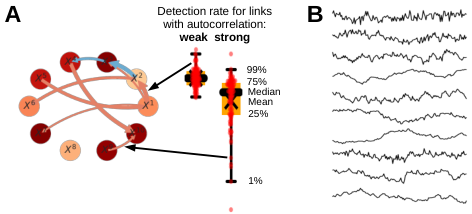
Here we model four of the major challenges of time series from complex systems such as the Earth: High-dimensionality, time lagged causal dependencies, autocorrelation, and potentially strong nonlinearity. Fig. 4A gives an example model for variables and Fig. 4B shows a time series realization illustrating some strongly autocorrelated variables. We create a number of models with different random network topologies of time series variables with each network having linear or nonlinear causal dependencies (except for the bivariate case with ). From each of these models, we generate time series datasets (each of length ) to assess true and false positive rates of individual causal links in a model with the different causal methods. As illustrated in Fig. 4A the boxplots in the following figures show the distribution of these individual link false and true positive rates across the large variety of random networks, for each network size differentiated between weakly and strongly autocorrelated pairs of variables in the left and right boxplot, respectively (defined by the average autocorrelation of both variables being smaller or larger than ). The full model setup is detailed in Supplementary Sect. S4, Tab. S3 lists the experimental setups, and Tab. S4 gives details on the compared methods.
Experiments with linear relationships
In Fig. 4C we first investigate the performance of linear causal discovery methods on numerical experiments with linear causal links. The setup has a sample length of observations and all cross-links have the same coupling coefficient and, hence, the same causal effect strength. Next to correlation (Corr) and FullCI (here implemented with an efficient vector-autoregressive model estimator), we compare PCMCI with the original PC algorithm as a standalone method and Lasso regression as the most widely used representative of regularized high-dimensional regression techniques that can be used for causal variable selection. Table S4 gives an overview over the compared methods, implementation details for alternative methods are given in Supplementary Sect. S1.2. The maximum time lag is for all methods.
Correlation is obviously inadequate for causal discovery with very high false positive rates (first column in Fig. 4C). But even detection rates for true links vary widely with some links with under 20% true positives, despite the equal coefficients for all causal links. This counterintuitive result is further investigated in Fig. 6. In contrast, all causal methods control false positives well around or below the chosen 5% significance level with Lasso and the PC algorithm overcontrolling at lower than expected rates. An exception here are some highly autocorrelated links which are not correctly controlled with the PC algorithm (whiskers extending to 25% false positives in Fig. 4C) since it does not appropriately deal with the time series case.
While FullCI has a detection power of around 80% for , this rate drops to 40% for and FullCI cannot be applied anymore for larger when the dimensionality is larger than the sample size (). But also for some links between strongly autocorrelated variables have a detection rate of just 60%. Lasso has higher detection power than FullCI on average and the PC algorithm interestingly displays not much difference in detection power between and , but the rates are lower than for Lasso on average, and higher autocorrelation also here has a detrimental effect.
PCMCI robustly shows high detection power even for network sizes with dimensions exceeding the sample size and displays almost the same power for links with the same causal effect, regardless of whether autocorrelations are weak or strong, up to . The second last column in Fig. 4C depicts the detection rates for the condition-selection step PC1: Until still more than 80% of the true parents are detected (black line). As mentioned, PC1 is tuned to high power and for more than 80% of the selected conditions are false positives (red line), but still the number of conditions is only a small fraction (grey line) of the conditions used for FullCI.
Runtime depends on implementation details, but all methods are in the same order of magnitude except for FullCI. Theoretically, in the worst case PCMCI scales polynomially with and . Our numerical experiments show that for smaller networks, PCMCI is faster than Lasso. Most of the time of PCMCI is spent on the condition-selection step, mainly because of the hyperparameter optimization of via AIC. Fixing is much faster and still gives good results (Figs. S3,S4), but may not always control false positives. The runtime of the standalone PC algorithm strongly depends on the number of conditioning sets tested. In theory all combinations of conditioning sets are tested which makes PC extremely slow and leads to a highly varying runtime, but here we limited the number of combinations (see Supplementary Sect. S1.2).
Summarizing, our key result here is that PCMCI has high power even for network sizes with dimensions, given by , exceeding the sample size. Average power levels (marked by ‘x’ in Fig. 4C) are higher than FullCI and PC for all considered network sizes. PCMCI has similar average power levels compared to Lasso, but an important difference is the worst-case performance: Even for small networks (), a significant part of the links is constantly overlooked with Lasso, while for PCMCI 99% of the links have a detection power greater than 70%.
Experiments with nonlinear relationships
Figure 5 displays results for nonlinear models where we differentiate between linear and two types of nonlinear links (upper three rows). In essence, here we find that PCMCI’s ability to avoid high-dimensionality is even more crucial not only for detection power, but also to control false positives correctly.
In Fig. 5A, FullCI, PC, and PCMCI are all implemented with the GPDC conditional independence test and dCor denotes the distance correlation as the nonlinear analog to correlation (see Tab. S2). Distance correlation alone detects nonlinear links, but does not account for indirect or common driver effects leading to high false positives, especially for strong autocorrelation. FullCI here works well only up to , but cannot control false positives anymore for since the GPDC test does not work well in high dimensions. PC overcontrols false positives again (except for strong autocorrelation) and has the lowest power levels among all methods. PCMCI has the highest power levels which only slightly decrease for larger networks. Here we find that for nonlinear links weakly and strongly autocorrelated links also have different power levels, unlike for linear links (further discussed in Supplementary Sect. S3). False positives are mostly controlled correctly, but there is a slight inflation of false positives for larger networks, again because even with condition-selection the dimensionality increases for larger networks and GPDC does not work well in high-dimensions. For GPDC, runtime for PC and PCMCI is larger than for FullCI.
Figure 5B depicts results for the fully non-parametric implementation with CMI. Then FullCI has the slowest runtime and almost no power, especially for nonlinear links, while PCMCI controls false positives correctly and has a higher power than PC except for some types of nonlinear links.
Causal strength experiments
Finally, in Fig. 6 we more systematically investigate the close relationship between detection power and causal effect size illustrated in the climate example. In particular, we show that PCMCI has higher effect size than FullCI and often even higher effect size than correlation and, thus, more power.
Different from the model setup before, we now fix a network size of time series variables and vary the link coefficients (-axis in Fig. 6). The (standardized) causal effect is (black line). The bottom row of Fig. 6 depicts the distribution of effect sizes, that is, correlation, FullCI partial correlation, and MCI partial correlation across the different links for various random network topologies. Correlation values for links with the same causal effect span the whole range from zero to high correlation values indicating that correlation is rather unrelated to causal effect strength. Some correlation values are much smaller and even tend to zero which provides evidence for the observation that the detection power of correlation (or the other unconditional measures dCor and MI) can, counter-intuitively, even be lower than that of FullCI or PCMCI. The distribution of FullCI values is much narrower, but tends to be smaller than causal strength. In Supplementary Sect. S3 we provide proofs that MCI is larger than FullCI and that MCI is an estimator of causal strength as confirmed by our numerical experiments. In sum, larger effect size and lower dimensionality lead to more detection power of PCMCI compared to FullCI.
Further experiments
In the Supplementary Material we investigate some further methodological variants and show that our results are robust also for larger sample sizes (Supplementary Figs. S3,S4,S8,S10,S12), higher network coupling densities (Figs. S5,S6), and observational noise (Fig. S13). All methods display a similar sensitivity to observational noise with levels up to 25% of the dynamical noise standard deviation having only minor effects. For levels of the same order as the dynamical noise we observe a stronger degradation with also the false positives not being correctly controlled anymore since common drivers are essentially not well detected anymore. See ref. [37] for a discussion on observational noise.
Discussion and conclusion
Causal discovery on large-scale time series datasets is plagued by a dilemma: Including more variables makes an analysis more credible regarding a causal interpretation, but if the added variables are irrelevant, that is, not explanatory for the observed relationships, they not only increase dimensionality but may also lead to smaller effect sizes. Both of these factors lead to lower power and increase the risk that important true causal links are overlooked. Furthermore, some nonlinear tests do not even control false positives anymore in high dimensions.
Our method circumvents this problem by a condition-selection step to remove irrelevant variables and a conditional independence test designed for highly interdependent time series. The former improves power levels for large-scale causal discovery analyses, while the latter also yields more power than classical techniques in analyses involving only few variables implying an improved ‘causal signal-to-noise ratio’. At the same time the MCI test demonstrates correctly controlled false positive rates even for highly autocorrelated time series data. Furthermore, MCI can be interpreted as a measure of causal strength, allowing to rank causal links in exploratory studies on large datasets with many time series in a meaningful way. Such rankings can help to identify the strongest inferred causal links, which may be of main interest in some domain contexts.
PCMCI allows accommodating a large variety of conditional independence tests adapted to different types of data (see Sect. S2), for example, discrete or continuous time series. Networks can also be reconstructed with multivariate variables as nodes in the graph. This flexibility can help to represent causal associations on different aggregation levels and opens up a way to study causal networks on multiple interdependent layers[38].
Our method focuses on time-lagged dependencies, where there is no ambiguity in terms of cause-effect directionality. Recently, a growing body of literature addresses the inference of causality without relying on time-lags [39, 40] which could help to determine causal directionality for contemporaneous links.
For a causal interpretation, our approach rests on the standard assumptions [18] of Causal Sufficiency, implying that all common drivers are observed, and the Causal Markov Condition, stating that once we know the direct causes of a variable, all other variables in the past become irrelevant for prediction, among other, more technical, assumptions. See ref. [37] for an overview over causal discovery in time series. Causal Sufficiency implies that the term ‘causal’, as we use it here, has to be understood relative to the set of included variables. Non-included variables can still be the cause of a link in a non-experimental analysis. But the causal links inferred from the available observational data can then yield new hypotheses to be rejected or confirmed by further data analyses involving more variables (as illustrated in our climate example) or model simulations. On the other hand, the finding of non-causality, that is, the absence of a causal link, relies on weaker assumptions[37]. Given that the observed data faithfully represents the underlying process and that potential nonlinearities are powerfully enough captured by the dependence measure, the absence of evidence for a statistical relationship makes it unlikely that a linking physical mechanism in fact exists. Such findings of non-causality are, therefore, more robust.
Growing data availability promises an unprecedented opportunity for novel insights through causal discovery across all disciplines of science. But current causality methods have been mostly limited to bivariate analyses that make a causal interpretation less credible. Our novel method enables multivariate causal analyses opening up new possibilities to more credibly reconstruct causal networks.
Materials and Methods
The main text describes the novel method introduced, some further material can be found in the Supplement. Software to reproduce the examples and numerical experiment results is available online under
https://github.com/jakobrunge/tigramite
including a comprehensive documentation of the method.
References
- [1] IPCC, Climate Change 2013: The Physical Science Basis. Contribution of Working Group I to the Fifth Assessment Report of the Intergovernmental Panel on Climate Change (Cambridge University Press, Cambridge, 2013).
- [2] D. Baldocchi, ’Breathing’ of the terrestrial biosphere: lessons learned from a global network of carbon dioxide flux measurement systems. Aust. J. Bot. 56, 1 (2008).
- [3] T. J. Mosedale, D. B. Stephenson, M. Collins, T. C. Mills, Granger causality of coupled climate processes: Ocean feedback on the North Atlantic Oscillation. J. Clim. 19, 1182–1194 (2006).
- [4] A. Attanasio, A. Pasini, U. Triacca, A contribution to attribution of recent global warming by out-of-sample Granger causality analysis. Atmos. Sci. Lett. 13, 67–72 (2012).
- [5] C. Papagiannopoulou, et al., A non-linear Granger-causality framework to investigate climate-vegetation dynamics. Geosci. Model Dev. 10, 1945–1960 (2017).
- [6] M. C. McGraw, E. A. Barnes, Memory matters: A case for Granger causality in climate variability studies. J. Clim. in press, JCLI–D–17–0334.1 (2018).
- [7] E. Bullmore, O. Sporns, Complex brain networks: graph theoretical analysis of structural and functional systems. Nat. Rev. Neurosci. 10, 186–98 (2009).
- [8] A. K. Seth, A. B. Barrett, L. Barnett, Granger Causality Analysis in Neuroscience and Neuroimaging. J. Neurosci. 35, 3293–3297 (2015).
- [9] C. W. J. Granger, Investigating causal relations by econometric models and cross-spectral methods. Econometrica 37, 424–438 (1969).
- [10] L. Barnett, A. K. Seth, Granger causality for state space models. Phys. Rev. E 91, 040101 (2015).
- [11] R. Tibshirani, Regression shrinkage and selection via the lasso. J R Stat Soc Ser. B Stat Methodol 58, 267–288 (1996).
- [12] H. Zou, The Adaptive Lasso and Its Oracle Properties. J. Am. Stat. Assoc. 101, 1418–1429 (2006).
- [13] I. Ebert-Uphoff, Y. Deng, Causal discovery for climate research using graphical models. J. Clim. 25, 5648–5665 (2012).
- [14] J. Runge, V. Petoukhov, J. Kurths, Quantifying the Strength and Delay of Climatic Interactions: The Ambiguities of Cross Correlation and a Novel Measure Based on Graphical Models. J. Clim. 27, 720–739 (2014).
- [15] M. Kretschmer, D. Coumou, J. F. Donges, J. Runge, Using causal effect networks to analyze different arctic drivers of midlatitude winter circulation. J. Clim. 29, 4069–4081 (2016).
- [16] P. Spirtes, C. Glymour, An Algorithm for Fast Recovery of Sparse Causal Graphs. Soc. Sci. Comput. Rev. 9, 62–72 (1991).
- [17] J. Pearl, Causality: Models, Reasoning, and Inference (Cambridge University Press, Cambridge, 2000).
- [18] P. Spirtes, C. Glymour, R. Scheines, Causation, Prediction, and Search (The MIT Press, Boston, 2000).
- [19] F. Bach, Consistency of the group Lasso and multiple kernel learning. J. Mach. Learn. Res. 9, 1179–1224 (2008).
- [20] R. Lockhart, J. Taylor, R. Tibshirani, R. Tibshirani, A significance test for the lasso. Ann. Stat. 42, 413–468 (2014).
- [21] J. Taylor, R. J. Tibshirani, Statistical learning and selective inference. Proc. Natl. Acad. Sci. 112, 7629–34 (2015).
- [22] N. A. Rayner, et al., Global analyses of sea surface temperature, sea ice, and night marine air temperature since the late nineteenth century. J. Geophys. Res. 108, 4407 (2003).
- [23] P. J. Nowack, P. Braesicke, N. Luke Abraham, J. A. Pyle, On the role of ozone feedback in the ENSO amplitude response under global warming. Geophys. Res. Lett. 44, 3858–3866 (2017).
- [24] C. F. Ropelewski, M. S. Halpert, North American Precipitation and Temperature Patterns Associated with the El Niño/Southern Oscillation (ENSO). Mon. Weather Rev. 114, 2352–2362 (1986).
- [25] A. Shabbar, M. Khandekar, The impact of el Nino-Southern oscillation on the temperature field over Canada: Research note. Atmos. - Ocean 34, 401–416 (1996).
- [26] M. Eichler, Graphical modelling of multivariate time series. Probab. Theory Relat. Fields 153, 233–268 (2012).
- [27] J. Runge, J. Heitzig, V. Petoukhov, J. Kurths, Escaping the Curse of Dimensionality in Estimating Multivariate Transfer Entropy. Phys. Rev. Lett. 108, 258701 (2012).
- [28] C. F. Aliferis, A. Statnikov, I. Tsamardinos, S. Mani, X. Koutsoukos, Local Causal and Markov Blanket Induction for Causal Discovery and Feature Selection for Classification Part I: Algorithms and Empirical Evaluation Ioannis Tsamardinos. J. Mach. Learn. Res. 11, 171–234 (2010).
- [29] C. Rasmussen, C. Williams, Gaussian processes for machine learning (MIT Press, Cambridge, MA, USA, 2006).
- [30] G. J. Székely, M. L. Rizzo, N. K. Bakirov, Measuring and testing dependence by correlation of distances. Ann. Stat. 35, 2769–2794 (2007).
- [31] J. Runge, Proc. 21st Int. Conf. Artif. Intell. Stat. (2018).
- [32] J. M. Robins, R. Scheines, P. Spirtes, L. Wasserman, Uniform consistency in causal inference. Biometrika 90, 491–515 (2003).
- [33] M. Kalisch, Estimating high-dimensional directed acyclic graphs with the PC-algorithm. J. Mach. Learn. Res. 8, 613–636 (2007).
- [34] B. Pompe, J. Runge, Momentary information transfer as a coupling measure of time series. Phys. Rev. E 83, 1–12 (2011).
- [35] J. Runge, Quantifying information transfer and mediation along causal pathways in complex systems. Phys. Rev. E 92, 062829 (2015).
- [36] J. Runge, Causal network reconstruction from time series: From theoretical assumptions to practical estimation. Chaos in press (2018).
- [37] S. Boccaletti, et al., The structure and dynamics of multilayer networks. Phys. Rep. 544, 1–122 (2014).
- [38] P. Spirtes, K. Zhang, Causal discovery and inference: concepts and recent methodological advances. Appl. Informatics 3, 3 (2016).
- [39] J. Peters, D. Janzing, B. Schölkopf, Elements of causal inference: foundations and learning algorithms, no. December (MIT Press, Cambridge, Massachusetts, 2017).
- [40] P. D. Jones, et al., Hemispheric and large-scale land-surface air temperature variations: An extensive revision and an update to 2010. J. Geophys. Res. Atmos. 117 (2012).
Acknowledgments
We thank G. Balasis, D. Coumou, J. Donges, F. Fröhlich, J. Haigh, J. Heitzig, J. Kurths, M. Mengel, M. Reichstein, C.-F. Schleussner, E. van Sebille, K. Zhang, and J. Zscheischler for helpful discussions and comments. The authors thank C. Linstead for help with high-performance computing.
Funding
J.R. received funding from a postdoctoral award by the James S. McDonnell Foundation. The work was supported by the European Regional Development Fund (ERDF), the German Federal Ministry of Education and Research and the Land Brandenburg for supporting this project by providing resources on the high-performance computer system at the Potsdam Institute for Climate Impact Research. We declare no conflicts of interest.
Author contributions
J.R. designed the method, analyzed the data, and prepared the manuscript. D.S. contributed to mathematical formulation, M.K. contributed to the climate analysis. All authors discussed the results and contributed to editing the manuscript.
Supplementary Materials
Further material that can be found in the Supplement.
Supplementary Material: Detecting causal associations in large nonlinear time series datasets
Jakob Runge, Peer Nowack, Marlene Kretschmer, Seth Flaxman, and Dino Sejdinovic
S1 Causal discovery
In this section we describe the proposed causal discovery method PCMCI as well as alternative techniques in more detail.
S1.1 Causal discovery method (PCMCI)
In our framework, the dependency structure of a set of time series variables is represented in a graphical model [41]. While the process graph depicted in Fig. 1B is easier to visualize, it does not fully represent the spatio-temporal dependency structure underlying complex dynamical systems which is more comprehensively grasped in a time series graph [27] as shown in Fig. 3. If, for example, graphical models are estimated without taking into account lagged variables, associations can easily be confounded by the influence of common drivers at past times.
Definition 1 (Definition of time series graph).
Let be a multivariate discrete-time stochastic process and the associated time series graph. The set of nodes in that graph consists of the set of components at each time . The edges of the graph are defined as follows: Variables and are connected by a lag-specific directed link “” in pointing forward in time if and only if and
| (S1) |
where ‘’ denotes the absence of a conditional independence and the past of the multivariate process excluding .
That is, the graph is actually infinite, but in practice estimated up to some maximum time lag . Throughout this work we assume stationarity, the links are repeated for every if a link exists at time . The parents of a node are defined as
| (S2) |
In summary, the parents for all variables define the graph . Contemporaneous dependencies for can be defined in different ways [36]. Here they are left undirected, but other techniques [40, 39] could be applied to determine causal directionality for contemporaneous links.
Our causal discovery technique to estimate the time series graph is based on a two-step procedure:
- 1.
Condition-selection: Obtain an estimate of (a superset of) the parents for all variables with Algorithm S1.
- 2.
Use these parents as conditions in the MCI causal discovery Algorithm S2, which tests all variable pairs with and time-delay and establishes a link, that is, , if and only if
(S3) where denotes the strongest parents according to the sorting in Algorithm S1. This parameter is just an optional choice. One can also restrict the maximum number of parents used for , but here we impose no restrictions. For one can also consider undirected contemporaneous links [36].
Both the conditional independence tests in the condition-selection step and the MCI test can be implemented with different test statistics as detailed in Sect. S2 and Tab. S2.
Algorithm S1 in the first step is a variant of the skeleton-discovery part of the PC algorithm [16] in its more robust modification called PC-stable [42] and adapted to time series. The algorithm then is as follows: For every variable the algorithm starts by initializing the preliminary parents . Then we start with and iteratively remove a variable from if the null hypothesis
| (S4) |
is accepted at a significance threshold , where are different combinations of subsets of with cardinality up to a maximum number of combinations . In the first step (), is empty and we, thus, test unconditional dependencies. In each next step, the cardinality is increased and Eq. S4 is tested again for different combinations of . The algorithm converges for a link once and the null hypothesis is rejected (if the null hypothesis is accepted, the link is removed). Our fast variant PC1 is obtained by restricting the maximum number of combinations per iteration to . Further, we sort after every iteration according to the test statistic value (ParCorr, GPDC or CMI) and pick in lexicographic order, that is, for , only the conditions with highest association. Other causal variable-selection algorithms employ similar heuristics [30, 43, 44]. The MCI step is inspired by the information-theoretic measure momentary information transfer introduced in [35, 45].
| Parameter | Description | Recommended values |
| Significance threshold in pre-selection Algorithm S1 | ParCorr: by AIC GPDC, CMI: | |
| Max. number of parents of in Algorithm S2 | unrestricted (but can be as low as 1, see discussion) | |
| Max. time delay in Algorithms S1,S2 | last lag with significant unconditional association |
As listed in Tab. S1, the free parameters of this method (in addition to free parameters of the conditional independence test statistic) are the maximum time delay , the significance threshold , and the maximum number of conditions of the driver variable in Algorithm S2. We abbreviate different parameter choices by PC+MCI, if not clear from the context. In Fig. S7 we show the overall performance of PCMCI for different choices of . In the present implementation we do not take into account the reduced degrees of freedom in the MCI test due to the condition-selection step. We have not found any sign of inflated false positives in our numerical experiments. However, in order to ensure a more conservative false positive control, one could split the dataset and conduct the condition-selection on a separate part of the dataset than that used for the MCI tests. This would, however, clearly lead to a decrease in power and carry the problem of choosing the split in time series.
Choice of
The maximum time delay depends on the application and should be chosen according to the maximum physical time lag expected in the complex system. In practice we recommend a rather large choice that includes peaks in the lagged cross-correlation function (or a more general measure corresponding to the chosen independence test), because a too large choice of merely leads to longer runtimes of PCMCI, but not to an increased estimation dimension as for FullCI.
Choice of
should not be seen as a significance test level in PC1 since the iterative hypothesis tests do not allow for a precise assessment of uncertainties. here rather takes the role of a regularization parameter as in model-selection techniques. The conditioning sets estimated with PC1 should include the true parents and at the same time be small in cardinality to reduce the estimation dimension of the MCI test and improve its power. But the first demand is typically more important. In Fig. S7 we investigate the performance of PCMCI implemented with ParCorr, GPDC, and CMI for different . Too small values of result in many true links not being included in the condition set for the MCI tests and, hence, increase false positives. Too high levels of lead to high dimensionality of the condition set which reduces detection power and increases the runtime. Note that for a threshold in Algorithm S1, no parents are removed and all variables would be selected as conditions. Then the MCI test becomes a FullCI test. As in any variable-selection method [30, 43], can be optimized using cross-validation or based on scores such as BIC or AIC. For all ParCorr experiments (except for the ones labeled with PC+MCI), we optimized with AIC as a selection criterion. More precisely, for each we ran PC1 separately for each yielding different conditioning sets . Then we fit a linear model for each
| (S5) |
yielding the residual sum of squares (RSS) and select according to Akaike’s Information criterion modulo constants
| (S6) |
where is the sample size (typically the time series length minus a cutoff due to ) and denotes cardinality. For GPDC one can similarly select based on the log marginal likelihood of the fitted Gaussian process, while for CMI one can use cross-validation based on nearest-neighbor predictions for different . But since GPDC and CMI are already quite computationally demanding, we picked in all experiments based on our findings in Fig. S7. In the lower panels of Figs. S3,S4,S5,S6 we analyzed also for ParCorr for all numerical experiments and found that this option also gave good results for sparse networks and runs even faster than Lasso. For very dense networks, we, however, found inflated false positives. Unfortunately, we have no finite sample consistency results for choosing .
Choice of
While the parents are sufficient to assess conditional independence, the additional conditions are used to account for autocorrelation and make the MCI test statistic a measure of causal strength as analyzed in Sect. S3. To limit high dimensionality, one can strongly restrict the number of conditions with the free parameter . To avoid having another free parameter, we kept unrestricted in most experiments, but in our tests we found that a small value or already suffices to reduce inflated false positives due to strong autocorrelation and estimate causal strength, resulting in a confined scaling of power with link strength. The reason is that typically the largest driver will be the autodependency and conditioning out its influence already diminishes the effect of strong autocorrelations.
In the lower panels of Figs. S3,S4,S5,S6 we found that PCMCI with is slightly faster and yields more power. It also leads to a smaller power difference between weakly and strongly autocorrelated links than with MCIall. In theory, a too small does not guarantee a well-calibrated test (see Sect. S3.3), but in practice it seems like a sensible tradeoff.
False discovery rate control
PCMCI can also be combined with false discovery rate controls, e.g., using the Hochberg-Benjamini approach [46]. This approach controls the expected number of false discoveries by adjusting the -values resulting from the MCI step for the whole time series graph. More precisely, we obtain the -values as
| (S7) |
where is the original p-value, is the rank of the original p-value when p-values are sorted in ascending order, and is the number of computed p-values in total, that is, to adjust only directed links for and correspondingly if also contemporaneous links for are taken into account. The false discovery approach controls the expected proportion of discoveries (rejected null hypotheses) that were false. In our numerical experiments we did not control the false discovery rate since we are interested in the individual link performances.
S1.2 Alternative methods
Here we define alternative causal and non-causal methods, Tab. S4 gives an overview over the methods compared in the numerical experiments.
S1.2.1 FullCI
The most straightforward way to test the existence of causal links as defined in Def. (1) is to directly test
| (S8) |
where denotes the multivariate process and its past. In practice, the past is truncated at a maximum time lag . This test can be implemented with any of the conditional independence tests defined in Sect. S2
In its original formulation, Granger causality between time series variables and is based on fitting a linear or nonlinear model including possible confounders to and a causal link is assessed by quantifying whether the inclusion of the past of variable in the model significantly reduces the prediction error about [9]. Our formulation can be interpreted as a general, lag-specific version. For linear models we implement FullCI by fitting a vector-autoregressive (VAR) model using the statsmodels package which also allows to obtain the corresponding p-values.
S1.2.2 Lasso
In the linear case, FullCI can be phrased as testing for nonzero coefficients in a VAR model. If implemented using standard ordinary least-square regression, the problem becomes ill-defined if the number of coefficients exceeds the number of samples. One way to address this problem are regularized high-dimensional regression techniques. In particular, Lasso[11] is a common regression method that can also be used for variable selection. Lasso regression is known to be inconsistent in some scenarios which is overcome by the adaptive Lasso[12] which yields a consistent estimator by utilizing an adaptively weighted penalty. Here we implemented an adaptive Lasso that consists of computing several Lasso regressions with iterative feature reweighting, see Algorithm S3. After several iterations the active set of variables is determined as the non-zero coefficients. Then all zero-coefficients are assigned a p-value of one, while the p-values for the active set of variables is determined by an OLS regression including only the active variables. To select the optimal regularization parameter we used a time-series based cross-validation scheme. Some tests based on AIC-selected hyperparameters did not yield good results.
S1.2.3 PC algorithm
The original PC algorithm was formulated for general random variables without assuming a time order. It consists of several phases where first, in the skeleton-discovery phase, an undirected graphical model [41] is estimated whose links are then oriented using a set of rules [16, 18]. We implement the skeleton-discovery phase of the PC algorithm as given in Algorithm S1, but in contrast to our fast variant, the original version does not restrict the number of condition combinations to test. Here we use a large choice of . In contrast to FullCI or PCMCI, it is not straightforward to assess the confidence of causal links with the PC algorithm because links are iteratively removed. Here we use a -value assessment for causal links according to ref. [47],
| (S9) |
that is, the maximum of all -values from the conditional independence tests for different condition sets in Eq. S4 defines the aggregated -value of a causal link. This causal discovery method we term PC in the numerical experiments. We found that the -values tend to be over-conservative for the most part with outliers for strong autocorrelations. FPR levels cannot be reliably controlled just below a desired threshold.
S1.2.4 PCMCI variants
In the MCI step of the PCMCI method, one can also test
| (S10) |
for all links, that is, the MCI test without the condition on the parents , or, equivalently, , denoted PC1+MCI0. Note that for this is the test in the last step of the PC algorithm, but here also links that were removed in Algorithm S1 are tested again. In our numerical experiments (Figs. S3,S4,S5,S6) we found that PC1+MCI0 has inflated false positives.
We also test a variant, called PC1+MCI0pw, where all time series are pre-whitenend prior to running PC1+MCI0, that is, we preprocessed all time series by estimating the univariate lag-1 autocorrelation coefficients and regressing out the AR(1) autocorrelation part of the signals:
| (S11) |
Then the PCMCI test is applied to these residuals . Our numerical results in Figs. S3,S4,S5,S6 show that this approach also fails to control false positives.
For conditional mutual information as a test statistic, MCI0 was called information transfer to Y (ITY) in ref. [45]. For a link , it quantifies the unique information in entering a process without excluding the information in the past of . ITY and the information-theoretic version of MCI called momentary information transfer (MIT) are part of a whole suite of measures to quantify causal information flow in complex systems [36]. Another measure called ITX quantifies the unique information emanating from a process as an information-theoretic analog to Sims causality, and several other measures quantify mediation on information pathways as discussed in ref. [36].
S1.2.5 BivCI
In the numerical experiments, we also evaluate a bivariate conditional independence test (BivCI),
| (S12) |
where denotes the past of . This corresponds to a pairwise lag-specific version of Granger causality or Transfer Entropy[48]. Thus, this test removes autocorrelation to some extent, but does not exclude common drivers or indirect dependencies. Also autodependencies induced by common drivers are not removed. As analyzed in Figs. S3,S4,S5,S6 BivCI reduces autocorrelation effects to some extent, but false positives are not correctly controlled, as expected.
S1.2.6 Unconditional pairwise measures
We also investigate the unconditional pairwise measures . In the ParCorr implementation this is simply the Pearson correlation coefficient (Corr), in the GPDC implementation the distance correlation (dCor), and for CMI the mutual information (MI).
S2 Conditional independence tests
Similarly to the PC algorithm, the PCMCI framework (Algorithm S1 and S2) that we propose can be used in conjunction with any conditional independence test – these will typically be based on estimating different dependence measures with associated test statistics. Here we implement three tests: partial correlation (ParCorr), a nonlinear two-step conditional independence test we term GPDC, and a fully non-parametric test based on conditional mutual information[29]. Table S2 gives an overview over the tests.
S2.1 ParCorr
Partial correlation for testing here is estimated (Tab. S2) in a two-stage procedure with a multivariate regression of and on followed by a correlation test on the residuals. Its advantages are fast computation and that the distribution under the null hypothesis of conditional independence is known analytically, but it is applicable only to the multivariate Gaussian case which can only capture linear dependencies.
S2.2 GPDC
GPDC also belongs to the class of residual-based conditional independence tests. Instead of a linear regression, here the first step is a Gaussian process (GP) regression [31] and the second step a test for the (unconditional) independence of the uniformized residuals with the distance correlation coefficient [32]. GP regression is a widely used Bayesian nonparametric regression approach. Distance correlation[32] is a measure of dependence between two random variables and is zero if and only if the variables are independent. Thus, distance correlation measures both linear and nonlinear association. See Tab. S2 for details. Note that the underlying assumption of GPDC is that of an additive functional dependency, see ref. [49] for a more general, but still residual-based, test.
The estimator for distance correlation is defined as
| (S13) |
where the distance covariance and variance are computed by
| (S14) |
where are the doubly-centered distance matrices of and (see ref. [32]), respectively, and is the sample size (in the present context the length of the time series minus cutoffs due to ). Distance correlation is implemented in Tigramite based on the code in the original dcov.test function in the energy package for the R-language. The prior transformation of and to uniform marginals allows to pre-compute the distribution for each sample size (implemented in Tigramite) and critical values under the independence null hypothesis – thereby avoiding computationally expensive permutation tests for each test of . Note that since we are not aware of a way to account for the GP-step in assessing the degrees of freedom for the subsequent distance correlation, we simply used the sample size which did not seem to inflate false positives in our experiments.
Figure 3D illustrates a quadratic relationship and for where can be identified with GPDC, but not with ParCorr.
S2.3 CMI
ParCorr and GPDC, like any two-step procedure for conditional independence testing, which includes a regression followed by an unconditional test on the regression residuals, has an underlying assumption of additive noise and a functional dependence on the conditioning variables. In the presence of dependencies which cannot be represented even in a nonlinear functional form, regression will not be able to remove these dependencies on the conditioning variables. Figure 3D for CMI illustrates a multiplicative case with and for where both ParCorr and GPDC fail to establish . Then the two-step procedure should be replaced with fully non-parametric techniques to measuring and testing conditional dependence.
Here a fully non-parametric test[29] for continuous data based on conditional mutual information combined with a local permutation scheme is implemented. The conditional mutual information (CMI) is zero if and only if . From the nearest-neighbor entropy estimator by Kozachenko et al.[50], Kraskov et al.[51] developed an estimator for mutual information that was generalized to CMI[52, 53]:
| (S15) |
with the Digamma function as the logarithmic derivative of the Gamma function and sample length . The only free parameter is the number of nearest neighbors in the joint space of which defines the local length scale (in maximum norm) around each sample point . Then , and are computed by counting the number of points with distance strictly smaller than (including the reference point ) in the subspace to get , in the subspace to get , and in the subspace to get . The decisive advantage of this estimator compared to fixed global bandwidth approaches is its local data-adaptiveness (Fig. 3D): The hypercubes around each sample point are smaller where more samples are available. As opposed to GP regression, this feature allows to detect also highly non-smooth dependencies. Unfortunately, few theoretical results are available for the complex mutual information estimator. While the Kozachenko-Leonenko estimator is asymptotically unbiased and consistent [50, 54], the variance and finite sample convergence rates are unknown. Hence, the null distribution in the CMI test relies on a local permutation test that is also based on nearest neighbors and data-adaptive. Here we set , and the nearest neighbors in the local permutation scheme, , as well as as the number of surrogates for the null distribution. These choices are based on the findings in ref. [29]. CMI is implemented in Tigramite. Alternative conditional independence tests are, e.g., kernel conditional independence tests [55, 56, 57]. PCMCI-CMI can be considered a doubly adaptive causal discovery method: PCMCI adapts the condition-selection locally to the causal network and CMI adapts the conditional independence estimation locally to the sample density.
S2.4 Discrete data
The previous tests were developed for continuously-valued data. For discrete data, the software package Tigramite implements a CMI test based on discrete entropy estimation, called CMIsymb. This test directly estimates CMI based on
| (S16) |
where the discrete densities are estimated from symbol frequencies. For this test no analytical results for the null distribution are available and a permutation test is recommended.
S2.5 Multivariate extensions
We note that we focus on the case of univariate time series and as is typical in causal discovery applications (while the conditioning variable can and mostly will be multivariate). However, our method can be readily extended to multivariate time series and , as well as those taking values in structured or non-Euclidean domains for suitable conditional independence tests. CMI, for example, readily extends to multivariate and . Also a two-step procedure involving vector-valued regression and kernel conditional independence tests [55, 56, 58] can be used. In complex dynamical systems, multivariate variables can, for example, result from delay-embeddings to better unfold the dynamics of nonlinear systems [59]. Or, one can create multivariate variables from aggregating time series of multiple subprocesses to represent a dynamical process on a higher layer [60]. Causal networks reconstructed on such different layers then lend themselves to analysis with measures from the growing field of multilayer networks [38].
S3 Properties of PCMCI
In this section, we provide more formal definitions and proofs for the properties of PCMCI stated in the main article.
S3.1 Computational complexity
PCMCI has polynomial worst case complexity in the number of variables and . The computational complexity of the first step of PCMCI (Algorithm S1) strongly depends on the network structure and the parameter . The sparser the causal dependencies, the faster the convergence. In the worst case where the network is completely connected (which is rather pathological), the computational complexity of the PC1 condition-selection step for variables amounts to
| (S17) |
conditional independence tests with iteratively increasing cardinality. The MCI step (Algorithm S2) further involves tests (for ) of a maximal dimensionality of . Hence the worst case total computational complexity in the number of variables is polynomial and given by if -optimization is not taken into account. The computational time will then depend on how the conditional independence test scales with this dimensionality and the time series length . In the numerical experiments, we analyze runtimes of the different techniques for different network sizes and time series lengths .
In Tigramite we implement a recycle_residuals-option that can be used for ParCorr and GPDC to save already computed residuals in memory to be reused in later tests of PC1 or MCI.
S3.2 Consistency
We here give a proof of the consistency of PCMCI for the population version of PCMCI, that is, PCMCI estimates the true graph in the limit of infinite sample size where there are no errors in the conditional independence tests. The proof relies on the three standard assumptions in causal discovery[18]: (1) Causal Sufficiency implying that there exist no other unobserved variables that directly or indirectly influence any other pair of our set of observed variables, (2) the Causal Markov Condition implying that is independent of given its parents , and (3) Faithfulness which guarantees that the graph entails all conditional independence relations that are implied by the Markov condition. Faithfulness implies that if two variables are independent conditionally on a set , then they are also separated by in the graph. See ref. [36] for definitions of separation in time series graphs. As part of the Causal Markov Condition in the time series graph context, we also assume no-contemporaneous causal effects which excludes causal effects at . Only then the lagged parents are sufficient for the Causal Markov condition. Last, we also assume stationarity here for all the time series considered so that dependencies (or lack of them) remain unchanged across time. With these assumptions we can prove the consistency of PCMCI.
Theorem 1.
(Consistency) Let be a stochastic process with true time series graph as defined in Def. 1 and let be the estimated graph with PCMCI (Algorithms S1,S2) implemented with a consistent conditional independence test. Assuming Causal Sufficiency, Faithfulness and the Causal Markov Condition we have that
| (S18) |
To prove consistency, we need the following two lemmas.
Lemma 1.
Let denote the estimated condition set of Algorithm S1 for and let denote the true parents. Assuming Faithfulness and Causal Sufficiency with a consistent conditional independence test in the limit of infinite sample size we have that
| (S19) |
that is, the estimated parents are a superset of the true parents.
Proof.
Suppose . Causal Sufficiency implies that was observed and independence can be tested. For (default parameter value in PC1) and with a consistent conditional independence test in the limit of infinite sample size PC1 removes from if and only if in the last step of PC1. Now Faithfulness implies that then and hence . ∎
Lemma 1 holds assuming only Causal Sufficiency and Faithfulness. If we additionally assume the Causal Markov Condition, PC1 estimates exactly the true parents.
Lemma 2.
Let denote the estimated condition set of Algorithm S1 for . Assuming Faithfulness, the Causal Markov Condition and Causal Sufficiency in the limit of infinite sample size we have that
| (S20) |
that is, the estimated parents are the true parents.
Proof.
From Lemma 1 we know that is a superset of , so we only need to check whether all parents in are also in . Assume the contrary that , but . The contraposition of Faithfulness implies that . Define . The Causal Markov Condition reads . From the weak union property of conditional independence it follows that which is equivalent to , contrary to the assumption. Hence . ∎
With these two Lemmas we can proof Theorem 1.
Proof.
(Theorem 1) From Lemma 2 under the assumptions of Causal Sufficiency, Faithfulness, Causal Markov Condition, and with a consistent conditional independence test in the limit of infinite sample size, the first step of PCMCI estimates the true set of parents, that is . The MCI test (Def. S3, Algorithm S2) establishes the absence of a link, that is, if and only if
| (S21) | ||||
| (S22) |
We need to proof
| (S23) | ||||
| (S24) |
Let , , , , , and for notational simplicity (see Fig. S1). In addition to the standard assumptions of causal discovery, we will make use of the basic properties of conditional independence: Decomposition, weak union, and contraction, as well as their contrapositions[61].
Ad 1)
| (S25) | ||||
| (S26) |
From Lemma 2 it now follows that
| (S27) |
which proves the first part.
Ad 2)
| (S28) |
Now the contraposition of contraction implies that
| (S29) |
But the latter of these independence relations cannot hold since we assume the Causal Markov Condition which implies
| (S30) |
Hence
| (S31) |
which proves the second part. ∎
Note that the consistency of the population-version of PCMCI is a weaker statement than, for example, uniform consistency which bounds the error probability as a function of the sample size giving a rate of convergence. Robins et al.[33] showed that no uniformly consistent causal discovery technique from the class of independence-based methods [18] exists since the convergence can always be made arbitrarily slow by a distribution that is almost unfaithful with some dependencies made arbitrarily small. Uniform consistency can only be achieved under further assumptions that exclude these almost unfaithful dependencies[34]. The causal assumptions are discussed further in ref. [37].
S3.3 False positive control, effect size, and causal strength
The consistency proof does not require that the MCI test conditions on the parents , conditioning on suffices. We condition on the parents of the lagged variable for two reasons: (1) For finite sample sizes, this approach helps to account for autocorrelation leading to correctly controlled false positive rates and (2) the MCI test statistic value can be interpreted as a notion of causal strength which allows to rank causal links in large-scale studies in a meaningful way. In the following we provide a mathematical intuition behind these two properties.
Autocorrelation and false positive control
Conditional independence testing requires access to the null distribution of the test statistic under the null hypothesis of conditional independence. As described in Tab. S2, for the conditional independence tests considered in this paper the null distribution is either analytically given (ParCorr), pre-computed in advance (GPDC), or generated via a local permutation test (CMI). All three methods assume that the data for a particular test is independent and identically distributed (iid). Consider the simple two-variable model
| (S32) |
where are iid. For we have (unconditional) independence between and . But the Pearson correlation test statistic for this case is not distributed according to a -distribution with degrees of freedom (Tab. S2). In fact, due to the autocorrelation between samples for , the unknown true distribution has fewer degrees of freedom and will be typically wider than the assumed null distribution, leading to more false positives. The same holds for the pre-computed distribution for the distance correlation or the permutation-based distribution for mutual information.
An alternative approach is to consider a causality measure called transfer entropy (TE)[48], which excludes information of the past of , defined as
| (S33) |
if we truncate TE at lag one. For the above model for the TE can be simplified to [36]. is iid, but is not for and a permutation-based approach would still lead to false positives as analyzed further in ref. [37]. The conditioning of the standalone PC algorithm also is based only on the parents of and, hence, does not control false positives correctly for large autocorrelation in (see Fig. 4C).
Typical remedies to account for autocorrelation are to adjust the degrees of freedom in some way, using pre-whitening, or by block-shuffling. While these approaches help to some extent for the simple bivariate case, they fail in the multivariate case that is relevant for causal discovery[37].
Now consider the MCI test for this example which, in the ParCorr implementation, can be simplified as
| (S34) | ||||
| (S35) | ||||
| (S36) | ||||
| (S37) |
Thus, the final Pearson correlation test on the residuals after regressing out the conditions only depends on the noise terms which are iid. Therefore, the analytical null distribution for degrees of freedom is appropriate here and yields expected false positive rates. A similar reasoning holds for GPDC where also nonlinear auto-dependencies are regressed out.
This case can be generalized to nonlinear additive models as discussed in Refs. [45, 36], here we briefly summarize this result.
Theorem 2.
(MCI iid-ness) Assume a model with no link between and ,
| (S38) |
where and are arbitrarily linear or nonlinear deterministic functions and the noise terms are iid and we assume
| (S39) |
Then
| (S40) | ||||
| (S41) |
Proof.
Importantly, the innovation terms are iid. Then the dependence of MCI only on these innovation terms implies that statistical tests on can be conducted under the iid-assumption and the null distribution assumptions discussed above are appropriate yielding well-calibrated tests. Assumption (S39) is further discussed in ref. [36].
Note, however, that this result is derived here for the population version of MCI and its application to empirical estimators should be considered with some caution and would rely on consistency and unbiasedness of these estimators, e.g., linear regression in ParCorr and GP in GPDC. The consistency properties of GP regression for specific classes of functions have been studied in ref. [62]. A full analysis of GPDC would require considering those learning theoretic guarantees on regression functions and how they impact the properties of the subsequent distance correlation independence test, which is beyond the scope of this work. For CMI no finite sample consistency results are available[29].
Our numerical experiments show that the MCI test largely has the expected rate of false positives even for strongly autocorrelated and nonlinear dependencies. This approach to avoiding time-dependence in the sample we found to outperform other remedies such as pre-whitening or block-shuffling[37].
Also the FullCI test is essentially performed on independent samples since the condition on removes any dependence with the past. However, in the GPDC implementation, we found inflated FPRs (Fig. 5A), which is likely due to high dimensionality where the autocorrelations are not properly regressed out.
Causal effect size and FullCI
Now we turn to the dependent case where there is a causal link between and . Next to the lower dimensionality of the MCI test compared to FullCI, one can prove that the MCI test statistic generally has a larger or equal effect size compared to FullCI. Let denote conditional mutual information as a general measure of dependence.
Theorem 3.
(MCI is larger or equal than FullCI) With FullCI defined in Eq. S8 it holds that
| (S46) |
Proof.
To simplify notation (see Fig. S1), denote , , , , and . Thus, denotes the additional conditions of FullCI compared to MCI. Note that these are independent of given , because contains all of ’s parents and by the Markov assumption . Now consider the following two different possibilities for decomposing a multivariate mutual information using the chain rule:
| (S47) | ||||
| (S48) | ||||
| (S49) |
∎
FullCI and MCI are equal if the additional conditioning variables are independent of given . Both the lower dimensionality and higher effect size are responsible for the empirically found higher power of the MCI test compared to FullCI.
Causal strength
MCI’s effect size is not only always larger or equal to FullCI, but also can be interpreted as a measure of causal strength. Consider model (S38) with an added dependency term of on :
| (S50) |
We now investigate an information-theoretic definition of causal strength based on conditional mutual information:
| (S51) |
If we had experimental access for intervening in at a particular time , then causal strength information-theoretically quantifies how much of this momentary perturbation can be detected in , excluding information contained in the past. This measure directly corresponds to “momentary” dependence in on that does not come through the parents of . There are several proposals for measures of causal strength, see, for example, ref. [63]. Our definition of causal strength is based on the fundamental concept of source entropy as further discussed in ref. [36].
MCI for this model is an estimator of causal strength since, similar to the above proof,
| (S52) | ||||
| (S53) | ||||
| (S54) | ||||
| (S55) |
For a linear dependence , MCI can be further simplified:
| (S56) |
which for partial correlation in the Gaussian case becomes
| (S57) |
where now denotes the variances of the noise terms . Thus, for a linear additive dependency, where causal strength can be attributed to a single coefficient , MCI depends only on this coefficient and on the noise terms, but not on . MCI is then independent of dependencies due to the parents and , which could include autodependencies. A causal signal can, thus, be better detected against noise coming from confounding drivers or autocorrelation. This theoretical result is confirmed in the numerical experiments in Fig. 6.
Pure correlation, for example, has a power that scales with the correlation coefficient as an effect size. But correlation can be very different from the causal effect, that is, from the link coefficient in a linear model. Take the following example:
| (S58) |
Here the correlation for the link is
| (S59) |
where denotes the variances. The correlation, thus, depends not only on and may even become zero depending on and . The MCI partial correlation, on the other hand, estimates the causal strength given by as derived above. Hence, MCI depends only on the coefficient and the noise variances. This explains that PCMCI closely follows the actual causal strength seen in Fig. 6. On the other hand, for the nonlinear cases, there can still be various dependencies because the function mixes with . As for the consistency proof given above, the results here are only derived for the population version of MCI.
S4 Numerical experiments
S4.1 Model setup
To evaluate and compare different causal discovery methods, we use a model that mimics the properties of real data, but where the true underlying relationships are known. Here we model four of the major challenges of time series from complex systems such as the Earth: High-dimensionality, nonlinearity, strong autocorrelation, and time lagged causal dependencies. Consider the following model from which we generate 20 ensemble members per number of variables , number of links , and coupling strength : For we randomly choose links with and generate time series according to
| (S60) |
for and where
- •
are uniformly randomly drawn from for one half of the ensemble and from for another, more autocorrelated, half of the 20 network ensemble members, except for the high-density experiments where are only drawn from .
- •
iid Gaussian noise
- •
for ParCorr experiments: ; for nonlinear model experiments of the links in each network 50% are linear functions , 25% are nonlinear and 25% are nonlinear
- •
uniformly randomly drawn from
- •
is constant for all links in a model and its absolute value differs among the experiments (see descriptions in Tab. S3); the sign of is positive or negative with equal probability
To guarantee stationarity, the functions are all linear in the limit of large and we dismiss all models for which the corresponding vector autoregressive model with nonlinear functions replaced by linear ones is nonstationary according to a unit root test[64]. Fig. 4B gives an example realization. For each number of variables and coefficient we generated 20 (if not noted otherwise) randomly drawn network topologies with links (except for some experiments with and the bivariate case, , with ). With links in each model, we have an average cross-in-degree of for all network sizes (plus an autodependency). The cross-link density, on the other hand, decays with as .
S4.2 Performance evaluation
To assess false positives (FPR) and true positives (TPR) for the individual links in each model, time series realizations were generated for each model. Note that the error in the estimate of a FPR of (or a TPR of ) is roughly .
The bottom rows in most figures show boxplots of the distribution of FPRs and the upper row(s) of the TPR for linear (and nonlinear) dependencies. Only cross-links were considered here. As illustrated in Fig. 4A, the left and right boxplots in the figures depict the distributions for all weakly autocorrelated pairs with mean autocorrelation among the two variables and of a link, and for strongly autocorrelated pairs (), respectively. The boxes show the 25-75% and whiskers the 1-99% percentile range, the median is marked by a bar and the mean with ‘x’. Note the logarithmic y-axis in the bottom panel for FPR .
The tick labels on the top of the figures note the average runtime and its standard deviation across the different model setups. The runtime estimates were evaluated on Intel Xeon E5-2667 v3 8C processors with 3.2GHz. These runtimes will depend on implementation.
S5 Tigramite software package
PCMCI is implemented in the Tigramite software package (current version 3.0). Tigramite is a time series analysis python module for linear and nonlinear causal inference available from https://github.com/jakobrunge/tigramite.
Tigramite contains classes for PCMCI and the different conditional independence tests, as well as a module that contains several plotting functions to generate high-quality plots of time series, lag functions, and causal graphs as depicted in Fig. 4A.
Documentation can be found on the repository site.
S6 Algorithms
| (S61) |
| (S62) |
| (S63) |
S7 Supplementary Tables
| ParCorr | GPDC | CMI | |
| Assumed model | No parametric assumptions, direct estimation of CMI | ||
| Estimation | Get residuals from OLS fit Estimate correlation | Fit , with GP, get residuals Transform to uniform marginals (copula), estimate distance correlation | Nearest-neighbor estimator[52] |
| Parameter(s) | – | MLE estimation with Radial Basis Function+White kernel, no parameters for dCor | Nearest neighbors |
| Null distribution | Analytically known, follows -distribution with degrees of freedom | Pre-computed for each sample size from with (valid due to copula transform) | Local permutation test[29] with |
| Experiment | Variables and links | Functions | Sample size | Coefficient | Number of random networks |
| High-dimensionality ParCorr Figs. 4C,S3 | per | ||||
| High-dimensionality ParCorr Fig. S4 | per | ||||
| High-density ParCorr Fig. S5 | |||||
| High-density ParCorr Fig. S6 | |||||
| Sample size ParCorr Fig. S8 | , | ||||
| Causal strength ParCorr Fig. 6 | , | per | |||
| Observational noise ParCorr Fig. S13 | , Noise with | ||||
| Parameter PC1 ParCorr Fig. S7A | , | ||||
| Parameter PC1 GPDC Fig. S7B | , | 50% 25% 25% | |||
| Parameter PC1 CMI Fig. S7C | , | 50% 25% 25% | |||
| High-dimensionality GPDC Figs. 5A,S9 | 50% 25% 25% | per | |||
| Sample size GPDC Fig. S10 | , | 50% 25% 25% | |||
| High-dimensionality CMI Fig. 5B,S11 | 50% 25% 25% | per | |||
| Sample size CMI Fig. S12 | , | 50% 25% 25% |
| Acronym | Method | Details |
| Corr / dCor / MI | Pairwise unconditional independence tests | see Sect. S1.2.6 |
| BivCI ParCorr | Bivariate conditional independence tests equivalent to bivariate transfer entropy | condition only on past of response variable, see Sect. S1.2.5 |
| FullCI ParCorr | Vector-autoregressive model (in Fig. 6 with partial correlation) | fit with OLS in statsmodels, see Sect. S1.2.1 |
| FullCI GPDC / CMI | Independence test conditioning on full past | see Sect. S1.2.1 |
| Lasso | Adaptive Lasso regression | see Sect. S1.2.2 and Algorithm S3 |
| PC ParCorr / GPDC / CMI | Standalone PC algorithm | see Sect. S1.2.3 and Algorithm S1 , |
| PC1 ParCorr | Condition-selection step as standalone | see Sect. S1.1 and Algorithm S1 via AIC, |
| PC1+MCIall ParCorr | PCMCI with -optimization | see Sect. S1.1 and Algorithms S1,S2 via AIC, , unrestricted |
| PC+MCIall ParCorr / GPDC / CMI | PCMCI without -optimization | see Sect. S1.1 and Algorithms S1,S2 (or given), , unrestricted |
| PC1+MCI3 ParCorr | PCMCI with -optimization and truncated | see Sect. S1.1 and Algorithms S1,S2 via AIC, , |
| PC+MCI3 GPDC / CMI | PCMCI without -optimization and truncated | see Sect. S1.1 and Algorithms S1,S2 , , |
| PC1+MCI0 ParCorr | PCMCI with -optimization and no condition on | see Sect. S1.2.4 and Algorithms S1,S2 via AIC, , |
| PC1+MCI0pw ParCorr | PCMCI with -optimization and no condition on and pre-whitening | see Sect. S1.2.4 and Algorithms S1,S2 via AIC, , |
S8 Supplementary Figures
References
- [1] IPCC. Climate Change 2013: The Physical Science Basis. Contribution of Working Group I to the Fifth Assessment Report of the Intergovernmental Panel on Climate Change (Cambridge University Press, Cambridge, 2013).
- [2] Baldocchi, D. ’Breathing’ of the terrestrial biosphere: lessons learned from a global network of carbon dioxide flux measurement systems. Aust. J. Bot. 56, 1 (2008).
- [3] Mosedale, T. J., Stephenson, D. B., Collins, M. & Mills, T. C. Granger causality of coupled climate processes: Ocean feedback on the North Atlantic Oscillation. J. Clim. 19, 1182–1194 (2006).
- [4] Attanasio, A., Pasini, A. & Triacca, U. A contribution to attribution of recent global warming by out-of-sample Granger causality analysis. Atmos. Sci. Lett. 13, 67–72 (2012).
- [5] Papagiannopoulou, C. et al. A non-linear Granger-causality framework to investigate climate-vegetation dynamics. Geosci. Model Dev. 10, 1945–1960 (2017).
- [6] McGraw, M. C. & Barnes, E. A. Memory matters: A case for Granger causality in climate variability studies. J. Clim. in press, JCLI–D–17–0334.1 (2018).
- [7] Bullmore, E. & Sporns, O. Complex brain networks: graph theoretical analysis of structural and functional systems. Nat. Rev. Neurosci. 10, 186–98 (2009).
- [8] Seth, A. K., Barrett, A. B. & Barnett, L. Granger Causality Analysis in Neuroscience and Neuroimaging. J. Neurosci. 35, 3293–3297 (2015).
- [9] Granger, C. W. J. Investigating causal relations by econometric models and cross-spectral methods. Econometrica 37, 424–438 (1969).
- [10] Barnett, L. & Seth, A. K. Granger causality for state space models. Phys. Rev. E 91, 040101 (2015). arXiv:1501.06502.
- [11] Tibshirani, R. Regression shrinkage and selection via the lasso. J R Stat Soc Ser. B Stat Methodol 58, 267–288 (1996). arXiv:11/73273.
- [12] Zou, H. The Adaptive Lasso and Its Oracle Properties. J. Am. Stat. Assoc. 101, 1418–1429 (2006). arXiv:NIHMS201118.
- [13] Ebert-Uphoff, I. & Deng, Y. Causal discovery for climate research using graphical models. J. Clim. 25, 5648–5665 (2012).
- [14] Runge, J., Petoukhov, V. & Kurths, J. Quantifying the Strength and Delay of Climatic Interactions: The Ambiguities of Cross Correlation and a Novel Measure Based on Graphical Models. J. Clim. 27, 720–739 (2014).
- [15] Kretschmer, M., Coumou, D., Donges, J. F. & Runge, J. Using causal effect networks to analyze different arctic drivers of midlatitude winter circulation. J. Clim. 29, 4069–4081 (2016).
- [16] Spirtes, P. & Glymour, C. An Algorithm for Fast Recovery of Sparse Causal Graphs. Soc. Sci. Comput. Rev. 9, 62–72 (1991).
- [17] Pearl, J. Causality: Models, Reasoning, and Inference (Cambridge University Press, Cambridge, 2000).
- [18] Spirtes, P., Glymour, C. & Scheines, R. Causation, Prediction, and Search (The MIT Press, Boston, 2000).
- [19] Bach, F. Consistency of the group Lasso and multiple kernel learning. J. Mach. Learn. Res. 9, 1179–1224 (2008).
- [20] Lockhart, R., Taylor, J., Tibshirani, R. & Tibshirani, R. A significance test for the lasso. Ann. Stat. 42, 413–468 (2014). arXiv:arXiv:1301.7161v3.
- [21] Taylor, J. & Tibshirani, R. J. Statistical learning and selective inference. Proc. Natl. Acad. Sci. 112, 7629–34 (2015).
- [22] Rayner, N. A. et al. Global analyses of sea surface temperature, sea ice, and night marine air temperature since the late nineteenth century. J. Geophys. Res. 108, 4407 (2003).
- [23] Jones, P. D. et al. Hemispheric and large-scale land-surface air temperature variations: An extensive revision and an update to 2010. J. Geophys. Res. Atmos. 117 (2012).
- [24] Nowack, P. J., Braesicke, P., Luke Abraham, N. & Pyle, J. A. On the role of ozone feedback in the ENSO amplitude response under global warming. Geophys. Res. Lett. 44, 3858–3866 (2017).
- [25] Ropelewski, C. F. & Halpert, M. S. North American Precipitation and Temperature Patterns Associated with the El Niño/Southern Oscillation (ENSO). Mon. Weather Rev. 114, 2352–2362 (1986).
- [26] Shabbar, A. & Khandekar, M. The impact of el Nino-Southern oscillation on the temperature field over Canada: Research note. Atmos. - Ocean 34, 401–416 (1996).
- [27] Eichler, M. Graphical modelling of multivariate time series. Probab. Theory Relat. Fields 153, 233–268 (2012). arXiv:0610654.
- [28] Runge, J., Heitzig, J., Petoukhov, V. & Kurths, J. Escaping the Curse of Dimensionality in Estimating Multivariate Transfer Entropy. Phys. Rev. Lett. 108, 258701 (2012).
- [29] Runge, J. Conditional independence testing based on a nearest-neighbor estimator of conditional mutual information. In Proc. 21st Int. Conf. Artif. Intell. Stat. (2018).
- [30] Aliferis, C. F., Statnikov, A., Tsamardinos, I., Mani, S. & Koutsoukos, X. Local Causal and Markov Blanket Induction for Causal Discovery and Feature Selection for Classification Part I: Algorithms and Empirical Evaluation Ioannis Tsamardinos. J. Mach. Learn. Res. 11, 171–234 (2010).
- [31] Rasmussen, C. & Williams, C. Gaussian processes for machine learning (MIT Press, Cambridge, MA, USA, 2006).
- [32] Székely, G. J., Rizzo, M. L. & Bakirov, N. K. Measuring and testing dependence by correlation of distances. Ann. Stat. 35, 2769–2794 (2007). arXiv:0803.4101.
- [33] Robins, J. M., Scheines, R., Spirtes, P. & Wasserman, L. Uniform consistency in causal inference. Biometrika 90, 491–515 (2003).
- [34] Kalisch, M. Estimating high-dimensional directed acyclic graphs with the PC-algorithm. J. Mach. Learn. Res. 8, 613–636 (2007).
- [35] Pompe, B. & Runge, J. Momentary information transfer as a coupling measure of time series. Phys. Rev. E 83, 1–12 (2011).
- [36] Runge, J. Quantifying information transfer and mediation along causal pathways in complex systems. Phys. Rev. E 92, 062829 (2015).
- [37] Runge, J. Causal network reconstruction from time series: From theoretical assumptions to practical estimation. Chaos in press (2018).
- [38] Boccaletti, S. et al. The structure and dynamics of multilayer networks. Phys. Rep. 544, 1–122 (2014).
- [39] Spirtes, P. & Zhang, K. Causal discovery and inference: concepts and recent methodological advances. Appl. Informatics 3, 3 (2016).
- [40] Peters, J., Janzing, D. & Schölkopf, B. Elements of causal inference: foundations and learning algorithms. December (MIT Press, Cambridge, Massachusetts, 2017).
- [41] Lauritzen, S. L. Graphical models (Oxford University Press, Oxford, 1996).
- [42] Colombo, D. & Maathuis, M. H. Order-Independent Constraint-Based Causal Structure Learning. J. Mach. Learn. Res. 15, 3921–3962 (2014).
- [43] Aliferis, C. F., Statnikov, A., Tsamardinos, I., Mani, S. & Koutsoukos, X. Local Causal and Markov Blanket Induction for Causal Discovery and Feature Selection for Classification Part II: Analysis and Extensions Ioannis Tsamardinos. J. Mach. Learn. Res. 11, 235–284 (2010).
- [44] Sun, J., Taylor, D. & Bollt, E. M. Causal Network Inference by Optimal Causation Entropy. SIAM J. Appl. Dyn. Syst. 14, 73–106 (2015). arXiv:1401.7574.
- [45] Runge, J., Heitzig, J., Marwan, N. & Kurths, J. Quantifying causal coupling strength: A lag-specific measure for multivariate time series related to transfer entropy. Phys. Rev. E 86, 061121 (2012). arXiv:1210.2748.
- [46] Benjamini, Y. & Hochberg, Y. Controlling the false discovery rate: a practical and powerful approach to multiple testing. J. R. Stat. Soc. Ser. B 57, 289–300 (1995).
- [47] Tsamardinos, I. & Brown, L. E. Bounding the False Discovery Rate in Local Bayesian Network Learning. In Proc. Twenty-Third AAAI Conf. Artif. Intell., 1100–1105 (2008).
- [48] Schreiber, T. Measuring information transfer. Phys. Rev. Lett. 85, 461–464 (2000). arXiv:0001042v1.
- [49] Zhang, Q., Filippi, S., Flaxman, S. & Sejdinovic, D. Feature-to-feature regression for a two-step conditional independence test. Uncertain. Artif. Intell. - Proc. 33rd Conf. UAI 2017 (2017).
- [50] Kozachenko, L. F. & Leonenko, N. N. Sample estimate of the entropy of a random vector. Probl. Peredachi Informatsii 23, 9–16 (1987).
- [51] Kraskov, A., Stögbauer, H. & Grassberger, P. Estimating mutual information. Phys. Rev. E 69, 16 (2004). arXiv:0305641.
- [52] Frenzel, S. & Pompe, B. Partial Mutual Information for Coupling Analysis of Multivariate Time Series. Phys. Rev. Lett. 99, 204101 (2007).
- [53] Vejmelka, M. & Paluš, M. Inferring the directionality of coupling with conditional mutual information. Phys. Rev. E 77, 026214 (2008).
- [54] Leonenko, N. N., Pronzato, L. & Savani, V. A class of Rényi information estimators for multidimensional densities. Ann. Stat. 36, 2153–2182 (2008). arXiv:arXiv:0810.5302v1.
- [55] Fukumizu, K., Gretton, A., Sun, X. & Schölkopf, B. Kernel Measures of Conditional Dependence. Adv. Neural Inf. Process. Syst. 21 20, 1–13 (2008).
- [56] Zhang, K., Peters, J., Janzing, D. & Schölkopf, B. Kernel-based Conditional Independence Test and Application in Causal Discovery. In UAI, 804–813 (2011). arXiv:1202.3775.
- [57] Strobl, E. V., Zhang, K. & Visweswaran, S. Approximate Kernel-based Conditional Independence Tests for Fast Non-Parametric Causal Discovery. http://arxiv.org/abs/1702.03877 (2017). arXiv:1702.03877.
- [58] Sejdinovic, D., Sriperumbudur, B., Gretton, A. & Fukumizu, K. Equivalence of distance-based and RKHS-based statistics in hypothesis testing. Ann. Stat. 41, 2263–2291 (2013). arXiv:arXiv:1207.6076v3.
- [59] Kantz, H. & Schreiber, T. Nonlinear Time Series Analysis 27–43 (2003).
- [60] Chung, H., Law, L., Sejdinovic, D. & Cameron, E. Variational Learning on Aggregate Outputs with Gaussian Processes (2018). arXiv:arXiv:1805.08463v1.
- [61] Cover, T. M. & Thomas, J. A. Elements of Information Theory (John Wiley & Sons, Hoboken, 2006).
- [62] Choi, T. & Schervish, M. J. On posterior consistency in nonparametric regression problems. J. Multivar. Anal. 98, 1969–1987 (2007).
- [63] Janzing, D., Balduzzi, D., Grosse-Wentrup, M. & Schölkopf, B. Quantifying causal influences. Ann. Stat. 41, 2324–2358 (2013).
- [64] Li, Y. & Genton, M. G. Single-Index Additive Vector Autoregressive Time Series Models. Scand. J. Stat. 36, 369–388 (2009).