Action growth of charged black holes with a single horizon

The AdS/CFT correspondence says that quantum gravity in anti-de Sitter (AdS) space is dual to conformal field theory (CFT) living on the boundary of the AdS space [1, 2, 3]. It is a beautiful realization of the holography of gravity [4, 5]. Thanks to the weak/strong duality in the AdS/CFT correspondence, one is able to get various properties of a strong coupling CFT by studying a weak coupling gravity theory in the bulk. Indeed, various applications of the correspondence in low energy QCD, quark gluon plasma, hydrodynamics, condensed matter theory, and even optics have appeared in recent years, and remarkable progress has been made. Very recently, Brown et al. made a conjecture that “complexity=action” [6, 7], which says that the quantum complexity of a holographic state is given by the classical action of the “Wheeler-DeWitt (WDW) patch” in the bulk. The quantum complexity is the minimal number of elemental operators (quantum gates) needed to produce a state of interest from a reference state. Since the action of a WDW patch in the AdS bulk is divergent, Brown et al. calculated the action growth of the WDW patch at late times. According to the “complexity=action” conjecture, the action growth should be equal to the complexity growth of a holographic state. The rate of the growth of complexity is just the rate of the growth of the number of simple gates needed to prepare the state of interest from a reference state. They showed that the complexity growth for a holographic state dual to an AdS Schwarzschild black hole saturates the Lloyd bound [8].

For an eternal AdS Schwarzschild black hole, there are two boundaries denoted by times $t_{L}$ and $t_{R}$ on the left and right AdS boundaries, respectively. The black hole determines a state $|\psi(t_{L},t_{R})\rangle$,

$$|\psi(t_{L},t_{R})\rangle=\mathrm{e}^{-i(H_{L}t_{L}+H_{R}t_{R})}|\mathrm{TFD}\rangle,$$

(1)

where $H_{L}$ and $H_{R}$ are the Hamiltonians on the left and right boundaries, respectively, and $|\mathrm{TFD}\rangle$ is the thermofield double state,

$$|\mathrm{TFD}\rangle=Z^{-1/2}\sum_{n}\mathrm{e}^{-\beta E_{n}/2}|E_{n}\rangle_{L}\times|E_{n}\rangle_{R}.$$

(2)

A thermofield double (TFD) state is a maximally entangled state with the reduced density matrix on either side being a usual thermal state. The conjecture in [6, 7] means that the complexity of the state $|\psi(t_{L},t_{R})\rangle$ is given by

$${\cal C}(|\psi(t_{L},t_{R})\rangle=\frac{\cal A}{\pi\hbar},$$

(3)

where ${\cal A}$ is the bulk classical action of the WDW patch. It was found that at late times, the action growth for the AdS Schwarzschild black hole reads

$$\frac{\mathrm{d}{\cal A}}{\mathrm{d}t}=2M,$$

(4)

where $M$ is the mass of the black hole and $t=t_{L}+t_{R}$. This implies the AdS Schwarzschild black hole saturates the Lloyd bound [8] for the state $|\psi(t_{L},t_{R})\rangle$. Furthermore, Brown et al. [6, 7] suggested an upper bound for the complexity growth of a state with certain conserved charges. By explicit calculations for the rotating Banados-Teitelboim-Zanelli (BTZ) black hole and AdS Reissner-Nordström (AdS-RN) black hole, they showed that rotating BTZ black holes and small AdS-RN black holes saturate the upper bound, while intermediate and large AdS-RN black holes violate the upper bound. One of the reasons they argued is that for small black holes it is due to the Bogomol’nyi-Prasad-Sommerfield (BPS) bound in supersymmetric theory, while in the case of intermediate and large charged black holes, the AdS-RN black holes are not a proper dual description of an UV-complete holographic field theory.

In a previous paper [9], we calculated the action growth of the WDW patch in the cases of AdS-RN black holes, (charged) rotating BTZ black holes, AdS Kerr black holes, and (charged) Gauss-Bonnet black holes. It was found that even for small charged black holes, the upper bound proposed by Brown et al. [6, 7] is also violated, and based on our calculations, we further suggested an expression for the action growth

$$\frac{{\mathrm{d}\cal A}}{\mathrm{d}t}=(M-\Omega J-\mu Q)_{+}-(M-\Omega J-\mu Q)_{-},$$

(5)

where $\Omega$ and $\mu$ are angular velocity and chemical potential of a black hole, while $J$ and $Q$ are the angular momentum and electric charge of the black hole, respectively, and the subscripts “$+$” and“$-$” stand for the angular velocity and chemical potential evaluated at the outer and inner horizons of the black hole, respectively. The upper bound (5) should be saturated for stationary AdS black holes. The results of [9] were further checked in the case of massive gravity [10] and in the more general cases [11] where it has been proved that the action growth rate can be expressed as the difference of the generalized enthalpy between the two corresponding horizons. It has been proved in [12] that under the strong energy condition of steady matter outside the Killing horizon, the action growth rate of black holes obeys the Lloyd bound [8]. It has also been argued in [13] that there exists “the second law of quantum complexity” that the complexity growth rate of the quantum system parallels the growth of entropy of the classical system.

The so-called WDW patch (see Fig. 1 in [6]) is defined as the bulk domain of dependence of a Cauchy slice anchored as the boundary state at the times $t_{L}$ and $t_{R}$ of an eternal AdS black hole. Namely, it is the spacetime region sandwiched between forward and backward light rays sending from the boundaries at $t_{L}$ and $t_{R}$, respectively. At late times, if there appears an inner horizon inside the black hole, the forward light rays terminate there. Otherwise, they end at the singularity. When the time at, say, the left boundary has a shift from $t_{L}$ to $t_{L}+\delta$, the change in the boundaries of the WDW patch consists of some null segments and codimension two surfaces at which a null segment is jointed to another (spacelike, timelike, or null) segment. Therefore the action growth of the WDW patch has contributions from the null segments and the codimension two surfaces. The calculations made in [6, 7] have been questioned recently by Lehner et al. in [14], because some ambiguities appear in the contributions from a null segment, its contribution depends on an arbitrary choice of parametrization for the generators, and similar ambiguities also appear in the contribution from those codimension two surfaces.

By a detailed analysis, Lehner et al. [14] computed the time rate of the bulk action for the WDW patch of a black hole in AdS space. The ambiguity from the null segments is tamed by insisting that the null generators are affinely parametrized so that the contribution from each null segment vanishes and the freedom to rescale the affine parameter by a constant factor on each generator remains unchanged. The ambiguity in the joint contributions can also be eliminated by formulating well-motivated rules which ensure the additivity of the gravitational action. It turns out that the two approaches, one proposed by Brown et al. [6, 7] and the other by Lehner et al. [14], give the same results for the AdS Schwarzschild and AdS-RN black holes, although these two approaches are totally different. The paper [14] gives a detailed comparison between the two approaches and argues possible reasons why they give the same results. Clearly these two approaches are not equivalent, and it is interesting to see in which instance they will always give the same results.

In this paper we will calculate the action growth of a WDW patch for two kinds of charged black holes in asymptotically AdS space. One is a charged dilaton black hole where a dilaton field appears, and the other is a Born-Infeld black hole. The motivation to perform such a calculation is twofold. The first is to see what happens when a scalar curvature singularity replaces the inner horizon of a charged black hole. As we know, when a charge appears, as in the case of AdS-RN black holes, an inner (Cauchy) horizon may appear. But the Cauchy horizon is perturbatively unstable; hence it will turn into a curvature singularity. The second is to notice the fact that for the AdS Schwarzschild black hole case, both approaches mentioned above involve the surface term contribution from the spacelike singularity at the origin $r=0$, but the divergence in the extrinsic curvature of the surface is remarkably canceled by the determinant of the spacelike surface in the limit $r=0$. We want to know whether such a cancellation can always happen in the other cases of spacelike singularities. Finally as a by-product, we want to see whether the two approaches can give the same results in the examples we will discuss. The charged dilaton black hole and Born-Infled black hole in AdS space will serve for our aim in this paper. For these two kinds of black holes, the inner horizon disappears, and instead a spacelike singularity appears. Here we should mention that for the Born-Infeld black hole, the Born-Infeld coefficient $\beta$ and the charge of the black hole have to satisfy the condition $\beta^{2}Q^{2}<1/4$; otherwise the inner horizon will appear. As a check, we also calculate the action growth of charged black holes with a phantom Maxwell field. In this case, the inner horizon is also absent.

The organization of the paper is as follows. In Sec.II we will calculate the action growth of the WDW patch in the charged dilaton black hole in asymmetrically AdS space. We will discuss the case of the Born-Infeld black hole in Sec. III. The charged black hole with a phantom Maxwell field will also be discussed there. The conclusions and discussions will be presented in Sec. IV. Throughout this paper we set the Newtonian constant $G=1$.

In this section we consider the charged dilaton black hole solution in the Einstein-Maxwell-dilaton theory with action [15]

$$S=\frac{1}{16\pi}\int\mathrm{d}^{4}x\sqrt{-g}(R-2(\partial\phi)^{2}-V(\phi)-\mathrm{e}^{-2\phi}F^{2}),$$

(6)

where $F$ denotes the Maxwell field strength, and the potential $V(\phi)$ of the dilaton field is given by

$$V(\phi)=-\frac{4}{l^{2}}-\frac{1}{l^{2}}\left[\mathrm{e}^{2(\phi-\phi_{0})}+\mathrm{e}^{-2(\phi-\phi_{0})}\right],$$

(7)

where $\phi_{0}$ is a constant and $l$ is the AdS radius. When $\phi=\phi_{0}$, the potential reduces to a negative cosmological constant with $V=-6/l^{2}$. Varying the action (6), one has the equations of motion,

		$\displaystyle R_{\mu\nu}=2\partial_{\mu}\phi\partial_{\nu}\phi+\frac{1}{2}g_{\mu\nu}V+2\mathrm{e}^{-2\phi}(F_{\mu\alpha}F_{\nu}^{\,\alpha}-\frac{1}{4}g_{\mu\nu}F^{2});$		(8)
		$\displaystyle\partial_{\mu}(\sqrt{-g}\mathrm{e}^{-2\phi}F^{\mu\nu})=0;$		(9)
		$\displaystyle\partial^{2}\phi=\frac{1}{4}\frac{\mathrm{d}V}{\mathrm{d}\phi}-\frac{1}{2}\mathrm{e}^{-2\phi}F^{2}.$		(10)

The theory has a static spherically symmetric charged dilaton black hole solution [15]

	$\displaystyle\mathrm{d}s^{2}$	$\displaystyle=-f(r)\mathrm{d}t^{2}+f^{-1}(r)\mathrm{d}r^{2}+U^{2}(r)\mathrm{d}\Omega^{2};$		(11)
	$\displaystyle F_{tr}$	$\displaystyle=\frac{Q\mathrm{e}^{2\phi}}{U^{2}},\quad\mathrm{e}^{2\phi}=\mathrm{e}^{2\phi_{0}}\left(1-\frac{2D}{r}\right),$		(12)

where

	$\displaystyle f(r)$	$\displaystyle=1-\frac{2M}{r}+\frac{r(r-2D)}{l^{2}},$		(13)
	$\displaystyle U^{2}(r)$	$\displaystyle=r(r-2D),\quad D=\frac{Q^{2}\mathrm{e}^{2\phi_{0}}}{2M},$		(14)

with $M$ and $Q$ as the mass and charge of the black hole, respectively. The black hole has only one horizon $r_{+}$ determined by the equation $f(r)|_{r=r_{+}}=0$. And it is easy to see that there are two singularities inside the horizon: one is at $r=0$, and the other is at $r=2D$. In other words, there is no inner horizon for this charged black hole solution. The Penrose diagram of the black hole is quite different from the one for an AdS-RN black hole, but similar to the one for an AdS Schwarzschild black hole. In this case, the spacetime ends at $r=2D$ since the region $0<r<2D$ is completely disconnected from the outer spacetime. Hence the light rays of a WDW patch will end at the singularity at $r=2D$, rather than at $r=0$.

Now we employ the approach in [14] to calculate the action change, $\delta S=S(t_{0}+\delta t)-S(t_{0})$, of the WDW patch when the time has a shift from $t_{0}$ to $t_{0}+\delta t$, say on the left boundary. See the left panel of Fig. 1,

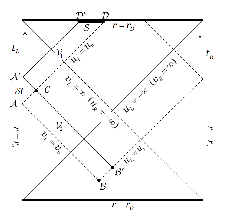
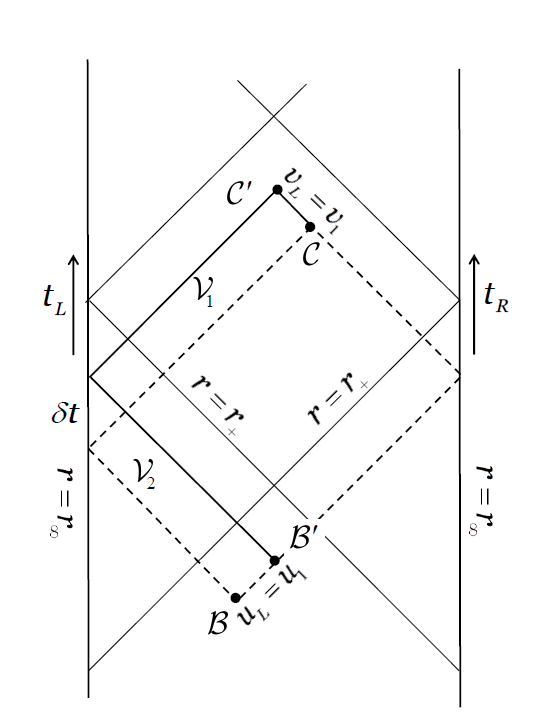
which is essentially a reproduction of Fig. 12 in [14]. Note that in this approach, each null surface has no contribution to the action due to an affine parametrization. The null joint at $r=r_{\infty}$ has a contribution to the action $S(t_{0}+\delta t)$, which is simply equal to the contribution to the action $S(t_{0})$ due to the time translation. The same holds for the joints linking the incoming null segment to the spacelike surface near the singularity at $r=2D$. This means that both joints have no contribution to the action change $\delta S$. As a result, the action change comes from the volume contributions from the regions ${\cal V}_{1}$ and ${\cal V}_{2}$, the surface contribution from the spacelike segment ${\cal S}$, and the joint contributions from the surfaces at ${\cal B^{\prime}}$ and ${\cal B}$. Namely we have

$$\delta S=S_{{\cal V}_{1}}-S_{{\cal V}_{2}}-\frac{1}{8\pi}\int_{\cal S}K\mathrm{d}\Sigma+\frac{1}{8\pi}\int_{\cal B^{\prime}}\,a\mathrm{d}S-\frac{1}{8\pi}\int_{\cal B}\,a\mathrm{d}S,$$

(15)

where $\mathrm{d}\Sigma$ is the volume element on ${\cal S}$, $\mathrm{d}S$ is the surface element on ${\cal B}^{\prime}$ and ${\cal B}$, and the integrand $a$ is given later by Eq. (22).

As in [14], we introduce two null coordinates $u_{L}$ and $v_{L}$ by $u_{L}=t_{L}+r^{*}$ and $v_{L}=t_{L}-r^{*}$ where $r^{*}=\int f^{-1}\mathrm{d}r$, where $t_{L}$ is the future-directed time on the left boundary. Note that one may similarly introduce null coordinates $u_{R}$ and $v_{R}$ with respect to the future-directed time in the right region. Since $t_{L}$ and $t_{R}$ are related analytically by $t_{R}=-t_{L}+\mathrm{const}.$, it follows that $v_{R}=-u_{L}+\mathrm{const}.$ and $u_{R}=-v_{L}+\mathrm{const}.$ in the sense of analytic continuation. Below we focus on the coordinates defined in the left region, and we omit the index $L$ from the null coordinates unless there may arise any confusion.

As shown in the left panel for Fig 1, the past and future null boundaries on the left of the first WDW patch are labeled by $u=u_{0}$ and $v=v_{0}$, respectively. These null boundaries become $u=u_{0}+\delta t$ and $v=v_{0}+\delta t$ after a time shift $\delta t$. Thus the region ${\cal V}_{1}$ is surrounded by the null surfaces $u=u_{0}$, $u=u_{0}+\delta t$, $v=v_{0}+\delta t$, and the spacelike surface ${\cal S}$ at $r=r_{D}+\epsilon$ near the singularity $r_{D}\equiv 2D$. At the end of calculations, we will take the limit $\epsilon\rightarrow 0$. The surface $v=v_{0}+\delta t$ is described by $r=\rho(u)$, where $\rho(u)$ is defined implicitly by $r^{*}(\rho)=-\frac{1}{2}(v_{0}+\delta t-u)$. Using Eq. (8), thus we have

	$\displaystyle 16\pi S_{{\cal V}_{1}}$	$\displaystyle=-\frac{4\pi}{l^{2}}\int_{u_{0}}^{u_{0}+\delta t}\mathrm{d}u\int_{r_{D}+\epsilon}^{\rho(u)}\mathrm{d}r\left(4r(r-2D)+(r-2D)^{2}+r^{2}-\frac{2Q^{2}l^{2}\mathrm{e}^{2\phi_{0}}}{r^{2}}\right)$
		$\displaystyle=-\frac{4\pi}{l^{2}}\int_{u_{0}}^{u_{0}+\delta t}\mathrm{d}u\left[2\rho(u)^{3}-6D\rho(u)^{2}+4D^{2}\rho(u)+\frac{2Q^{2}l^{2}\mathrm{e}^{2\phi_{0}}}{\rho(u)}\right]+\frac{4\pi Q^{2}\mathrm{e}^{2\phi_{0}}}{D}\delta t.$		(16)

In the second line, we have already taken the limit $\epsilon\rightarrow 0$. Note that the above volume integral has no divergence from the singularity at $r=2D$.

As shown in the left panel of Fig. 1, the region ${\cal V}_{2}$ is bounded by the null surfaces $u=u_{0}$, $u=u_{1}$, $v=v_{0}$, and $v=v_{0}+\delta t$. In this case, the volume integral in ${\cal V}_{2}$ should be done in the $(v,r)$ coordinates, where the surfaces $u=u_{0/1}$ are described by $r=\rho_{0/1}(v)$ with $r^{*}(\rho_{0/1})=-\frac{1}{2}(v-u_{0/1})$. The result turns out to be

	$\displaystyle 16\pi S_{{\cal V}_{2}}$	$\displaystyle=-\frac{4\pi}{l^{2}}\int_{v_{0}}^{v_{0}+\delta t}\mathrm{d}v\int_{\rho_{1}(v)}^{\rho_{0}(v)}\mathrm{d}r\left(4r(r-2D)+(r-2D)^{2}+r^{2}-\frac{2Q^{2}l^{2}\mathrm{e}^{2\phi_{0}}}{r^{2}}\right)$
		$\displaystyle=\left.-\frac{4\pi}{l^{2}}\int_{v_{0}}^{v_{0}+\delta t}\mathrm{d}v\left(2r^{3}-6Dr^{2}+4D^{2}r+\frac{2Q^{2}l^{2}\mathrm{e}^{2\phi_{0}}}{r}\right)\right|_{r=\rho_{1}(v)}^{r=\rho_{0}(v)}.$		(17)

After making a change of the variable $u\rightarrow u_{0}+v_{0}+\delta t-v$ in Eq. (16), the integration bound $[u_{0},u_{0}+\delta t]$ becomes $[v_{0}+\delta t,v_{0}]$, and $\rho(u)$ which satisfies $r^{*}(\rho)=-\frac{1}{2}(v_{0}+\delta t-u)\rightarrow-\frac{1}{2}(v-u_{0})$ becomes $\rho_{0}(v)$. Then combining Eq. (16) with Eq. (17), we have

$$16\pi(S_{{\cal V}_{1}}-S_{{\cal V}_{2}})=\frac{4\pi Q^{2}e^{2\phi_{0}}}{D}\delta t-\frac{4\pi}{l^{2}}\int^{v_{0}+\delta t}_{v_{0}}dv\left(2\rho^{3}_{1}-6D\rho^{2}_{1}+4D^{2}\rho_{1}+\frac{2Q^{2}l^{2}e^{2\phi_{0}}}{\rho_{1}}\right).$$

(18)

The variable $\rho_{1}(v)$ varies from $r_{\cal B}$ to $r_{\cal B^{\prime}}$ as $v$ increases from $v_{0}$ to $v_{0}+\delta t$. But the variation is small, and one has $r_{\cal B^{\prime}}=r_{\cal B}+{\cal O}(\delta t)$ so that Eq. (18) reduces to

$$16\pi(S_{{\cal V}_{1}}-S_{{\cal V}_{2}})=\frac{4\pi Q^{2}\mathrm{e}^{2\phi_{0}}}{D}\delta t-\frac{4\pi}{l^{2}}\left(2r_{\cal B}^{3}-6Dr_{\cal B}^{2}+4D^{2}r_{\cal B}+\frac{2Q^{2}l^{2}\mathrm{e}^{2\phi_{0}}}{r_{\cal B}}\right)\delta t.$$

(19)

Next we calculate the contribution from the spacelike surface ${\cal S}$ at $r=2D+\epsilon$. Its unit normal vector is given by $n_{\alpha}=|f|^{-1/2}\partial_{\alpha}r$, and the extrinsic curvature reads

$$K=\nabla_{\alpha}n^{\alpha}=\frac{1}{U^{2}}\frac{\mathrm{d}}{\mathrm{d}r}\left(U^{2}|f|^{1/2}\right),$$

(20)

and the surface element $\mathrm{d}\Sigma=4\pi|f|^{1/2}U^{2}\mathrm{d}t$. Thus the contribution from the spacelike surface has the form

$$16\pi S_{K}=-2\int_{\cal S}K\mathrm{d}\Sigma=16\pi(M-D)\delta t,$$

(21)

where we have considered the condition with $M>D$.

Finally let us calculate the contributions from the joints ${\cal B^{\prime}}$ and ${\cal B}$. Following Ref. [14], the integrand $a$ in Eq. (15) has the form

$$a=\ln(-\frac{1}{2}k\cdot\bar{k}),$$

(22)

where $k^{\alpha}$ is the future-directed null normal to the left-moving null surface, i.e., on which $v=v_{0}$ and $v=v_{0}+\delta t$, while $\bar{k}^{\alpha}$ is future-directed null normal to the right-moving surface, on which $u=u_{1}$. Under affine parametrization, they can be expressed as

$$k_{\alpha}=-c\partial_{\alpha}v=-c\partial_{\alpha}(t-r^{*}),\quad\bar{k}_{\alpha}=\bar{c}\partial_{\alpha}u=\bar{c}\partial_{\alpha}(t+r^{*}),$$

(23)

where $c$ and $\bar{c}$ are two arbitrary positive constants. This implies that one has the asymptotic normalizations $k\cdot\hat{t}_{L}=-c$ and $\bar{k}\cdot\hat{t}_{R}=-\bar{c}$, where $\hat{t}_{L,R}$ are the asymptotic Killing vectors which are normalized to describe the time flow in the left and right boundary theories, respectively. With the choice, one has $a=-\ln(-f/c\bar{c})$, and

$$16\pi S_{\cal B^{\prime}B}=2\int_{\cal B^{\prime}}a\mathrm{d}S-2\int_{\cal B}a\mathrm{d}S=8\pi[h(r_{\cal B^{\prime}})-h(r_{\cal B})],$$

(24)

where $h(r)=-U^{2}\ln(-f/c\bar{c})$. Making a Taylor expansion of $h(r)$ around $r=r_{\cal B}$ and using $r_{\cal B^{\prime}}-r_{\cal B}=-\frac{1}{2}f\delta t$, one obtains

$$16\pi S_{\cal B^{\prime}B}=\left.4\pi\delta t\left[U^{2}\frac{\mathrm{d}f}{\mathrm{d}r}+2(r-D)f\ln\left(\frac{-f}{c\bar{c}}\right)\right]\right|_{r=r_{\cal B}}.$$

(25)

Putting (19), (21), and (25) together, we have

	$\displaystyle 16\pi\frac{\mathrm{d}S}{\mathrm{d}t}$	$\displaystyle=\frac{4\pi Q^{2}\mathrm{e}^{2\phi_{0}}}{D}-\frac{4\pi}{l^{2}}\left(2r_{\cal B}^{3}-6Dr_{\cal B}^{2}+4D^{2}r_{\cal B}+\frac{2Q^{2}l^{2}\mathrm{e}^{2\phi_{0}}}{r_{\cal B}}\right)$
		$\displaystyle+16\pi(M-D)+\left.4\pi\left[U^{2}\frac{\mathrm{d}f}{\mathrm{d}r}+2(r-D)f\ln\left(\frac{-f}{c\bar{c}}\right)\right]\right|_{r=r_{\cal B}}.$		(26)

At late times, $r_{\cal B}$ approaches $r_{+}$, and $f(r)$ goes to zero. As a result, we finally arrive at

	$\displaystyle\frac{\mathrm{d}S}{\mathrm{d}t}$	$\displaystyle=2M-Q^{2}\mathrm{e}^{2\phi_{0}}\left(\frac{1}{2M}+\frac{1}{r_{+}}\right)$
		$\displaystyle=2M-\mu_{+}Q-D,\quad D=\frac{Q^{2}\mathrm{e}^{2\phi_{0}}}{2M},$		(27)

where the chemical potential $\mu_{+}=Q^{2}\mathrm{e}^{2\phi_{0}}/r$ is used. When $Q=0$, the dilaton black hole solution (11)-(14) reduces to the AdS Schwarzschild solution, while the action growth (27) goes back to the one for the AdS Schwarzschild black hole, (4), as expected. Of course, the action growth (27) is clearly different from the one for the AdS-RN black hole.

As a comparison, we now naively follow the approach proposed by Brown et al. [6, 7] to present the corresponding result for the charged dilaton black hole discussed above. In this case, the contribution from the bulk term is given by

	$\displaystyle 16\pi S_{\rm bulk}$	$\displaystyle=4\pi\delta t\int_{r_{D}}^{r_{+}}\mathrm{d}r\left(-\frac{4r(r-2D)}{l^{2}}-\frac{1}{l^{2}}((r-2D)^{2}+r^{2})+\frac{2Q^{2}\mathrm{e}^{2\phi_{0}}}{r^{2}}\right)$
		$\displaystyle=8\pi\delta t\left[-\frac{1}{l^{2}}(r_{+}^{3}-3Dr_{+}^{2}+2D^{2}r_{+})+Q^{2}\mathrm{e}^{2\phi_{0}}\left(\frac{1}{r_{D}}-\frac{1}{r_{+}}\right)\right],$		(28)

while the surface term contributes

	$\displaystyle 16\pi S_{\rm surf}$	$\displaystyle=\left.8\pi\delta tf^{1/2}\frac{\mathrm{d}(U^{2}f^{1/2})}{\mathrm{d}r}\right|^{r_{+}}_{r_{D}}$
		$\displaystyle=8\pi\delta t\left(3M-2D+\frac{1}{l^{2}}(r_{+}^{3}-3Dr_{+}^{2}+2D^{2}r_{+})-\frac{Q^{2}\mathrm{e}^{2\phi_{0}}}{r_{+}}\right).$		(29)

Combining (28) and (29), we have

$$\frac{\mathrm{d}S}{\mathrm{d}t}=2M-Q^{2}\mathrm{e}^{2\phi_{0}}\left(\frac{1}{2M}+\frac{1}{r_{+}}\right).$$

(30)

Clearly when $Q=0$, the above result does reduce to the one (4) for the AdS Schwarzschild black hole. Further it is interesting to note that Eq. (30) exactly matches the one we obtained in (27). Although these two approaches are totally different, we see that they produce the same result in this example.

In this section, we consider another example of charged black holes in AdS space, the so-called Born-Infeld black hole. The theory is described by the following action:

$$S=\frac{1}{16\pi}\int\mathrm{d}^{4}x\sqrt{-g}[R+\frac{6}{l^{2}}+{\cal L}(F)],$$

(31)

where

$${\cal L}(F)=4\beta^{2}\left(1-\sqrt{1+\frac{F_{\mu\nu}F^{\mu\nu}}{2\beta^{2}}}\right).$$

(32)

When $\beta\rightarrow\infty$, the Born-Infeld theory reduces to the Maxwell theory with ${\cal L}(F)=-F^{2}$. The Einstein field equations from the action (31) read

$$R_{\mu\nu}-\frac{1}{2}g_{\mu\nu}R-\frac{3}{l^{2}}g_{\mu\nu}=\frac{1}{2}g_{\mu\nu}{\cal L}(F)+\frac{2F_{\mu\alpha}F_{\nu}^{\,\alpha}}{\sqrt{1+F^{2}/(2\beta^{2})}}.$$

(33)

The equations of motion admit the static symmetrically symmetric black hole solution [16, 17, 18, 19]

	$\displaystyle\mathrm{d}s^{2}$	$\displaystyle=-f(r)\mathrm{d}t^{2}+f^{-1}(r)\mathrm{d}r^{2}+r^{2}\mathrm{d}\Omega^{2};$		(34)
	$\displaystyle F_{tr}$	$\displaystyle=\frac{Q}{\sqrt{r^{4}+Q^{2}/\beta^{2}}},$		(35)

where

	$\displaystyle f(r)$	$\displaystyle=1-\frac{2M}{r}+\frac{r^{2}}{l^{2}}+\frac{2\beta^{2}}{r}\int_{r}^{\infty}\mathrm{d}x\left(\sqrt{x^{4}+Q^{2}/\beta^{2}}-x^{2}\right)$
		$\displaystyle=1-\frac{2M}{r}+\frac{r^{2}}{l^{2}}+\frac{2\beta^{2}}{r}\left[I(r=\infty;a^{2}=\frac{Q^{2}}{\beta^{2}})-I(r;a^{2}=\frac{Q^{2}}{\beta^{2}})\right],$		(36)

where $I(r;a^{2})\equiv\int^{r}\mathrm{d}x\left(\sqrt{x^{4}+a^{2}}-x^{2}\right)$ is introduced for the simplicity of later computations. In the solution, $M$ and $Q$ are the mass and charge of the Born-Infeld black hole, respectively. For $r\rightarrow\infty$, $I(r;a^{2}=\frac{Q^{2}}{\beta^{2}})$ approaches a constant $I_{\infty}\equiv\frac{2}{3}a^{\frac{3}{2}}\frac{\Gamma(\frac{1}{4})\Gamma(\frac{5}{4})}{\Gamma(\frac{1}{2})}$ which depends on $Q$. Therefore in the solution the term $\beta^{2}I_{\infty}$ cannot be simply absorbed into $M$. For $r^{4}>a^{2}$, $I(r;a^{2})$ can be expressed as

$$I(r;a^{2})=I_{\infty}-\frac{r^{3}}{3}+\frac{r}{3}\sqrt{r^{4}+a^{2}}-\frac{2a^{2}}{3r}\,_{2}F_{1}[\frac{1}{4},\frac{1}{2},\frac{5}{4},-\frac{a^{2}}{r^{4}}],$$

(37)

which can be analytically continued into $r^{4}<a^{2}$ as

$$I(r;a^{2})=-\frac{r^{3}}{3}+\frac{r}{3}\sqrt{r^{4}+a^{2}}+\frac{2}{3}r\sqrt{a^{2}}\,_{2}F_{1}[\frac{1}{4},\frac{1}{2},\frac{5}{4},-\frac{r^{4}}{a^{2}}].$$

(38)

Here note that the hypergeometric function $\,{}_{2}F_{1}[a,b,c,z]$ is convergent for $|z|<1$. For $r\rightarrow 0$, we have $I(r;a^{2})\rightarrow 0$. By formally writing $I(r;a^{2})=-\frac{r^{3}}{3}+\frac{r}{3}\sqrt{r^{4}+a^{2}}+\frac{2}{3}F(r;a^{2})$, where $F^{\prime}(r;a^{2})=a^{2}/\sqrt{r^{4}+a^{2}}$, the chemical potential can be calculated as

	$\displaystyle\mu(r)Q$	$\displaystyle=\int_{r}^{\infty}\frac{Q^{2}\mathrm{d}x}{\sqrt{x^{4}+Q^{2}/\beta^{2}}}=\beta^{2}\left.F(r;\frac{Q^{2}}{\beta^{2}})\right|_{r}^{\infty}$
		$\displaystyle=\frac{Q^{2}}{r}\,_{2}F_{1}[\frac{1}{4},\frac{1}{2},\frac{5}{4},-\frac{Q^{2}}{\beta^{2}r^{4}}],$		(39)

where in the second line we have used the relation obtained from the analytic continuation,

$$F(r;a^{2})=\frac{3}{2}I_{\infty}-\frac{a^{2}}{r}\,_{2}F_{1}[\frac{1}{4},\frac{1}{2},\frac{5}{4},-\frac{a^{2}}{r^{4}}].$$

(40)

In a generic case, the Born-Infeld black hole (34)-(36) has two horizons, an outer horizon $r_{+}$ and an inner horizon $r_{-}$. Both of them satisfy the equation $f(r)=0$. The outer horizon $r_{+}$ is the large positive root of the equation $f(r)|_{r=r_{+}}=0$. And the associated temperature is given by

$$T=\frac{1}{4\pi r_{+}}\left[1+\frac{3r_{+}^{2}}{l^{2}}+2\beta^{2}r_{+}^{2}\left(1-\sqrt{1+\frac{Q^{2}}{\beta^{2}r_{+}^{4}}}\right)\right].$$

(41)

An extremal black hole corresponds to a zero temperature black hole with $T=0$. Solving the equation $T=0$, one has

$$r_{+}^{2}=\frac{l^{2}}{6}\frac{1+\frac{3}{2\beta^{2}l^{2}}}{1+\frac{3}{4\beta^{2}l^{2}}}\left(-1\pm\sqrt{1+\left(\beta^{2}Q^{2}-\frac{1}{4}\right)\frac{12\left(1+\frac{3}{4\beta^{2}l^{2}}\right)}{\beta^{2}l^{2}\left(1+\frac{3}{2\beta^{2}l^{2}}\right)^{2}}}\right).$$

(42)

We see that for the branch with sign “$-$” there is no real positive root, while for the branch with sign “ $+$,” only when $\beta^{2}Q^{2}\geq 1/4$, one has a real positive root. This indicates that only when $\beta^{2}Q^{2}\geq 1/4$ can the black hole solution have two horizons, and an extremal black hole can be achieved, while when $\beta^{2}Q^{2}<1/4$, the black hole has only one horizon and the inner horizon is absent. In other words, when $\beta^{2}Q^{2}\geq 1/4$, the Penrose diagram of the Born-Infeld black hole in AdS space is similar to the one for the AdS-RN black hole, while when $\beta^{2}Q^{2}<1/4$, the Penrose diagram is similar to the one for the AdS Schwarzschild black hole, although the Born-Infeld black hole is still charged. Now we are interested in seeing what the difference of the action growth of a WDW patch is in these two cases.