A new cosine series antialiasing function and its application to
aliasing-free glottal source models for speech and singing synthesisThanks: The main body of this article is accepted for publication in Interspeech2017.
This article has supplemental materials for details which were dropped due to limited space.
Abstract
We formulated and implemented a procedure to generate aliasing-free excitation source signals. It uses a new antialiasing filter in the continuous time domain followed by an IIR digital filter for response equalization. We introduced a cosine-series-based general design procedure for the new antialiasing function. We applied this new procedure to implement the antialiased Fujisaki–Ljungqvist model. We also applied it to revise our previous implementation of the antialiased Fant–Liljencrants model. A combination of these signals and a lattice implementation of the time varying vocal tract model provides a reliable and flexible basis to test extractors and source aperiodicity analysis methods. MATLAB implementations of these antialiased excitation source models are available as part of our open source tools for speech science.
Hideki Kawahara1, Ken-Ichi Sakakibara2, Masanori Morise3, Hideki Banno4, Tomoki Toda5
Toshio Irino1
1Wakayama University, Japan
2Health Science University of Hokkaido, Japan
3Graduate School of Science and Technology, Meijo University, Japan
4Interdisciplinary Graduate School of Medicine and Engineering, University of Yamanashi, Japan
5Graduate School of Information Science, Nagoya University, Japan
kawahara@sys.wakayama-u.ac.jp, kis@hoku-iryo-u.ac.jp, banno@meijo-u.ac.jp, mmorise@yamanashi.ac.jp, tomoki@icts.nagoya-u.ac.jp, irino@sys.wakayama-u.ac.jp
Index Terms: antialiasing, glottal source, piece-wise polynomial, piece-wise exponential, cosine series
1 Introduction
Voice quality plays important roles in speech communication, especially in para- and non-linguistic aspects. To test such aspects of speech communication, it is important to use relevant test stimuli that sound natural to listeners and that at the same time have to be precisely determined and controlled. In addition, it is desirable for the stimuli to be easy to interpret in terms of voice production, as well as auditory perception.
Source filter models with source filter interaction[1] and glottal excitation models[2, 3, 4, 5, 6, 7, 8, 9] may provide practical and useful tools. However, because glottal excitation comprises several types of discontinuity, aliasing introduces spurious signals that interfere with reliable subjective tests. This paper introduces a systematic procedure to eliminate the aliasing problem by deriving a closed form representation of the antialiased excitation. We also introduce a new set of antialiasing functions using a cosine series to keep the level of spurious signals around the Nyquist frequency low. We will make them accessible by providing MATLAB implementations as well as interactive GUI-based tools[10].
2 Background and related work
One of the authors has been developing a speech analysis, modification and resynthesis framework and related tools[11, 12, 13]. They are based on 11 1 We use “” instead of “F0” based on Reference[14]. -adaptive procedures, which require reliable and precise extraction of and aperiodicity information. Development of such extractors requires dependable ground truth. The aliasing-free L–F model (Fant–Liljencrants model) provided the ground truth for developing our new source information analysis framework[15].
A search for aliasing-free glottal source models produced one reference[16], which is not directly applicable to antialiasing of the L–F model for two reasons. First, it provides a procedure to antialias a piece-wise polynomial function, whereas the L–F model is a piece-wise exponential function. We had to derive the closed-form representation of the antialiased L–F model by ourselves[17]. Second, the reference by Milenkovic[16] had some typos, some equations were missing and a sample implementation was not available. In this article, we repaired the procedure and developed executable MATLAB functions. Retrospectively we found BLIT (band-limited impulse train)-based methods[18, 19].We found that literatures on digital representation of analog musical signals also provide aliasing reduction methods[20, 21, 22]. Our formulation with a new cosine series is more flexible and provides better aliasing suppression.
There are two important reasons for deriving an aliasing-free Fujisaki–Ljungqvist model. First reason is the relevance of the model. We found that the L–F model does not necessarily model the actual glottal source behavior, especially extreme voices[23]. Such voices sometimes consist of stronger discontinuities than the L–F model provides. The Fujisaki–Ljungqvist model provides several different levels of discontinuity and is reported to fit actual speech samples better[6].
The second and the most important reason is that it enables to develop a general procedure for antialiasing glottal source models. The Fujisaki–Ljungqvist model is a piece-wise polynomial, whereas the L–F model is a piece-wise exponential. The other popular glottal source models can be represented using both or one of these representations[2, 3, 4, 5, 6, 7, 8, 9]. Developing a procedure to make the Fujisaki–Ljungqvist model aliasing-free provides the necessary means of attaining this goal.
3 Fujisaki–Ljungqvist model
The excitation signal of the Fujisaki–Ljungqvist model is defined by the following equation in the continuous time domain[5, 6]:
where
| (7) |

Figure 1 shows the Fujisaki–Ljungqvist model parameters and waveforms. The excitation signal is a time derivative of the glottal flow . When the fundamental period is normalized to one, six model parameters determine the shape. They are and .
The Fujisaki–Ljungqvist model is a piece-wise polynomial function. Because filtering for antialiasing is a linear operation, antialiasing of the Fujisaki–Ljungqvist model is solved by adding each antialiased polynomial pulse , which is defined in using relevant scaling:
| (8) |
where the scaling is given by .
4 Antialiasing a polynomial pulse
We use the framework proposed by reference[16]22 2 Note that we removed the model weighting coefficient in the original reference[16]. It significantly simplifies the following discussion. . It starts from a matrix representation by introducing step functions and antialiasing in the continuous time domain, followed by equalization in the discrete time domain. The simplification and this equalization, as well as their application to the Fujisaki–Ljungqvist model, are our contribution.
This section fixes typos, adds missing equations and clarifies and adds missing conditions in the original reference[16]. All equations are defined in the continuous time domain.
4.1 Matrix form
Let us start with the introduction of the two step functions and , which yields
| (9) |
where is a lower triangular matrix defined as follows:
where the coefficient is a binomial coefficient, and , , and are vectors defined as follows:
4.2 Antialiasing using a cosine series
The antialiased filtered pulse has the following form:
| (26) |
where represents the convolution of and . Convolution is a linear operation and yields the following:
| (27) |
where and represent the following vectors:
Equation 27 provides the antialiased signal to be discretized. We use the following cosine series for antialiasing the filter response :
| (36) |
where represents the exponent of the highest order term and represents the length of the filter, which is determined according to the sampling frequency.
Assigning specific values to the coefficients determines and . We derive the closed-form representation of Equation 26 and then discretize it. Equations 4.2 and 40 determine and , respectively. The next step is to determine the matrices , and , with constant coefficients.
| (40) |
where each element of the vectors , , , and is defined as follows, where represents the -th element of :
| (41) |
and vectors , , and are defined thus:
| (42) |
4.3 Recursive determination of coefficients
The recursion uses the following continuity constraints and initial values. The continuity gives the following:
| (43) | |||||
| (44) |
The initial condition is for the first row of the matrices, where represents the highest exponent of the selected cosine series antialiasing function. In the following equation, represents the element of the -th row and -th column:
4.4 Closed form representation
The following equation provides the antialiased polynomial value at a given :
| where | |||
where represents logical AND. Note that we have to refine the conditions given in Reference[16] to make this procedure to work properly. The coefficient vectors are defined as follows:
5 Antialiasing function
We introduce two new cosine series antialiasing functions here. Because of the infinite frequency range of the glottal excitation models, which have discontinuities, commonly used time windowing functions with 6 dB/oct sidelobe decay[24, 25, 26, 27] introduce significant spurious due to aliasing. In our previous derivation, we used one of Nuttall’s windows[28] for the antialiasing function. The maximum side lobe level of the window is dB and the decay speed of side lobes is 30 dB/oct. This decay rate is not steep enough to suppress spurious components around , and the sidelobe level is not low enough to suppress spurious components around the Nyquist frequency. The other windows listed in [28] cannot solve both issues at the same time.
5.1 Design procedure
Using s similar process as that used in [28], we design a new set of windows to satisfy both the sidelobe level and the decay conditions. We use a cosine series to design the antialiasing function. The elements of the cosine series have the following form:
For the designed function to behave properly for antialiasing, the following conditions have to be satisfied. Note that the odd ordered derivatives are always zero for .
- Sum of coefficients should be one
-
This determines the height of the function at the origin. For simplicity, we set it to one.
- Level at the end point should be zero
-
The function should be continuous at the end point.
- Derivatives at the end point should be zero
-
Depending on the required slope, the derivatives at the end point have to be equal to zero. For the decay rate dB/oct, derivatives up to the order are zero.
These conditions are summarized by the following equations.
| (70) | ||||
| (71) | ||||
| (72) |
Once the desired decay is decided, it provides conditions. If the number of coefficients of the cosine series is equal to , there is no room for adjustment. By adding one adjustable coefficient , we can control the sidelobe level. It yields the following equation:
| (73) |
where
| (82) |
The solution is given by
| (83) |
where the elements of provide the coefficients of the cosine series. Designing an antialiasing function means tuning the parameter to minimize the target cost. This time the target is the level of the maximum sidelobe level. For a 42 dB/oct decay, a five-term cosine series is designed. For a 54 dB/oct decay, a six-term cosine series is designed.
Numerical optimization yielded the following coefficients:33 3 The coefficients are rounded to ten digits to the right of the decimal point. The best coefficients were selected from rounded numbers.
| (84) | ||||
| (85) |
Substituting these coefficients in Eq. 4.4 provides an antialiased Fujisaki–Ljungqvist model. Half of the window length is set to make the first zero of the frequency domain representation coincide with half of the sampling frequency .

Figure 2 shows the gain of these new functions and the Nuttall window that was used for the aliasing-free L–F model[17]. The five-term function has a dB maximum sidelobe level with a 42 dB/oct decay. The six-term function has a dB maximum sidelobe level with a 54 dB/oct decay. We decided to use the six-term function afterward.
5.2 Discrete time domain: equalization
The final stage, which is processed in the discrete time domain, is equalization.
The designed antialiasing functions introduce severe attenuation around the Nyquist frequency. In our antialiased L–F model, an FIR equalizer was designed to compensate for this attenuation[17]. We used a simple IIR filter with six poles in this Fujisaki–Ljungqvist model and found that it equalizes this attenuation effectively. A sample implementation produces equalized gain deviations from the FIR version within dB from 0 to 16 kHz for 44100 Hz sampling.
6 Application to glottal source models
The antialiased Fujisaki–Ljungqvist model output is obtained by the calculation of each antialiased polynomial and sum together. Discretization is the calculation of the antialiased Fujisaki–Ljungqvist model value at each sampling instance. Finally, applying the discrete time IIR equalizer to the discretized samples provides the discrete signal of the antialiased Fujisaki–Ljungqvist model.
6.1 Examples: Fujisaki–Ljungqvist model performance

We implemented this procedure using MATLAB and prepared high-level APIs. One function generates an excitation source signal using the given trajectory and the time-varying Fujisaki–Ljungqvist model parameter set and .
Figure 3 shows the power spectra of the Fujisaki–Ljungqvist model outputs. Direct discretization generates aliasing noise around dB from the peak harmonics level. The noise level of the final equalization around the fundamental component is about dB when using the six-term proposed function. Antialiasing using the Nuttall-11 window introduces approximately 20 dB higher spurious levels. (Note that the noise level using nuttallwin of MATLAB as antialiasing is approximately dB. )
6.2 Revision of antialiased L–F model
We revised our previous antialiased L–F model[17] using the new six-term cosine series and the six-pole IIR equalizer. We also reformulated the algorithm using the element function as a building block to define the antialiased and normalized complex exponential pulse :
| (86) |
where is given by Eq. 85. The factor is for the gain normalization. For each , the explicit form is as follows:
| (87) | ||||
| (88) | ||||
| (89) |
where . The functions , , and are defined in , , and ,respectively. They are 0 outside. Note that the second interval overlaps with the third one. The constant can be a complex number depending on the piece. For example, the first piece of the L–F model, is a complex number, and provides the antialiased result. For , the zeroth-order antialiased polynomial pulse is applicable.
We conducted a set of tests using this revised L-F model. Similar to Fig. 3, the noise level around the fundamental component was about dB from the peak harmonics level. This revised model is also available as a set of open access MATLAB functions.
7 Conclusions
We formulated and implemented a procedure to generate aliasing-free glottal source model output. We antialiased the Fujisaki–Ljungqvist model using a newly designed cosine series antialiasing function, followed by an IIR digital equalizer. We also revised our antialiased L–F model using the six-term cosine series and the IIR equalizer. The proposed procedure is general enough to be applicable to other glottal source models and any signal models consisting of polynomial and complex exponential segments. These antialiased models are available as open access MATALB procedures with interactive GUI tools for education and research in speech science[10]. The antialiased glottal excitation signals also provide a reliable and flexible means to test extractors and source aperiodicity analysis procedures.
8 Acknowledgments
This work was supported by JSPS KAKENHI Grant Numbers JP15H03207, JP15H02726 and JP16K12464.
References
- [1] I. R. Titze, “Nonlinear source–filter coupling in phonation: Theory,” The Journal of the Acoustical Society of America, vol. 123, no. 5, pp. 2733–2749, May 2008.
- [2] A. E. Rosenberg, “Effect of glottal pulse shape on the quality of natural vowels,” The Journal of the Acoustical Society of America, vol. 49, no. 2B, pp. 583–590, 1971.
- [3] P. Hedelin, “A glottal LPC-vocoder,” in IEEE International Conference on Acoustics Speech and Signal Processing (ICASSP), vol. 9. IEEE, 1984, pp. 21–24.
- [4] G. Fant, J. Liljencrants, and Q.-g. Lin, “A four-parameter model of glottal flow,” STL-QPSR, vol. 4, no. 1985, pp. 1–13, 1985.
- [5] H. Fujisaki and M. Ljungqvist, “Proposal and evaluation of models for the glottal source waveform,” in IEEE International Conference on Acoustics Speech and Signal Processing (ICASSP). Tokyo: IEEE, 1986, pp. 1605–1608.
- [6] ——, “Estimation of voice source and vocal tract parameters based on ARMA analysis and a model for the glottal source waveform,” in IEEE International Conference on Acoustics Speech and Signal Processing (ICASSP). IEEE, 1987, pp. 637–640.
- [7] D. H. Klatt and L. C. Klatt, “Analysis, synthesis, and perception of voice quality variations among female and male talkers.” The Journal of the Acoustical Society of America, vol. 87, no. 2, pp. 820–857, 1990.
- [8] Y.-L. Shue and A. Alwan, “A new voice source model based on high-speed imaging and its application to voice source estimation,” in IEEE International Conference on Acoustics Speech and Signal Processing (ICASSP). IEEE, 2010, pp. 5134–5137.
- [9] P. Alku, “Glottal inverse filtering analysis of human voice production - A review of estimation and parameterization methods of the glottal excitation and their applications,” Sadhana – Academy Proceedings in Engineering Sciences, vol. 36, no. October, pp. 623–650, 2011.
- [10] H. Kawahara, “SparkNG: Interactive MATLAB tools for introduction to speech production, perception and processing fundamentals and application of the aliasing-free L-F model component,” in Interspeech 2016, San Francisco, 2016. [Online]. Available: http://www.wakayama-u.ac.jp/%7ekawahara/SparkNG/
- [11] H. Kawahara, I. Masuda-Katsuse, and A. de Cheveigné, “Restructuring speech representations using a pitch-adaptive time-frequency smoothing and an instantaneous-frequency-based F0 extraction,” Speech Communication, vol. 27, no. 3-4, pp. 187–207, 1999.
- [12] H. Kawahara, M. Morise, T. Takahashi, R. Nisimura, T. Irino, and H. Banno, “TANDEM-STRAIGHT: A temporally stable power spectral representation for periodic signals and applications to interference-free spectrum, F0 and aperiodicity estimation,” in IEEE International Conference on Acoustics Speech and Signal Processing (ICASSP). Las Vegas: IEEE, 2008, pp. 3933–3936.
- [13] H. Kawahara, M. Morise, Banno, and V. G. Skuk, “Temporally variable multi-aspect N-way morphing based on interference-free speech representations,” in ASPIPA ASC 2013, 2013, p. 0S28.02.
- [14] I. R. Titze, R. J. Baken, K. W. Bozeman, S. Granqvist, N. Henrich, C. T. Herbst, D. M. Howard, E. J. Hunter, D. Kaelin, R. D. Kent, J. Kreiman, M. Kob, A. Löfqvist, S. McCoy, D. G. Miller, H. Noé, R. C. Scherer, J. R. Smith, B. H. Story, J. G. Švec, S. Ternström, and J. Wolfe, “Toward a consensus on symbolic notation of harmonics, resonances, and formants in vocalization,” The Journal of the Acoustical Society of America, vol. 137, no. 5, pp. 3005–3007, 2015.
- [15] H. Kawahara, Y. Agiomyrgiannakis, and H. Zen, “Using instantaneous frequency and aperiodicity detection to estimate F0 for high-quality speech synthesis,” arXiv preprint arXiv:1605.07809, 2016. [Online]. Available: http://arxiv.org/abs/1605.07809
- [16] P. H. Milenkovic, “Voice source model for continuous control of pitch period,” The Journal of the Acoustical Society of America, vol. 93, no. 2, pp. 1087–1096, 1993.
- [17] H. Kawahara, K.-I. Sakakibara, H. Banno, M. Morise, T. Toda, and T. Irino, “Aliasing-free implementation of discrete-time glottal source models and their applications to speech synthesis and F0 extractor evaluation,” in 2015 Asia-Pacific Signal and Information Processing Association Annual Summit and Conference (APSIPA). Hong Kong: IEEE, Dec 2015, pp. 520–529.
- [18] T. Stilson and J. Smith, “Alias-free digital synthesis of classic analog waveforms,” in Proceedings of the International Computer Music Conference, 1996, pp. 332–335.
- [19] V. Välimäki and A. Huovilainen, “Antialiasing oscillators in subtractive synthesis,” IEEE Signal Processing Magazine, vol. 24, no. 2, pp. 116–125, 2007.
- [20] V. Välimäki, J. Pakarinen, C. Erkut, and M. Karjalainen, “Antialiasing oscillators in subtractive synthesis,” Reports on Progress in Physics, vol. 69, no. 1, 2005.
- [21] V. Välimäki, “Discrete-time synthesis of the sawtooth waveform with reduced aliasing,” IEEE Signal Processing Letters, vol. 12, no. 3, pp. 214–217, March 2005.
- [22] J. Pekonen and V. Välimäki, “The brief history of virtual analog synthesis,” in Proc. 6th Forum Acusticum. Aalborg, Denmark: European Acoustics Association, 2011, pp. 461–466.
- [23] K.-I. Sakakibara, H. Imagawa, H. Yokonishi, M. Kimura, and N. Tayama, “Physiological observations and synthesis of subharmonic voices,” in Asia-Pacific Signal and Information Processing Association Annual Summit and Conference, 2011, pp. 1079–1085.
- [24] D. Slepian and H. O. Pollak, “Prolate spheroidal wave functions, Fourier analysis and uncertainty-I,” Bell System Technical Journal, vol. 40, no. 1, pp. 43–63, 1961.
- [25] D. Slepian, “Prolate spheroidal wave functions, Fourier analysis, and uncertainty-V: The discrete case,” Bell System Technical Journal, vol. 57, no. 5, pp. 1371–1430, 1978.
- [26] F. J. Harris, “On the use of windows for harmonic analysis with the discrete Fourier transform,” Proceedings of the IEEE, vol. 66, no. 1, pp. 51–83, 1978.
- [27] J. Kaiser and R. W. Schafer, “On the use of the I_0-sinh window for spectrum analysis,” IEEE Transactions on Acoustics, Speech and Signal Processing, vol. 28, no. 1, pp. 105–107, 1980.
- [28] A. H. Nuttall, “Some windows with very good sidelobe behavior,” IEEE Transactions on Audio Speech and Signal Processing, vol. 29, no. 1, pp. 84–91, 1981.
- [29] D. G. Childers and C. Ahn, “Modeling the glottal volume-velocity waveform for three voice types,” The Journal of the Acoustical Society of America, vol. 97, no. 1, pp. 505–519, 1995.
Appendix A Supplement
The main text was accepted for publication in Proc. of Interspeech2017. This appendix provides materials that were dropped owing to paucity of space.
A.1 Test signals
We used the frequency-modulated trajectory for generating the figures shown in this article. The following equation provides the details:
| (90) |
where determines the depth of the vibrato in terms of the musical cent, and determines the rate of the vibrato. We used (cent) and (Hz) to generate the figures. The Fujisaki–Ljungqvist model parameters were set as follows:
| (91) |
We also generated test signals using the antialiased L–F model. The same frequency-modulated trajectory was used. The L–F model parameters were set as follows:
| (92) |
where the specific values are the average value of the modal voices reported in Reference[29].
A.2 Spectrogram of Fujisaki–Ljungqvist model


Figure 4 shows the spectrogram of the generated excitation source signals using direct discretization, the Nuttall-11 window, and the proposed six-term cosine series. The spectrum slices in Fig. 3 are sampled from these spectrograms.
We used a self-convolved version of a Nuttall’s window for calculating these spectrograms. It is the 12th item of Table II of Reference[28]. This self-convolved window has the maximum sidelobe level at dB and a 36 dB/oct decay rate. The low sidelobe level and the steep decay rate of this window allow us to inspect low-level spurious of the proposed procedure. The window length and frame shift were 40 ms and 2 ms, respectively.
A.3 IIR equalizer design
The target equalizer shape is designed to equalize attenuation up to 68 dB for six-term and 58 dB for five-term cosine series, respectively. The FFT buffer length was 32,768, and the length of the FIR response was 161 taps. The original equalizer shape, represented as an absolute spectrum, was converted to the FIR response and truncated using one of the Nuttall windows[28]. The 12th item of Table II of the reference was used. It has a maximum sidelobe level of dB and a decay rate of 18 dB/oct.
The IIR equalizer was designed using the autocorrelation coefficients of this truncated FIR response, by applying LPC analysis.


Figure 5 shows the frequency response of each equalizer and the pole locations. The poles are not close to the unit circle, indicating the numerical stability of the equalizers.
A.4 MATLAB functions
The following MATLAB functions are prepared to generate the excitation source signals.
- antiAliasedPolynomialSegmentR
-
Generate a time normalized segment of an antialiased polynomial pulse.
- antialiasedFLmodelSingleR
-
Generate one cycle of an antialiased F-L model excitation signal.
- AAFjLjmodelFromTrajectoryR
-
Generate an antialiased F-L model excitation signal using the given trajectory and constant F-L model parameters.
- AAFjLjmodelFromTrajectoryTVR
-
Generate an antialiased F-L model excitation signal using the given trajectory and time varying F-L model parameters.
We used AAFjLjmodelFromTrajectoryR to generate the test signal used to draw Figs. 3 and 4.

Figure 6 shows an example of an excitation signal with time varying Fujisaki–Ljungqvist model parameters. The total airflow of each pitch cycle is kept constant.
A.5 Application to aliasing-free L–F model
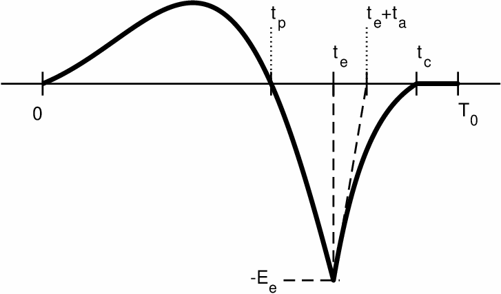
Figure 7 shows the L–F model waveform with time parameters to define it. There is a typo in the L–F model definition given on page 6 of the original reference[4], while other descriptions in the reference are correct. The fixed equation that defines the L-F model is as follows:
| (93) | |||||
| (94) |
where is defined as the time derivative of the glottal airflow . It is convenient to normalize the time axis by and the amplitude by without loss of generality. The coefficients that can then be determined from the design parameters are , and . Because the airflow is zero while the vocal fold is closed, the following constraint holds:
| (95) |
The following steps provide the parameter values. First, substitute in Eq. 94. Solving it yields . Then, use Eq. 95 and to determine . We used the numerical optimization function fzero of MATLAB to implement these steps.
A.5.1 Spectrum slice and spectrogram

