GNSS Signal Authentication via Power and Distortion Monitoring

Consider the following generic representation of an authentic GNSS signal exiting a receiver’s radio frequency (RF) front-end downconversion chain. For notational compactness, the signal is expressed by its complex baseband representation,

where $t$ is time in seconds, $P_{\rm A}$ is the received power of the authentic signal in Watts, $D(t)$ is the $\pm 1$-valued navigation data modulation, $C_{r}(t)$ is the $\pm 1$-valued pseudorandom spreading (ranging) code, $\tau_{\rm A}$ is the code phase in seconds, and $\exp(j\theta_{\rm A})$ is the carrier with phase $\theta_{\rm A}$ in radians. $P_{\rm A}$, $\tau_{\rm A}$, and $\theta_{\rm A}$ are assumed to vary with time; their time dependency is suppressed for notational simplicity. Without loss of generality for the purposes of this paper, the navigation data modulation $D(t)$ can be ignored; hence, hereafter we assume $D(t)=1$.

Let $r_{\rm I}(t)$ represent a single complex-valued interference signal that is structurally identical to $r_{\rm A}(t)$. This could be a multipath, spoofing, or jamming signal. If multipath, $r_{\rm I}(t)$ represents the strongest reflection at time $t$, whose effect on received power and correlation function distortion is a good proxy for that of the aggregate multipath. If jamming, $r_{\rm I}(t)$ represents structured-signal jamming, an especially potent form of jamming similar to spoofing except there is no expected correlation between the jamming signal’s code or carrier phase and those of $r_{\rm A}(t)$ [31]. The interference signal is modeled as

where $\eta=P_{\rm I}/P_{\rm A}$ is the interference signal’s power advantage relative to the authentic signal, and $\tau_{\rm I}$ and $\theta_{\rm I}$ are the interference signal’s code and carrier phase, respectively.

To complete the received signal model, let

be a white zero-mean complex-valued Gaussian process that models the sum of thermal noise $N(t)$, with constant spectral density $N_{0}$, and multi-access interference $M(t)$, with variable spectral density $M_{0}$. The two noise components are assumed to be independent so that $r_{\rm N}(t)$ has density $N_{0}+M_{0}$. $M(t)$ accounts for the noise contribution from other legitimate GNSS signals besides the desired signal (collectively called multi-access signals), and any interference accompanying these. With the addition of $r_{\rm N}(t)$, the full received signal-plus-interference-and-noise model is given by

As shown in Fig. 1, an AGC circuit is assumed to apply a scaling factor $\beta(t)$ to $r(t)$ so that the power in the scaled signal $\beta(t)r(t)$ remains constant. Subsequent to AGC scaling, the signal is quantized and encoded; for simplicity, these operations are ignored in Fig. 1 and in the remainder of this paper, as their effects on the this paper’s detection processing are negligible.

At the core of GNSS signal processing is correlation of $\beta(t)r(t)$ with a local replica

where $\tau$ is an arbitrary code phase lag in seconds and $C_{\ell}(t)$ is the local code replica, which, ignoring the effects of band-limiting on the received signal, is often made equal to $C_{r}(t)$. The goal of a receiver’s code and carrier tracking loops is to drive the estimates $\hat{\tau}$ and $\hat{\theta}$ to match $\tau_{\rm A}$ and $\theta_{\rm A}$ as accurately as possible. In practice, however, $\hat{\tau}$ and $\hat{\theta}$ track the code and carrier phase of the composite signal $r(t)$, not just those of $r_{\rm A}(t)$.

Correlation and accumulation over an interval $T$ ending at time $t_{k}=kT$, $k\in\{1,2,...\}$ produce the complex-valued accumulation product $\xi_{k}$, which, when viewed as a function of the arbitrary lag $\tau$ introduced by the local replica $\ell(t,\tau)$, is called the receiver’s correlation function for signal $r_{\rm A}(t)$ at time $t_{k}$, and is modeled as [32]

where $\beta_{k}$ is the average value of $\beta(t)$ over the $k$th accumulation interval, and $\xi_{{\rm A}k}(\tau)$, $\xi_{{\rm I}k}(\tau)$, $\xi_{{\rm N}k}(\tau)$ are the complex correlation function components corresponding to the authentic signal, the interference signal, and thermal noise, respectively. Fig. 2 illustrates such a correlation function.

The function $R(\tau)=E[C_{r}(t)C_{\ell}(t-\tau)]$, often called the autocorrelation function of $C_{r}(t)$ even though, strictly speaking, $C_{\ell}(t)$ may be slightly different from $C_{r}(t)$, approximates the interaction between $C_{r}(t)$ and $C_{\ell}(t)$ over the correlation and accumulation operations:

The correlation components $\xi_{{\rm A}k}(\tau)$ and $\xi_{{\rm I}k}(\tau)$ can be modeled in terms of $R(\tau)$ as

where $P_{{\rm A}k}$ and $\eta_{k}$ are the average values of $P_{{\rm A}}$ and $\eta$ over the accumulation interval, and $\Delta\tau_{{\rm A}k}$ is the average value of the difference $\tau_{\rm A}-\hat{\tau}$ over the accumulation interval, with similar definitions for $\Delta\tau_{{\rm I}k}$, $\Delta\theta_{{\rm A}k}$, and $\Delta\theta_{{\rm I}k}$.

The thermal noise component of the correlation function, $\xi_{{\rm N}k}(\tau)$, is modeled as having independent in-phase (real) and quadrature (imaginary) components, each modeled as a zero-mean Gaussian white discrete-time process:

The chip interval of the spreading code $C_{r}(t)$, denoted $\tau_{c}$, ranges from 0.01 to 1 $\mu$s in modern GNSS signals. Due to the pseudorandom nature of $C_{r}(t)$, only samples of $\xi_{{\rm N}k}(\tau)$ within $2\tau_{c}$ of each other are correlated [33]:

Here, ^∗ denotes the complex conjugate and $\sigma_{\rm N}^{2}$ is the variance of the in-phase and quadrature components of $\xi_{{\rm N}k}(\tau)$, which is related to the spectral density of the white noise process $r_{\rm N}(t)$ by $\sigma_{\rm N}^{2}=(N_{0}+M_{0})/2T$.

In what follows, we denote the marginal distributions of $w_{i}({\theta})$ by $w_{\eta i}(x)$, $w_{\Delta\tau i}(x)$, and $w_{\Delta\theta i}(x),~i\in\mathcal{I}$. Under the null hypothesis ($i=0$), which corresponds to the interference-free case, we have

It follows that $w_{\eta 0}(x)$ is equivalent to the Dirac delta function. The marginal distributions $w_{\Delta\tau 0}(x)$, and $w_{\Delta\theta 0}(x)$ can be defined arbitrarily, since for $\eta=0$ they have no effect on $r(\delta)$.

In the case of multipath, $\eta$ and $\Delta\tau$ can be bounded as follows:

The bounds $\eta_{1}$ and $\Delta\tau_{1}$ are informed by the physics of signal reception and signal processing, as follows. Whenever the authentic signal is unobstructed, it arrives with greater power than any echo, whose additional path length and interaction with reflection surfaces invariably attenuate its power [36]. Moreover, an echo whose delay is more than double the spreading code chip interval (e.g., more than 0.2 $\mu$s for $\tau_{c}=0.1$ $\mu$s) causes no correlation function distortion [33], and, due to the additional path loss, is at least 3 dB weaker than an unobstructed authentic signal [37]. Thus, its effect on $r(\delta)$ is negligible. It follows that $\eta_{1}=1$ and $\Delta\tau_{1}=2\tau_{c}$ upper-bound the multipath parameter set for an unobstructed authentic signal.

On the other hand, the severe shadowing experienced by mobile receivers can cause $\eta>1$, especially in urban environments where surrounding buildings simultaneously attenuate and reflect authentic signals [37]. In these situations, there is no practical upper limit on $\eta$ because the direct-path authentic signal may be attenuated by 50 dB or more. It is not possible to reliably distinguish multipath from low-power spoofing in such circumstances.

One can avoid this difficulty by applying this paper’s detection test only when the authentic signal $r_{\rm A}(t)$ is received without severe shadowing, in which case the probability that $\eta>1$ under $H_{1}$ again becomes negligible. In particular, the multipath model developed below assumes that $r_{\rm A}(t)$ is attenuated less than 6 dB by shadowing. In practice, one simply excludes cases in which the received power $P_{k}$ is not unusually high yet the measured carrier-to-noise ratio $C/N_{0}$ drops by more than 6 dB from its modeled value for an unobstructed authentic signal.

An analysis of GNSS multipath was carried out to validate the bounds $\eta_{1}=1$ and $\Delta\tau_{1}=2\tau_{c}$ and to characterize $w_{1}({\theta})$. The analysis was based on the Land Mobile Satellite Channel Model (LMSCM) [38], itself based on extensive experimentation with a wideband airborne transmitter at GNSS frequencies in urban and suburban environments [37, 38]. The LMSCM generates power, delay, and carrier phase for both line-of-sight and echo signals using deterministic models for attenuation, diffraction, and delay that respond to stochastically-generated obstacles and reflectors in the simulation environment.

In keeping with the philosophy of robust detection, multipath scenarios were sought whose distribution $w_{1}({\theta})$ was most similar to the distribution for spoofing, $w_{2}({\theta})$. From the standpoint of distinguishing multipath from spoofing, this is the worst-case $w_{1}({\theta})$. As a practical matter, the worst-case $w_{1}({\theta})$ has a high proportion of large $\eta$ values and a wide range of $\Delta\theta$. Not surprisingly, urban LMSCM scenarios with low-elevation satellite signals yielded the worst-case $w_{1}({\theta})$.

For flexibility of detector design, the simulation-derived $w_{1}({\theta})$ was parameterized in terms of satellite elevation angle $\alpha_{e}$. Several 1-minute LMSCM simulations with randomly-created urban environments and various satellite azimuth angles were run for $\alpha_{e}\in[20,80]$ degrees. At each simulation epoch, the maximum-amplitude echo was identified and its relative power, delay, and phase with respect to the line-of-sight signal were taken as sampled $\eta$, $\Delta\tau$, and $\Delta\theta$ values from which $w_{1}({\theta})$ could be approximated. Epochs whose line-of-sight signal was attenuated by more than 6 dB were excluded, resulting in exclusion of up to 90% of epochs for heavily-shadowed scenarios at $\alpha_{e}=20$, but less than 1% of epochs at $\alpha_{e}=80$. At each $\alpha_{e}$, the scenario producing the worst-case $w_{1}({\theta})$ was selected.

A statistical analysis of the sampled $\eta$, $\Delta\tau$, and $\Delta\theta$ values revealed that the relative phase $\Delta\theta$ was uniformly distributed on $[0,2\pi)$ and independent of $\eta$, $\Delta\tau$, which is unsurprising given the wavelength-scale sensitivity of $\Delta\theta$ to path length. The parameters $\eta$ and $\Delta\tau$ were found to be significantly correlated, with a linear correlation coefficient of approximately $\rho=-0.23$, implying that more distant reflectors tend to produce weaker echos. Consistent with [36], the marginal distribution $w_{\eta 1}(x)$ was found to be log-normal, with a mean of $-21$ dB and a standard deviation of 5 dB, both insensitive to $\alpha_{e}$. Thus, excluding cases of heavy line-of-sight signal shadowing, multipath causes $\eta>1$ with negligible probability, which indicates that $\eta_{1}=1$ is an unproblematic bound. The marginal distribution $w_{\Delta\tau 1}(x)$ was found to be exponential,

with $\mu$ a quadratic function of $\alpha_{e}$,

where $\alpha_{e}$ is expressed in degrees and $\Delta\tau$ in nanoseconds. Thus, $\Delta\tau$ values are widely spread at low $\alpha_{e}$ but tightly clustered near zero at high $\alpha_{e}$, consistent with the empirical distributions in [37].

Under the spoofing hypothesis, we take $\eta_{1}=1$ as a lower bound for $\eta$ and assume $|\Delta\tau|$ is upper-bounded by $\Delta\tau_{1}=2\tau_{c}$:

These bounds make sense because the spoofing signal must be at least as powerful as the authentic signal for reliable spoofing, and because spoofing whose $|\Delta\tau|$ value exceeds $\Delta\tau_{1}=2\tau_{c}$ is no longer classified as carry-off-type spoofing, since the interference is uncorrelated with the authentic signal. Instead, for $|\Delta\tau|\geq\Delta\tau_{1}$, the attack is classified as jamming.

For maximum stealth, the distribution $w_{2}({\theta})$ should be as close as possible to $w_{1}({\theta})$ while respecting the bounds $\eta_{1}$ and $\Delta\tau_{1}$ and allowing a wide range of $\Delta\tau$ for code pull-off. Thus, $w_{\eta 2}(x)$ is modeled as log-normal with mean of 1 dB and standard deviation a fraction of a dB, $w_{\Delta\tau 2}(x)$ as exponential with parameter $\mu=120$ (mimicking low-elevation multipath), and $w_{\Delta\theta 2}(x)$ as uniform on $[0,2\pi)$.

Because it is uncorrelated with the authentic signal, jamming is taken to have $|\Delta\tau|\geq\Delta\tau_{1}=2\tau_{c}$. Its power advantage is assumed to be at least $\eta_{1}=1$, as weaker jamming is both harmless and so common as to be unremarkable. Thus, the jamming parameter set is

The marginal distribution $w_{\eta 3}(x)$ is taken to be Rician. By adjusting the Rician distance and scale parameters $\nu$ and $\sigma$, one can model high- or low-power jamming within a wide or narrow range. The marginal distributions $w_{\Delta\tau 3}(x)$ and $w_{\Delta\theta 3}(x)$ can be modeled arbitrarily, as they have no effect on $r(\delta)$ since $|\Delta\tau|\geq\Delta\tau_{1}$ eliminates correlation with the authentic signal.

The total received power measured by a GNSS receiver in an RF band of interest, denoted $P_{k}$ for measurement time $t_{k}$, is a simple and effective indicator of interference [39, 20]. Even subtle spoofing attacks with power advantage $\eta$ near unity can cause an increase in $P_{k}$ that is distinguishable from random variations, including so-called nulling attacks that attempt to suppress the authentic signals [31]. The catch is that routine events such as solar radio bursts and the near passage of a so-called personal privacy device can also cause $P_{k}$ to rise above nominal levels [31]. Thus, to prevent an anomalous-power monitor from issuing alarms intolerably often, the alarm threshold may need to be raised to a point where the monitor is no longer sensitive to subtle spoofing attacks. This is why power monitoring is best coupled with other forms of interference monitoring.

Suppose $M_{s}+1$ authentic signals modeled as (1) are received, each with its associated interference signal, modeled as (2). Let $r_{{\rm A}i}(t)$ and $r_{{\rm I}i}(t)$ represent the $i$th authentic and interference signals. The combined signal exiting the RF front end is then

where $N(t)$ is the same thermal noise component as in (3).

Receivers with sufficient dynamic range in the discrete samples produced from $r_{\rm C}(t)$ do not require an AGC and so can compute received power directly by averaging the squared modulus of these samples. Let $W_{P}$ be the bandwidth over which $P_{k}$ is to be measured. If $W_{P}$ is narrower than the receiver front-end’s native bandwidth, then $r_{\rm C}(t)$ must be filtered to isolate the desired spectral interval. Fig. 3 shows 2- and 8-MHz bands for $P_{k}$, with Fig. 4 showing corresponding power time histories. In a receiver whose front end is equipped with an AGC, $P_{k}$ is measured indirectly through the AGC setpoint [20]. In this case $W_{P}$ is equivalent to the front-end noise-equivalent bandwith.

Let $\tilde{r}_{\rm C}(t)$ represent the (optionally) filtered version of $r_{\rm C}(t)$ from which $P_{k}$ is to be measured. $P_{k}$ is calculated as the average power in $\tilde{r}_{\rm C}(t)$ over the interval $t_{k-1}$ to $t_{k}$:

Let $p_{P_{k}}(x|\theta)$ be the conditional density of $P_{k}$. Assuming $W_{P}$ is wide enough that $\tilde{r}_{\rm C}(t)$ retains the significant power in $r_{{\rm A}i}(t)$ and $r_{{\rm I}i}(t)$, then $p_{P_{k}}(x|\theta)$ can be modeled as Gaussian, i.e., $p_{P_{k}}(x|\theta)=\mathcal{N}(x;\bar{P}_{k},\sigma_{P}^{2})$, where $\bar{P}_{k}$ and $\sigma_{P}$ are expressed in dBW. The mean, $\bar{P}_{k}$, revealed by carrying out the multiplications inherent in $|\tilde{r}_{\rm C}(t)|^{2}=\tilde{r}_{\rm C}(t)\tilde{r}_{\rm C}^{*}(t)$, and by noting that $N(t)$ is zero-mean and independent of $r_{{\rm A}i}(t)$ and $r_{{\rm I}i}(t)$, and that, due orthogonality of spreading codes, $E[r_{{\rm A}i}(t)r_{{\rm A}i}^{*}(t)]=E[r_{{\rm I}i}(t)r_{{\rm I}l}^{*}(t)]=0$ for all $i\neq l$, is $\bar{P}_{k}=10\log_{10}(\bar{P}_{\rm L})$, where

and the subscript $i$ associates the corresponding quantity with the $i$th signal. The first term in the summation is the non-coherent sum of power in $r_{{\rm A}i}$ and $r_{{\rm I}i}$; the second term is the power contributed by coherent interaction between $r_{{\rm A}i}$ and $r_{{\rm I}i}$. If $\eta_{i}=0$, or if the interference is orthogonal to the authentic signal (e.g., $\Delta\theta_{i}=\pm\pi/2$), or if $\Delta\tau_{i}$ is large enough that $R(\Delta\tau_{i})=0$, then this second term vanishes.

The deviation $\sigma_{P}$ about $\bar{P}_{k}$ accounts for unpredictable but natural variations in $P_{k}$ such as measurement error due to the finite duration over which $P_{k}$ is estimated. From the top plot of Fig. 4, one can see that for the receiver under test, $\sigma_{P}$ is at approximately 0.1 dB and 0.05 dB, respectively, for 2- and 8-MHz bandwidths. For urban RF environments, in which significant low-level interference is present in the GNSS bands, $\sigma_{P}$ can be as high as 0.5 dB in a 2-MHz bandwidth. This paper’s detection test assumes $\sigma_{P}=0.4$ dB.

For modeling completeness, the multi-access interference $M(t)$ in (3) can be interpreted in terms of the model for $r_{\rm C}(t)$ in (7). $M(t)$ models the effect of multi-access interference for a particular desired signal, $r_{\rm A}(t)$. Invoking the so-called thermal-noise approximation [31], $M(t)$ is assumed to be spectrally flat with density $M_{0}$, whose variable value is a function of the spreading code’s chip interval, $\tau_{c}$, and of the average power $\bar{P}_{\rm M}$ and number $M_{s}$ of multi-access signals. For GNSS signals with a ${\rm sinc}^{2}(f\tau_{c})$-shaped power spectrum, which applies for all GPS signals except the new military M-code signals, $M_{0}$ is given by [31]

Three example cases for $\bar{P}_{\rm M}$ are given below. In each case, $i=0$ indicates the desired authentic signal and its interferer, whereas $i=1,...,M_{s}$ indicate multi-access signals and their interferers.

$\bar{P}_{\rm M}=P_{\rm A}$:

In this case, $P_{{\rm A}i}=P_{\rm A}$ for $i=0,...,M_{s}$ and $\eta_{i}=0$ for $i=1,...,M_{s}$. In other words, $P_{\rm A}$ is assumed to be typical of the received power from all GNSS signals and no other interference besides $r_{{\rm I}0}$ is assumed. This case applies for $H_{0}$, for $H_{1}$ when only a single signal, $r_{{\rm A}0}$, experiences significant multipath, and for $H_{2}$ when the spoofing attack targets only $r_{{\rm A}0}$, as opposed to an attack against all $r_{{\rm A}i}$.

$\bar{P}_{\rm M}=(1+\eta)P_{\rm A}$:

In this case, $P_{{\rm A}i}=P_{\rm A}$ and $\eta_{i}=\eta$ for $i=0,...,M_{s}$. In other words, each of the $M_{s}+1$ received signals is modeled as having power $P_{\rm A}$, and each is assumed to be subject to a non-coherent interferer with power $\eta P_{\rm A}$. This case applies for the jamming hypothesis $H_{3}$, as follows: For all $i$, $|\Delta\tau_{i}|$ is assumed to be large enough that $R(\Delta\tau_{i})=0$, causing the second term of the summation in (9) to vanish. Jamming power manifests in the first term of the summation as an additional $\eta_{i}P_{{\rm A}i}=\eta P_{\rm A}$.

This case also applies for $H_{2}$ when the spoofing-to-authentic phase difference $\Delta\theta_{i}$ for $i=0,...,M_{s}$ can be modeled as a random variable uniformly distributed on $[0,2\pi)$, in which case the second term of the summation in (9) vanishes for all $i$.

$\bar{P}_{\rm M}=(1+\eta)P_{\rm A}+2\sqrt{\eta}P_{\rm A}\cos(\Delta\theta)R(\Delta\tau)$:

This case applies for $H_{2}$ when the spoofing attack targets not only $r_{{\rm A}0}$ but also the $M_{s}$ multi-access signals such that $\eta_{i}P_{{\rm A}i}=\eta P_{\rm A}$, $\Delta\theta_{i}=\Delta\theta$ and $\Delta\tau_{i}=\Delta\tau$ for $i=0,...,M_{s}$.

A variety of signal quality monitoring (SQM) metrics have been applied to detect distortions in $\xi_{k}(\tau)$ caused by anomalous GNSS signals, including spoofing signals [40, 41, 42, 22, 21, 43, 44]. Among these, the so-called symmetric difference is particularly attractive for multipath and spoofing detection because it is simple to implement, is insensitive to the particular shape of the correlation function (provided the function is symmetric about $\tau=0$, as is the case for all current and proposed GNSS signals), and is sensitive to the correlation function distortion introduced by spoofing whenever the authentic and spoofing signals are approximately matched in power (i.e., $0.1<\eta<10$). Fig. 5 illustrates $\xi_{k}(\tau)$ under nominal conditions (top) and a spoofing attack (bottom).

Let $\tau_{d}$ be the offset of the early and late symmetric difference taps from $\tau=0$, and let $\sigma_{{\rm N}0}$ be the value of $\sigma_{\rm N}$ in the interference-free case, for which we assume $M_{0}$ is given by (10) with $\bar{P}_{\rm M}=P_{\rm A}$. Then at measurement time $t_{k}$ the symmetric difference is calculated as the modulus of the complex difference between the early and late symmetric difference taps, scaled by $1/\sigma_{{\rm N}0}$:

As with $P_{k}$, a statistical model for $D_{k}(\tau_{d})$ is necessary to develop a Bayesian detection framework. Let $p_{D_{k}}(x|\theta)$ denote the conditional density of $D_{k}$. An analytical model for $p_{D_{k}}(x|\theta)$ is easily derived when there is no coherent interaction between $r_{\rm A}$ and $r_{\rm I}$, that is, when the second term of the summation in (9) vanishes, which occurs in the interference-free case ($\eta=0$) or in the case of jamming, for which $R(\Delta\tau)=0$. Let $P_{H_{0}}$ denote the received power when $\eta=0$, which, as evident in the top panel of Fig. 4, is constant to within a few tenths of a dB. Assume that, for any $r(t)$ and any $k\in\{1,2,...\}$, the AGC adjusts $\beta_{k}$ such that the average power in $\beta_{k}r(t)$ over $t_{k-1}$ to $t_{k}$ is $P_{H_{0}}$. Then, if code tracking is accurate ($\Delta\tau_{{\rm A}k}\approx 0$), as would be true for up to moderate jamming, or if the amplitude of $\xi_{A}$ is small with respect to $\sigma_{\rm N}$, as would be true for strong jamming, then the scaled complex difference $[\xi_{k}(-\tau_{d})-\xi_{k}(\tau_{d})]/\sigma_{{\rm N}0}$ can be modeled as a zero-mean complex Gaussian random variable with variance

It follows that $p_{D_{k}}(x|\theta)$ in this case is Rayleigh with scale parameter $\frac{\sigma_{d}}{\sqrt{2}}$:

In the interference-free case, $\beta_{k}=1$ and $\sigma_{\rm N}=\sigma_{{\rm N}0}$, so $\sigma_{d}^{2}$ reduces to $\sigma_{d}^{2}=8\tau_{d}$. One can show that this simplified expression for $\sigma_{d}^{2}$ is also approximately true for wideband jamming, for which the AGC maintains $(\beta_{k}\sigma_{\rm N}/\sigma_{{\rm N}0})^{2}\approx 1$. However, the structured-signal jamming assumed in this paper is more potent than wideband jamming: it increases $M_{0}$, and therefore $\sigma_{\rm N}$, more than equivalently-powered wideband jamming [31]. As a result, $\sigma_{d}^{2}$ rises with increasing power of structured-signal jamming, making it more difficult to distinguish jamming from spoofing. Nevertheless, assuming structured-signal jamming, as opposed to the less potent wideband or narrowband jamming, is consonant with this paper’s focus on worst-case attacks.

Note that a version of the symmetric difference normalized by the maximum magnitude of $\xi_{k}(\tau)$ has also been proposed for SQM and spoofing detection [40, 41, 23]. But the definition of $D_{k}$ in (11) is more convenient because its distribution for $\eta=0$ depends only on $\sigma_{d}$, as evident in (13).

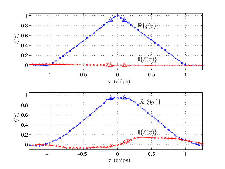
Modeling $p_{D_{k}}(x|\theta)$ as Rayleigh only holds for $\eta=0$ or $R(\Delta\tau)=0$. When neither of these conditions is true, the real and imaginary components of $\xi_{k}(\tau)$ can manifest strong asymmetry, as shown in the bottom panel of Fig. 5. In this case, the possible interactions of $\xi_{{\rm I}k}(\tau)$, and $\xi_{{\rm A}k}(\tau)$ are so complex that $p_{D_{k}}(x|\theta)$ cannot be modeled analytically. It can, however, be studied through Monte-Carlo simulation of (5) and (11) as a function of $\theta=[\eta,\Delta\tau,\Delta\theta]^{T}$ and $\tau_{d}$, together with some assumed recipe for determination of $\hat{\tau}$, the receiver’s estimate of $\tau_{\rm A}$. For this paper, we have assumed that

which holds for early-minus-late DLL tracking (both coherent and non-coherent) in the limit as $\tau_{\rm DLL}\rightarrow 0$, provided the tracking points have not settled on a local maximum different from the global maximum. Note that to minimize the number of correlation taps, one can choose $\tau_{\rm DLL}=\tau_{d}$, where $\tau_{\rm DLL}$ is the offset from $\tau=0$ of the DLL’s early and late taps. But, depending on the shape of $\xi_{k}(\tau)$ and the assumed distribution of $\tau_{\rm I}$, unequal $\tau_{\rm DLL}$ and $\tau_{d}$ may improve tracking and detection performance.

In simulation, one can apply whatever algorithm for producing $\hat{\tau}$ best approximates the operation of the receiver, or class of receivers, whose reaction to interference one wishes to simulate. For example, a multipath-mitigating receiver may estimate $\tau_{\rm A}$ by (1) assuming the presence of one or more multipath components, (2) estimating the parameters $\eta,\tau_{\rm I}$ and $\theta_{\rm I}$ for each component, and (3) subtracting a model of each component from $\xi_{k}(\tau)$ [45].

The symmetric difference for tracking channel $i\in\{1,2,...,N\}$ at time $t_{k}$, denoted $D_{k}^{i}(\tau_{d})$, can be combined with the received power measurement to form a channel-specific vector of observables at $t_{k}$:

$D_{k}^{i}(\tau_{d})$ and $P_{k}$ are modeled as independent so that

where $z_{jk}^{i}$ is the $j$th element of $z_{k}^{i}$.

Obviously, when multiple GNSS signals are simultaneously affected by interference, detection performance improves by considering the multi-channel observation vector

For clarity of presentation and analysis, the channel-specific vector ${z}_{k}^{i}$ has been taken as the observation vector for this paper’s Bayesian detection strategy, with the superscript $i$ dropped for notational simplicity. Extension of this paper’s methods to the multi-channel case follows straightforwardly from the principles of the per-channel test along with a model for correlation between the $D_{k}^{i}(\tau_{d})$.

A spoofer can minimize the hallmark distortions of an attack by generating an antipodal, or nulling, signal or by preventing reception of the authentic signal (e.g., by emplacing an obstruction). The form given for $r_{\rm I}(t)$ in (2) accommodates a nulling attack in which $r_{\rm I}(t)$ is made antipodal to $r_{\rm A}(t)$ via the following settings: $\eta=1$, $\tau_{\rm I}=\tau_{\rm A}$, and $\theta_{\rm I}=\theta_{\rm A}+\pi$. This attack annihilates $r_{\rm A}(t)$, producing an effect similar to jamming but with much less received power. But the form in (2) does not accommodate the nulling-and-replacement attack described in [6] and [31], whereby, after nulling $r_{\rm A}(t)$, the attacker supplants it with a separate spoofing signal. Detection of a perfectly-executed nulling-and-replacement attack is, in fact, not possible with the technique developed in this paper. Such an attack is, however, extremely difficult to carry out in practice, as it requires centimeter-level knowledge of, and a highly accurate fading model for, the attacker-to-receiver signal path.

Similarly, blocking reception of $r_{\rm A}(t)$ by physical obstruction is difficult in cases where the receiver antenna is not physically accessible to the attacker. The technique developed in this paper makes the assumption that a nulling-and-replacement attack is impractically difficult and that physical access to the receiving antenna is controlled to prevent signal blockage. It must be recognized, however, that in many cases of practical interest (e.g., fishing vessel monitoring), the receiver and antenna are fully under the control of potential attackers.

An alternative approach to eliminating telltale distortion is an overpowered spoofing attack in which $\eta$ is set so high that the receiver’s AGC squelches the relatively weak authentic signals below the noise floor, thereby eliminating interaction between $r_{\rm I}$ and $r_{\rm A}$. In other words, as $\eta$ increases, $\beta_{k}$ decreases to maintain a constant power in $\beta_{k}r(t)$, with the result that $\beta_{k}r_{\rm A}(t)$ becomes negligible compared to $\beta_{k}r_{\rm I}(t)$. If, however, the receiver raises an alarm when the received power $P_{k}$ exceeds some threshold, then covert spoofing is strictly limited to $\eta<\eta_{\rm max}$ for some $\eta_{\rm max}$.

The spoofer can also minimize correlation function distortion by selecting a small $\eta$. However, reliable capture of the receiver’s tracking loops requires $\eta>\eta_{\rm min}\approx 0.4~$dB [46]. Thus, for spoofing to be both reliable and covert, $\eta$ is lower bounded by $\eta_{\rm min}$ and upper bounded by $\eta_{\rm max}$.

This paper’s approach to spoofing detection can be stated as follows: If the defending receiver is designed such that $\eta_{\rm max}$ is sufficiently low despite maintaining a tolerable rate of false alarm in the received power monitor, then a carry-off spoofing attack that respects this bound yet successfully captures the receiver’s tracking loops will unavoidably and detectably distort the correlation function $\xi_{k}(\tau)$. This distortion, evident in $D_{k}(\tau_{d})$, can be distinguished from distortion due to multipath by its greater magnitude and by a concomitant increase in $P_{k}$.

References

- [1] GPS Directorate, “Systems engineering and integration Interface Specification IS-GPS-200G,” 2012, http://www.gps.gov/technical/icwg/.
- [2] European Union, “European GNSS (Galileo) open service signal in space interface control document,” 2010, http://ec.europa.eu/enterprise/policies/satnav/galileo/open-service/.
- [3] T. E. Humphreys, B. M. Ledvina, M. L. Psiaki, B. W. O’Hanlon, and P. M. Kintner, Jr., “Assessing the spoofing threat: Development of a portable GPS civilian spoofer,” in Proceedings of the ION GNSS Meeting. Savannah, GA: Institute of Navigation, 2008.
- [4] John A. Volpe National Transportation Systems Center, “Vulnerability assessment of the transportation infrastructure relying on the Global Positioning System,” 2001.
- [5] D. P. Shepard, T. E. Humphreys, and A. A. Fansler, “Evaluation of the vulnerability of phasor measurement units to GPS spoofing attacks,” International Journal of Critical Infrastructure Protection, vol. 5, no. 3-4, pp. 146–153, 2012.
- [6] M. L. Psiaki and T. E. Humphreys, “GNSS spoofing and detection,” Proceedings of the IEEE, vol. 104, no. 6, pp. 1258–1270, 2016.
- [7] K. D. Wesson, M. P. Rothlisberger, and T. E. Humphreys, “Practical cryptographic civil GPS signal authentication,” Navigation, Journal of the Institute of Navigation, vol. 59, no. 3, pp. 177–193, 2012.
- [8] T. E. Humphreys, “Detection strategy for cryptographic GNSS anti-spoofing,” IEEE Transactions on Aerospace and Electronic Systems, vol. 49, no. 2, pp. 1073–1090, 2013.
- [9] A. J. Kerns, K. D. Wesson, and T. E. Humphreys, “A blueprint for civil GPS navigation message authentication,” in Proceedings of the IEEE/ION PLANS Meeting, May 2014.
- [10] I. Fernández-Hernández, V. Rijmen, G. Seco-Granados, J. Simon, I. Rodríguez, and J. D. Calle, “A navigation message authentication proposal for the Galileo open service,” Navigation, vol. 63, no. 1, pp. 85–102, 2016.
- [11] M. Psiaki, B. O’Hanlon, J. Bhatti, D. Shepard, and T. Humphreys, “GPS spoofing detection via dual-receiver correlation of military signals,” IEEE Transactions on Aerospace and Electronic Systems, vol. 49, no. 4, pp. 2250–2267, 2013.
- [12] P. Y. Montgomergy, T. E. Humphreys, and B. M. Ledvina, “Receiver-autonomous spoofing detection: Experimental results of a multi-antenna receiver defense against a portable civil GPS spoofer,” in Proceedings of the ION International Technical Meeting, Anaheim, CA, Jan. 2009.
- [13] M. L. Psiaki, B. W. O’Hanlon, S. P. Powell, J. A. Bhatti, K. D. Wesson, and T. E. Humphreys, “GNSS spoofing detection using two-antenna differential carrier phase,” in Proceedings of the 27th Meeting of the Satellite Division of the Institute of Navigation (ION GNSS+ 2014). ION, 2014.
- [14] M. Meurer, A. Konovaltsev, M. Cuntz, and C. Hättich, “Robust joint multi-antenna spoofing detection and attitude estimation using direction assisted multiple hypotheses RAIM,” in Proceedings of the 25th Meeting of the Satellite Division of the Institute of Navigation (ION GNSS+ 2012). ION, 2012.
- [15] D. Borio, “PANOVA tests and their application to GNSS spoofing detection,” IEEE Transactions on Aerospace and Electronic Systems, vol. 49, no. 1, pp. 381–394, Jan. 2013.
- [16] M. Psiaki, S. P. Powell, and B. W. O’Hanlon, “GNSS spoofing detection using high-frequency antenna motion and carrier-phase data,” in Proceedings of the ION GNSS+ Meeting, 2013, pp. 2949–2991.
- [17] E. McMilin, D. S. De Lorenzo, T. Walter, T. H. Lee, and P. Enge, “Single antenna GPS spoof detection that is simple, static, instantaneous and backwards compatible for aerial applications,” in Proceedings of the 27th International Technical Meeting of The Satellite Division of the Institute of Navigation (ION GNSS+ 2014), Tampa, FL, 2014, pp. 2233–2242.
- [18] N. White, P. Maybeck, and S. DeVilbiss, “Detection of interference/jamming and spoofing in a DGPS-aided inertial system,” IEEE Transactions on Aerospace and Electronic Systems, vol. 34, no. 4, pp. 1208–1217, 1998.
- [19] C. Tanıl, S. Khanafseh, and B. Pervan, “GNSS spoofing attack detection using aircraft autopilot response to deceptive trajectory,” in Proceedings of the ION GNSS+ Meeting. ION, 2015.
- [20] D. M. Akos, “Who’s afraid of the spoofer? GPS/GNSS spoofing detection via automatic gain control (AGC),” Navigation, Journal of the Institute of Navigation, vol. 59, no. 4, pp. 281–290, 2012.
- [21] B. M. Ledvina, W. J. Bencze, B. Galusha, and I. Miller, “An in-line anti-spoofing module for legacy civil GPS receivers,” in Proceedings of the ION International Technical Meeting, San Diego, CA, Jan. 2010.
- [22] A. Cavaleri, B. Motella, M. Pini, and M. Fantino, “Detection of spoofed GPS signals at code and carrier tracking level,” in 5th ESA Workshop on Satellite Navigation Technologies and European Workshop on GNSS Signals and Signal Processing, Dec. 2010.
- [23] J. Huang, L. L. Presti, B. Motella, and M. Pini, “GNSS spoofing detection: Theoretical analysis and performance of the ratio test metric in open sky,” ICT Express, vol. 2, no. 1, pp. 37–40, 2016.
- [24] R. Mitch, R. Dougherty, M. Psiaki, S. Powell, B. O’Hanlon, J. Bhatti, and T. E. Humphreys, “Know your enemy: Signal characteristics of civil GPS jammers,” GPS World, Jan. 2012.
- [25] K. D. Wesson, B. L. Evans, and T. E. Humphreys, “A combined symmetric difference and power monitoring GNSS anti-spoofing technique,” in IEEE Global Conference on Signal and Information Processing, 2013.
- [26] T. E. Humphreys, J. A. Bhatti, D. P. Shepard, and K. D. Wesson, “The Texas Spoofing Test Battery: Toward a standard for evaluating GNSS signal authentication techniques,” in Proceedings of the ION GNSS Meeting, 2012, http://radionavlab.ae.utexas.edu/texbat.
- [27] T. R. Laboratory, “Texas Spoofing Test Battery (TEXBAT),” July 2017, http://radionavlab.ae.utexas.edu/texbat.
- [28] T. Humphreys, “TEXBAT data sets 7 and 8,” 2016, http://radionavlab.ae.utexas.edu/datastore/texbat/texbat_ds7_and_ds8.pdf.
- [29] K. D. Wesson, D. P. Shepard, J. A. Bhatti, and T. E. Humphreys, “An evaluation of the vestigial signal defense for civil GPS anti-spoofing,” in Proceedings of the ION GNSS Meeting, Portland, OR, 2011.
- [30] K. Pesyna, Z. Kassas, J. Bhatti, and T. Humphreys, “Tightly-coupled opportunistic navigation for deep urban and indoor positioning,” in Proceedings of the International Technical Meeting of The Satellite Division of the Institute of Navigation (ION GNSS), vol. 1, 2011, pp. 3605–3617.
- [31] T. E. Humphreys, Springer Handbook of Global Navigation Satellite Systems. Springer, 2017, ch. Interference, pp. 169–504.
- [32] R. D. J. Van Nee, “Spread-spectrum code and carrier synchronization errors caused by multipath and interference,” IEEE Transactions on Aerospace and Electronic Systems, vol. 29, no. 4, pp. 1359–1365, 1993.
- [33] A. J. Van Dierendonck, P. Fenton, and T. Ford, “Theory and performance of narrow correlator spacing in a GPS receiver,” Navigation, Journal of the Institute of Navigation, vol. 39, no. 3, pp. 265–283, Fall 1992.
- [34] H. V. Poor, An Introduction to Signal Detection and Estimation, 2nd Edition. Springer, 1994.
- [35] D. Hume and T. L. Beauchamp, An enquiry concerning human understanding: A critical edition. Oxford University Press, 2000, vol. 3.
- [36] G. L. Turin, F. D. Clapp, T. L. Johnston, S. B. Fine, and D. Lavry, “A statistical model of urban multipath propagation,” IEEE Transactions on Vehicular Technology, vol. VT-21, no. 1, Feb. 1972.
- [37] E. Steingass and A. L. German, “Measuring the navigation multipath channel–a statistical analysis,” in Proceedings of the ION GNSS Meeting, 2004.
- [38] A. Lehner, Multipath Channel Modelling for Satellite Navigation Systems. Shaker, 2007, ISBN: 978-3-8322-6651-6.
- [39] P. W. Ward, “GPS receiver RF interference monitoring, mitigation, and analysis techniques,” Navigation, Journal of the Institute of Navigation, vol. 41, no. 4, pp. 367–391, 1994.
- [40] R. E. Phelts, Multicorrelator Techniques for Robust Mitigation of Threats to GPS Signal Quality. Stanford University, 2001.
- [41] M. Irsigler and G. Hein, “Development of a real time multipath monitor based on multi-correlator observations,” in Proceedings of the ION GNSS Meeting, 2005.
- [42] S. Gunawardena, Z. Zhu, M. U. de Haag, and F. van Graas, “Remote-controlled, continuously operating GPS anomalous event monitor,” Navigation, Journal of the Institute of Navigation, vol. 56, no. 2, pp. 97–113, 2009.
- [43] O. M. Mubarak and A. G. Dempster, “Analysis of early late phase in single- and dual frequency GPS receivers for multipath detection,” GPS Solut, vol. 14, pp. 381–388, Feb. 2010.
- [44] M. T. Gamba, M. D. Truong, B. Motella, E. Falletti, and T. H. Ta, “Hypothesis testing methods to detect spoofing attacks: a test against the TEXBAT datasets,” GPS Solutions, pp. 1–13, 2016.
- [45] L. R. Weill, “Multipath mitigation using modernized GPS signals: How good can it get?” in Proceedings of the ION GPS Meeting, Portland, OR, Sept. 2002.
- [46] D. Shepard and T. E. Humphreys, “Characterization of receiver response to a spoofing attack,” in Proceedings of the ION GNSS Meeting. Portland, Oregon: Institute of Navigation, 2011.
- [47] S. Khanafseh, N. Roshan, S. Langel, F.-C. Chan, M. Joerger, and B. Pervan, “GPS spoofing detection using RAIM with INS coupling,” in Position, Location and Navigation Symposium-PLANS 2014, 2014 IEEE/ION. IEEE, 2014, pp. 1232–1239.
- [48] T. E. Humphreys, D. P. Shepard, J. A. Bhatti, and K. D. Wesson, “A testbed for developing and evaluating GNSS signal authentication techniques,” in Proceedings of the International Symposium on Certification of GNSS Systems and Services (CERGAL), Dresden, Germany, July 2014.
- [49] R. Mitch, R. Dougherty, M. Psiaki, S. Powell, B. O’Hanlon, J. Bhatti, and T. Humphreys, “Signal characteristics of civil GPS jammers,” in Proceedings of the ION GNSS Meeting, 2011.
- [50] E. G. Lightsey, T. E. Humphreys, J. A. Bhatti, A. J. Joplin, B. W. O’Hanlon, and S. P. Powell, “Demonstration of a space capable miniature dual frequency GNSS receiver,” Navigation, Journal of the Institute of Navigation, vol. 61, no. 1, pp. 53–64, 2014.