跳到论文正文
W Papers独立论文阅读器 arXiv:1702.06429 论文正文 计算阅读时间 · 0%
引用这篇论文根据当前论文元数据生成,正式投稿前建议核对。


License: arXiv.org perpetual non-exclusive license
arXiv:1702.06429v1 [math.OC] 21 Feb 2017

Stochastic Composite Least-Squares Regression
with convergence rate O⁡(1/n)O(1/n)

Nicolas Flammarion Affiliation: INRIA - Sierra project-team Affiliation: Département d’Informatique de l’Ecole Normale Supérieure    Francis Bach Affiliation: Paris, France Affiliation: nicolas.flammarion@ens.fr, francis.bach@ens.fr
Abstract

We consider the minimization of composite objective functions composed of the expectation of quadratic functions and an arbitrary convex function. We study the stochastic dual averaging algorithm with a constant step-size, showing that it leads to a convergence rate of O⁡(1/n)O(1/n) without strong convexity assumptions. This thus extends earlier results on least-squares regression with the Euclidean geometry to (a) all convex regularizers and constraints, and (b) all geometries represented by a Bregman divergence. This is achieved by a new proof technique that relates stochastic and deterministic recursions.

1 Introduction

Many learning problems may be cast as the optimization of an objective function defined as an expectation of random functions, and which can be accessed only through samples. In this paper, we consider composite problems of the form

minθ∈ℝd⁡𝔼z​ℓ​(z,θ)+g⁡(θ),\min_{\theta\in{\mathbb{R}^{d}}}\mathbb{E}_{z}\ell(z,\theta)+g(\theta), (1)

where for any zz, ℓ⁡(z,⋅)\ell(z,\cdot) is a convex quadratic function (plus some linear terms) and gg is any extended-value convex function.

In a machine learning context, ℓ⁡(z,θ)\ell(z,\theta) is the loss occurred for the observation zz and the predictor parameterized by θ\theta, f⁡(θ)=𝔼z​ℓ​(z,θ)f(\theta)=\mathbb{E}_{z}\ell(z,\theta) is its generalization error, while the function gg represents some additional regularization or constraints on the predictor. Thus in this paper we consider composite least-squares regression problems, noting that solving such problems effectively leads to efficient algorithms for all smooth losses by using an online Newton algorithm (Bach and Moulines, 2013), with the same running-time complexity of O⁡(d)O(d) per iteration for linear predictions.

When g=0g=0, averaged stochastic gradient descent with a constant step-size achieves the optimal convergence rate of O⁡(1/n)O(1/n) after nn observations, even in ill-conditioned settings without strong convexity (Dieuleveut et al., 2016; Jain et al., 2016), with precise non-asymptotic results that depend on the statistical noise variance σ2\sigma^{2} of the least-squares problem, as σ2​d/n{\sigma^{2}d}/{n}, and on the squared Euclidean distance between the initial predictor θ0\theta_{0} and the optimal predictor θ∗\theta_{\ast}, as ‖θ0−θ∗‖22/n{\|\theta_{0}-\theta_{\ast}\|_{2}^{2}}/{n}.

In this paper, we extend this O⁡(1/n)O(1/n) convergence result in two different ways:

  • •

    Composite problems: we provide a new algorithm that deals with composite problems where gg is (essentially) any extended-value convex function, such as the indicator function of a convex set for constrained optimization, or a norm or squared norm for additional regularization. This situation is common in many applications in machine learning and signal processing (see, e.g., Rish and Grabarnik, 2014, and references therein). Because we consider large steps-sizes (that allow robustness to ill-conditioning), the new algorithm is not simply a proximal extension; for example, in the constrained case, averaged projected stochastic gradient descent with a constant step-size is not convergent, even for quadratic functions.

  • •

    Beyond Euclidean geometry: Following mirror descent (Nemirovski and Yudin, 1979), our new algorithm can take into account a geometry obtained with a Bregman divergence DhD_{h} associated with a convex function hh, which can typically be the squared Euclidean norm (leading to regular stochastic gradient descent in the non-composite case), the entropy function, or the squared ℓp\ell_{p}-norm. This will allow convergence rates proportional to Dh​(θ∗,θ0)/nD_{h}(\theta_{\ast},\theta_{0})/n, which may be significantly smaller than ‖θ0−θ∗‖2/n{\|\theta_{0}-\theta_{\ast}\|^{2}}/{n} in many situations.

In order to obtain these two extensions, we consider the stochastic dual averaging algorithm of Nesterov (2009) and Xiao (2010) which we present in Section 2, and study under the particular set-up of constant step-size with averaging, showing in Section 3 that it also achieves a convergence rate of O⁡(1/n)O(1/n) even without strong-convexity. This is achieved by a new proof technique that relates stochastic and deterministic recursions.

Given that known lower-bounds for this class of problems are proportional to 1/n1/\sqrt{n} for function values, we established our O⁡(1/n)O(1/n) results with a different criterion, namely the Mahalanobis distance associated with the Hessian of the least-squares problem. In our simulations in Section 5, the two criteria behave similarly. Finally, in Section 4, we shed additional insights of the relationships between mirror descent and dual averaging, in particular in terms of continuous-time interpretations.

2 Dual averaging algorithm

In this section, we introduce dual averaging as well as related frameworks, together with new results in the deterministic case.

2.1 Assumptions

We consider the Euclidean space ℝd{\mathbb{R}^{d}} of dimension dd endowed with the natural inner product ⟨⋅,⋅⟩\langle\cdot,\cdot\rangle and an arbitrary norm ∥⋅∥\|\cdot\| (which may not be the Euclidean norm). We denote by ∥⋅∥∗\|\cdot\|_{*} its dual norm and for any symmetric positive-definite matrix AA, by ∥⋅∥A=⟨⋅,A⋅⟩\|\cdot\|_{A}=\sqrt{\langle\cdot,A\cdot\rangle} the Mahalanobis norm. For a vector θ∈ℝd\theta\in{\mathbb{R}^{d}}, we denote by θ⁡(i)\theta(i) its ii-th coordinate and by ‖θ‖p=(∑i=1d|θ⁡(i)|p)1/p\|\theta\|_{p}=(\sum_{i=1}^{d}|\theta(i)|^{p})^{1/p} its ℓp\ell_{p}-norm. We also denote the convex conjugate of a function ff by f∗​(η)=supθ∈ℝd⟨η,θ⟩−f⁡(θ)f^{*}(\eta)=\sup_{\theta\in{\mathbb{R}^{d}}}\langle\eta,\theta\rangle-f(\theta). We remind that a function ff is LL-smooth with respect to a norm ∥⋅∥\|\cdot\| if for all (α,β)∈ℝd×ℝd(\alpha,\beta)\in{\mathbb{R}^{d}}\times\mathbb{R}^{d}, ‖∇f​(α)−∇f​(β)‖∗≤L​‖α−β‖\|\nabla f(\alpha)-\nabla f(\beta)\|_{*}\leq L\|\alpha-\beta\| and is μ\mu-strongly convex if for all (α,β)∈ℝd×ℝd(\alpha,\beta)\in{\mathbb{R}^{d}}\times\mathbb{R}^{d} and g∈∂f⁡(β)g\in\partial f(\beta), f⁡(α)≥f⁡(β)+⟨g,α−β⟩+μ2​‖α−β‖2f(\alpha)\geq f(\beta)+\langle g,\alpha-\beta\rangle+\frac{\mu}{2}\|\alpha-\beta\|^{2} (Shalev-Shwartz and Singer, 2006, see, e.g.,).

We consider problems of the form:

minθ∈𝒳⁡ψ⁡(θ)=f⁡(θ)+g⁡(θ),\min_{\theta\in\mathcal{\mathcal{X}}}\psi(\theta)=f(\theta)+g(\theta), (2)

where 𝒳⊂ℝd\mathcal{X}\subset{\mathbb{R}^{d}} is a closed convex set with non empty interior. Throughout this paper, we make the following general assumptions:

(A1)

f:ℝd→ℝ∪{+∞}f:{\mathbb{R}^{d}}\to\mathbb{R}\cup\{+\infty\} is a proper lower semicontinuous convex function and is differentiable on 𝒳̊\mathring{\mathcal{X}} (the interior of 𝒳\mathcal{X}).

(A2)

g:ℝd→ℝ∪{+∞}g:{\mathbb{R}^{d}}\to\mathbb{R}\cup\{+\infty\} is a proper lower semicontinuous convex function.

(A3)

h:ℝd→ℝ∪{+∞}h:{\mathbb{R}^{d}}\to\mathbb{R}\cup\{+\infty\} with dom ​h¯∩dom ​g¯=𝒳\overline{\text{dom }h}\cap\overline{\text{dom }g}=\mathcal{X}, dom ̊​h∩dom ​g≠∅\mathring{\text{dom }}h\cap\text{dom }g\neq\emptyset. Moreover hh is a Legendre function (Rockafellar, 1970, chap. 26):

  • •

    hh is a proper lower semicontinuous strictly convex function, differentiable on dom ̊​h\mathring{\text{dom }}h.

  • •

    The gradient of hh is diverging on the boundary of dom ​h\text{dom }h (i.e., limn→+∞‖∇h​(θn)‖=∞{\lim_{{n\to+\infty}}}\|\nabla h(\theta_{n})\|=\infty for any sequence (θn)(\theta_{n}) converging to a boundary point of dom ​h\text{dom }h). Note that ∇h\nabla h is then a bijection from dom ̊​h\mathring{\text{dom }}h to dom ̊​h∗\mathring{\text{dom }}h^{*} whose inverse is the gradient of the conjugate ∇h∗\nabla h^{*}.

(A4)

The function ψ=f+g\psi=f+g attains its minimum over 𝒳\mathcal{X} at a certain θ∗∈ℝd\theta_{*}\in{\mathbb{R}^{d}} (which may not be unique).

Note that we adopt the same framework as Bauschke et al. (2016) with the difference that the convex constraint 𝒞\mathcal{C} can be handled with more flexibility: either by considering a Legendre function hh whose domain is 𝒞\mathcal{C} or by considering the hard constraint g​(θ)=𝟙C​(θ)g(\theta)=\mathbbm{1}_{C}(\theta) (equal to 00 if θ∈𝒞\theta\in\mathcal{C} and +∞+\infty otherwise).

2.2 Dual averaging algorithm

In this section we present the dual averaging algorithm (referred to from now on as “DA”) for solving composite problems of the form of Eq. (2). It starts from θ0∈dom ̊​h\theta_{0}\in\mathring{\text{dom }}h and η0=∇h​(θ0)\eta_{0}=\nabla h(\theta_{0}) and iterates for n≥1n\geq 1 the recursion

ηn\displaystyle\eta_{n} =\displaystyle= ηn−1−γ∇f(θn−1)\displaystyle\eta_{n-1}-\gamma\nabla f(\theta_{n-1})
θn\displaystyle\theta_{n} =\displaystyle= ∇hn∗​(ηn),\displaystyle\nabla h_{n}^{*}(\eta_{n}), (3)

with hn=h+n​γ​gh_{n}=h+n\gamma g and γ∈(0,∞)\gamma\in(0,\infty) (commonly referred to as the step-size in optimization or the learning rate in machine learning). We note that equivalently θn∈argmaxθ∈ℝd{⟨ηn,θ⟩−hn​(θ)}\theta_{n}\in\mathop{\rm argmax}_{\theta\in{\mathbb{R}^{d}}}\{\langle\eta_{n},\theta\rangle-h_{n}(\theta)\}. When h=12∥⋅∥22h=\frac{1}{2}\|\cdot\|_{2}^{2} and g=0g=0, we recover gradient descent.

Two iterates (ηn,θn)(\eta_{n},\theta_{n}) are updated in DA. The dual iterate ηn\eta_{n} is simply proportional to the sum of the gradients evaluated in the primal iterates (θn)(\theta_{n}). The update of the primal iterate θn\theta_{n} is more complex and raises two different issues: its existence and its tractability. We discuss the first point in Appendix A and assume, as of now, that the method is generally well defined in practice. The tractability of θn\theta_{n} is essential and the algorithm is only used in practice if the functions hh and gg are simple in the sense that the gradient ∇hn∗\nabla h_{n}^{*} may be computed effectively. This is the case if there exists a closed form expression. Usual examples are given in Appendix I.

Euclidean case and proximal operators.

In the Euclidean case, Eq. (3) may be written in term of the proximal operator defined by Moreau (1962) as Proxg​(η)=argminθ∈𝒳{12​‖θ−η‖22+g⁡(θ)}\text{Prox}_{g}(\eta)=\mathop{\rm argmin}_{\theta\in\mathcal{X}}\{\frac{1}{2}\|\theta-\eta\|_{2}^{2}+g(\theta)\}:

θn=argminθ∈𝒳{⟨−ηn,θ⟩+n​γ​g​(θ)+12​‖θ‖22}=argminθ∈𝒳{12​‖θ−ηn‖22+n​γ​g​(θ)}=Proxγ​n​g​(ηn).\theta_{n}=\mathop{\rm argmin}_{\theta\in\mathcal{X}}\Big\{\langle-\eta_{n},\theta\rangle+n\gamma g(\theta)+\frac{1}{2}\|\theta\|_{2}^{2}\Big\}=\mathop{\rm argmin}_{\theta\in\mathcal{X}}\Big\{\frac{1}{2}\|\theta-\eta_{n}\|_{2}^{2}+n\gamma g(\theta)\Big\}=\text{Prox}_{\gamma ng}(\eta_{n}).

DA is in this sense related to proximal gradient methods, also called forward-backward splitting methods (Beck and Teboulle, 2009; Wright et al., 2009; Combettes and Pesquet, 2011, see, e.g., ). These methods are tailored to composite optimization problems: at each iteration ff is linearized around the current iterate θn\theta_{n} and they consider the following update

θn+1=argminθ∈𝒳{⟨γ∇f(θn),θ⟩+γg(θ)+12∥θ−θn∥22}=Proxγ​g(θn−γ∇f(θn)).\theta_{n+1}=\mathop{\rm argmin}_{\theta\in\mathcal{X}}\Big\{\langle\gamma\nabla f(\theta_{n}),\theta\rangle+\gamma g(\theta)+\frac{1}{2}\|\theta-\theta_{n}\|_{2}^{2}\Big\}=\text{Prox}_{\gamma g}(\theta_{n}-\gamma\nabla f(\theta_{n})).

Note the difference with DA which considers a dual iterate and a proximal operator for the function n​γ​gn\gamma g instead of γ​g\gamma g (see additional insights in Section 4).

From non-smooth to smooth optimization.

DA was initially introduced by Nesterov (2009) to optimize a non-smooth function ff with possibly convex constraints (g=0g=0 or g=𝟙𝒞g=\mathbbm{1}_{\mathcal{C}}). It was extended to the general stochastic composite case by Xiao (2010) who defined the iteration as

θn=argminθ∈𝒳{1n​∑i=0n−1⟨zi,θ⟩+g⁡(θ)+βnn​h​(θ)},\theta_{n}=\mathop{\rm argmin}_{\theta\in\mathcal{X}}\Big\{\frac{1}{n}\sum_{i=0}^{n-1}\langle z_{i},\theta\rangle+g(\theta)+\frac{\beta_{n}}{n}h(\theta)\Big\},

where ziz_{i} is an unbiased estimate11 1 Their results remain true in the more general setting of online learning. of a subgradient in ∂f⁡(θi)\partial f(\theta_{i}) and (βn)n≥1(\beta_{n})_{n\geq 1} a nonnegative and nondecreasing sequence of real numbers. This formulation is equivalent to Eq. (3) for constant sequences βn=1/γ\beta_{n}=1/\gamma. Xiao (2010) proved convergence rates of order O⁡(1/n)O(1/\sqrt{n}) for convex problems with decreasing step-size C/nC/\sqrt{n} and O⁡(1/(μ​n))O(1/(\mu{n})) for problems with μ\mu-strongly convex regularization with constant step-size 1/μ1/\mu. DA was also studied with decreasing step-sizes in the distributed case by Duchi et al. (2012); Dekel et al. (2012); Colin et al. (2016) and combined with the alternating direction method of multipliers (ADMM) by Suzuki (2013). It was further shown to be very efficient in manifold identification by Lee and Wright (2012) and Duchi and Ruan (2016).

Relationship with mirror descent.

The DA method should be associated with its cousin mirror descent algorithm (referred to from now on as “MD”), introduced by Nemirovski and Yudin (1979) for the constrained case and written under its modern proximal form by Beck and Teboulle (2003)

θn=argminθ∈𝒳{γ⁡⟨∇f​(θn−1),θ⟩+Dh​(θ,θn−1)},\theta_{n}=\mathop{\rm argmin}_{\theta\in\mathcal{X}}\big\{\gamma\langle\nabla f(\theta_{n-1}),\theta\rangle+D_{h}(\theta,\theta_{n-1})\big\},

where we denote by Dh​(α,β)=h⁡(α)−h⁡(β)−⟨∇h​(β),α−β⟩D_{h}(\alpha,\beta)=h(\alpha)-h(\beta)-\langle\nabla h(\beta),\alpha-\beta\rangle the Bregman divergence associated with hh. Moreover it was later extended to the general composite case by Duchi et al. (2010)

θn=argminθ∈𝒳{γ⁡⟨∇f​(θn−1),θ⟩+γ​g​(θ)+Dh​(θ,θn−1)}.\theta_{n}=\mathop{\rm argmin}_{\theta\in\mathcal{X}}\big\{\gamma\langle\nabla f(\theta_{n-1}),\theta\rangle+\gamma g(\theta)+D_{h}(\theta,\theta_{n-1})\big\}. (4)

DA was initially motivated by Nesterov (2009) to avoid new gradients to be taken into account with less weight than previous ones. However, as an extension of the Euclidean case, DA essentially differs from MD on the way the regularization component is dealt with. See more comparisons in Section 4.

Relationship with online learning.

DA was traditionally studied under the online learning setting (Zinkevich, 2003) of regret minimization and is related to the “follow the leader” approach (Kalai and Vempala, 2005, see, e.g.,) as noted by McMahan (2011). More generally, the DA method may be cast in the primal-dual algorithmic framework of Shalev-Shwartz and Singer (2006) and Shalev-Shwartz and Kakade (2009).

2.3 Deterministic convergence result for dual averaging

In this section we present the convergence properties of the DA method for optimizing deterministic composite problems of the form in Eq. (2), for any smooth function ff (see proof in Appendix B).

Proposition 1.

Assume (A1-4). For any step-size γ\gamma such that h−γ​fh-\gamma f is convex on 𝒳̊\mathring{\mathcal{X}} we have for all θ∈𝒳\theta\in\mathcal{X}

ψ⁡(θn)−ψ⁡(θ)≤Dh​(θ,θ0)γ⁡(n+1).\psi(\theta_{n})-\psi(\theta)\leq\frac{D_{h}(\theta,\theta_{0})}{\gamma(n+1)}.

Moreover assume g=0g=0, and there exists μ∈ℝ\mu\in\mathbb{R} such that f−μ​hf-\mu h is also convex on 𝒳̊\mathring{\mathcal{X}} then we have for all θ∈𝒳\theta\in\mathcal{X}

f⁡(θn)−f⁡(θ)≤(1−γ​μ)n​Dh​(θ,θ0)γ.f(\theta_{n})-f(\theta)\leq(1-\gamma\mu)^{n}\frac{D_{h}(\theta,\theta_{0})}{\gamma}.

We can make the following remarks:

  • •

    We adapt the proof of Beck and Teboulle (2003) to the composite case and the DA method by including the regularization component gg in the Bregman divergence. If gg was differentiable we would simply use Dhn=Dh+n​γ​gD_{h_{n}}=D_{h+n\gamma g} and prove the following recursion:

    Dhn​(θ∗,θn)−Dhn−1​(θ∗,θn−1)=−Dhn−1​(θn,θn−1)+γ⁡⟨∇f​(θn−1),θn−1−θn⟩−γ⁡(g⁡(θn)−g⁡(θ))−γ⁡⟨∇f​(θn−1),θn−1−θ∗⟩.\textstyle D_{h_{n}}(\theta_{*},\theta_{n})-D_{h_{n-1}}(\theta_{*},\theta_{n-1})=-D_{h_{n-1}}(\theta_{n},\theta_{n-1})+\gamma\langle\nabla f(\theta_{n-1}),\theta_{n-1}-\theta_{n}\rangle\\ -\gamma(g(\theta_{n})-g(\theta))-\gamma\langle\nabla f(\theta_{n-1}),\theta_{n-1}-\theta_{*}\rangle.

    Since gg is not differentiable, we extend instead the notion of Bregman divergence to the non-smooth case in Appendix B.2 and show the proof works in the same way.

  • •

    Related work: DA was first analyzed for smooth functions in the non-composite case where g=0g=0, by Dekel et al. (2012) in the stochastic setting and by Lu et al. (2016) in the deterministic setting. A result on MD with analogue assumptions is presented by Bauschke et al. (2016) but depends on a symmetry measure of the Bregman divergence DhD_{h} which reflects how different are Dh​(α,β)D_{h}(\alpha,\beta) and Dh​(β,α)D_{h}(\beta,\alpha), and the bound is not as simple. The technique to extend the Bregman divergence to analyze the regularization component has its roots in the time-varying potential method in online learning (Cesa-Bianchi and Lugosi, 2006, Chapter 11.6) and the “follow the regularized leader” approach (Abernethy et al., 2008).

  • •

    This convergence rate is suboptimal for the class of addressed problems. Indeed accelerated gradient methods achieve the convergence rate of O⁡(L/n2)O(L/n^{2}) in the composite setting (Nesterov, 2013), such a rate being optimal for optimizing smooth functions among first-order techniques that can access only sequences of gradients (Nesterov, 2004).

  • •

    Classical results on the convergence of optimization algorithms in non-Euclidean geometries assume on one hand that the function hh is strongly convex and on the other hand the function ff is Lipschitz or smooth. Following Bauschke et al. (2016); Lu et al. (2016), we consider a different assumption which combines the smoothness of ff and the strong convexity of hh on the single condition h−γ​fh-\gamma f convex. For the Euclidean geometry where h⁡(θ)=12​‖θ‖22h(\theta)=\frac{1}{2}\|\theta\|_{2}^{2}, this condition is obviously equivalent to the smoothness of the function ff with regards to the ℓ2\ell_{2}-norm. Moreover, under arbitrary norm ∥⋅∥\|\cdot\|, this is also equivalent to assuming hh μ\mu-strongly convex and ff LL-smooth (with respect to this norm). However it is much more general and may hold even when ff is non-smooth, which precisely justifies the introduction of this condition (Bauschke et al., 2016; Lu et al., 2016, see examples described by).

  • •

    The bound adapts to the geometry of the function hh through the Bregman divergence between the starting point θ0\theta_{0} and the solution θ∗\theta_{*} and the step-size γ\gamma which is controlled by hh. Therefore the choice of hh influences the constant in the bound. Examples are provided in Appendix I.

3 Stochastic convergence results for quadratic functions

In this section, we consider a symmetric positive semi-definite matrix Σ∈ℝd×d\Sigma\in\mathbb{R}^{d\times d} and a convex quadratic function ff defined as

f⁡(θ)=12​⟨θ,Σ​θ⟩−⟨q,θ⟩,with q∈ℝd in the column space of Σ,f(\theta)=\textstyle\frac{1}{2}\langle\theta,\Sigma\theta\rangle-\langle q,\theta\rangle,\quad\text{with $q\in\mathbb{R}^{d}$ in the column space of $\Sigma$,} (A5)

so that ff has a global minimizer θΣ∈ℝd\theta_{\Sigma}\in\mathbb{R}^{d}. Without loss of generality22 2 By decomposing θ\theta in θ=θ∥+θ⟂\theta=\theta_{\parallel}+\theta_{\perp} with θ⟂∈Null⁡(Σ)\theta_{\perp}\in\mathrm{Null}(\Sigma) and ⟨θ⟂,θ∥⟩=0\langle\theta_{\perp},\theta_{\parallel}\rangle=0 and considering ψ⁡(θ)=f⁡(θ∥)+g~​(θ∥)\psi(\theta)=f(\theta_{\parallel})+\tilde{g}(\theta_{\parallel}) where g~​(θ∥)=infθ⟂∈Null⁡(Σ)g⁡(θ⟂+θ∥)\tilde{g}(\theta_{\parallel})=\inf_{\theta_{\perp}\in\mathrm{Null}(\Sigma)}g(\theta_{\perp}+\theta_{\parallel})., Σ\Sigma is assumed invertible, though its eigenvalues could be arbitrarily small. The global solution is known to be θΣ=Σ−1​q\theta_{\Sigma}=\Sigma^{-1}q, but the inverse of the Hessian is often too expensive to compute when dd is large. The function may be simply expressed as f⁡(θn)=12​⟨θn−θΣ,Σ⁡(θn−θΣ)⟩+f⁡(θΣ)f(\theta_{n})=\frac{1}{2}\langle\theta_{n}-\theta_{\Sigma},\Sigma(\theta_{n}-\theta_{\Sigma})\rangle+f(\theta_{\Sigma}) and the excess of the cost function ψ=f+g\psi=f+g as

ψ⁡(θn)−ψ⁡(θ∗)=⟨θ∗−θΣ,Σ⁡(θn−θ∗)⟩+g⁡(θn)−g⁡(θ∗)​ (linear part) +12​⟨θn−θ∗,Σ⁡(θn−θ∗)⟩​ (quadratic part) .\psi(\theta_{n})-\psi(\theta_{*})=\langle\theta_{*}-\theta_{\Sigma},\Sigma(\theta_{n}-\theta_{*})\rangle+g(\theta_{n})-g(\theta_{*})\text{ (linear part) }\\ +\frac{1}{2}\langle\theta_{n}-\theta_{*},\Sigma(\theta_{n}-\theta_{*})\rangle\text{ (quadratic part) }.

The first-order condition of the optimization problem in Eq. (2) is 0∈∇f​(θ∗)+∂g⁡(θ∗)0\in\nabla f(\theta_{*})+\partial g(\theta_{*}) and by convexity of gg we have g⁡(θn)−g⁡(θ∗)≥⟨z,θn−θ∗⟩g(\theta_{n})-g(\theta_{*})\geq\langle z,\theta_{n}-\theta_{*}\rangle for any z∈∂g⁡(θ∗)z\in\partial g(\theta_{*}). Therefore this implies that the linear part g(θn)−g(θ∗)+⟨∇f(θ∗),θn−θ∗)⟩g(\theta_{n})-g(\theta_{*})+\langle\nabla f(\theta_{*}),\theta_{n}-\theta_{*})\rangle is non-negative and we have the bound

12​‖θn−θ∗‖Σ2≤ψ⁡(θn)−ψ⁡(θ∗).\frac{1}{2}\|\theta_{n}-\theta_{*}\|_{\Sigma}^{2}\leq\psi(\theta_{n})-\psi(\theta_{*}). (5)

We derive, in this section, convergence results in terms of the distance ‖θn−θ∗‖Σ\|\theta_{n}-\theta_{*}\|_{\Sigma} which takes into account the ill-conditioning of the matrix Σ\Sigma and is a lower bound in the excess of function values. Furthermore it directly implies classical results for strongly convex problems.

In many practical situations, the gradient of ff is not available for the recursion in Eq. (3), and we have only access to an unbiased estimate ∇fn+1​(θn)\nabla f_{n+1}(\theta_{n}) of the gradient of ff at θn\theta_{n}. We consider in this case the stochastic dual averaging method (referred to from now on as “SDA”) defined the same way as DA as

ηn\displaystyle\eta_{n} =\displaystyle= ηn−1−γ∇fn(θn−1)\displaystyle\eta_{n-1}-\gamma\nabla f_{n}(\theta_{n-1})
θn\displaystyle\theta_{n} =\displaystyle= ∇hn∗​(ηn),\displaystyle\nabla h_{n}^{*}(\eta_{n}), (6)

for θ0∈dom ̊​h\theta_{0}\in\mathring{\text{dom }}h and η0=∇h​(θ0)\eta_{0}=\nabla h(\theta_{0}). Here we consider the stochastic approximation framework (Kushner and Yin, 2003). That is, we let (ℱn)n≥0(\mathcal{F}_{n})_{n\geq 0} be an increasing family of σ\sigma-fields such that for each θ∈ℝd\theta\in{\mathbb{R}^{d}} and for all n≥1n\geq 1 the random variable ∇fn​(θ)\nabla f_{n}(\theta) is square-integrable and ℱn\mathcal{F}_{n}-measurable with 𝔼⁡[∇fn​(θ)|ℱn−1]=∇f​(θ)\mathbb{E}[\nabla f_{n}(\theta)|\mathcal{F}_{n-1}]=\nabla f(\theta). This includes (but also extends) the usual machine learning situation where ∇fn\nabla f_{n} is the gradient of the loss associated with the nn-th independent observation. We will consider in the following two different gradient oracles.

3.1 Additive noise

We study here the convergence of the SDA recursion defined in Eq. (6) under an additive noise model:

(A6)

For all n≥1n\geq 1, ∇fn​(θ)=∇f​(θ)−ξn\nabla f_{n}(\theta)=\nabla f(\theta)-\xi_{n}, where the noise (ξn)n≥1(\xi_{n})_{n\geq 1} is a square-integrable martingale difference sequence (i.e., 𝔼⁡[ξn|ℱn−1]=0\mathbb{E}[\xi_{n}|\mathcal{F}_{n-1}]=0) with bounded covariance 𝔼⁡[ξn⊗ξn]≼C\mathbb{E}[\xi_{n}\otimes\xi_{n}]\preccurlyeq C.

With this oracle and for the quadratic function ff, SDA takes the form

ηn\displaystyle\eta_{n} =\displaystyle= ηn−1−γ⁡(Σ​θn−1−q)+γ​ξn\displaystyle\eta_{n-1}-\gamma(\Sigma\theta_{n-1}-q)+\gamma\xi_{n}
θn\displaystyle\theta_{n} =\displaystyle= ∇hn∗​(ηn).\displaystyle\nabla h_{n}^{*}(\eta_{n}). (7)

We obtain the following convergence result on the average θ¯n=1n​∑k=0n−1θk\bar{\theta}_{n}=\frac{1}{n}\sum_{k=0}^{n-1}\theta_{k} which is an extension of results from Bach and Moulines (2013) to non-Euclidean geometries and to composite settings (see proof in Appendix C).

Proposition 2.

Assume (A2-6). Consider the recursion in Eq. (7) for any constant step-size γ\gamma such that h−γ​fh-\gamma f is convex. Then

12​𝔼​‖θ¯n−θ∗‖Σ2≤2​min⁡{Dh​(θ∗,θ0)γ​n;‖∇h​(θ0)−∇h​(θ∗)‖Σ−12(γ​n)2}+4n​trΣ−1​C.\frac{1}{2}{\mathbb{E}\|\bar{\theta}_{n}-\theta_{*}\|_{\Sigma}^{2}}\leq 2\min\Bigg\{{\frac{D_{h}(\theta_{*},\theta_{0})}{\gamma n}};\frac{\|\nabla h(\theta_{0})-\nabla h(\theta_{*})\|^{2}_{\Sigma^{-1}}}{(\gamma n)^{2}}\Bigg\}+\frac{4}{n}\mathop{\rm tr}\Sigma^{-1}C.

We can make the following observations:

  • •

    The proof in the Euclidean case (Bach and Moulines, 2013) highly uses the equality θn−θΣ=(I−γ​Σ)​(θn−1−θΣ)\theta_{n}-\theta_{\Sigma}=(I-\gamma\Sigma)(\theta_{n-1}-\theta_{\Sigma}) which is no longer available in the non-Euclidean or proximal cases. Instead we adapt the classic proof of convergence of averaged SGD of Polyak and Juditsky (1992) which rests upon the expansion ∑k=0n∇fk+1​(θk)=∑k=0n(ηk−ηk+1)/γ=(η0−ηn+1)/γ\sum_{k=0}^{n}\nabla f_{k+1}(\theta_{k})=\sum_{k=0}^{n}(\eta_{k}-\eta_{k+1})/\gamma=(\eta_{0}-\eta_{n+1})/\gamma. The crux of the proof is then to consider the difference between the iterations with and without noise, ηnsto−ηndet\eta_{n}^{\text{sto}}-\eta_{n}^{\text{det}}, which happens to satisfy a similar recursion as Eq. (7) but started from the solution θ∗\theta_{*}. The quadratic nature of ff is used twice: (a) to bound ‖ηnsto−ηndet‖Σ−1∼n\|\eta_{n}^{\text{sto}}-\eta_{n}^{\text{det}}\|_{\Sigma^{-1}}\sim\sqrt{n}, and (b) to expand ∇f​(θ¯n)=∇f​(θn)¯∼ηnsto−η0γ​n+1/n\nabla f(\bar{\theta}_{n})=\overline{\nabla f(\theta_{n})}\sim\frac{\eta_{n}^{\text{sto}}-\eta_{0}}{\gamma n}+1/\sqrt{n}.

  • •

    As for Proposition 1, the constraint on the step-size γ\gamma depends on the function hh. Moreover the step-size γ\gamma is constant, contrary to previous works on SDA (Xiao, 2010) which prove results for decreasing step-size γn=C/n\gamma_{n}=C/\sqrt{n} for the convex case (and with a convergence rate of only O⁡(1/n)O(1/\sqrt{n})).

  • •

    The first term is the “bias” term. It only depends on the “distance” from the initial point θ0\theta_{0} to the solution θ∗\theta_{*} as the minimum of two terms. The first one recovers the deterministic bound of Proposition 1. The second one, specific to quadratic objectives, leads to an accelerated rate of O⁡(1/n2)O(1/n^{2}) for some good starting points such that ‖∇h​(θ0)−∇h​(θ∗)‖Σ−12<∞\|\nabla h(\theta_{0})-\nabla h(\theta_{*})\|^{2}_{\Sigma^{-1}}<\infty, thus extending the result from Flammarion and Bach (2015).

  • •

    The second term is the “variance” term which depends on the noise in the gradients. When the noise is structured (such as for least-squares regression), i.e, there exists σ>0\sigma>0 such that C≼σ2​ΣC\preccurlyeq\sigma^{2}\Sigma, the variance term becomes σ2​dn\frac{\sigma^{2}d}{n} which is optimal over all estimators in ℝd{\mathbb{R}^{d}} without regularization (Tsybakov, 2008). However the regularization gg does not bring statistical improvement as possible, for instance, with ℓ1\ell_{1}-regularization. We believe this is due to our proof technique. Indeed, in the case of linear constraints, Duchi and Ruan (2016) recently showed that the primal iterates (θn)(\theta_{n}) follow a central limit theorem (CLT), namely n​θ¯n\sqrt{n}\bar{\theta}_{n} is asymptotically normal with a covariance precisely restricted to the active constraints. This supports that SDA may leverage the regularization (the active constraints in their case) to get better statistical performance. We leave such non-asymptotic results to future work.

Assumption (A6) on the gradient noise is quite general, since the noise (ξn)(\xi_{n}) is allowed to be a martingale difference sequence (correct conditional expectation given the past, but not necessarily independence from the past). However it is not verified by the oracle corresponding to regular SDA for least-squares regression, where the noise combines both an additive and a multiplicative part, and its covariance is then no longer bounded in general (it will be for gg the indicator function of a bounded set).

3.2 Least-squares regression

We consider now the least-squares regression framework, i.e, risk minimization with the square loss. Following Bach and Moulines (2013), we assume that:

(A7)

The observations (xn,yn)∈ℝd×ℝ(x_{n},y_{n})\in{\mathbb{R}^{d}}\times\mathbb{R}, n≥1n\geq 1, are i.i.d. distributed with finite variances 𝔼​‖xn‖22<∞\mathbb{E}\|x_{n}\|_{2}^{2}<\infty and 𝔼​yn2<∞\mathbb{E}y_{n}^{2}<\infty.

(A8)

We consider the least-squares regression problem which is the minimization of the quadratic function f⁡(θ)=12​𝔼​(⟨xn,θ⟩−yn)2f(\theta)=\frac{1}{2}\mathbb{E}(\langle x_{n},\theta\rangle-y_{n})^{2}.

(A9)

We denote by Σ=𝔼⁡[xn⊗xn]\Sigma=\mathbb{E}[x_{n}\otimes x_{n}] the population covariance matrix, which is the Hessian of ff at all points. Without loss of generality, we reduce ℝd{\mathbb{R}^{d}} to the minimal subspace where all xnx_{n}, n≥1n\geq 1, lie almost surely. Therefore Σ\Sigma is invertible and all the eigenvalues of Σ\Sigma are strictly positive, even if they may be arbitrarily small.

(A10)

We denote the residual by ξn=(yn−⟨θ∗,xn⟩)​xn\xi_{n}=(y_{n}-\langle\theta_{*},x_{n}\rangle)x_{n}. We have 𝔼⁡[ξn]=0\mathbb{E}[\xi_{n}]=0 but 𝔼⁡[ξn|xn]≠0\mathbb{E}[\xi_{n}|x_{n}]\neq 0 in general (unless the model is well-specified). There exists σ>0\sigma>0 such that 𝔼⁡[ξn⊗ξn]≼σ2​Σ\mathbb{E}[\xi_{n}\otimes\xi_{n}]\preccurlyeq\sigma^{2}\Sigma.

(A11)

There exists κ>0\kappa>0 such that for all z∈ℝdz\in{\mathbb{R}^{d}}, 𝔼​⟨z,xn⟩4≤κ⁡⟨z,Σ​z⟩\mathbb{E}\langle z,x_{n}\rangle^{4}\leq\kappa\langle z,\Sigma z\rangle.

(A12)

The function gg is lower bounded by some constant which is assumed by sake of simplicity to be 00.

(A13)

There exists L>0L>0 such that Lh−12∥⋅∥Σ2Lh-\frac{1}{2}\|\cdot\|_{\Sigma}^{2} is convex.

Assumptions (A7-9) are standard for least-squares regression, while Assumption (A10) defines a bounded statistical noise. Assumption (A11) is commonly used in the analysis of least-mean-square algorithms (Macchi, 1995) and says the projection of the covariates xnx_{n} on any direction z∈ℝdz\in{\mathbb{R}^{d}} have a bounded kurtosis. It is true for Gaussian vectors with κ=3\kappa=3. Assumption (A13) links up the geometry of the function hh and the objective function ff; for example for ℓp\ell_{p}-geometries, LL is proportional to 𝔼​‖x‖q2\mathbb{E}\|x\|_{q}^{2} where 1/p+1/q=11/p+1/q=1 (see Corollary 2 in Appendix I).

For the least-squares regression problem, the SDA algorithm defined in Eq. (6) takes the form:

ηn\displaystyle\eta_{n} =\displaystyle= ηn−1−γ⁡(⟨xn,θn−1⟩−yn)​xn\displaystyle\eta_{n-1}-\gamma\big(\langle x_{n},\theta_{n-1}\rangle-y_{n}\big)x_{n}
θn\displaystyle\theta_{n} =\displaystyle= ∇hn∗​(ηn).\displaystyle\nabla h_{n}^{*}(\eta_{n}). (8)

This corresponds to a stochastic oracle of the form ∇fn​(θ)=(Σ+ζn)​(θ−θΣ)−ξn\nabla f_{n}(\theta)=(\Sigma+\zeta_{n})(\theta-\theta_{\Sigma})-\xi_{n} for θ∈ℝd\theta\in{\mathbb{R}^{d}}, with ζn=xn⊗xn−Σ\zeta_{n}=x_{n}\otimes x_{n}-\Sigma. This oracle combines an additive noise ξn\xi_{n} satisfying the previous Assumption (A6) and a multiplicative noise ζn\zeta_{n} which is harder to analyze.

We obtain a similar result compared to Proposition 2 at the cost of additional corrective terms.

Proposition 3.

Assume (A2-4) and (A7-13). Consider the recursion in Eq. (8) for any constant step-size γ\gamma such that γ≤14​κ​L​d\gamma\leq\frac{1}{4\kappa Ld}. Then

12​𝔼​‖θ¯n−θ∗‖Σ2≤2​Dh​(θ∗,θ0)γ​n+32​dn​(σ2+κ​‖θ∗−θΣ‖Σ2)+16​κ​dn2​(5​Dh​(θ∗,θ0)γ+g⁡(θ0)).\frac{1}{2}{\mathbb{E}\|\bar{\theta}_{n}-\theta_{*}\|_{\Sigma}^{2}}\leq{2\frac{D_{h}(\theta_{*},\theta_{0})}{\gamma n}}+\frac{32d}{n}\big(\sigma^{2}+\kappa\|\theta_{*}-\theta_{\Sigma}\|_{\Sigma}^{2}\big)+\frac{16\kappa d}{n^{2}}\bigg(\frac{5D_{h}(\theta_{*},\theta_{0})}{\gamma}+g(\theta_{0})\bigg).

We can make the following remarks:

  • •

    The proof technique is similar to the one of Proposition 2. Nevertheless its complexity comes from the extra multiplicative noise ζn\zeta_{n} in the gradient estimate (see Appendix D).

  • •

    The result is only proven for γ≤1/(4​κ​L​d)\gamma\leq 1/(4\kappa Ld) which seems to be a proof artifact. Indeed we empirically observed (see Section 5) that the iterates still converge to the solution for all γ⩽1/(2​𝔼​‖xn‖22)\gamma\leqslant 1/(2\mathbb{E}\|x_{n}\|_{2}^{2}).

  • •

    The global bound leads to a rate of O⁡(1/n)O(1/n) without strong convexity, which is optimal for stochastic approximation, even with strong convexity (Nemirovsky and Yudin, 1983). We recover the terms of Proposition 2 pertubed by: (a) one corrective term of order O⁡(d/n)O(d/n) which depends on the distance between the solution θ∗\theta_{*} and the global minimizer θΣ\theta_{\Sigma} of the quadratic function ff, which corresponds to the covariance of the multiplicative noise at the optimum, and (b) two residual terms of order O⁡(d/n2)O(d/n^{2}). It would be interesting to study whether these two terms can be removed.

  • •

    As in Proposition 2, the bias is also O⁡(1(γ​n)2​‖∇h​(θ0)−∇h​(θ∗)‖Σ−12)O\big(\frac{1}{(\gamma n)^{2}}\|\nabla h(\theta_{0})-\nabla h(\theta_{*})\|^{2}_{\Sigma^{-1}}\big) for specific starting points (see proof in Appendix D for details).

  • •

    It is worth noting that in the constrained case (g=𝟙𝒞g=\mathbbm{1}_{\mathcal{C}} for a bounded convex set 𝒞\mathcal{C}), the covariance of the noisy oracle is simply bounded by (κ​trΣ​r2+σ2)​Σ(\kappa\mathop{\rm tr}\Sigma r^{2}+\sigma^{2})\Sigma where we denote by r=maxθ∈𝒞⁡‖θ−θΣ‖2r=\max_{\theta\in\mathcal{C}}\|\theta-\theta_{\Sigma}\|_{2} (see Appendix D.1 for details). Therefore Proposition 2 already implies 12​𝔼​‖θ¯n−θ∗‖Σ2≤2​Dh​(θ∗,θ0)γ​n+8​dn​(σ2+κ​r2​trΣ)\textstyle\frac{1}{2}{\mathbb{E}\|\bar{\theta}_{n}-\theta_{*}\|_{\Sigma}^{2}}\leq 2\frac{D_{h}(\theta_{*},\theta_{0})}{\gamma n}+\frac{8d}{n}(\sigma^{2}+\kappa r^{2}\mathop{\rm tr}\Sigma). Moreover the result holds then for any step-size γ⩽1/L\gamma\leqslant 1/L, which is bigger than allowed for g=0g=0 (Bach and Moulines, 2013).

3.3 Convergence results on the objective function

In this section we present the convergence properties of the SDA method on the objective function ψ=f+g\psi=f+g rather than on the norm ∥⋅∥Σ\|\cdot\|_{\Sigma}.

We first start with a disclaimer: it is not possible to obtain general non-asymptotic results on the convergence of the SDA iterates in term of function values without additional assumptions on the regularization gg. We indeed show in Appendix E that, even in the simple case of a linear function f⁡(θ)=⟨a,θ⟩f(\theta)=\langle a,\theta\rangle, for a∈ℝda\in{\mathbb{R}^{d}}, we can always find, for any finite time horizon NN, a quadratic non-strongly convex regularization function gNg_{N} such that for any unstructured noise of variance σ2\sigma^{2}, the function value ψN​(θ)=f⁡(θ)+gN​(θ)\psi_{N}(\theta)=f(\theta)+g_{N}(\theta) evaluated in the SDA iterates at time NN is lowerbounded by

ψN​(θ¯N)−ψN​(θ∗)≥σ212.\psi_{N}(\bar{\theta}_{N})-\psi_{N}(\theta_{*})\geq\frac{\sigma^{2}}{12}.

This lower bound is specific to the SDA algorithm and we underline that the regularization gNg_{N} depends on the horizon NN. However this result still prevents the possibility of a universal non-asymptotic convergence result on the function value for the SDA iterates for general quadratic and linear functions. We note that this does not apply to the setting of Proposition 2 and Proposition 3 since Σ=0\Sigma=0 for a linear function and the vector qq defining the linear term ⟨q,θ⟩\langle q,\theta\rangle cannot be in the column space of Σ\Sigma, thus violating Assumption (A5). We conjecture that in the setting of Assumption (A5), the lower bound is O⁡(1/n)O(1/\sqrt{n}) as well.

We now provide some specific examples for which we can prove convergence in function values.

Quadratic objectives with smooth regularization.

When there exists a constant Lg≥0L_{g}\geq 0 such that Lg​f−gL_{g}f-g is convex on 𝒳̊\mathring{\mathcal{X}} then results from Propositions 2 and 3 directly imply convergence of the composite objective to the optimum through

ψ⁡(θ¯n)−ψ⁡(θ∗)≤(Lg+1)2​‖θ¯n−θ∗‖Σ2=O⁡(1/n),\psi(\bar{\theta}_{n})-\psi(\theta_{*})\leq\frac{(L_{g}+1)}{2}\|\bar{\theta}_{n}-\theta_{*}\|_{\Sigma}^{2}=O(1/n),

with precise constants from Propositions 2 and 3. Indeed we have in that case (Lg+1)​f−ψ(L_{g}+1)f-\psi convex and this would be directly implied by Proposition 4 in Appendix B.

An easy but still interesting application is the non-regularized case (g=0g=0) when the optimum θ∗\theta_{*} is the global optimum θΣ\theta_{\Sigma} of ff, because then ψ⁡(θ)−ψ⁡(θ∗)=12​‖θ−θ∗‖Σ2\psi(\theta)-\psi(\theta_{*})=\frac{1}{2}\|\theta-\theta_{*}\|_{\Sigma}^{2}. Thus this extends previous results on function values (Dieuleveut et al., 2016) to non-Euclidean geometries.

Constrained problems.

When gg is the indicator function of a convex set 𝒞\mathcal{C} then by definition the primal iterate θn∈𝒞\theta_{n}\in\mathcal{C} and by convexity θ¯n∈𝒞\bar{\theta}_{n}\in\mathcal{C}. Therefore ψ⁡(θ¯n)=f⁡(θ¯n)+𝟙𝒞​(θ¯n)=f⁡(θ¯n)\psi(\bar{\theta}_{n})=f(\bar{\theta}_{n})+\mathbbm{1}_{\mathcal{C}}(\bar{\theta}_{n})=f(\bar{\theta}_{n}) and we obtain with the Cauchy-Schwarz inequality:

f⁡(θ¯n)−f⁡(θ∗)\displaystyle f(\bar{\theta}_{n})-f(\theta_{*}) =\displaystyle= ⟨∇f​(θ∗),θ¯n−θ∗⟩+12​‖θ¯n−θ∗‖Σ2\displaystyle\langle\nabla f(\theta_{*}),\bar{\theta}_{n}-\theta_{*}\rangle+\frac{1}{2}\|\bar{\theta}_{n}-\theta_{*}\|_{\Sigma}^{2}
≤\displaystyle\leq ‖θ∗−θΣ‖2​‖θ¯n−θ∗‖Σ+12​‖θ¯n−θ∗‖Σ2=O⁡(‖θ∗−θΣ‖2n),\displaystyle\|\theta_{*}-\theta_{\Sigma}\|_{2}\|\bar{\theta}_{n}-\theta_{*}\|_{\Sigma}+\frac{1}{2}\|\bar{\theta}_{n}-\theta_{*}\|_{\Sigma}^{2}=O\Big(\frac{\|\theta_{*}-\theta_{\Sigma}\|_{2}}{\sqrt{n}}\Big),

with precise constants from Propositions 2 and 3. Hence we obtain a global rate of order O⁡(1/n)O(1/\sqrt{n}) for the convergence of the function value in the constrained case.

These rates may be accelerated to O⁡(1/n)O(1/{n}) for certain specific convex constraints or when the global optimum θΣ∈𝒞\theta_{\Sigma}\in\mathcal{C}; Duchi and Ruan (2016) recently obtained asymptotic convergence results for the iterates in the cases of linear and ℓ2\ell_{2}-ball constraints for linear objective functions. Their results can be directly extended to asymptotic convergence of function values and very probably to all strongly convex sets (Vial, 1983, see, e.g.,). However, even for the simple ℓ2\ell_{2}-ball constrained problem, we were not able to derive non-asymptotic convergence rates for function values.

However the global rate of order O⁡(1/n)O(1/\sqrt{n}) is statically non-improvable in general. In Appendix F, we relate the stochastic convex optimization problem (Agarwal et al., 2012) to the statistical problem of convex aggregation of estimators (Tsybakov, 2003; Lecué, 2006). These authors showed lower bounds on the performance of such estimators which provide us lower bounds on the performance of any stochastic algorithm to solve constrained problems. In Proposition 7 and Proposition 9 of Appendix F, we derive more precisely lower bound results for linear and quadratic functions for certain ranges of nn and dd confirming the optimality of the convergence rate O⁡(1/n)O(1/\sqrt{n}). This being said, in our experiments in Section 5, we observed that the convergence of function values follows closely the convergence in the Mahalanobis distance.

4 Parallel between dual averaging and mirror descent

In this section we compare the behaviors of DA and MD algorithms, by highlighting their similarities and differences, in particular in terms of continuous-time interpretation.

4.1 Lazy versus greedy projection methods

DA and MD are often described in the online-learning literature as “lazy” and “greedy” projection methods (Zinkevich, 2003). Indeed, the difference between these two methods is more apparent in the Euclidean projection case (when g=𝟙𝒞g=\mathbbm{1}_{\mathcal{C}} and h=12∥⋅∥22h=\frac{1}{2}\|\cdot\|_{2}^{2}). MD is then projected gradient descent and may be written under its primal-dual form as:

ηnmd=θn−1md−gnmdwithgnmd∈∂f⁡(θn−1md) and θnmd=argminθ∈𝒞‖ηnmd−θ‖2.\eta^{\text{md}}_{n}=\theta^{\text{md}}_{n-1}-g^{\text{md}}_{n}\quad\text{with}\quad g^{\text{md}}_{n}\in\partial f(\theta^{\text{md}}_{n-1})\quad\text{ and } \quad\theta^{\text{md}}_{n}=\mathop{\rm argmin}_{\theta\in\mathcal{C}}\|\eta^{\text{md}}_{n}-\theta\|_{2}.

Whereas DA takes the form

ηnda=ηn−1da−gndawithgnda∈∂f⁡(θn−1da) and θnda=argminθ∈𝒞‖ηnda−θ‖2.\eta^{\text{da}}_{n}=\eta^{\text{da}}_{n-1}-g^{\text{da}}_{n}\quad\text{with}\quad g^{\text{da}}_{n}\in\partial f(\theta^{\text{da}}_{n-1})\quad\text{ and } \quad\theta^{\text{da}}_{n}=\mathop{\rm argmin}_{\theta\in\mathcal{C}}\|\eta^{\text{da}}_{n}-\theta\|_{2}.

Therefore, imagining the subgradients gng_{n} are provided by an adversary without the need to compute the primal sequence (θn)(\theta_{n}), no projections are needed to update the dual sequence (ηnda)(\eta^{\text{da}}_{n}), and this one moves far away in the asymptotic direction of the gradient at the optimum ∇f​(θ∗)\nabla f(\theta_{*}). Furthermore the primal iterate θnda\theta^{\text{da}}_{n} is simply obtained, when required, by projecting back the dual iterate in the constraint set. Conversely, the MD dual iterate ηnmd\eta^{\text{md}}_{n} update calls for θn−1md\theta^{\text{md}}_{n-1}, and therefore a projection step is unavoidable. Thereby MD iterates (ηnmd,θnmd)(\eta^{\text{md}}_{n},\theta^{\text{md}}_{n}) are going, at each iteration, back-and-forth between the boundary and the outside of the convex set 𝒞\mathcal{C}.

4.2 Strongly convex cases

MD converges linearly for smooth and strongly convex functions ff, in the absence of a regularization component (Lu et al., 2016) or for Euclidean geometries (Nesterov, 2013). However we were not able to derive faster convergence rates for DA when the function ff or the regularization gg are strongly convex. Moreover the only results we found in the literature are about (a) an alteration of the dual gradient method (Devolder et al., 2013, Section 4) which is itself a modification of DA with an additional projection step proposed by Nesterov (2013) for smooth optimization, (b) the strongly convex regularization gg which enables Xiao (2010) to obtain a O⁡(1/μ​n)O(1/\mu n) convergence rate in the stochastic case.

At the simplest level, for h=12∥⋅∥22h=\frac{1}{2}\|\cdot\|_{2}^{2} and f=0f=0, MD is equivalent to the proximal point algorithm (Martinet, 1970) θnmd=argminθ∈ℝd{g⁡(θ)+1γ​‖θ−θn−1md‖22},\theta^{\text{md}}_{n}=\mathop{\rm argmin}_{\theta\in{\mathbb{R}^{d}}}\big\{g(\theta)+\frac{1}{\gamma}\|\theta-\theta^{\text{md}}_{n-1}\|_{2}^{2}\big\}, whereas DA, which is not anymore iterative, is such that θnda=argminθ∈ℝd{g⁡(θ)+1γ​n​‖θ‖22}.\theta^{\text{da}}_{n}=\mathop{\rm argmin}_{\theta\in{\mathbb{R}^{d}}}\big\{g(\theta)+\frac{1}{\gamma n}\|\theta\|_{2}^{2}\big\}. For the squared ℓ2\ell_{2}-regularization g⁡(θ)=ν2​‖θ−θ∗‖22g(\theta)=\frac{\nu}{2}\|\theta-\theta_{*}\|_{2}^{2}, we compute exactly (see Appendix G)

g⁡(θnmd)−g⁡(θ∗)=(1γ​ν)n​[g⁡(θ0md)−g⁡(θ∗)] and g⁡(θnda)−g⁡(θ∗)=g⁡(θ∗)(γ​n)2.g(\theta^{\text{md}}_{n})-g(\theta_{*})=\Big(\frac{1}{\gamma\nu}\Big)^{n}[g(\theta^{\text{md}}_{0})-g(\theta_{*})]\quad\text{ and }\quad g(\theta^{\text{da}}_{n})-g(\theta_{*})=\frac{g(\theta_{*})}{(\gamma n)^{2}}.

Therefore the convergence of DA can be dramatically slower than MD. However when noise is present, its special structure may be leveraged to get interesting results.

4.3 Continuous time interpretation of DA et MD

Following Nemirovsky and Yudin (1983); Krichene et al. (2015); Wibisono et al. (2016) we propose a continuous interpretation of these methods for gg twice differentiable. Precise computations are derived in Appendix H.

The MD iteration in Eq. (4) may be viewed as a forward-backward Euler discretization of the MD ODE

θ˙=−∇2h​(θ)−1​[∇f​(θ)+∇g​(θ)].\dot{\theta}=-\nabla^{2}h(\theta)^{-1}[\nabla f(\theta)+\nabla g(\theta)]. (9)

On the other hand, the ODE associated to DA takes the form

θ˙=−∇2(h⁡(θ)+t​g​(θ))−1​(∇f​(θ)+∇g​(θ)).\dot{\theta}=-\nabla^{2}(h(\theta)+tg(\theta))^{-1}(\nabla f(\theta)+\nabla g(\theta)). (10)

It is worth noting that these ODEs are very similar, with an additional term t​g​(θ)tg(\theta) in the inverse mapping ∇2(h⁡(θ)+t​g​(θ))−1\nabla^{2}(h(\theta)+tg(\theta))^{-1} which may slow down the DA dynamics.

In analogy with the discrete case, the Bregman divergences DhD_{h} and Dh+t​gD_{h+tg} are respectively Lyapunov functions for the MD and the DA ODEs (Krichene et al., 2015, see, e.g.,) and we notice in Appendix H the continuous time argument really mimics the proof of Proposition 1 without the technicalities associated with discrete time. Moreover we recover the variational interpretation of Krichene et al. (2015); Wibisono et al. (2016); Wilson et al. (2016): the Lyapunov function generates the dynamic in the sense that a function LL is first chosen and secondly a dynamics, for which LL is a Lyapunov function, is then designed. In this way MD and DA are the two different dynamics associated to the two different Lyapunov functions DhD_{h} and Dh+t​gD_{h+tg}. We also provide in Appendix H a slight extension to the noisy-gradient case.

5 Experiments

In this section, we illustrate our theoretical results on synthetic examples. We provide additional experiments on a standard machine learning benchmark in Appendix K.

Simplex-constrained least-squares regression with synthetic data.

We consider normally distributed inputs xn∈ℝdx_{n}\in\mathbb{R}^{d} with a covariance matrix Σ\Sigma that has random eigenvectors and eigenvalues 1/k1/k, for k=1,…,dk=1,\dots,d and a random global optimum θΣ∈[0,+∞)d\theta_{\Sigma}\in[0,+\infty)^{d}. The outputs yny_{n} are generated from a linear function with homoscedatic noise with unit signal to noise-ratio (σ2=1\sigma^{2}=1). We denote by R2=trΣR^{2}=\mathop{\rm tr}\Sigma the average radius of the data and we show results averaged over 10 replications.

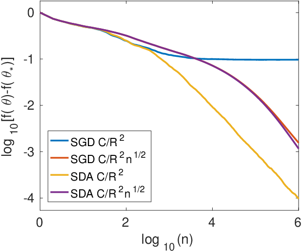
We consider the problem of least-squares regression constrained on the simplex Δd\Delta_{d} of radius r=‖θΣ‖1/2r=\|\theta_{\Sigma}\|_{1}/2 , i.e., minθ∈r​Δd⁡𝔼​(⟨xn,θ⟩−yn)2\min_{\theta\in r\Delta_{d}}\mathbb{E}(\langle x_{n},\theta\rangle-y_{n})^{2}, for d=100d=100. We compare the performance of SDA and SGD algorithms with different settings of the step-size γn\gamma_{n}, constant or proportional to 1/n1/\sqrt{n}. In the left plot of Figure 1 we show the performance on the objective function and on the right plot, we show the performance on the squared Mahalanobis norm ∥⋅∥Σ2\|\cdot\|_{\Sigma}^{2}. All costs are shown in log-scale, normalized so that the first iteration leads to f⁡(θ0)−f⁡(θ∗)=1f(\theta_{0})-f(\theta_{*})=1. We can make the following observations (we only show results on Euclidean geometry since results under the negative entropy geometry were very similar):

  • •

    With constant step-size, SDA converges to the solution at rate O⁡(1/n)O(1/n) whereas the SGD algorithm does not converge to the optimal solution.

  • •

    With decaying step-size γn=1/(2​R2​n)\gamma_{n}=1/(2R^{2}\sqrt{n}), SDA and SGD converge first at rate O⁡(1/n)O(1/\sqrt{n}), then at rate O⁡(1/n)O(1/n), taking finally advantage of the strong-convexity of the problem.

  • •

    We note (a) there is no empirical difference between the performance on the objective function and the squared distance ∥⋅∥Σ2\|\cdot\|_{\Sigma}^{2}, (b) with decreasing step-size, SGD and SDA behave very similarly.
Refer to caption
Refer to caption
Figure 1: Simplex-constrained least-squares regression with synthetic data. Left: Performance on the objective function. Right: Performance on the Mahalanobis norm ∥⋅∥Σ2\|\cdot\|_{\Sigma}^{2}.

6 Conclusion

In this paper, we proposed and analyzed the first algorithm to achieve a convergence rate of O⁡(1/n)O(1/n) for stochastic composite objectives, without the need for strong convexity. This was achieved by considering a constant step-size and averaging of the primal iterates in the dual averaging method.

Our results only apply to expectations of quadratic functions (but to any additional potentially non-smooth terms). In fact, constant step-size stochastic dual averaging is not convergent for general smooth objectives; however, as done in the non-composite case by Bach and Moulines (2013), one could iteratively solved quadratic approximations of the smooth problems with the algorithm we proposed in this paper to achieve the same rate of O⁡(1/n)O(1/n), still with robustness to ill-conditioning and efficient iterations. Finally, it would be worth considering accelerated extensions to achieve a forgetting of initial conditions in O⁡(1/n2)O(1/n^{2}).

Acknowledgements

The authors would like to thank Aymeric Dieuleveut and Damien Garreau for helpful discussions.

References

  • Abernethy et al. [2008] J. Abernethy, E. Hazan, and A. Rakhlin. Competing in the dark: An efficient algorithm for bandit linear optimization. In Proceedings of the International Conference on Learning Theory (COLT), pages 263–274, 2008.
  • Agarwal et al. [2012] A. Agarwal, P. L. Bartlett, P. Ravikumar, and M. J. Wainwright. Information-theoretic lower bounds on the oracle complexity of stochastic convex optimization. IEEE Transactions on Information Theory, 58(5):3235–3249, 2012.
  • Bach [2015] F. Bach. Duality between subgradient and conditional gradient methods. SIAM J. Optim., 25(1):115–129, 2015.
  • Bach and Moulines [2013] F. Bach and E. Moulines. Non-strongly-convex smooth stochastic approximation with convergence rate O⁡(1/n)O(1/n). In Advances in Neural Information Processing Systems (NIPS), December 2013.
  • Bauschke and Borwein [1997] H. H. Bauschke and J. M. Borwein. Legendre functions and the method of random Bregman projections. J. Convex Anal., 4(1):27–67, 1997.
  • Bauschke and Combettes [2011] H. H. Bauschke and P. L. and Combettes. Convex analysis and monotone operator theory in Hilbert spaces. CMS Books in Mathematics/Ouvrages de Mathématiques de la SMC. Springer, New York, 2011.
  • Bauschke et al. [2016] H. H. Bauschke, J. Bolte, and M. Teboulle. A descent lemma beyond lipschitz gradient continuity: first-order methods revisited and applications. Mathematics of Operations Research, 2016.
  • Beck and Teboulle [2003] A. Beck and M. Teboulle. Mirror descent and nonlinear projected subgradient methods for convex optimization. Oper. Res. Lett., 31(3):167–175, 2003.
  • Beck and Teboulle [2009] A. Beck and M. Teboulle. A fast iterative shrinkage-thresholding algorithm for linear inverse problems. SIAM J. Imaging Sci., 2(1):183–202, 2009.
  • Boyd and Vandenberghe [2004] S. Boyd and L. Vandenberghe. Convex optimization. Cambridge University Press, Cambridge, 2004.
  • Bregman [1967] L. M. Bregman. A relaxation method of finding a common point of convex sets and its application to the solution of problems in convex programming. Ž. Vyčisl. Mat. i Mat. Fiz., 7:620–631, 1967.
  • Cesa-Bianchi and Lugosi [2006] N. Cesa-Bianchi and G. Lugosi. Prediction, learning, and games. Cambridge University Press, Cambridge, 2006.
  • Colin et al. [2016] I. Colin, A. Bellet, J. Salmon, and S. Clémençon. Gossip dual averaging for decentralized optimization of pairwise functions. In Proceedings of the conference on machine learning (ICML), 2016.
  • Combettes and Pesquet [2011] P. L. Combettes and J.-C. Pesquet. Proximal splitting methods in signal processing. In Fixed-point algorithms for inverse problems in science and engineering, volume 49 of Springer Optim. Appl., pages 185–212. Springer, New York, 2011.
  • Defazio et al. [2014] A. Defazio, F. Bach, and S. Lacoste-Julien. SAGA: A fast incremental gradient method with support for non-strongly convex composite objectives. In Advances in Neural Information Processing Systems (NIPS), pages 1646–1654, 2014.
  • Dekel et al. [2012] O. Dekel, R. Gilad-Bachrach, O. Shamir, and L. Xiao. Optimal distributed online prediction using mini-batches. J. Mach. Learn. Res., 13:165–202, 2012.
  • Devolder et al. [2013] O. Devolder, F. Glineur, and Y. Nesterov. First-order methods with inexact oracle: the strongly convex case. CORE Discussion Papers, 2013016, 2013.
  • Devroye et al. [1996] L. Devroye, L. Györfi, and G. Lugosi. A probabilistic theory of pattern recognition, volume 31 of Applications of Mathematics (New York). Springer-Verlag, New York, 1996.
  • Dieuleveut et al. [2016] A. Dieuleveut, N. Flammarion, and F. Bach. Harder, better, faster, stronger convergence rates for least-squares regression. arXiv preprint arXiv:1602.05419v2, 2016.
  • Duchi and Ruan [2016] J. Duchi and F. Ruan. Local asymptotics for some stochastic optimization problems: Optimality, constraint identification, and dual averaging. arXiv preprint arXiv:1612.05612, 2016.
  • Duchi et al. [2010] J. Duchi, S. Shalev-Shwartz, Y. Singer, and A. Tewari. Composite objective mirror descent. In Proceedings of the International Conference on Learning Theory (COLT), pages 14–26, 2010.
  • Duchi et al. [2012] J. Duchi, A. Agarwal, and M. Wainwright. Dual averaging for distributed optimization: convergence analysis and network scaling. IEEE Trans. Automat. Control, 57(3):592–606, 2012.
  • Flammarion and Bach [2015] N. Flammarion and F. Bach. From averaging to acceleration, there is only a step-size. In Proceedings of the International Conference on Learning Theory (COLT), 2015.
  • Gentile and Littlestone [1999] C. Gentile and N. Littlestone. The robustness of the pp-norm algorithms. In Proceedings of the International Conference on Learning Theory (COLT), pages 1–11, 1999.
  • Hanner [1956] O. Hanner. On the uniform convexity of LpL^{p} and lpl^{p}. Ark. Mat., 3:239–244, 1956.
  • Hiriart-Urruty and Lemaréchal [2001] J.-B. Hiriart-Urruty and C. Lemaréchal. Fundamentals of convex analysis. Grundlehren Text Editions. Springer-Verlag, Berlin, 2001.
  • Jain et al. [2016] P. Jain, S. M. Kakade, R. Kidambi, P. Netrapalli, and A. Sidford. Parallelizing stochastic approximation through mini-batching and tail-averaging. arXiv preprint arXiv:1610.03774, 2016.
  • Juditsky and Nemirovski [2000] A. Juditsky and A. S. Nemirovski. Functional aggregation for nonparametric regression. Ann. Statist., 28(3):681–712, 2000.
  • Kalai and Vempala [2005] A. Kalai and S. Vempala. Efficient algorithms for online decision problems. J. Comput. System Sci., 71(3):291–307, 2005.
  • Kivinen and Warmuth [1997] J. Kivinen and M. K. Warmuth. Exponentiated gradient versus gradient descent for linear predictors. Inform. and Comput., 132(1):1–63, 1997.
  • Kiwiel [1997] K. C. Kiwiel. Proximal minimization methods with generalized Bregman functions. SIAM J. Control Optim., 35(4):1142–1168, 1997.
  • Krichene et al. [2015] W. Krichene, A. Bayen, and P. L. Bartlett. Accelerated mirror descent in continuous and discrete time. In Advances in Neural Information Processing Systems (NIPS), pages 2845–2853, 2015.
  • Kushner and Yin [2003] H. Kushner and G G. Yin. Stochastic Approximation and Recursive Algorithms and Applications, volume 35. Springer, 2003.
  • Lecué [2006] G. Lecué. Optimal oracle inequality for aggregation of classifiers under low noise condition. In Learning theory, volume 4005 of Lecture Notes in Comput. Sci., pages 364–378. Springer, Berlin, 2006.
  • Lecué [2007] G. Lecué. Optimal rates of aggregation in classification under low noise assumption. Bernoulli, 13(4):1000–1022, 2007.
  • Lee and Wright [2012] S. Lee and S. J. Wright. Manifold identification in dual averaging for regularized stochastic online learning. J. Mach. Learn. Res., 13:1705–1744, 2012.
  • Lu et al. [2016] H. Lu, R. Freund, and Y. Nesterov. Relatively-smooth convex optimization by first-order methods, and applications. arXiv preprint arXiv:1610.05708, 2016.
  • Macchi [1995] O. Macchi. Adaptive processing: The least mean squares approach with applications in transmission. Wiley West Sussex, 1995.
  • Martinet [1970] B. Martinet. Breve communication. régularisation d’inéquations variationnelles par approximations successives. ESAIM: Mathematical Modelling and Numerical Analysis - Modélisation Mathématique et Analyse Numérique, 4:154–158, 1970.
  • McMahan [2011] H. B. McMahan. Follow-the-regularized-leader and mirror descent: Equivalence theorems and l1 regularization. In AISTATS, pages 525–533, 2011.
  • Moreau [1962] J.-J. Moreau. Fonctions convexes duales et points proximaux dans un espace Hilbertien. C. R. Acad. Sci. Paris, 255:2897–2899, 1962.
  • Nemirovski and Yudin [1979] A. S. Nemirovski and D. B. Yudin. Effective methods for the solution of convex programming problems of large dimensions. Èkonom. i Mat. Metody, 15(1):135–152, 1979.
  • Nemirovsky and Yudin [1983] A. S. Nemirovsky and D. B. Yudin. Problem complexity and method efficiency in optimization. A Wiley-Interscience Publication. John Wiley & Sons, Inc., New York, 1983. Translated from the Russian and with a preface by E. R. Dawson, Wiley-Interscience Series in Discrete Mathematics.
  • Nesterov [2004] Y. Nesterov. Introductory Lectures on Convex Optimization, volume 87 of Applied Optimization. Kluwer Academic Publishers, Boston, MA, 2004.
  • Nesterov [2009] Y. Nesterov. Primal-dual subgradient methods for convex problems. Math. Program., 120(1, Ser. B):221–259, 2009.
  • Nesterov [2013] Y. Nesterov. Gradient methods for minimizing composite functions. Math. Program., 140:125–161, 2013.
  • Polyak and Juditsky [1992] B. T. Polyak and A. B. Juditsky. Acceleration of stochastic approximation by averaging. SIAM J. Control Optim., 30(4):838–855, 1992.
  • Raginsky and Rakhlin [2011] M. Raginsky and A. Rakhlin. Information-based complexity, feedback and dynamics in convex programming. IEEE Trans. Inform. Theory, 57(10):7036–7056, 2011.
  • Rish and Grabarnik [2014] I. Rish and G. Grabarnik. Sparse modeling: theory, algorithms, and applications. CRC press, 2014.
  • Rockafellar [1970] R. T. Rockafellar. Convex analysis. Princeton Mathematical Series, No. 28. Princeton University Press, Princeton, N.J., 1970.
  • Shalev-Shwartz and Kakade [2009] S. Shalev-Shwartz and S. m. Kakade. Mind the duality gap: Logarithmic regret algorithms for online optimization. In Advances in Neural Information Processing Systems (NIPS), pages 1457–1464, 2009.
  • Shalev-Shwartz and Singer [2006] S. Shalev-Shwartz and Y. Singer. Online learning meets optimization in the dual. In Learning theory, volume 4005 of Lecture Notes in Comput. Sci., pages 423–437. Springer, Berlin, 2006.
  • Suzuki [2013] T. Suzuki. Dual averaging and proximal gradient descent for online alternating direction multiplier method. In Proceedings of the conference on machine learning (ICML), pages 392–400, 2013.
  • Tsybakov [2003] A. B. Tsybakov. Optimal rates of aggregation. In Proceedings of the Annual Conference on Computational Learning Theory, 2003.
  • Tsybakov [2008] A. B. Tsybakov. Introduction to Nonparametric Estimation. Springer, 2008.
  • Vial [1983] J.-P. Vial. Strong and weak convexity of sets and functions. Math. Oper. Res., 8(2):231–259, 1983.
  • Wibisono et al. [2016] A. Wibisono, A. C. Wilson, and M. I. Jordan. A variational perspective on accelerated methods in optimization. Proceedings of the National Academy of Sciences, 113(47), 2016.
  • Wilson et al. [2016] A. I. Wilson, B. Recht, and M. I. Jordan. A Lyapunov analysis of momentum methods in optimization. arXiv preprint arXiv:1611.02635v3, 2016.
  • Wright et al. [2009] S. J. Wright, R. D. Nowak, and M. A. T. Figueiredo. Sparse reconstruction by separable approximation. IEEE Trans. Signal Process., 57(7):2479–2493, 2009.
  • Xiao [2010] L. Xiao. Dual averaging methods for regularized stochastic learning and online optimization. J. Mach. Learn. Res., 11:2543–2596, 2010.
  • Zinkevich [2003] M. Zinkevich. Online convex programming and generalized infinitesimal gradient ascent. In Proceedings of the conference on machine learning (ICML), 2003.

Appendix A Unambiguity of the primal iterate

We describe here conditions under which the primal iterate θn\theta_{n} in Eq. (3) is correctly defined. Since hh is strictly convex, hn∗h_{n}^{*} is continuously differentiable on dom ̊​hn∗\mathring{\text{dom }}h_{n}^{*} [see Hiriart-Urruty and Lemaréchal, 2001, Theorem 4.1.1]. Therefore the primal iterate θn\theta_{n} is well defined if the dual iterate ηn∈dom ̊​hn∗\eta_{n}\in\mathring{\text{dom }}h_{n}^{*}. It is, for example, the case under two natural assumptions as shown by the next lemma which is an adaption of Lemma 2 by Bauschke et al. [2016].

Lemma 1.

We make the following assumptions:

(B1)

hh or gg is supercoercive.

(B2)

argminθ∈𝒳ψ⁡(θ)\mathop{\rm argmin}_{\theta\in\mathcal{X}}\psi(\theta) is compact and hh bounded below.

Under (B1) or (B2) the primal iterates (θn)(\theta_{n}) defined in Eq. (3) are well defined.

Proof.

Since hh is strictly convex, hn∗h_{n}^{*} is continuously differentiable on dom ̊​hn∗\mathring{\text{dom }}h_{n}^{*} [see Hiriart-Urruty and Lemaréchal, 2001, Theorem 4.1.1]. Therefore the primal iterate θn\theta_{n} is well defined if the dual iterate ηn∈dom ̊​hn∗\eta_{n}\in\mathring{\text{dom }}h_{n}^{*}.

  • •

    If hh or gg is supercoercive then hnh_{n} is supercoercive [see Bauschke and Combettes, 2011, Proposition 11.13] and it follows from Hiriart-Urruty and Lemaréchal [2001, Chapter E, Proposition 1.3.8] that dom ​hn∗=ℝd\text{dom }h_{n}^{*}={\mathbb{R}^{d}}.

  • •

    If argminθ∈𝒳{ψ⁡(θ)}\mathop{\rm argmin}_{\theta\in\mathcal{X}}\{\psi(\theta)\} is compact then ψ+𝟙𝒳\psi+\mathbbm{1}_{\mathcal{X}} is coercive. Moreover

    hn∗​(ηn)\displaystyle h_{n}^{*}(\eta_{n}) =\displaystyle= supθ∈𝒳{⟨ηn,θ⟩−hn​(θ)}​ since​𝒳⊂dom ¯​h\displaystyle\sup_{\theta\in\mathcal{X}}\big\{\langle\eta_{n},\theta\rangle-h_{n}(\theta)\big\}\text{ since}\mathcal{X}\subset\overline{\text{dom }}h
    =\displaystyle= −infθ∈𝒳{h(θ)+γ∑i=1n(g(θ)+f(θi−1)+⟨∇f(θi−1),θ−θi−1⟩)}\displaystyle-\inf_{\theta\in\mathcal{X}}\Big\{h(\theta)+\gamma\sum_{i=1}^{n}(g(\theta)+f(\theta_{i-1})+\langle\nabla f(\theta_{i-1}),\theta-\theta_{i-1}\rangle)\Big\}
    +γ∑i=1n(f(θi−1)−⟨∇f(θi−1),θi−1⟩)\displaystyle+\gamma\sum_{i=1}^{n}(f(\theta_{i-1})-\langle\nabla f(\theta_{i-1}),\theta_{i-1}\rangle)
    ≤\displaystyle\leq −infθ∈𝒳{h(θ)+nγ(g(θ)+f(θ))} by convexity of f\displaystyle-\inf_{\theta\in\mathcal{X}}\big\{h(\theta)+n\gamma(g(\theta)+f(\theta))\big\}\text{ by convexity of }f
    +γ∑i=1n(f(θi−1)−⟨∇f(θi−1),θi−1⟩).\displaystyle+\gamma\sum_{i=1}^{n}(f(\theta_{i-1})-\langle\nabla f(\theta_{i-1}),\theta_{i-1}\rangle).

    Therefore ηn∈dom ̊​hn∗\eta_{n}\in\mathring{\text{dom }}h_{n}^{*} since ψ+𝟙𝒳\psi+\mathbbm{1}_{\mathcal{X}} is coercive and hh bounded below [see Bauschke and Combettes, 2011, Proposition 11.15].

∎

Appendix B Proof of convergence of deterministic DA

We first describe a new notion of smoothness defined by Bauschke et al. [2016]. Then we present our extension of the Bregman divergence to the non-smooth function gg to finally prove Proposition 1.

B.1 A Lipschitz-like/convexity condition

Classical results on the convergence of optimization algorithms in non-Euclidean geometry assume on one hand that the function hh is strongly convex and on the other hand the function ff is Lipschitz or smooth. Following Bauschke et al. [2016], Lu et al. [2016], we consider a different assumption which combines the smoothness of ff and the strong convexity of hh on a single condition called Lipschitz-like/Convexity Condition by Bauschke et al. [2016] and denoted by (LC):

(LC)

There exists a constant L∈ℝL\in\mathbb{R} such that L​h−fLh-f is convex on 𝒳̊\mathring{\mathcal{X}}.

For Euclidean geometry, this condition is obviously equivalent to the smoothness of the function ff with regards to the ℓ2\ell_{2}-norm. Moreover, under an arbitrary norm ∥⋅∥\|\cdot\|, assuming hh μ\mu-strongly convex and ff LL-smooth clearly implies, by simple convex computation, (LC) with constant L/μL/\mu. However (LC) is much more general and may hold even when ff is non-smooth what precisely justifies the introduction of this condition. Many examples are described by Bauschke et al. [2016], Lu et al. [2016]. Furthermore this notion has the elegance of pairing well with Bregman divergences and leading to more refined proofs as shown in the following proposition which summarizes equivalent properties of (LC).

Proposition 4 (Bauschke et al. [2016]).

Assume (A1-4). For L>0L>0 the following conditions are equivalent:

  • •

    L​h−fLh-f is convex on 𝒳̊\mathring{\mathcal{X}}, i.e., (LC) holds,

  • •

    Df​(α,β)≤L​Dh​(α,β)D_{f}(\alpha,\beta)\leq LD_{h}(\alpha,\beta) for all (α,β)∈𝒳×𝒳̊(\alpha,\beta)\in{\mathcal{X}}\times\mathring{\mathcal{X}}.

Furthermore, when ff and hh are assumed twice differentiable, then the above is equivalent to

∇2f​(θ)≼L​∇2h​(θ) for all ​θ∈𝒳̊.\nabla^{2}f(\theta)\preccurlyeq L\nabla^{2}h(\theta)\quad\text{ for all }\theta\in\mathring{\mathcal{X}}.

B.2 Generalized Bregman divergence

The Bregman divergence was defined by Bregman [1967] for a differentiable convex function hh as

Dh(α,β)=h(α)−h(β)−⟨∇h(β),α−β), for (α,β)∈dom h×dom ̊h.D_{h}(\alpha,\beta)=h(\alpha)-h(\beta)-\langle\nabla h(\beta),\alpha-\beta),\text{ for }(\alpha,\beta)\in\text{dom }h\times\mathring{\text{dom }}h. (11)

It behaves as a squared distance depending on the function hh and extends the computational properties of the squared ℓ2\ell_{2}-norm to non-Euclidean spaces. Indeed most proofs in Euclidean space rest upon the expansion ∥θn−θ∗−γ∇f(θn)∥22=∥θn−θ∗∥22+γ2∥∇f(θn)∥22−2γ⟨∇f(θn),θn−θ∗⟩\|\theta_{n}-\theta_{*}-\gamma\nabla f(\theta_{n})\|_{2}^{2}=\|\theta_{n}-\theta_{*}\|_{2}^{2}+\gamma^{2}\|\nabla f(\theta_{n})\|_{2}^{2}-2\gamma\langle\nabla f(\theta_{n}),\theta_{n}-\theta_{*}\rangle which is not available in non-Euclidean geometry. Therefore the Bregman divergence comes to rescue and is used to compute a deviation between the current iterate of the algorithm and the solution of the problem and, seemingly, used as an non-Euclidean Lyapunov function. It has been widely used in optimization [see, e.g., Bauschke and Borwein, 1997, for a review].

We follow this path and include the regularization component gg of the objective function ψ=f+g\psi=f+g in the Bregman divergence for the sake of the analysis. If gg was differentiable we would simply use Dh+n​γ​gD_{h+n\gamma g}. Since gg is not differentiable, DhnD_{h_{n}} is not well defined. However for (α,η)∈dom ​h×dom ̊​hn∗(\alpha,\eta)\in\text{dom }h\times\mathring{\text{dom }}h_{n}^{*}, we denote by extension for θ=∇hn∗​(η)\theta=\nabla h_{n}^{*}(\eta):

D~n​(α,η)=hn​(α)−hn​(θ)−⟨η,α−θ⟩.\tilde{D}_{n}(\alpha,\eta)=h_{n}(\alpha)-h_{n}(\theta)-\langle\eta,\alpha-\theta\rangle. (12)

This extension is different from the one defined by Kiwiel [1997]. It is worth noting that if there exists μ\mu such that α=∇hn∗​(μ)\alpha=\nabla h_{n}^{*}(\mu), we recover the classical formula D~n​(α,η)=Dhn∗​(η,μ)\tilde{D}_{n}(\alpha,\eta)=D_{h_{n}^{*}}(\eta,\mu) which is well defined since hn∗h_{n}^{*} is differentiable. Yet D~n\tilde{D}_{n} is defined more generally since such a μ\mu does not always exist. The next lemma relates D~n\tilde{D}_{n} to DhD_{h} and is obvious if gg is differentiable since Dhn=Dh+γ​n​DgD_{h_{n}}=D_{h}+\gamma nD_{g}.

Lemma 2.

Let n≥0n\geq 0, α∈dom ​h\alpha\in\text{dom }h and η∈dom ̊​hn∗\eta\in\mathring{\text{dom }}h_{n}^{*}, then with θ=∇hn∗​(η)\theta=\nabla h_{n}^{*}(\eta),

D~n​(α,η)≥Dh​(α,θ).\tilde{D}_{n}(\alpha,\eta)\geq D_{h}(\alpha,\theta). (13)
Proof.

θ=∇hn∗​(η)\theta=\nabla h_{n}^{*}(\eta), thus η∈∂hn​(θ)\eta\in\partial h_{n}(\theta) and by elementary calculus rule ∂hn​(θ)=∇h​(θ)+n​γ​∂g⁡(θ)\partial h_{n}(\theta)=\nabla h(\theta)+n\gamma\partial g(\theta). Consequently η−∇h​(θ)∈n​γ​∂g⁡(θ)\eta-\nabla h(\theta)\in n\gamma\partial g(\theta) and by convexity of gg

D~n​(α,η)−Dh​(α,θ)=n​γ​[g⁡(α)−g⁡(θ)−⟨η−∇h​(θ)γ​n,α−θ⟩]≥0.\tilde{D}_{n}(\alpha,\eta)-D_{h}(\alpha,\theta)=n\gamma\bigg[g(\alpha)-g(\theta)-\bigg\langle\frac{\eta-\nabla h(\theta)}{\gamma n},\alpha-\theta\bigg\rangle\bigg]\geq 0.

∎

B.3 Proof of Proposition 1

We assume their exists a constant L>0L>0 such that L​h−fLh-f is convex on 𝒳̊\mathring{\mathcal{X}} and we assume the step-size γ≤1/L\gamma\leq 1/L. We first show that the Bregman divergence decreases along the iterates [Beck and Teboulle, 2003, Bach, 2015, see, e.g.,]. For all θ∈𝒳\theta\in\mathcal{X},

D~n​(θ,ηn)−D~n−1​(θ,ηn−1)\displaystyle\tilde{D}_{n}(\theta,\eta_{n})-\tilde{D}_{n-1}(\theta,\eta_{n-1}) =\displaystyle= hn−1​(θn−1)−hn​(θn)+hn​(θ)−hn−1​(θ)\displaystyle h_{n-1}(\theta_{n-1})-h_{n}(\theta_{n})+h_{n}(\theta)-h_{n-1}(\theta)
−⟨ηn,θ−θn⟩+⟨ηn−1,θ−θn−1⟩\displaystyle-\langle\eta_{n},\theta-\theta_{n}\rangle+\langle\eta_{n-1},\theta-\theta_{n-1}\rangle
=\displaystyle= hn−1​(θn−1)−hn−1​(θn)−γ⁡(g⁡(θn)−g⁡(θ))\displaystyle h_{n-1}(\theta_{n-1})-h_{n-1}(\theta_{n})-\gamma(g(\theta_{n})-g(\theta))
+⟨ηn−1,θn−θn−1⟩+⟨ηn−ηn−1,θn−θ⟩\displaystyle+\langle\eta_{n-1},\theta_{n}-\theta_{n-1}\rangle+\langle\eta_{n}-\eta_{n-1},\theta_{n}-\theta\rangle
=\displaystyle= −D~n−1​(θn,ηn−1)−γ⁡(g⁡(θn)−g⁡(θ))−γ⁡⟨∇f​(θn−1),θn−θ⟩.\displaystyle-\tilde{D}_{n-1}(\theta_{n},\eta_{n-1})-\gamma(g(\theta_{n})-g(\theta))-\gamma\langle\nabla f(\theta_{n-1}),\theta_{n}-\theta\rangle.

Therefore for all θ∈𝒳\theta\in\mathcal{X},

D~n​(θ,ηn)−D~n−1​(θ,ηn−1)=−D~n−1​(θn,ηn−1)+γ⁡⟨∇f​(θn−1),θn−1−θn⟩−γ⁡(g⁡(θn)−g⁡(θ))−γ⁡⟨∇f​(θn−1),θn−1−θ⟩.\tilde{D}_{n}(\theta,\eta_{n})-\tilde{D}_{n-1}(\theta,\eta_{n-1})=-\tilde{D}_{n-1}(\theta_{n},\eta_{n-1})+\gamma\langle\nabla f(\theta_{n-1}),\theta_{n-1}-\theta_{n}\rangle\\ -\gamma(g(\theta_{n})-g(\theta))-\gamma\langle\nabla f(\theta_{n-1}),\theta_{n-1}-\theta\rangle. (14)

It follows from Proposition 4 and Lemma 2

f⁡(θn)−f⁡(θn−1)+⟨∇f​(θn−1),θn−θn−1⟩≤L​Dh​(θn,θn−1)≤L​Dn−1​(θn,θn−1),f(\theta_{n})-f(\theta_{n-1})+\langle\nabla f(\theta_{n-1}),\theta_{n}-\theta_{n-1}\rangle\leq LD_{h}(\theta_{n},\theta_{n-1})\leq LD_{n-1}(\theta_{n},\theta_{n-1}),

and from the convexity of ff,

−⟨∇f​(θn−1),θn−1−θ⟩≤f⁡(θ)−f⁡(θn−1).-\langle\nabla f(\theta_{n-1}),\theta_{n-1}-\theta\rangle\leq f(\theta)-f(\theta_{n-1}).

And Eq. (14) is bounded by

D~n​(θ,ηn)−D~n−1​(θ,ηn−1)≤γ⁡(ψ⁡(θ)−ψ⁡(θn))+(γ​L−1)​Dh​(θn,θn−1).\tilde{D}_{n}(\theta,\eta_{n})-\tilde{D}_{n-1}(\theta,\eta_{n-1})\leq\gamma(\psi(\theta)-\psi(\theta_{n}))+(\gamma L-1)D_{h}(\theta_{n},\theta_{n-1}).

Thus for γ≤1/L\gamma\leq 1/L,

D~n​(θ,ηn)−D~n−1​(θ,ηn−1)≤γ⁡(ψ⁡(θ)−ψ⁡(θn)).\tilde{D}_{n}(\theta,\eta_{n})-\tilde{D}_{n-1}(\theta,\eta_{n-1})\leq\gamma(\psi(\theta)-\psi(\theta_{n})).

Taking θ=θn−1\theta=\theta_{n-1} we note that the sequence {ψ⁡(θn)}n≥0\{\psi(\theta_{n})\}_{n\geq 0} is decreasing and we obtain for γ≤1/L\gamma\leq 1/L,

ψ⁡(θn)−ψ⁡(θ)≤1n+1​∑k=0n[ψ⁡(θi)−ψ⁡(θ)]≤Dh​(θ,θ0)−D~n​(θ,ηn)γ⁡(n+1).\psi(\theta_{n})-\psi(\theta)\leq\frac{1}{n+1}\sum_{k=0}^{n}[\psi(\theta_{i})-\psi(\theta)]\leq\frac{D_{h}(\theta,\theta_{0})-\tilde{D}_{n}(\theta,\eta_{n})}{\gamma(n+1)}. (15)

We assume now that the non-smooth part g=0g=0 and there exists μ≥0\mu\geq 0 such that f−μ​hf-\mu h is convex. So Proposition 4 implies

−⟨∇f​(θn−1),θn−1−θ⟩≤f⁡(θ)−f⁡(θn−1)−μ​Dh​(θ,θn−1),-\langle\nabla f(\theta_{n-1}),\theta_{n-1}-\theta\rangle\leq f(\theta)-f(\theta_{n-1})-\mu D_{h}(\theta,\theta_{n-1}),

which gives with Eq. (14) the better bound

Dh​(θ,θn)−Dh​(θ,θn−1)≤γ⁡(f⁡(θ)−f⁡(θn))−γ​μ​Dh​(θ,θn−1)+(γ​L−1)​Dh​(θn,θn−1).D_{h}(\theta,\theta_{n})-D_{h}(\theta,\theta_{n-1})\leq\gamma(f(\theta)-f(\theta_{n}))-\gamma\mu D_{h}(\theta,\theta_{n-1})+(\gamma L-1)D_{h}(\theta_{n},\theta_{n-1}).

And for γ≤1/L\gamma\leq 1/L, this can be simplified as

Dh​(θ,θn)≤(1−γ​μ)​Dh​(θ,θn−1)+γ⁡(f⁡(θ)−f⁡(θn)).D_{h}(\theta,\theta_{n})\leq(1-\gamma\mu)D_{h}(\theta,\theta_{n-1})+\gamma(f(\theta)-f(\theta_{n})).

The sequence {f⁡(θn)}n≥0\{f(\theta_{n})\}_{n\geq 0} is still decreasing and we obtain by expanding the recursion

Dh​(θ,θn)\displaystyle D_{h}(\theta,\theta_{n}) ≤\displaystyle\leq (1−γ​μ)n​Dh​(θ,θ0)+∑k=1n(1−γ​μ)n−k​γ​(f⁡(θ)−f⁡(θk))\displaystyle(1-\gamma\mu)^{n}D_{h}(\theta,\theta_{0})+\sum_{k=1}^{n}(1-\gamma\mu)^{n-k}\gamma(f(\theta)-f(\theta_{k}))
≤\displaystyle\leq (1−γ​μ)n​Dh​(θ,θ0)+∑k=1n(1−γ​μ)n−k​γ​(f⁡(θ)−f⁡(θk))\displaystyle(1-\gamma\mu)^{n}D_{h}(\theta,\theta_{0})+\sum_{k=1}^{n}(1-\gamma\mu)^{n-k}\gamma(f(\theta)-f(\theta_{k}))
≤\displaystyle\leq (1−γ​μ)n​Dh​(θ,θ0)+∑k=1n(1−γ​μ)n−k​γ​(f⁡(θ)−f⁡(θn))\displaystyle(1-\gamma\mu)^{n}D_{h}(\theta,\theta_{0})+\sum_{k=1}^{n}(1-\gamma\mu)^{n-k}\gamma(f(\theta)-f(\theta_{n}))
≤\displaystyle\leq (1−γ​μ)n​Dh​(θ,θ0)+γ​1−(1−γ​μ)nγ​μ​(f⁡(θ)−f⁡(θn)).\displaystyle(1-\gamma\mu)^{n}D_{h}(\theta,\theta_{0})+\gamma\frac{1-(1-\gamma\mu)^{n}}{\gamma\mu}(f(\theta)-f(\theta_{n})).

Thus for all θ∈𝒳\theta\in\mathcal{X},

1−(1−γ​μ)nμ​(f⁡(θn)−f⁡(θ))+Dh​(θ,θn)≤(1−γ​μ)n​Dh​(θ,θ0),\frac{1-(1-\gamma\mu)^{n}}{\mu}(f(\theta_{n})-f(\theta))+D_{h}(\theta,\theta_{n})\leq(1-\gamma\mu)^{n}D_{h}(\theta,\theta_{0}),

and

f⁡(θn)−f⁡(θ)≤γ​μ​(1−γ​μ)n1−(1−γ​μ)n​Dh​(θ,θ0)γ≤(1−γ​μ)n​Dh​(θ,θ0)γ,f(\theta_{n})-f(\theta)\leq\frac{\gamma\mu(1-\gamma\mu)^{n}}{1-(1-\gamma\mu)^{n}}\frac{D_{h}(\theta,\theta_{0})}{\gamma}\leq(1-\gamma\mu)^{n}\frac{D_{h}(\theta,\theta_{0})}{\gamma},

since (1−γ​μ)2≤1−γ​μ(1-\gamma\mu)^{2}\leq 1-\gamma\mu implies γ​μ/(1−(1−γ​μ)n)≤1\gamma\mu/(1-(1-\gamma\mu)^{n})\leq 1.

Appendix C Proof of Proposition 2

In this section, we will prove Proposition 2. The proof relies on considering the difference between the iteration with noise we denote by (ηn,θn)(\eta_{n},\theta_{n}) and without noise we denote by (ωn,ϕn)(\omega_{n},\phi_{n}), which happens to verify a similar recursion as the SDA recursion.

  • •

    We first show in Lemma 3 that the distance 𝔼​‖ηn−ωn‖Σ−12\mathbb{E}\|\eta_{n}-\omega_{n}\|_{\Sigma^{-1}}^{2} is of order nn.

  • •

    Then in Lemma 4 we show that 𝔼​‖θ¯n−ϕ¯n‖Σ2\mathbb{E}\|\bar{\theta}_{n}-\bar{\phi}_{n}\|_{\Sigma}^{2} is of order O⁡(1/n)O(1/n), by: (a) noticing that 𝔼​‖θ¯n−ϕ¯n‖Σ2\mathbb{E}\|\bar{\theta}_{n}-\bar{\phi}_{n}\|_{\Sigma}^{2} is of order 𝔼​‖ηn−ωn‖Σ−12n2+variancen\frac{\mathbb{E}\|\eta_{n}-\omega_{n}\|_{\Sigma^{-1}}^{2}}{n^{2}}+\frac{\text{variance}}{n}, (b) combining this with the result of Lemma 3.

C.1 Two technical lemmas

We first present and prove two technical lemmas.

C.1.1 Bound on the difference of two dual iterates

In the following lemma we show that the difference between two dual iterates that follow the same recursion is of order nn. This will be used with the iteration with noise (ηn,θn)(\eta_{n},\theta_{n}) and without noise (ωn,ϕn)(\omega_{n},\phi_{n}).

Lemma 3.

Let us consider two sequences of iterates (μk,αk)(\mu_{k},\alpha_{k}) and (νk,βk)(\nu_{k},\beta_{k}) which satisfy the recursion μn−νn=μn−1−νn−1−γ​Σ​(αn−1−βn−1)+γ​ξn\mu_{n}-\nu_{n}=\mu_{n-1}-\nu_{n-1}-\gamma\Sigma(\alpha_{n-1}-\beta_{n-1})+\gamma\xi_{n}, αn=∇hn∗​(μn)\alpha_{n}=\nabla h_{n}^{*}(\mu_{n}) and βn=∇hn∗​(νn)\beta_{n}=\nabla h_{n}^{*}(\nu_{n}) and assume that γ\gamma is such that 2​h−γ​f2h-\gamma f is convex then for all n≥0n\geq 0

𝔼​‖μn−νn‖Σ−12≤‖μ0−ν0‖Σ−12+n​γ2​trΣ−1​C.\mathbb{E}\|\mu_{n}-\nu_{n}\|_{\Sigma^{-1}}^{2}\leq\|\mu_{0}-\nu_{0}\|_{\Sigma^{-1}}^{2}+n\gamma^{2}\mathop{\rm tr}\Sigma^{-1}C.
Proof.

We first expand the square.

‖μn+1−νn+1‖Σ−12\displaystyle\|\mu_{n+1}-\nu_{n+1}\|_{\Sigma^{-1}}^{2} =\displaystyle= ‖μn−νn‖Σ−12+γ2​‖[Σ⁡(αn−βn)−ξn+1]‖Σ−12\displaystyle\|\mu_{n}-\nu_{n}\|_{\Sigma^{-1}}^{2}+\gamma^{2}\|[\Sigma(\alpha_{n}-\beta_{n})-\xi_{n+1}]\|_{\Sigma^{-1}}^{2}
−2​γ​⟨Σ⁡(αn−βn)−ξn+1,Σ−1​(μn−νn)⟩\displaystyle-2\gamma\langle\Sigma(\alpha_{n}-\beta_{n})-\xi_{n+1},\Sigma^{-1}(\mu_{n}-\nu_{n})\rangle
=\displaystyle= ‖μn−νn‖Σ−12+γ2​‖αn−βn‖Σ2+γ2​‖ξn+1‖Σ−12\displaystyle\|\mu_{n}-\nu_{n}\|_{\Sigma^{-1}}^{2}+\gamma^{2}\|\alpha_{n}-\beta_{n}\|_{\Sigma}^{2}+\gamma^{2}\|\xi_{n+1}\|_{\Sigma^{-1}}^{2}
−2​γ2​⟨αn−βn,ξn+1⟩−2​γ​⟨αn−βn−Σ−1​ξn+1,μn−νn⟩.\displaystyle-2\gamma^{2}\langle\alpha_{n}-\beta_{n},\xi_{n+1}\rangle-2\gamma\langle\alpha_{n}-\beta_{n}-\Sigma^{-1}\xi_{n+1},\mu_{n}-\nu_{n}\rangle.

And taking the expectation

𝔼⁡[‖μn+1−νn+1‖Σ−12|ℱn]\displaystyle\mathbb{E}[\|\mu_{n+1}-\nu_{n+1}\|_{\Sigma^{-1}}^{2}|\mathcal{F}_{n}] =\displaystyle= ‖μn−νn‖Σ−12+γ2​𝔼​[‖ξn+1‖Σ−12|ℱn]\displaystyle\|\mu_{n}-\nu_{n}\|_{\Sigma^{-1}}^{2}+\gamma^{2}\mathbb{E}[\|\xi_{n+1}\|_{\Sigma^{-1}}^{2}|\mathcal{F}_{n}]
+γ2​‖αn−βn‖Σ2−2​γ2​𝔼​[⟨αn−βn,ξn+1⟩|ℱn]\displaystyle+\gamma^{2}\|\alpha_{n}-\beta_{n}\|_{\Sigma}^{2}-2\gamma^{2}\mathbb{E}[\langle\alpha_{n}-\beta_{n},\xi_{n+1}\rangle|\mathcal{F}_{n}]
−2γ𝔼[⟨αn−βn)−Σ−1ξn+1,μn−νn⟩|ℱn]\displaystyle-2\gamma\mathbb{E}[\langle\alpha_{n}-\beta_{n})-\Sigma^{-1}\xi_{n+1},\mu_{n}-\nu_{n}\rangle|\mathcal{F}_{n}]
=\displaystyle= ‖μn−νn‖Σ−12+γ2​trΣ−1​𝔼​[ξn+1⊗ξn+1|ℱn]\displaystyle\|\mu_{n}-\nu_{n}\|_{\Sigma^{-1}}^{2}+\gamma^{2}\mathop{\rm tr}\Sigma^{-1}\mathbb{E}[\xi_{n+1}\otimes\xi_{n+1}|\mathcal{F}_{n}]
+γ2​‖αn−βn‖Σ2−2​γ2​⟨αn−βn,𝔼⁡[ξn+1|ℱn]⟩\displaystyle+\gamma^{2}\|\alpha_{n}-\beta_{n}\|_{\Sigma}^{2}-2\gamma^{2}\langle\alpha_{n}-\beta_{n},\mathbb{E}[\xi_{n+1}|\mathcal{F}_{n}]\rangle
−2γ⟨αn−βn)−Σ−1𝔼[ξn+1|ℱn],μn−νn⟩\displaystyle-2\gamma\langle\alpha_{n}-\beta_{n})-\Sigma^{-1}\mathbb{E}[\xi_{n+1}|\mathcal{F}_{n}],\mu_{n}-\nu_{n}\rangle
=\displaystyle= ‖μn−νn‖Σ−12+γ2​trΣ−1​C\displaystyle\|\mu_{n}-\nu_{n}\|_{\Sigma^{-1}}^{2}+\gamma^{2}\mathop{\rm tr}\Sigma^{-1}C
+γ2​‖αn−βn‖Σ2−2​γ​⟨αn−βn,μn−νn⟩.\displaystyle+\gamma^{2}\|\alpha_{n}-\beta_{n}\|_{\Sigma}^{2}-2\gamma\langle\alpha_{n}-\beta_{n},\mu_{n}-\nu_{n}\rangle.

Moreover, using the definition of αn\alpha_{n} and βn\beta_{n},

γ​‖αn−βn‖Σ2−2​⟨αn−βn,μn−νn⟩\displaystyle\gamma\|\alpha_{n}-\beta_{n}\|_{\Sigma}^{2}-2\langle\alpha_{n}-\beta_{n},\mu_{n}-\nu_{n}\rangle =\displaystyle= ⟨γ​Σ​(αn−βn)−2​(μn−νn),αn−βn⟩\displaystyle\langle\gamma\Sigma(\alpha_{n}-\beta_{n})-2(\mu_{n}-\nu_{n}),\alpha_{n}-\beta_{n}\rangle
=\displaystyle= ⟨γ∇f(αn)−∇f(βn)−2(∇h(αn)−∇h(βn)),αn−βn⟩\displaystyle\langle\gamma\nabla f(\alpha_{n})-\nabla f(\beta_{n})-2(\nabla h(\alpha_{n})-\nabla h(\beta_{n})),\alpha_{n}-\beta_{n}\rangle
−2​⟨(μn−∇h​(αn))−(νn−∇h​(βn)),αn−βn⟩\displaystyle-2\langle(\mu_{n}-\nabla h(\alpha_{n}))-(\nu_{n}-\nabla h(\beta_{n})),\alpha_{n}-\beta_{n}\rangle
=\displaystyle= ⟨∇(γ​f−2​h)​(αn)−∇(γ​f−2​h)​(βn),αn−βn⟩\displaystyle\langle\nabla(\gamma f-2h)(\alpha_{n})-\nabla(\gamma f-2h)(\beta_{n}),\alpha_{n}-\beta_{n}\rangle
−2​⟨(μn−∇h​(αn))−(νn−∇h​(βn)),αn−βn⟩.\displaystyle-2\langle(\mu_{n}-\nabla h(\alpha_{n}))-(\nu_{n}-\nabla h(\beta_{n})),\alpha_{n}-\beta_{n}\rangle.

Using the hh-smoothness of ff and assuming that γ\gamma is such 2​h−γ​f2h-\gamma f is convex,

⟨∇(γ​f−2​h)​(αn)−∇(γ​f−2​h)​(βn),αn−βn⟩≤0,\langle\nabla(\gamma f-2h)(\alpha_{n})-\nabla(\gamma f-2h)(\beta_{n}),\alpha_{n}-\beta_{n}\rangle\leq 0,

and as explained in the proof of Lemma 2, μn−∇h​(αn)∈∂n​γ​g​(αn)\mu_{n}-\nabla h(\alpha_{n})\in\partial n\gamma g(\alpha_{n}) and νn−∇h​(βn)∈∂n​γ​g​(βn)\nu_{n}-\nabla h(\beta_{n})\in\partial n\gamma g(\beta_{n}) and consequently

⟨(μn−∇h​(αn))−(νn−∇h​(βn)),αn−βn⟩≤0,\langle(\mu_{n}-\nabla h(\alpha_{n}))-(\nu_{n}-\nabla h(\beta_{n})),\alpha_{n}-\beta_{n}\rangle\leq 0,

by convexity of gg. This explains that

γ​‖αn−βn‖Σ2−2​⟨αn−βn,μn−νn⟩≤0.\gamma\|\alpha_{n}-\beta_{n}\|_{\Sigma}^{2}-2\langle\alpha_{n}-\beta_{n},\mu_{n}-\nu_{n}\rangle\leq 0.

Then, taking the global expectation, we have shown that

𝔼​‖μn+1−νn+1‖Σ−12≤𝔼​‖μn−νn‖Σ−12+γ2​trΣ−1​C,\mathbb{E}\|\mu_{n+1}-\nu_{n+1}\|_{\Sigma^{-1}}^{2}\leq\mathbb{E}\|\mu_{n}-\nu_{n}\|_{\Sigma^{-1}}^{2}+\gamma^{2}\mathop{\rm tr}\Sigma^{-1}C,

which concludes the proof. ∎

C.1.2 Bound on the difference of the average of two primal iterates

In the following lemma we adapt the classic proof of averaged SGD by Polyak and Juditsky [1992] to show that the difference between two averaged primal iterates, which follow the same recursion, is of order O⁡(1/n)O(1/n).

Lemma 4.

Let us consider two sequences of iterates (μk,αk)(\mu_{k},\alpha_{k}) and (νk,βk)(\nu_{k},\beta_{k}) which satisfy the recursion μn−νn=μn−1−νn−1−γ​Σ​(αn−1−βn−1)+γ​ξn\mu_{n}-\nu_{n}=\mu_{n-1}-\nu_{n-1}-\gamma\Sigma(\alpha_{n-1}-\beta_{n-1})+\gamma\xi_{n}, αn=∇hn∗​(μn)\alpha_{n}=\nabla h_{n}^{*}(\mu_{n}) and βn=∇hn∗​(νn)\beta_{n}=\nabla h_{n}^{*}(\nu_{n}) and assume that γ\gamma is such that 2​h−γ​f2h-\gamma f is convex then for all n≥0n\geq 0

𝔼​‖α¯n−β¯n‖Σ2≤4​‖μ0−ν0‖Σ−12(γ​n)2+4n​trΣ−1​C.{\mathbb{E}\|\bar{\alpha}_{n}-\bar{\beta}_{n}\|_{\Sigma}^{2}}\leq 4\frac{\|\mu_{0}-\nu_{0}\|^{2}_{\Sigma^{-1}}}{(\gamma n)^{2}}+{\frac{4}{n}\mathop{\rm tr}\Sigma^{-1}C}.
Proof.

Let us consider two sequences of iterates (μk,αk)(\mu_{k},\alpha_{k}) and (νk,βk)(\nu_{k},\beta_{k}) which satisfy the recursion μn−νn=μn−1−νn−1−γ​Σ​(αn−1−βn−1)+γ​ξn\mu_{n}-\nu_{n}=\mu_{n-1}-\nu_{n-1}-\gamma\Sigma(\alpha_{n-1}-\beta_{n-1})+\gamma\xi_{n}, αn=∇hn∗​(μn)\alpha_{n}=\nabla h_{n}^{*}(\mu_{n}) and βn=∇hn∗​(νn)\beta_{n}=\nabla h_{n}^{*}(\nu_{n}). This can be written as

Σ⁡(αn−βn)=μn−νn−μn+1+νn+1γ+ξn+1.\Sigma(\alpha_{n}-\beta_{n})=\frac{\mu_{n}-\nu_{n}-\mu_{n+1}+\nu_{n+1}}{\gamma}+\xi_{n+1}.

Thus we obtain

Σ1/2​∑i=0n−1(αi−βi)\displaystyle\Sigma^{1/2}\sum_{i=0}^{n-1}(\alpha_{i}-\beta_{i}) =\displaystyle= Σ−1/2(μ0−ν0−μn+νn)γ+∑i=0n−1Σ−1/2ξi+1.\displaystyle\frac{\Sigma^{-1/2}(\mu_{0}-\nu_{0}-\mu_{n}+\nu_{n})}{\gamma}+\sum_{i=0}^{n-1}\Sigma^{-1/2}\xi_{i+1}.

Finally, using that by convexity (a+b)2≤2​(a2+b2)(a+b)^{2}\leq 2(a^{2}+b^{2}), this leads to

𝔼∥α¯n−β¯n∥Σ2≤2𝔼∥Σ−1/2(μ0−ν0)γ+∑i=0n−1Σ−1/2ξi+1∥22+2𝔼∥Σ−1/2(μn−νn)γ∥22.{\mathbb{E}\|\bar{\alpha}_{n}-\bar{\beta}_{n}\|_{\Sigma}^{2}}\leq 2\mathbb{E}\Big\|\frac{\Sigma^{-1/2}(\mu_{0}-\nu_{0})}{\gamma}+\sum_{i=0}^{n-1}\Sigma^{-1/2}\xi_{i+1}\Big\|_{2}^{2}+2\mathbb{E}\Big\|\frac{\Sigma^{-1/2}(\mu_{n}-\nu_{n})}{\gamma}\Big\|_{2}^{2}.

Using martingale second moment expansions, we obtain

𝔼​‖α¯n−β¯n‖Σ2≤2​𝔼​‖μ0−ν0‖Σ−12(γ​n)2+2​𝔼​‖μn−νn‖Σ−12(γ​n)2+2n2​∑i=0n−1trΣ−1​𝔼​(ξi+1⊗ξi+1).{\mathbb{E}\|\bar{\alpha}_{n}-\bar{\beta}_{n}\|_{\Sigma}^{2}}\leq 2\mathbb{E}\frac{\|\mu_{0}-\nu_{0}\|^{2}_{\Sigma^{-1}}}{(\gamma n)^{2}}+2\frac{{\mathbb{E}\|\mu_{n}-\nu_{n}\|^{2}_{\Sigma^{-1}}}}{(\gamma n)^{2}}+\frac{2}{n^{2}}{\sum_{i=0}^{n-1}\mathop{\rm tr}\Sigma^{-1}\mathbb{E}(\xi_{i+1}\otimes\xi_{i+1})}.

We compute ∑i=0n−1trΣ−1​𝔼​(ξi+1⊗ξi+1)=∑i=0n−1trΣ−1​C=n​trΣ−1​C\sum_{i=0}^{n-1}\mathop{\rm tr}\Sigma^{-1}\mathbb{E}(\xi_{i+1}\otimes\xi_{i+1})=\sum_{i=0}^{n-1}\mathop{\rm tr}\Sigma^{-1}C=n\mathop{\rm tr}\Sigma^{-1}C and, using Lemma 3, we bound 𝔼​‖μn−νn‖Σ−12\mathbb{E}\|\mu_{n}-\nu_{n}\|^{2}_{\Sigma^{-1}} as

𝔼​‖μn−νn‖Σ−12(γ​n)2≤‖μ0−ν0‖Σ−12(γ​n)2+1n​trΣ−1​C.\frac{{\mathbb{E}\|\mu_{n}-\nu_{n}\|^{2}_{\Sigma^{-1}}}}{(\gamma n)^{2}}\leq\frac{\|\mu_{0}-\nu_{0}\|^{2}_{\Sigma^{-1}}}{(\gamma n)^{2}}+{\frac{1}{n}\mathop{\rm tr}\Sigma^{-1}C}.

This implies the final bound

𝔼​‖α¯n−β¯n‖Σ2≤4​‖μ0−ν0‖Σ−12(γ​n)2+4n​trΣ−1​C.{\mathbb{E}\|\bar{\alpha}_{n}-\bar{\beta}_{n}\|_{\Sigma}^{2}}\leq 4\frac{\|\mu_{0}-\nu_{0}\|^{2}_{\Sigma^{-1}}}{(\gamma n)^{2}}+{\frac{4}{n}\mathop{\rm tr}\Sigma^{-1}C}.

∎

C.2 Application of Lemma 4 to prove Proposition 2

First of all we define the sequence

ηn∗=∇h(θ∗)−nγ∇f(θ∗).\eta_{n}^{*}=\nabla h(\theta_{*})-n\gamma\nabla f(\theta_{*}). (16)

By definition of θ∗\theta_{*}, −∇f​(θ∗)∈∂g⁡(θ∗)-\nabla f(\theta_{*})\in\partial g(\theta_{*}) then ηn∗∈∂(h+n​γ​g)​θ∗\eta_{n}^{*}\in\partial(h+n\gamma g)\theta_{*} and θ∗=∇hn∗​(ηn∗)\theta_{*}=\nabla h_{n}^{*}(\eta_{n}^{*}). Therefore the sequence ηn∗\eta_{n}^{*} is obtained by iterating DA started from the solution of the problem θ∗\theta_{*}.

We note then than Lemma 4 applied to (μn=ηn,αn=θn)(\mu_{n}=\eta_{n},\alpha_{n}=\theta_{n}) and (νn=ηn∗,βn=θ∗)(\nu_{n}=\eta_{n}^{*},\beta_{n}=\theta_{*}) gives the first bound of Proposition 2.

On the other hand, when considering the noiseless iterates (ωn,ϕn)(\omega_{n},\phi_{n}) defined by ωn=ωn−1−γ​Σ​(ϕn−1−θΣ)\omega_{n}=\omega_{n-1}-\gamma\Sigma(\phi_{n-1}-\theta_{\Sigma}) and ϕn=∇hn∗​(ωn)\phi_{n}=\nabla h_{n}^{*}(\omega_{n}), started from the same point ϕ0=θ0\phi_{0}=\theta_{0}, we obtain, following Proposition 1, for gamma such that h−γ​fh-\gamma f is convex, the bound

12​‖ϕ¯n−θ∗‖Σ2≤ψ⁡(ϕ¯n)−ψ⁡(θ∗)≤Dh​(θ∗,θ0)γ​n.\frac{1}{2}\|\bar{\phi}_{n}-\theta_{*}\|_{\Sigma}^{2}\leq\psi(\bar{\phi}_{n})-\psi(\theta_{*})\leq\frac{D_{h}(\theta_{*},\theta_{0})}{\gamma n}.

Therefore, considering the difference between the semi-stochastic and the noiseless iterate (ηn−ωn)(\eta_{n}-\omega_{n}) which verifies the same equation ηn−ωn=ηn−1−ωn−1−γ​Σ​(θn−1−ϕn−1)+γ​ξn\eta_{n}-\omega_{n}=\eta_{n-1}-\omega_{n-1}-\gamma\Sigma(\theta_{n-1}-\phi_{n-1})+\gamma\xi_{n} with θ0−ϕ0=0\theta_{0}-\phi_{0}=0 as initial value, we may apply Lemma 4 to show

𝔼​‖θ¯n−ϕ¯n‖Σ2≤4n​trΣ−1​C.{\mathbb{E}\|\bar{\theta}_{n}-\bar{\phi}_{n}\|_{\Sigma}^{2}}\leq{\frac{4}{n}\mathop{\rm tr}\Sigma^{-1}C}.

And by the Cauchy-Schwarz inequality

𝔼​‖θ¯n−θ∗‖Σ2\displaystyle{\mathbb{E}\|\bar{\theta}_{n}-\theta_{*}\|_{\Sigma}^{2}} ≤\displaystyle\leq 2​𝔼​‖θ¯n−ϕ¯n‖Σ2+2​𝔼​‖ϕ¯n−θ∗‖Σ2\displaystyle 2{\mathbb{E}\|\bar{\theta}_{n}-\bar{\phi}_{n}\|_{\Sigma}^{2}}+2{\mathbb{E}\|\bar{\phi}_{n}-\theta_{*}\|_{\Sigma}^{2}}
≤\displaystyle\leq 8n​trΣ−1​C+4​Dh​(θ∗,θ0)γ​n,\displaystyle{\frac{8}{n}\mathop{\rm tr}\Sigma^{-1}C}+4{\frac{D_{h}(\theta_{*},\theta_{0})}{\gamma n}},

which proves the second bound of Proposition 2.

It is worth noting that the condition on the step-size of Lemma 3 is less restrictive than in Proposition 2. Indeed for all γ\gamma such that 2​h−γ​f2h-\gamma f is convex, the difference between the dual iterates of the stochastic and deterministic recursions stay close but the deterministic iterates only converge to the solution for γ\gamma such that h−γ​fh-\gamma f is convex.

Appendix D Proof of Proposition 3

In this section, we prove Proposition 3. The proof technique is similar to Proposition 2 but with the additional difficulty of the multiplicative noise.

We first note that Assumption (A11) is equivalent by the Cauchy-Schwarz inequality to

𝔼⁡⟨xn,M​xn⟩​⟨xn,N​xn⟩≤κ​tr(M​Σ)​tr(N​Σ),\mathbb{E}\langle x_{n},Mx_{n}\rangle\langle x_{n},Nx_{n}\rangle\leq\kappa\mathop{\rm tr}(M\Sigma)\mathop{\rm tr}(N\Sigma), (17)

for all positive semi-definite symmetric matrices MM and NN [Dieuleveut et al., 2016, see, e.,g., proof in]. We will often use, in the following demonstrations, Eq. (17) and its direct corollary

⟨xn,M​xn⟩​xn⊗xn≼κ​tr(M​Σ)​Σ,\langle x_{n},Mx_{n}\rangle x_{n}\otimes x_{n}\preccurlyeq\kappa\mathop{\rm tr}(M\Sigma)\Sigma, (18)

without always referring to it.

D.1 A simple proof for the bounded constrained case

We first prove Proposition 3 for the constrained case. It is then a simple corollary of Proposition 2.

Let us denote by 𝒞\mathcal{C} a bounded convex set and consider the constrained problem (g=𝟏𝒞g=\mathbf{1}_{\mathcal{C}}). We remind that the general stochastic oracle for SDA in least-squares regression is

∇fn​(θ)=(Σ+ζn)​(θ−θΣ)−ξn, for ​θ∈ℝd,\nabla f_{n}(\theta)=(\Sigma+\zeta_{n})(\theta-\theta_{\Sigma})-\xi_{n},\text{ for }\theta\in{\mathbb{R}^{d}},

with ζn=xn⊗xn−Σ\zeta_{n}=x_{n}\otimes x_{n}-\Sigma. We denote by r=maxθ∈𝒞⁡‖θ−θΣ‖2r=\max_{\theta\in\mathcal{C}}\|\theta-\theta_{\Sigma}\|_{2} and we show that the noise covariance is directly bounded, despite the multiplicative noise:

𝔼⁡[(∇fn​(θ)−∇f​(θ))⊗(∇fn​(θ)−∇f​(θ))]≼2​𝔼​[ζn​(θ−θΣ)⊗(θ−θΣ)​ζn]+2​𝔼​ξn⊗ξn,\mathbb{E}\Big[\big(\nabla f_{n}(\theta)-\nabla f(\theta)\big)\otimes\big(\nabla f_{n}(\theta)-\nabla f(\theta)\big)\Big]\preccurlyeq 2\mathbb{E}\big[\zeta_{n}(\theta-\theta_{\Sigma})\otimes(\theta-\theta_{\Sigma})\zeta_{n}\big]+2\mathbb{E}\xi_{n}\otimes\xi_{n},

and using Assumption (A11)

𝔼⁡[ζn​(θ−θΣ)⊗(θ−θΣ)​ζn]≼r2​𝔼​ζn​ζn≼r2​κ​(trΣ)​Σ.\mathbb{E}\big[\zeta_{n}(\theta-\theta_{\Sigma})\otimes(\theta-\theta_{\Sigma})\zeta_{n}\big]\preccurlyeq r^{2}\mathbb{E}\zeta_{n}\zeta_{n}\preccurlyeq r^{2}\kappa(\mathop{\rm tr}\Sigma)\Sigma.

Therefore

𝔼⁡[(∇fn​(θ)−∇f​(θ))⊗(∇fn​(θ)−∇f​(θ))]≼2​(σ2+r2​κ​(trΣ))​Σ.\mathbb{E}\Big[\big(\nabla f_{n}(\theta)-\nabla f(\theta)\big)\otimes\big(\nabla f_{n}(\theta)-\nabla f(\theta)\big)\Big]\preccurlyeq 2\big(\sigma^{2}+r^{2}\kappa(\mathop{\rm tr}\Sigma)\big)\Sigma.

Hence Proposition 2 already implies for all step-size such that h−γ​fh-\gamma f is convex

12​𝔼​‖θ¯n−θ∗‖Σ2≤2​Dh​(θ∗,θ0)γ​n+8​dn​(σ2+κ​r2​trΣ).\frac{1}{2}{\mathbb{E}\|\bar{\theta}_{n}-\theta_{*}\|_{\Sigma}^{2}}\leq 2\frac{D_{h}(\theta_{*},\theta_{0})}{\gamma n}+\frac{8d}{n}(\sigma^{2}+\kappa r^{2}\mathop{\rm tr}\Sigma).

D.2 A general result

We prove in this section a more general result than Proposition 3 under the additional assumption

(A14)

There exists b∈[0,1]b\in[0,1] and μb>0\mu_{b}>0 such that h−μb2∥⋅∥Σb2h-\frac{\mu_{b}}{2}\|\cdot\|_{\Sigma^{b}}^{2} is convex.

Proposition 5.

Assume (A2-4) and (A7-14). Consider the recursion in Eq. (8). For any constant step-size γ\gamma such that γ≤min⁡{μb4​κ​trΣ1−b,1κ​L​d}\gamma\leq\min\{\frac{\mu_{b}}{4\kappa\mathop{\rm tr}\Sigma^{1-b}},\frac{1}{\kappa Ld}\}. Then

12​𝔼​‖θ¯n−θ∗‖Σ2≤2​Dh​(θ∗,θ0)γ​n+24n​trΣ−1​C+16​κ​d​γn​μb​trC​Σ−b+8​κ​dn​(4​κ​γ​trΣ1−bμb+3)​‖θ∗−θΣ‖Σ2+80​κ​dγ​n2​Dh​(θ∗,θ0)+16​κ​dn2​g​(θ0).\frac{1}{2}{\mathbb{E}\|\bar{\theta}_{n}-\theta_{*}\|_{\Sigma}^{2}}\leq{2\frac{D_{h}(\theta_{*},\theta_{0})}{\gamma n}}+\frac{24}{n}\mathop{\rm tr}\Sigma^{-1}C+\frac{16\kappa d\gamma}{n\mu_{b}}\mathop{\rm tr}C\Sigma^{-b}\\ +\frac{8\kappa d}{n}\bigg(\frac{4\kappa\gamma\mathop{\rm tr}\Sigma^{1-b}}{\mu_{b}}+3\bigg)\|\theta_{*}-\theta_{\Sigma}\|_{\Sigma}^{2}+{80\frac{\kappa d}{\gamma n^{2}}}{D_{h}(\theta_{*},\theta_{0})}+\frac{16\kappa d}{n^{2}}g(\theta_{0}).

We note Assumption (14) is always satisfied for b=1b=1, for which it is Assumption (13). Therefore Proposition 5 directly implies Proposition 3 as a corollary. We prove now two auxiliary lemmas which will be used in the proof of the Proposition 5.

D.3 Two auxiliary results for least-squares objectives

For b∈[0,1]b\in[0,1], we denote by TbT_{b} the operator Tb=𝔼⁡[⟨x,Σ−b​x⟩​x⊗x]T_{b}=\mathbb{E}[\langle x,\Sigma^{-b}x\rangle x\otimes x]. We first prove that, for least-square objectives, the sum of the function evaluated along the primal iterates remains bounded.

Lemma 5.

Let us consider the recursion ηn=ηn−1−γ​xn⊗xn​(θn−1−θ∗)+γ​ξn\eta_{n}=\eta_{n-1}-\gamma x_{n}\otimes x_{n}(\theta_{n-1}-\theta_{*})+\gamma\xi_{n} and assume gg is positive and there exist μb\mu_{b} such that h−μb2∥⋅∥Σb2h-\frac{\mu_{b}}{2}\|\cdot\|_{\Sigma^{b}}^{2} is convex and κ\kappa such that Tb≼κ​tr(Σ1−b)​ΣT_{b}\preccurlyeq\kappa\mathop{\rm tr}(\Sigma^{1-b})\Sigma, then for γ≤μb/(4​κ​trΣ1−b)\gamma\leq\mu_{b}/(4\kappa\mathop{\rm tr}\Sigma^{1-b}) and θ∈𝒳\theta\in\mathcal{X} we have

𝔼​∑i=0n[ψ⁡(θi)−ψ⁡(θ)]+(1−4​γ​κ​tr(Σ1−b)/μb)​∑i=0n12​𝔼​‖θi−θ‖Σ2≤Dh​(θ,θ0)−𝔼​Dh​(θ,θn+1)γ+(n+1)γ/μbtrΣ−bC+4(n+1)κtr(Σ1−b)/μbf(θ)+g(θ0).\mathbb{E}\sum_{i=0}^{n}[\psi(\theta_{i})-\psi(\theta)]+\Big(1-4\gamma\kappa\mathop{\rm tr}(\Sigma^{1-b})/\mu_{b}\Big)\sum_{i=0}^{n}\frac{1}{2}\mathbb{E}\|\theta_{i}-\theta\|_{\Sigma}^{2}\\ \leq\frac{D_{h}(\theta,\theta_{0})-\mathbb{E}D_{h}(\theta,\theta_{n+1})}{\gamma}+(n+1)\gamma/\mu_{b}\mathop{\rm tr}\Sigma^{-b}C+4(n+1)\kappa\mathop{\rm tr}(\Sigma^{1-b})/\mu_{b}f(\theta)+g(\theta_{0}).

We note that we can also obtain a bound depending on 2​ψ​(θ)2\psi(\theta) rather than 4​f​(θ)4f(\theta) with a similar proof.

Proof.

Let denote by fn​(θ)=xn⊗xn​(θ−θΣ)+ξnf_{n}(\theta)=x_{n}\otimes x_{n}(\theta-\theta_{\Sigma})+\xi_{n}. Then following the proof of Proposition 1 (see Eq. (14)) we have the expansion

D~n​(θ,ηn)−D~n−1​(θ,ηn−1)≤−γ⁡(g⁡(θn)−g⁡(θ))−γ⁡⟨∇fn​(θn−1),θn−1−θ⟩−Dh​(θn,θn−1)+γ⁡⟨∇fn​(θn−1),θn−1−θn⟩.\tilde{D}_{n}(\theta,\eta_{n})-\tilde{D}_{n-1}(\theta,\eta_{n-1})\leq-\gamma(g(\theta_{n})-g(\theta))-\gamma\langle\nabla f_{n}(\theta_{n-1}),\theta_{n-1}-\theta\rangle\\ -D_{h}(\theta_{n},\theta_{n-1})+\gamma\langle\nabla f_{n}(\theta_{n-1}),\theta_{n-1}-\theta_{n}\rangle. (19)

Since h−μb2∥⋅∥Σb2h-\frac{\mu_{b}}{2}\|\cdot\|_{\Sigma^{b}}^{2} is convex, using Proposition 4, we get that Dh​(θn,θn−1)≥μb2​‖θn−θn−1‖Σb2D_{h}(\theta_{n},\theta_{n-1})\geq\frac{\mu_{b}}{2}\|\theta_{n}-\theta_{n-1}\|_{\Sigma^{b}}^{2}. Let denote by A=−Dh​(θn,θn−1),+γ⁡⟨∇fn​(θn−1),θn−1−θn⟩A=-D_{h}(\theta_{n},\theta_{n-1}),+\gamma\langle\nabla f_{n}(\theta_{n-1}),\theta_{n-1}-\theta_{n}\rangle,

A\displaystyle A ≤\displaystyle\leq −μb2​‖θn−θn−1‖Σb2+γ⁡⟨xn⊗xn​(θn−1−θΣ)+ξn,θn−1−θn⟩\displaystyle-\frac{\mu_{b}}{2}\|\theta_{n}-\theta_{n-1}\|_{\Sigma^{b}}^{2}+\gamma\langle x_{n}\otimes x_{n}(\theta_{n-1}-\theta_{\Sigma})+\xi_{n},\theta_{n-1}-\theta_{n}\rangle
≤\displaystyle\leq −μb2​‖θn−θn−1‖Σb2\displaystyle-\frac{\mu_{b}}{2}\|\theta_{n}-\theta_{n-1}\|_{\Sigma^{b}}^{2}
+⟨γΣ−b/2μb​[xn⊗xn​(θn−1−θΣ)+ξn],Σb/2​μb​θn−1−θn⟩\displaystyle+\Big\langle\frac{\gamma\Sigma^{-b/2}}{\sqrt{\mu_{b}}}[x_{n}\otimes x_{n}(\theta_{n-1}-\theta_{\Sigma})+\xi_{n}],{\Sigma^{b/2}}{\sqrt{\mu_{b}}}\theta_{n-1}-\theta_{n}\Big\rangle
≤\displaystyle\leq γ2​μb2​‖xn⊗xn​(θn−1−θΣ)+ξn‖Σ−b2\displaystyle\frac{\gamma^{2}\mu_{b}}{2}\|x_{n}\otimes x_{n}(\theta_{n-1}-\theta_{\Sigma})+\xi_{n}\|_{\Sigma^{-b}}^{2}
−12​‖γ​Σb/2​μb​(θn−θn−1)−γΣ−b/2μb​[xn⊗xn​(θn−1−θΣ)+ξn]‖22\displaystyle\textstyle-\frac{1}{2}\|{\gamma\Sigma^{b/2}}{\sqrt{\mu_{b}}}(\theta_{n}-\theta_{n-1})-\frac{\gamma\Sigma^{-b/2}}{\sqrt{\mu_{b}}}[x_{n}\otimes x_{n}(\theta_{n-1}-\theta_{\Sigma})+\xi_{n}]\|_{2}^{2}
≤\displaystyle\leq γ22​μb​‖xn⊗xn​(θn−1−θΣ)+ξn‖Σ−12\displaystyle\frac{\gamma^{2}}{2\mu_{b}}\|x_{n}\otimes x_{n}(\theta_{n-1}-\theta_{\Sigma})+\xi_{n}\|_{\Sigma^{-1}}^{2}
≤\displaystyle\leq γ2μb​‖θn−1−θΣ‖Tb2+γ2μb​‖ξn‖Σ−b2.\displaystyle\frac{\gamma^{2}}{\mu_{b}}\|\theta_{n-1}-\theta_{\Sigma}\|_{T_{b}}^{2}+\frac{\gamma^{2}}{\mu_{b}}\|\xi_{n}\|_{\Sigma^{-b}}^{2}.

Thus, taking the conditional expectation and assuming that κ\kappa is such that Tb≼κ​tr(Σ1−b)​ΣT_{b}\preccurlyeq\kappa\mathop{\rm tr}(\Sigma^{1-b})\Sigma we obtain

−𝔼[Dh(θn,θn−1)ℱn−1]+γ𝔼⟨∇fn(θn−1),θn−1−θn⟩ℱn−1]≤γ2​κ​tr(Σ1−b)μb​‖θn−1−θΣ‖Σ2+γ2μb​trΣ−b​C.-\mathbb{E}[D_{h}(\theta_{n},\theta_{n-1})\mathcal{F}_{n-1}]+\gamma\mathbb{E}\langle\nabla f_{n}(\theta_{n-1}),\theta_{n-1}-\theta_{n}\rangle\mathcal{F}_{n-1}]\\ \leq\frac{\gamma^{2}\kappa\mathop{\rm tr}(\Sigma^{1-b})}{\mu_{b}}\|\theta_{n-1}-\theta_{\Sigma}\|_{\Sigma}^{2}+\frac{\gamma^{2}}{\mu_{b}}\mathop{\rm tr}\Sigma^{-b}C.

Taking again the conditional expectation in Eq. (19), we have for θ∈𝒳\theta\in\mathcal{X}

𝔼⁡[D~n​(θ,ηn)|ℱn−1]−D~n−1​(θ,ηn−1)\displaystyle\mathbb{E}[\tilde{D}_{n}(\theta,\eta_{n})|\mathcal{F}_{n-1}]-\tilde{D}_{n-1}(\theta,\eta_{n-1}) ≤\displaystyle\leq γ2​κμb​tr(Σ1−b)​‖θn−1−θΣ‖Σ2+γ2μb​trΣ−b​C\displaystyle\frac{\gamma^{2}\kappa}{\mu_{b}}\mathop{\rm tr}(\Sigma^{1-b})\|\theta_{n-1}-\theta_{\Sigma}\|_{\Sigma}^{2}+\frac{\gamma^{2}}{{\mu_{b}}}\mathop{\rm tr}\Sigma^{-b}C
−γ​𝔼​[⟨xn⊗xn​(θn−1−θΣ)+ξn,θn−1−θ⟩|ℱn−1]\displaystyle-\gamma\mathbb{E}[\langle x_{n}\otimes x_{n}(\theta_{n-1}-\theta_{\Sigma})+\xi_{n},\theta_{n-1}-\theta\rangle|\mathcal{F}_{n-1}]
−γ⁡(𝔼⁡[g⁡(θn)|ℱn−1]−g⁡(θ))\displaystyle-\gamma(\mathbb{E}[g(\theta_{n})|\mathcal{F}_{n-1}]-g(\theta))
≤\displaystyle\leq γ2​κμb​tr(Σ1−b)​‖θn−1−θΣ‖Σ2−γ⁡⟨θn−1−θΣ,Σ⁡(θn−1−θ)⟩\displaystyle\frac{\gamma^{2}\kappa}{\mu_{b}}\mathop{\rm tr}(\Sigma^{1-b})\|\theta_{n-1}-\theta_{\Sigma}\|_{\Sigma}^{2}-\gamma\langle\theta_{n-1}-\theta_{\Sigma},\Sigma(\theta_{n-1}-\theta)\rangle
+γ2μbtrΣ−bC−γ(𝔼[g(θn)|ℱn−1]−g(θ)).\displaystyle+\frac{\gamma^{2}}{{\mu_{b}}}\mathop{\rm tr}\Sigma^{-b}C-\gamma(\mathbb{E}[g(\theta_{n})|\mathcal{F}_{n-1}]-g(\theta)).

And we note that

−γ⁡⟨θn−1−θΣ,Σ⁡(θn−1−θ∗)⟩=−γ⁡[f⁡(θn−1)−f⁡(θ∗)]−γ2​‖θn−1−θ‖Σ2.-\gamma\langle\theta_{n-1}-\theta_{\Sigma},\Sigma(\theta_{n-1}-\theta_{*})\rangle=-\gamma[f(\theta_{n-1})-f(\theta_{*})]-\frac{\gamma}{2}\|\theta_{n-1}-\theta\|_{\Sigma}^{2}.

Therefore

𝔼⁡[D~n​(θ∗,ηn)|ℱn−1]−D~n−1​(θ∗,ηn−1)\displaystyle\mathbb{E}[\tilde{D}_{n}(\theta_{*},\eta_{n})|\mathcal{F}_{n-1}]-\tilde{D}_{n-1}(\theta_{*},\eta_{n-1}) ≤\displaystyle\leq −γ⁡[f⁡(θn−1)−f⁡(θ∗)+𝔼⁡[g⁡(θn)|ℱn−1]−g⁡(θ∗)]\displaystyle-\gamma[f(\theta_{n-1})-f(\theta_{*})+\mathbb{E}[g(\theta_{n})|\mathcal{F}_{n-1}]-g(\theta_{*})]
−γ2​(1−4​γ​κμb​tr(Σ1−b))​‖θn−1−θΣ‖Σ2\displaystyle-\frac{\gamma}{2}\Big(1-4\frac{\gamma\kappa}{\mu_{b}}\mathop{\rm tr}(\Sigma^{1-b})\Big)\|\theta_{n-1}-\theta_{\Sigma}\|_{\Sigma}^{2}
+2γ2​κμbtr(Σ1−b)∥θ−θΣ∥Σ2+γ2μbtrΣ−bC.\displaystyle+2\frac{\gamma^{2}\kappa}{\mu_{b}}\mathop{\rm tr}(\Sigma^{1-b})\|\theta-\theta_{\Sigma}\|_{\Sigma}^{2}+\frac{\gamma^{2}}{\mu_{b}}\mathop{\rm tr}\Sigma^{-b}C.

Taking the total expectation we obtain

𝔼f(θn−1)−f(θ∗)+𝔼g(θn)−g(θ∗)]+12(1−4γ​κμbtr(Σ1−b))∥θn−1−θΣ∥Σ2≤𝔼​D~n−1​(θ∗,ηn−1)−𝔼​D~n​(θ∗,ηn)γ+2​γ​κμb​tr(Σ1−b)​‖θ−θΣ‖Σ2+γμb​trΣ−b​C,\mathbb{E}f(\theta_{n-1})-f(\theta_{*})+\mathbb{E}g(\theta_{n})-g(\theta_{*})]+\frac{1}{2}\Big(1-4\frac{\gamma\kappa}{\mu_{b}}\mathop{\rm tr}(\Sigma^{1-b})\Big)\|\theta_{n-1}-\theta_{\Sigma}\|_{\Sigma}^{2}\\ \leq\frac{\mathbb{E}\tilde{D}_{n-1}(\theta_{*},\eta_{n-1})-\mathbb{E}\tilde{D}_{n}(\theta_{*},\eta_{n})}{\gamma}+2\frac{\gamma\kappa}{\mu_{b}}\mathop{\rm tr}(\Sigma^{1-b})\|\theta-\theta_{\Sigma}\|_{\Sigma}^{2}+\frac{\gamma}{\mu_{b}}\mathop{\rm tr}\Sigma^{-b}C,

which, summing from i=0i=0 to i=ni=n, leads to

∑i=0n[𝔼f(θi)−f(θ∗)+𝔼g(θi)−g(θ∗)]]+(1−4γ​κμbtr(Σ1−b))∑i=0n12∥θi−θΣ∥Σ2≤Dh​(θ∗,θ0)−𝔼​D~n+1​(θ∗,ηn+1)γ+4​γ​κμb​tr(Σ1−b)​(n+1)​‖θ−θΣ‖Σ2+(n+1)γμbtrΣ−bC−𝔼g(θn+1)+g(θ0).\sum_{i=0}^{n}[\mathbb{E}f(\theta_{i})-f(\theta_{*})+\mathbb{E}g(\theta_{i})-g(\theta_{*})]]+\Big(1-4\frac{\gamma\kappa}{\mu_{b}}\mathop{\rm tr}(\Sigma^{1-b})\Big)\sum_{i=0}^{n}\frac{1}{2}\|\theta_{i}-\theta_{\Sigma}\|_{\Sigma}^{2}\leq\\ \frac{D_{h}(\theta_{*},\theta_{0})-\mathbb{E}\tilde{D}_{n+1}(\theta_{*},\eta_{n+1})}{\gamma}+4\frac{\gamma\kappa}{\mu_{b}}\mathop{\rm tr}(\Sigma^{1-b})(n+1)\|\theta-\theta_{\Sigma}\|_{\Sigma}^{2}\\ +(n+1)\frac{\gamma}{\mu_{b}}\mathop{\rm tr}\Sigma^{-b}C-\mathbb{E}g(\theta_{n+1})+g(\theta_{0}).

The result follows if gg is non negative. ∎

We now present an extension of Lemma 3 to least-squares objectives.

Lemma 6.

Let us consider two sequences of iterates (μk,αk)(\mu_{k},\alpha_{k}) and (νk,βk)(\nu_{k},\beta_{k}) which satisfy the recursion μn−νn=μn−1−νn−1−γ​xn⊗xn​(αn−1−βn−1)+γ​ξn\mu_{n}-\nu_{n}=\mu_{n-1}-\nu_{n-1}-\gamma x_{n}\otimes x_{n}(\alpha_{n-1}-\beta_{n-1})+\gamma\xi_{n}, αn=∇hn∗​(μn)\alpha_{n}=\nabla h_{n}^{*}(\mu_{n}) and βn=∇hn∗​(νn)\beta_{n}=\nabla h_{n}^{*}(\nu_{n}) and denote by C=𝔼⁡[xn⊗xn]C=\mathbb{E}[x_{n}\otimes x_{n}] for n≥0n\geq 0. Assume that γ\gamma is such that h−γ​Th-\gamma T is convex. Then

𝔼​‖μn−νn‖Σ−12≤𝔼​‖μ0−ν0‖Σ−12+2​γ2​n​trΣ−1​C.\mathbb{E}\|\mu_{n}-\nu_{n}\|_{\Sigma^{-1}}^{2}\leq\mathbb{E}\|\mu_{0}-\nu_{0}\|_{\Sigma^{-1}}^{2}+2\gamma^{2}n\mathop{\rm tr}\Sigma^{-1}C.

We note that the condition h−γ​Th-\gamma T is rather restrictive since bounds on TT are often of the form dd times a matrix. For instance Eq. (17) directly implies T≼κ​d​ΣT\preccurlyeq\kappa d\Sigma. Even for independent normal data xnx_{n} with diagonal covariance matrix Σ\Sigma we are able to derive the equality T=(d+2)​ΣT=(d+2)\Sigma.

Proof.

We expand

‖μn−νn‖Σ−12\displaystyle\|\mu_{n}-\nu_{n}\|_{\Sigma^{-1}}^{2} =\displaystyle= ‖μn−1−νn−1‖Σ−12+γ2​‖xn⊗xn​(αn−1−βn−1)+ξn‖Σ−12\displaystyle\|\mu_{n-1}-\nu_{n-1}\|_{\Sigma^{-1}}^{2}+\gamma^{2}\|x_{n}\otimes x_{n}(\alpha_{n-1}-\beta_{n-1})+\xi_{n}\|_{\Sigma^{-1}}^{2}
−2​γ​⟨xn⊗xn​(αn−1−βn−1)+ξn,Σ−1​(μn−1−νn−1)⟩.\displaystyle-2\gamma\langle x_{n}\otimes x_{n}(\alpha_{n-1}-\beta_{n-1})+\xi_{n},\Sigma^{-1}(\mu_{n-1}-\nu_{n-1})\rangle.

Taking conditional expectations, we get

𝔼⁡[‖μn−νn‖Σ−12|ℱn−1]\displaystyle\mathbb{E}[\|\mu_{n}-\nu_{n}\|_{\Sigma^{-1}}^{2}|\mathcal{F}_{n-1}] =\displaystyle= ‖μn−1−νn−1‖Σ−12+γ2​𝔼​[‖xn⊗xn​(αn−1−βn−1)+ξn‖Σ−12|ℱn−1]\displaystyle\|\mu_{n-1}-\nu_{n-1}\|_{\Sigma^{-1}}^{2}+\gamma^{2}\mathbb{E}[\|x_{n}\otimes x_{n}(\alpha_{n-1}-\beta_{n-1})+\xi_{n}\|_{\Sigma^{-1}}^{2}|\mathcal{F}_{n-1}]
−2​γ​𝔼​[⟨xn⊗xn​(αn−1−βn−1)+ξn,Σ−1​(μn−1−νn−1)⟩|ℱn−1]\displaystyle-2\gamma\mathbb{E}[\langle x_{n}\otimes x_{n}(\alpha_{n-1}-\beta_{n-1})+\xi_{n},\Sigma^{-1}(\mu_{n-1}-\nu_{n-1})\rangle|\mathcal{F}_{n-1}]
=\displaystyle= ‖μn−1−νn−1‖Σ−12+γ2​𝔼​[‖xn⊗xn​(αn−1−βn−1)+ξn‖Σ−12|ℱn−1]\displaystyle\|\mu_{n-1}-\nu_{n-1}\|_{\Sigma^{-1}}^{2}+\gamma^{2}\mathbb{E}[\|x_{n}\otimes x_{n}(\alpha_{n-1}-\beta_{n-1})+\xi_{n}\|_{\Sigma^{-1}}^{2}|\mathcal{F}_{n-1}]
−2​γ​⟨αn−1−βn−1,μn−1−νn−1⟩.\displaystyle-2\gamma\langle\alpha_{n-1}-\beta_{n-1},\mu_{n-1}-\nu_{n-1}\rangle.

Using (a+b)2≤2​a2+2​b2(a+b)^{2}\leq 2a^{2}+2b^{2} and denoting by B=𝔼⁡[‖xn⊗xn​(αn−1−βn−1)+ξn‖Σ−12|ℱn−1]B=\mathbb{E}[\|x_{n}\otimes x_{n}(\alpha_{n-1}-\beta_{n-1})+\xi_{n}\|_{\Sigma^{-1}}^{2}|\mathcal{F}_{n-1}], this leads to

B\displaystyle B ≤\displaystyle\leq 2​𝔼​[‖xn⊗xn​(αn−1−βn−1)‖Σ−12|ℱn−1]+2​𝔼​[‖ξn‖Σ−12|ℱn−1]\displaystyle 2\mathbb{E}[\|x_{n}\otimes x_{n}(\alpha_{n-1}-\beta_{n-1})\|_{\Sigma^{-1}}^{2}|\mathcal{F}_{n-1}]+2\mathbb{E}[\|\xi_{n}\|_{\Sigma^{-1}}^{2}|\mathcal{F}_{n-1}]
≤\displaystyle\leq 2​‖αn−1−βn−1‖𝔼⁡[xn⊗xn​Σ−1​xn⊗xn|ℱn−1]2+2​trΣ−1​𝔼​[ϵn⊗ϵn|ℱn−1]\displaystyle 2\|\alpha_{n-1}-\beta_{n-1}\|_{\mathbb{E}[x_{n}\otimes x_{n}\Sigma^{-1}x_{n}\otimes x_{n}|\mathcal{F}_{n-1}]}^{2}+2\mathop{\rm tr}\Sigma^{-1}\mathbb{E}[\epsilon_{n}\otimes\epsilon_{n}|\mathcal{F}_{n-1}]
≤\displaystyle\leq 2​‖αn−1−βn−1‖T2+2​trΣ−1​C,\displaystyle 2\|\alpha_{n-1}-\beta_{n-1}\|_{T}^{2}+2\mathop{\rm tr}\Sigma^{-1}C,

with T=𝔼⁡[x⊗x​Σ−1​x⊗x]T=\mathbb{E}[x\otimes x\Sigma^{-1}x\otimes x]. Thus we obtain

𝔼⁡[‖μn−νn‖Σ−12|ℱn−1]\displaystyle\mathbb{E}[\|\mu_{n}-\nu_{n}\|_{\Sigma^{-1}}^{2}|\mathcal{F}_{n-1}] ≤\displaystyle\leq ‖μn−1−νn−1‖Σ−12+2​γ2​trΣ−1​C\displaystyle\|\mu_{n-1}-\nu_{n-1}\|_{\Sigma^{-1}}^{2}+2\gamma^{2}\mathop{\rm tr}\Sigma^{-1}C
−2​γ​⟨μn−1−νn−1−γ​T​(αn−1−βn−1),αn−1−βn−1⟩\displaystyle-2\gamma\langle\mu_{n-1}-\nu_{n-1}-\gamma T(\alpha_{n-1}-\beta_{n-1}),\alpha_{n-1}-\beta_{n-1}\rangle
≤\displaystyle\leq ‖μn−1−νn−1‖Σ−12+2​γ2​trΣ−1​C,\displaystyle\|\mu_{n-1}-\nu_{n-1}\|_{\Sigma^{-1}}^{2}+2\gamma^{2}\mathop{\rm tr}\Sigma^{-1}C,

assuming that γ\gamma is such h−γ12∥⋅∥T2h-\gamma\frac{1}{2}\|\cdot\|_{T}^{2} is convex (as in the proof of Lemma 3). Taking global expectations, we have shown that

𝔼​‖μn−νn‖Σ−12≤𝔼​‖μn−1−νn−1‖Σ−12+2​γ2​trΣ−1​C.\mathbb{E}\|\mu_{n}-\nu_{n}\|_{\Sigma^{-1}}^{2}\leq\mathbb{E}\|\mu_{n-1}-\nu_{n-1}\|_{\Sigma^{-1}}^{2}+2\gamma^{2}\mathop{\rm tr}\Sigma^{-1}C.

∎

D.4 Bound on the difference between two averages of primal variables

We present now the following lemma with is an analogue of Lemma 4 for the least-squares problem. It shows that the difference between the average of two sequences of primal iterates which follow the same recursion is O⁡(1/n)O(1/n).

Lemma 7.

Let us consider two sequences of iterates (μk,αk)(\mu_{k},\alpha_{k}) and (νk,βk)(\nu_{k},\beta_{k}) which satisfy the recursion μn−νn=μn−1−νn−1−γ​xn⊗xn​(αn−1−βn−1)+γ​ξn\mu_{n}-\nu_{n}=\mu_{n-1}-\nu_{n-1}-\gamma x_{n}\otimes x_{n}(\alpha_{n-1}-\beta_{n-1})+\gamma\xi_{n}, αn=∇hn∗​(μn)\alpha_{n}=\nabla h_{n}^{*}(\mu_{n}) and βn=∇hn∗​(νn)\beta_{n}=\nabla h_{n}^{*}(\nu_{n}). For n≥0n\geq 0 denote by C=𝔼⁡[xn⊗xn]C=\mathbb{E}[x_{n}\otimes x_{n}]. Assume that γ\gamma is such that h−γ​Th-\gamma T is convex and there exists κ\kappa such that T≼κ​d​ΣT\preccurlyeq\kappa d\Sigma. Then

𝔼​‖α¯n−β¯n‖Σ2≤4​κ​d−1n2​∑i=0n−1𝔼​‖αi−βi‖Σ2+4​‖η0−μ0‖Σ−12(γ​n)2+8n​trΣ−1​C.{\mathbb{E}\|\bar{\alpha}_{n}-\bar{\beta}_{n}\|_{\Sigma}^{2}}\leq 4{\frac{\kappa d-1}{n^{2}}\sum_{i=0}^{n-1}\mathbb{E}\|\alpha_{i}-\beta_{i}\|_{\Sigma}^{2}}+4\frac{\|\eta_{0}-\mu_{0}\|^{2}_{\Sigma^{-1}}}{(\gamma n)^{2}}+{\frac{8}{n}\mathop{\rm tr}\Sigma^{-1}C}.
Proof.

Using the expansion μn−νn=μn−1−νn−1−γ​xn⊗xn​(αn−1−βn−1)+γ​ξn\mu_{n}-\nu_{n}=\mu_{n-1}-\nu_{n-1}-\gamma x_{n}\otimes x_{n}(\alpha_{n-1}-\beta_{n-1})+\gamma\xi_{n}, we derive

Σ⁡(αn−βn)\displaystyle\Sigma(\alpha_{n}-\beta_{n}) =\displaystyle= (Σ−xn+1⊗xn+1)​(αn−βn)+xn+1⊗xn+1​(αn−βn)\displaystyle(\Sigma-x_{n+1}\otimes x_{n+1})(\alpha_{n}-\beta_{n})+x_{n+1}\otimes x_{n+1}(\alpha_{n}-\beta_{n})
=\displaystyle= (Σ−xn+1⊗xn+1)​(αn−βn)+μn−νn−μn+1+νn+1γ+ξn+1.\displaystyle(\Sigma-x_{n+1}\otimes x_{n+1})(\alpha_{n}-\beta_{n})+\frac{\mu_{n}-\nu_{n}-\mu_{n+1}+\nu_{n+1}}{\gamma}+\xi_{n+1}.

We obtain by summing nn times

Σ1/2​∑i=0n−1(αi−βi)\displaystyle\Sigma^{1/2}\sum_{i=0}^{n-1}(\alpha_{i}-\beta_{i}) =\displaystyle= ∑i=0n−1Σ−1/2Xi+1+Σ−1/2(μ0−ν0−μn+νn)γ+∑i=0n−1Σ−1/2ξi+1,\displaystyle\sum_{i=0}^{n-1}\Sigma^{-1/2}X_{i+1}+\frac{\Sigma^{-1/2}(\mu_{0}-\nu_{0}-\mu_{n}+\nu_{n})}{\gamma}+\sum_{i=0}^{n-1}\Sigma^{-1/2}\xi_{i+1},

where we denote by Xi=(Σ−xi⊗xi)​(αi−1−βi−1)X_{i}=(\Sigma-x_{i}\otimes x_{i})(\alpha_{i-1}-\beta_{i-1}) which is a square-integrable martingale difference sequence. We use (a+b)2≤2​(a2+b2)(a+b)^{2}\leq 2(a^{2}+b^{2}) to obtain

∥(α¯n−β¯n)∥Σ2≤2n2∥∑i=0n−1Σ−1/2Xi+1+Σ−1/2(μ0−ν0)γ+∑i=0n−1Σ−1/2ξi+1∥22+2‖μn−νn‖Σ−12(γ​n)2.\|(\bar{\alpha}_{n}-\bar{\beta}_{n})\|_{\Sigma}^{2}\leq\frac{2}{n^{2}}\Big\|\sum_{i=0}^{n-1}\Sigma^{-1/2}X_{i+1}+\frac{\Sigma^{-1/2}(\mu_{0}-\nu_{0})}{\gamma}+\sum_{i=0}^{n-1}\Sigma^{-1/2}\xi_{i+1}\Big\|_{2}^{2}+2\frac{\|\mu_{n}-\nu_{n}\|^{2}_{\Sigma^{-1}}}{(\gamma n)^{2}}.

Therefore using martingale square moment inequalities which here amount to considering the variance of the sum as the sum of the variance, we have

𝔼​‖(α¯n−β¯n)‖Σ2≤4n2​∑i=0n−1𝔼​‖Xi+1‖Σ−12+2​‖μ0−ν0‖Σ−12(γ​n)2+2​𝔼​‖μn−νn‖Σ−12(γ​n)2+4n2​∑i=0n−1trΣ−1​𝔼​(ξi+1⊗ξi+1).{\mathbb{E}\|(\bar{\alpha}_{n}-\bar{\beta}_{n})\|_{\Sigma}^{2}}\leq\frac{4}{n^{2}}{\sum_{i=0}^{n-1}\mathbb{E}\|X_{i+1}\|_{\Sigma^{-1}}^{2}}+2\frac{\|\mu_{0}-\nu_{0}\|^{2}_{\Sigma^{-1}}}{(\gamma n)^{2}}\\ +2\frac{{\mathbb{E}\|\mu_{n}-\nu_{n}\|^{2}_{\Sigma^{-1}}}}{(\gamma n)^{2}}+\frac{4}{n^{2}}{\sum_{i=0}^{n-1}\mathop{\rm tr}\Sigma^{-1}\mathbb{E}(\xi_{i+1}\otimes\xi_{i+1})}. (20)
  • •

    The variance term may be bounded as

    ∑i=0n−1trΣ−1​𝔼​(ξi+1⊗ξi+1)≤∑i=0n−1trΣ−1​C≤n​trΣ−1​C.\sum_{i=0}^{n-1}\mathop{\rm tr}\Sigma^{-1}\mathbb{E}(\xi_{i+1}\otimes\xi_{i+1})\leq\sum_{i=0}^{n-1}\mathop{\rm tr}\Sigma^{-1}C\leq n\mathop{\rm tr}\Sigma^{-1}C.
  • •

    Following Lemma 6 we bound the dual iterates 𝔼​‖μn−νn‖Σ−12\mathbb{E}\|\mu_{n}-\nu_{n}\|^{2}_{\Sigma^{-1}} as

    𝔼​‖μn−νn‖Σ−12(γ​n)2≤‖μ0−ν0‖Σ−12(γ​n)2+2n​trΣ−1​C.\frac{{\mathbb{E}\|\mu_{n}-\nu_{n}\|^{2}_{\Sigma^{-1}}}}{(\gamma n)^{2}}\leq\frac{\|\mu_{0}-\nu_{0}\|^{2}_{\Sigma^{-1}}}{(\gamma n)^{2}}+{\frac{2}{n}\mathop{\rm tr}\Sigma^{-1}C}.
  • •

    The martingale difference sequence (Xi)(X_{i}) satisfies

    𝔼∥Σ−1/2Xi+1∥22\displaystyle\mathbb{E}\|\Sigma^{-1/2}X_{i+1}\|_{2}^{2} ≤\displaystyle\leq 𝔼⁡⟨(Σ−xi+1⊗xi+1)​(αi−βi),Σ−1​(Σ−xi+1⊗xi+1)​(αi−βi)⟩\displaystyle\mathbb{E}\langle(\Sigma-x_{i+1}\otimes x_{i+1})(\alpha_{i}-\beta_{i}),\Sigma^{-1}(\Sigma-x_{i+1}\otimes x_{i+1})(\alpha_{i}-\beta_{i})\rangle
    ≤\displaystyle\leq ⟨αi−βi,𝔼⁡[(Σ−xi+1⊗xi+1)⊤​Σ−1​(Σ−xi+1⊗xi+1)]​(αi−βi)⟩\displaystyle\langle\alpha_{i}-\beta_{i},\mathbb{E}[(\Sigma-x_{i+1}\otimes x_{i+1})^{\top}\Sigma^{-1}(\Sigma-x_{i+1}\otimes x_{i+1})](\alpha_{i}-\beta_{i})\rangle
    ≤\displaystyle\leq ⟨αi−βi,[𝔼​(xi+1⊗xi+1)⊤​Σ−1​xi+1⊗xi+1−Σ]​(αi−βi)⟩\displaystyle\langle\alpha_{i}-\beta_{i},[\mathbb{E}(x_{i+1}\otimes x_{i+1})^{\top}\Sigma^{-1}x_{i+1}\otimes x_{i+1}-\Sigma](\alpha_{i}-\beta_{i})\rangle
    ≤\displaystyle\leq ⟨αi−βi,[T−Σ]​(αi−βi)⟩\displaystyle\langle\alpha_{i}-\beta_{i},[T-\Sigma](\alpha_{i}-\beta_{i})\rangle
    ≤\displaystyle\leq (κ​d−1)​‖αi−βi‖Σ2.\displaystyle(\kappa d-1)\|\alpha_{i}-\beta_{i}\|^{2}_{\Sigma}.

Consequently we obtain in Eq. (20)

𝔼∥Σ1/2(α¯n−β¯n)∥22≤4κ​d−1n2∑i=0n−1𝔼∥αi−βi∥Σ2+4‖μ0−ν0‖Σ−12(γ​n)2+8ntrΣ−1C.\mathbb{E}\|\Sigma^{1/2}(\bar{\alpha}_{n}-\bar{\beta}_{n})\|_{2}^{2}\leq 4{\frac{\kappa d-1}{n^{2}}\sum_{i=0}^{n-1}\mathbb{E}\lVert\alpha_{i}-\beta_{i}\|^{2}_{\Sigma}}+4\frac{\|\mu_{0}-\nu_{0}\|^{2}_{\Sigma^{-1}}}{(\gamma n)^{2}}+\frac{8}{n}\mathop{\rm tr}\Sigma^{-1}C.

∎

D.5 Application of Lemma 7 to the proof of Proposition 5

We are now able to prove Proposition 5 using Lemma 7.

Firstly we can directly apply Lemma 7 to (μn=ηn,αn=θn)(\mu_{n}=\eta_{n},\alpha_{n}=\theta_{n}) and (νn=ηn∗,βn=θ∗)(\nu_{n}=\eta_{n}^{*},\beta_{n}=\theta_{*}) where (ηn∗,θ∗)(\eta_{n}^{*},\theta_{*}) are defined in Eq. (16). This implies

𝔼∥Σ1/2(θ¯n−θ∗)∥22≤4κ​d−1n2∑i=0n−1𝔼∥θi−θ∗∥Σ2+4‖∇h​(θ0)−∇h​(θ∗)‖Σ−12(γ​n)2+8ntrΣ−1C.{\mathbb{E}\|\Sigma^{1/2}(\bar{\theta}_{n}-\theta_{*})\|_{2}^{2}}\leq 4{\frac{\kappa d-1}{n^{2}}\sum_{i=0}^{n-1}\mathbb{E}\lVert\theta_{i}-\theta_{*}\|^{2}_{\Sigma}}+4\frac{\|\nabla h(\theta_{0})-\nabla h(\theta_{*})\|^{2}_{\Sigma^{-1}}}{(\gamma n)^{2}}+{\frac{8}{n}\mathop{\rm tr}\Sigma^{-1}C}.

Following Lemma 5, the primal variables (θi)(\theta_{i}) satisfy

∑i=0n−1𝔼∥θi−θ∗∥Σ2≤2Dh​(θ∗,θ0)γ+2n​γμbtrΣ−bC+8​n​γ​κ​trΣ1−bμbf(θ∗)+2g(θ0).\sum_{i=0}^{n-1}\mathbb{E}\lVert\theta_{i}-\theta_{*}\|^{2}_{\Sigma}\leq 2\frac{D_{h}(\theta_{*},\theta_{0})}{\gamma}+2\frac{n\gamma}{\mu_{b}}\mathop{\rm tr}\Sigma^{-b}C+\frac{8n\gamma\kappa\mathop{\rm tr}\Sigma^{1-b}}{\mu_{b}}f(\theta_{*})+2{g(\theta_{0})}.

This leads to the final bound

𝔼​‖Σ1/2​(θ¯n−θ∗)‖22≤8​κ​d−1γ​n2​Dh​(θ∗,θ0)+4​‖∇h​(θ0)−∇h​(θ∗)‖Σ−12(γ​n)2+81ntrΣ−1C+8κ​d−1nγμb[trΣ−bC+4κtrΣ1−bf(θ∗)]+8κ​d−1n2g(θ0).{\mathbb{E}\|\Sigma^{1/2}(\bar{\theta}_{n}-\theta_{*})\|_{2}^{2}}\leq{8\frac{\kappa d-1}{\gamma n^{2}}D_{h}(\theta_{*},\theta_{0})}+4\frac{\|\nabla h(\theta_{0})-\nabla h(\theta_{*})\|^{2}_{\Sigma^{-1}}}{(\gamma n)^{2}}\\ +8{\frac{1}{n}\mathop{\rm tr}\Sigma^{-1}C}+8\frac{\kappa d-1}{n}\frac{\gamma}{\mu_{b}}[\mathop{\rm tr}\Sigma^{-b}C+4\kappa\mathop{\rm tr}\Sigma^{1-b}f(\theta_{*})]+{8\frac{\kappa d-1}{n^{2}}g(\theta_{0})}. (21)

This bound depends on ∥⋅∥Σ−1\|\cdot\|_{\Sigma^{-1}} which may be infinite. For this reason we compare again the noisy iterate θn\theta_{n} to the noiseless iterate we still denote by (ϕn)(\phi_{n}). We remind these iterates verify the recursion

ωn=ωn−1−γ​Σ​(ϕn−1−θΣ).\omega_{n}=\omega_{n-1}-\gamma\Sigma(\phi_{n-1}-\theta_{\Sigma}).

Therefore the difference (ηn−ωn)(\eta_{n}-\omega_{n}) satisfies the same form of recursion as (ηn)(\eta_{n}):

ηn−ωn=∇ηn−1−ωn−1−γ​xn⊗xn​(θn−1−ϕn−1)+γ​ϵn,\eta_{n}-\omega_{n}=\nabla\eta_{n-1}-\omega_{n-1}-\gamma x_{n}\otimes x_{n}(\theta_{n-1}-\phi_{n-1})+\gamma\epsilon_{n},

with a different noise ϵn=ξn−[xn⊗xn−Σ]​(ϕn−1−θΣ)\epsilon_{n}=\xi_{n}-[x_{n}\otimes x_{n}-\Sigma](\phi_{n-1}-\theta_{\Sigma}) and 00 for initial value. Although the noise ϵn\epsilon_{n} is different from ξn\xi_{n}, its covariance is still bounded by

13​𝔼​[ϵn⊗ϵn]\displaystyle\frac{1}{3}\mathbb{E}[\epsilon_{n}\otimes\epsilon_{n}] ≼\displaystyle\preccurlyeq 𝔼⁡[ξn⊗ξn]+𝔼⁡[[xn⊗xn−Σ]​(ϕn−1−θ∗)⊗(ϕn−1−θ∗)​[xn⊗xn−Σ]]\displaystyle\mathbb{E}[\xi_{n}\otimes\xi_{n}]+\mathbb{E}[[x_{n}\otimes x_{n}-\Sigma](\phi_{n-1}-\theta_{*})\otimes(\phi_{n-1}-\theta_{*})[x_{n}\otimes x_{n}-\Sigma]]
+𝔼⁡[[xn⊗xn−Σ]​(θ∗−θΣ)⊗(θ∗−θΣ)​[xn⊗xn−Σ]]\displaystyle+\mathbb{E}[[x_{n}\otimes x_{n}-\Sigma](\theta_{*}-\theta_{\Sigma})\otimes(\theta_{*}-\theta_{\Sigma})[x_{n}\otimes x_{n}-\Sigma]]
≼\displaystyle\preccurlyeq 𝔼⁡[ξn⊗ξn]−𝔼⁡[Σ​(ϕn−1−θ∗)⊗2​Σ]−𝔼⁡[Σ​(θ∗−θΣ)⊗2​Σ]\displaystyle\mathbb{E}[\xi_{n}\otimes\xi_{n}]-\mathbb{E}[\Sigma(\phi_{n-1}-\theta_{*})^{\otimes 2}\Sigma]-\mathbb{E}[\Sigma(\theta_{*}-\theta_{\Sigma})^{\otimes 2}\Sigma]
+𝔼⁡[xn⊗xn​(ϕn−1−θ∗)⊗2​xn⊗xn]+𝔼⁡[xn⊗xn​(θ∗−θΣ)⊗2​xn⊗xn]\displaystyle+\mathbb{E}[x_{n}\otimes x_{n}(\phi_{n-1}-\theta_{*})^{\otimes 2}x_{n}\otimes x_{n}]+\mathbb{E}[x_{n}\otimes x_{n}(\theta_{*}-\theta_{\Sigma})^{\otimes 2}x_{n}\otimes x_{n}]
≼\displaystyle\preccurlyeq 𝔼⁡[ξn⊗ξn]+(κ−1)​(‖ϕn−1−θ∗‖Σ2+‖θ∗−θΣ‖Σ2)​Σ,\displaystyle\mathbb{E}[\xi_{n}\otimes\xi_{n}]+(\kappa-1)\big(\|\phi_{n-1}-\theta_{*}\|_{\Sigma}^{2}+\|\theta_{*}-\theta_{\Sigma}\|_{\Sigma}^{2}\big)\Sigma,

where we have use that for z∈ℝdz\in{\mathbb{R}^{d}}, 𝔼​⟨z,xn⟩4≤κ⁡⟨z,Σ​z⟩\mathbb{E}\langle z,x_{n}\rangle^{4}\leq\kappa\langle z,\Sigma z\rangle. We may apply Proposition 1 and obtain

𝔼⁡[ϵn⊗ϵn]≼3​C+6​(κ−1)γ​n​Dh​(θ∗,θ0)​Σ+6​(κ−1)​f​(θ∗).\mathbb{E}[\epsilon_{n}\otimes\epsilon_{n}]\preccurlyeq 3C+\frac{6(\kappa-1)}{\gamma n}D_{h}(\theta_{*},\theta_{0})\Sigma+6(\kappa-1)f(\theta_{*}).

Thereby Lemma 7 can be applied with θ0=α0\theta_{0}=\alpha_{0} and we get

𝔼​‖θ¯n−ϕ¯n‖Σ2≤4​κ​d−1n2​∑i=0n−1𝔼​‖θi−ϕi‖Σ2+8n​trΣ−1​𝔼​[ϵn⊗ϵn].{\mathbb{E}\|\bar{\theta}_{n}-\bar{\phi}_{n}\|_{\Sigma}^{2}}\leq 4{\frac{\kappa d-1}{n^{2}}\sum_{i=0}^{n-1}\mathbb{E}\|\theta_{i}-\phi_{i}\|_{\Sigma}^{2}}+{\frac{8}{n}\mathop{\rm tr}\Sigma^{-1}\mathbb{E}[\epsilon_{n}\otimes\epsilon_{n}]}.

As before we apply Lemma 5 to have

∑i=0n−1𝔼​‖θi−ϕi‖Σ2\displaystyle\sum_{i=0}^{n-1}\mathbb{E}\|\theta_{i}-\phi_{i}\|_{\Sigma}^{2} ≤\displaystyle\leq [2​∑i=0n−1𝔼​‖θi−θ∗‖Σ2+2​∑i=0n−1‖ϕi−θ∗‖Σ2]\displaystyle\Bigg[{2\sum_{i=0}^{n-1}\mathbb{E}\|\theta_{i}-\theta_{*}\|_{\Sigma}^{2}+2\sum_{i=0}^{n-1}\|\phi_{i}-\theta_{*}\|_{\Sigma}^{2}}\Bigg]
≤\displaystyle\leq [8​Dh​(θ∗,θ0)γ+n​γμb​4​trΣ−b​C+16​n​γ​κ​trΣ1−bμb​f​(θ∗)+4​g​(θ0)].\displaystyle\Bigg[\frac{8D_{h}(\theta_{*},\theta_{0})}{\gamma}+\frac{n\gamma}{\mu_{b}}4\mathop{\rm tr}\Sigma^{-b}C+\frac{16n\gamma\kappa\mathop{\rm tr}\Sigma^{1-b}}{\mu_{b}}f(\theta_{*})+4{g(\theta_{0})}\Bigg].

Therefore

𝔼​‖θ¯n−ϕ¯n‖Σ2≤4​κ​d−1n2​[8​Dh​(θ∗,θ0)γ+n​γμb​4​trΣ−b​C+16​n​γ​κ​trΣ1−bμb​f​(θ∗)+4​g​(θ0)]+8n​[3​trΣ−1​C+6​(κ−1)γ​n​Dh​(θ∗,θ0)​d+6​(κ−1)​f​(θ∗)​d].{\mathbb{E}\|\bar{\theta}_{n}-\bar{\phi}_{n}\|_{\Sigma}^{2}}\leq{4\frac{\kappa d-1}{n^{2}}}\Bigg[8\frac{D_{h}(\theta_{*},\theta_{0})}{\gamma}+\frac{n\gamma}{\mu_{b}}4\mathop{\rm tr}\Sigma^{-b}C+\frac{16n\gamma\kappa\mathop{\rm tr}\Sigma^{1-b}}{\mu_{b}}f(\theta_{*})+4{g(\theta_{0})}\Bigg]\\ +\frac{8}{{n}}\Bigg[{3\mathop{\rm tr}\Sigma^{-1}C+\frac{6(\kappa-1)}{\gamma n}D_{h}(\theta_{*},\theta_{0})d+6(\kappa-1)f(\theta_{*})d}\Bigg].

And rearranging terms we obtain

𝔼​‖θ¯n−ϕ¯n‖Σ2≤80​κ​dγ​n2​Dh​(θ∗,θ0)+64​κ2​d​γn​μb​trΣ1−b​f​(θ∗)+16​κ​d​γn​μb​trC​Σ−b+16​κ​dn2​g​(θ0)+24n​trΣ−1​C+48​κ​dn​f​(θ∗).{\mathbb{E}\|\bar{\theta}_{n}-\bar{\phi}_{n}\|_{\Sigma}^{2}}\leq{80\frac{\kappa d}{\gamma n^{2}}}{D_{h}(\theta_{*},\theta_{0})}+\frac{64\kappa^{2}d\gamma}{n\mu_{b}}\mathop{\rm tr}\Sigma^{1-b}f(\theta_{*})+\frac{16\kappa d\gamma}{n\mu_{b}}\mathop{\rm tr}C\Sigma^{-b}\\ +\frac{16\kappa d}{n^{2}}g(\theta_{0})+\frac{24}{n}\mathop{\rm tr}\Sigma^{-1}C+\frac{48\kappa d}{n}f(\theta_{*}).

And by the Cauchy-Schwarz inequality (𝔼​‖θ¯n−θ∗‖Σ2≤2​𝔼​‖θ¯n−ϕ¯n‖Σ2+2​𝔼​‖ϕ¯n−θ∗‖Σ2{\mathbb{E}\|\bar{\theta}_{n}-\theta_{*}\|_{\Sigma}^{2}}\leq 2{\mathbb{E}\|\bar{\theta}_{n}-\bar{\phi}_{n}\|_{\Sigma}^{2}}+2{\mathbb{E}\|\bar{\phi}_{n}-\theta_{*}\|_{\Sigma}^{2}})

12​𝔼​‖θ¯n−θ∗‖Σ2≤2​Dh​(θ∗,θ0)γ​n+24n​trΣ−1​C+16​κ​d​γn​μb​trC​Σ−b+16​κ​dn​(4​κ​γ​trΣ1−bμb+3)​f​(θ∗)+80​κ​dγ​n2​Dh​(θ∗,θ0)+16​κ​dn2​g​(θ0),\frac{1}{2}{\mathbb{E}\|\bar{\theta}_{n}-\theta_{*}\|_{\Sigma}^{2}}\leq{2\frac{D_{h}(\theta_{*},\theta_{0})}{\gamma n}}+\frac{24}{n}\mathop{\rm tr}\Sigma^{-1}C+\frac{16\kappa d\gamma}{n\mu_{b}}\mathop{\rm tr}C\Sigma^{-b}+\frac{16\kappa d}{n}\Big(\frac{4\kappa\gamma\mathop{\rm tr}\Sigma^{1-b}}{\mu_{b}}+3\Big)f(\theta_{*})\\ +{80\frac{\kappa d}{\gamma n^{2}}}{D_{h}(\theta_{*},\theta_{0})}+\frac{16\kappa d}{n^{2}}g(\theta_{0}),

which proves the second bound of Proposition 5.

D.6 A corollary of Proposition 5 for hh with an Euclidean behavior

When hh rather behaves as an Euclidean norm, we may replace Assumptions (A12-13) by the following:

(A12’)

There exists μh>0\mu_{h}>0 such that h−μh2∥⋅∥22h-\frac{\mu_{h}}{2}\|\cdot\|_{2}^{2} is convex.

(A13 ’)

There exists R2R^{2} such that 𝔼⁡[‖xn‖22​xn⊗xn]≼R2​Σ\mathbb{E}[\|x_{n}\|_{2}^{2}x_{n}\otimes x_{n}]\preccurlyeq R^{2}\Sigma.

And Proposition 5 implies the following corollary.

Corollary 1.

Assume For any constant step-size γ\gamma such that γ≤min⁡{μh4​κ​R2,R24​κ​d}\gamma\leq\min\{\frac{\mu_{h}}{4\kappa R^{2}},\frac{R^{2}}{4\kappa d}\}. Then

12​𝔼​‖θ¯n−θ∗‖Σ2≤2​Dh​(θ∗,θ0)γ​n+8n​(3+4​γ​κ​R2μh)​(σ2​d+κ​d​‖θ∗−θΣ‖Σ2)+16​κ​dn2​(5​Dh​(θ∗,θ0)γ+g⁡(θ0)).\frac{1}{2}{\mathbb{E}\|\bar{\theta}_{n}-\theta_{*}\|_{\Sigma}^{2}}\leq{2\frac{D_{h}(\theta_{*},\theta_{0})}{\gamma n}}+\frac{8}{n}\Big(3+\frac{4\gamma\kappa R^{2}}{\mu_{h}}\Big)\Big(\sigma^{2}d+\kappa d\|\theta_{*}-\theta_{\Sigma}\|_{\Sigma}^{2}\Big)+\frac{16\kappa d}{n^{2}}\Big(\frac{5D_{h}(\theta_{*},\theta_{0})}{\gamma}+g(\theta_{0})\Big).

This corollary would pave the way for a general result for larger step-size γ\gamma without the condition γ≤R24​κ​d\gamma\leq\frac{R^{2}}{4\kappa d}. Unfortunately the latter seems not improvable, as noted after Lemma 6.

Appendix E Lower bound for non-strongly convex quadratic regularization

We derive, in this section, a lower bound on the performance of SDA when ff is the linear form f⁡(θ)=⟨a,θ⟩f(\theta)=\langle a,\theta\rangle with a∈ℝda\in{\mathbb{R}^{d}} and gg is a non-strongly convex quadratic function. We assume that the vector aa is not available and we only have access to estimates of the gradient

∇fn​(θ)=a+ξn​ for ​n≥1,\nabla f_{n}(\theta)=a+\xi_{n}\text{ for }n\geq 1, (22)

where (ξn)(\xi_{n}) is an uncorrelated zero-mean noise sequence with bounded covariance.

Proposition 6.

For any d≥2d\geq 2, L>0L>0; γ>0\gamma>0 and finite time horizon N≥1N\geq 1, there exists a quadratic function gg LL-smooth such that for any uncorrelated zero-mean noise sequence (ξn)(\xi_{n}) with bounded covariance 𝔼⁡[ξn⊗ξn]=σ2​L​Id\mathbb{E}[\xi_{n}\otimes\xi_{n}]=\sigma^{2}LI_{d}, SDA with constant step-size γ\gamma applied with the oracle Eq. (22) satisfies

ψ⁡(θ¯N)−ψ⁡(θ∗)≥σ212​min⁡{(L​γ)2,1}.\psi(\bar{\theta}_{N})-\psi(\theta_{*})\geq\frac{\sigma^{2}}{12}\min\{(L\gamma)^{2},1\}.
Proof.

For sake of clarity, we consider d=2d=2 and a=0a=0. Thus f⁡(θ)=𝔼⁡⟨ξn,θ⟩=0f(\theta)=\mathbb{E}\langle\xi_{n},\theta\rangle=0. Let g⁡(θ)=12​⟨θ,A​θ⟩g(\theta)=\frac{1}{2}\langle\theta,A\theta\rangle be a quadratic form with A=(L00μ)A=\begin{pmatrix}L&0\\ 0&\mu\end{pmatrix} for L≥μ>0L\geq\mu>0 with μ\mu possibly arbitrary small. The noise (ξn)(\xi_{n}) is assumed to be uncorrelated zero-mean with bounded covariance 𝔼⁡[ξn⊗ξn]=σ2​L​I2\mathbb{E}[\xi_{n}\otimes\xi_{n}]=\sigma^{2}LI_{2}. The stochastic dual algorithm with step-size γ\gamma takes the form:

θn\displaystyle\theta_{n} =\displaystyle= ∇hn∗​(−n​γ​ξ¯n)\displaystyle\nabla h_{n}^{*}(-n\gamma\bar{\xi}_{n})
=\displaystyle= argminθ∈ℝd{⟨ξ¯n,θ⟩+12​⟨θ,A​θ⟩+12​n​γ​‖θ‖22}\displaystyle\mathop{\rm argmin}_{\theta\in{\mathbb{R}^{d}}}\Big\{\langle\bar{\xi}_{n},\theta\rangle+\frac{1}{2}\langle\theta,A\theta\rangle+\frac{1}{2n\gamma}\|\theta\|_{2}^{2}\Big\}
=\displaystyle= γ​n​(I+γ​n​A)−1​ξ¯n.\displaystyle\gamma n(I+\gamma nA)^{-1}\bar{\xi}_{n}.

And

θ¯n\displaystyle\bar{\theta}_{n} =\displaystyle= γn​∑k=1n−1∑j=1kk​(I+γ​k​A)−1​1k​ξj\displaystyle\frac{\gamma}{n}\sum_{k=1}^{n-1}\sum_{j=1}^{k}k(I+\gamma kA)^{-1}\frac{1}{k}\xi_{j}
=\displaystyle= γn​∑j=1n−1(∑k=jn−1(I+γ​k​A)−1)​ξj.\displaystyle\frac{\gamma}{n}\sum_{j=1}^{n-1}\Big(\sum_{k=j}^{n-1}(I+\gamma kA)^{-1}\Big)\xi_{j}.

Therefore using standard martingale square moment inequalities

𝔼⁡⟨θ¯n,A​θ¯n⟩\displaystyle\mathbb{E}\langle\bar{\theta}_{n},A\bar{\theta}_{n}\rangle =\displaystyle= γ2n2​∑j=1n𝔼⁡⟨ξj​(∑k=jn(I+γ​k​A)−1),A⁡(∑k=jn(I+γ​k​A)−1)​ξj⟩\displaystyle\frac{\gamma^{2}}{n^{2}}\sum_{j=1}^{n}\mathbb{E}\Big\langle\xi_{j}\Big(\sum_{k=j}^{n}(I+\gamma kA)^{-1}\Big),A\Big(\sum_{k=j}^{n}(I+\gamma kA)^{-1}\Big)\xi_{j}\Big\rangle
=\displaystyle= γ2​σ2​Ln2​tr∑j=1n(∑k=jn(I+γ​k​A)−1)​A​(∑k=jn(I+γ​k​A)−1)​I2\displaystyle\frac{\gamma^{2}\sigma^{2}L}{n^{2}}\mathop{\rm tr}\sum_{j=1}^{n}\Big(\sum_{k=j}^{n}(I+\gamma kA)^{-1}\Big)A\Big(\sum_{k=j}^{n}(I+\gamma kA)^{-1}\Big)I_{2}
=\displaystyle= γ2​σ2​Ln2​∑j=1n[L​(∑k=jn11+γ​L​k)2+μ​(∑k=jn11+γ​μ​k)2].\displaystyle\frac{\gamma^{2}\sigma^{2}L}{n^{2}}\sum_{j=1}^{n}\Big[L\Big(\sum_{k=j}^{n}\frac{1}{1+\gamma Lk}\Big)^{2}+\mu\Big(\sum_{k=j}^{n}\frac{1}{1+\gamma\mu k}\Big)^{2}\Big].

And

𝔼⁡⟨θ¯n,A​θ¯n⟩\displaystyle\mathbb{E}\langle\bar{\theta}_{n},A\bar{\theta}_{n}\rangle ≥\displaystyle\geq γ2​σ2​Ln2​[L(1+γ​L​n)2+μ(1+γ​μ​n)2]​∑j=1n(n−j)2\displaystyle\frac{\gamma^{2}\sigma^{2}L}{n^{2}}\Big[\frac{L}{(1+\gamma Ln)^{2}}+\frac{\mu}{(1+\gamma\mu n)^{2}}\Big]\sum_{j=1}^{n}(n-j)^{2}
≥\displaystyle\geq n​σ2​γ2​L3​[L(1+γ​L​n)2+μ(1+γ​μ​n)2]≥n​σ2​γ23​μ(1+γ​μ​n)2\displaystyle\frac{n\sigma^{2}\gamma^{2}L}{3}\Big[\frac{L}{(1+\gamma Ln)^{2}}+\frac{\mu}{(1+\gamma\mu n)^{2}}\Big]\geq\frac{n\sigma^{2}\gamma^{2}}{3}\frac{\mu}{(1+\gamma\mu n)^{2}}
≥\displaystyle\geq σ2​L12​min⁡(n​μ​γ2,1μ​n).\displaystyle\frac{\sigma^{2}L}{12}\min\Big(n\mu\gamma^{2},\frac{1}{\mu n}\Big).

Conclude by taking μ=L/N\mu=L/N.

The proof is the same for d≥2d\geq 2 by considering A=diag(L,…,L,L​μ)A=\mathop{\rm diag}(L,\dots,L,L\mu) with d−1d-1 LL. ∎

Appendix F Lower bound for stochastic approximation problems

In this section we relate the problem of aggregation of estimators to the stochastic convex optimization problem, i.e., minimizing a convex function, given only unbiased estimates of its gradients. We will consider the regression and the classification with hinge loss problems which will individually provide lower bounds for quadratic and linear functions. We follow here Tsybakov [2003], Lecué [2006], Agarwal et al. [2012].

F.1 Oracle complexity of stochastic convex optimization

Beforehand we describe the stochastic oracle model formalism as done by Nemirovsky and Yudin [1983], Agarwal et al. [2012], Raginsky and Rakhlin [2011]. For a given class of problems we aim to determine lower bounds on the number of queries to a stochastic first-order oracle needed to optimize to a certain precision any function in this class. To this end we have the following definition.

Definition 1 (Agarwal et al. [2012]).

For a given constraint convex set 𝒞\mathcal{C}, and a function class 𝒮\mathcal{S}, a first-order stochastic oracle is a random mapping π:𝒞×𝒮→ℝ×ℝd\pi:\mathcal{C}\times\mathcal{S}\to\mathbb{R}\times{\mathbb{R}^{d}} of the form

ϕ⁡(θ,f)=(f~​(θ),g⁡(θ)),\phi(\theta,f)=(\tilde{f}(\theta),g(\theta)),

such that

𝔼​f~​(θ)=f⁡(θ);𝔼​g​(θ)=∇f​(θ),\mathbb{E}\tilde{f}(\theta)=f(\theta);\qquad\ \mathbb{E}g(\theta)=\nabla f(\theta),

and there exists a constant C<∞C<\infty such that for every θ∈ℝd\theta\in{\mathbb{R}^{d}}

𝔼⁡[‖g⁡(θ)−∇f​(θ)‖2]≤C⁡(1+‖θ‖2).\mathbb{E}[\|g(\theta)-\nabla f(\theta)\|^{2}]\leq C(1+\|\theta\|^{2}).

The class of first-order stochastic oracle is denoted by Φ\Phi. A stochastic approximation algorithm MM is a method which approximately minimizes a function ff by querying, at each iteration ii, the oracle at the point θi\theta_{i}. The oracle answers with the information ϕ⁡(θi,f)\phi(\theta_{i},f) and the method uses all the information {ϕ⁡(θ0,f),…,ϕ⁡(θi,f)}\{\phi(\theta_{0},f),\dots,\phi(\theta_{i},f)\} to build a new point θi+1\theta_{i+1}. For n∈ℕn\in\mathbb{N} we denote by ℳn\mathcal{M}_{n} the class of all such methods that are allowed to make nn queries. As done by Agarwal et al. [2012], we denote the error of the method MM on the function ff after nn steps as

ϵn​(M,f,𝒞,ϕ)=f⁡(θn)−minθ∈𝒞⁡f⁡(θ).\epsilon_{n}(M,f,\mathcal{C},\phi)=f(\theta_{n})-\min_{\theta\in\mathcal{C}}f(\theta).

Given a class of functions 𝒮\mathcal{S}, an oracle ϕ\phi and a convex constraint set 𝒞\mathcal{C}, Agarwal et al. [2012] also defines the minimax error as

ϵn∗​(𝒮,𝒞,ϕ)=infM∈ℳnsupf∈𝒮𝔼ϕ​ϵn​(M,f,𝒞,ϕ).\epsilon_{n}^{*}(\mathcal{S},\mathcal{C},\phi)=\inf_{M\in\mathcal{M}_{n}}\sup_{f\in\mathcal{S}}\mathbb{E}_{\phi}\epsilon_{n}(M,f,\mathcal{C},\phi).

We will lower bound this minimax error by relating convex stochastic approximation with convex aggregation of estimators [Juditsky and Nemirovski, 2000, Tsybakov, 2003].

F.2 Convex aggregation of estimators

Let (𝒳,𝒜)(\mathcal{X},\mathcal{A}) be a measurable space and 𝒴⊂ℝ\mathcal{Y}\subset\mathbb{R} . We consider random variables (X,Y)(X,Y) on 𝒳×𝒴\mathcal{X}\times\mathcal{Y} with probability distribution denoted by π\pi. We observe nn i.i.d. pairs Dn={(X1,Y1),…,(Xn,Yn)}D_{n}=\{(X_{1},Y_{1}),\dots,(X_{n},Y_{n})\} which follow the law π\pi and we want to predict the output YY for any feature X∈𝒳X\in\mathcal{X} by a prediction f⁡(X)f(X) for a measurable function ff from 𝒳\mathcal{X} to ℝ\mathbb{R}. For this purpose we want to minimize the risk defined by

A⁡(f)=𝔼⁡[ℓ⁡(f⁡(X),Y)],A(f)=\mathbb{E}[\ell(f(X),Y)],

for any measurable function ff from 𝒳\mathcal{X} to ℝ\mathbb{R} and ℓ:𝒴×𝒴→ℝ\ell:\mathcal{Y}\times\mathcal{Y}\to\mathbb{R} a loss function.

We consider we have access to dd different arbitrary estimators ℱ={f1,…,fd}\mathcal{F}=\{f_{1},\dots,f_{d}\} with values in 𝒴\mathcal{Y}. We denote their convex hull by 𝒞=c​o​n​v​(f1,…,fd)\mathcal{C}=conv(f_{1},\dots,f_{d}). The aim of convex aggregation is to build a new estimator which is a convex combination of the different fif_{i} and behaves as the best among the estimators fif_{i}. The aggregation problem is equivalent to a minimization problem over the simplex Δd\Delta_{d} since for f∈𝒞f\in\mathcal{C} there is θ∈Δd\theta\in\Delta_{d} such that f=∑i=1dθ⁡(i)​fif=\sum_{i=1}^{d}\theta(i)f_{i}. Therefore, defining B⁡(θ)=A⁡(∑i=1dθ⁡(i)​fi)B(\theta)=A\Big(\sum_{i=1}^{d}\theta(i)f_{i}\Big), we have

minf∈𝒞⁡A⁡(f)=minθ∈Δd⁡B⁡(θ).\min_{f\in\mathcal{C}}A(f)=\min_{\theta\in\Delta_{d}}B(\theta).

We denote by F:𝒳→ℝd,x↦(f1​(x),…,fd​(x))F:\mathcal{X}\to\mathbb{R}^{d},x\mapsto(f_{1}(x),\dots,f_{d}(x)) the function whose the iith coordinate is the function fif_{i}, and we have

B⁡(θ)=𝔼⁡[ℓ⁡(⟨F⁡(X),θ⟩,Y)].B(\theta)=\mathbb{E}[\ell(\langle F(X),\theta\rangle,Y)].

Therefore the convex aggregation problem of minimizing A⁡(f)A(f) over the convex hull of ℱ\mathcal{F} is formally equivalent to the stochastic approximation problem of minimizing, over the simplex Δd\Delta_{d}, the function B⁡(θ)=𝔼⁡[ℓ⁡(⟨F⁡(X),θ⟩,Y)]B(\theta)=\mathbb{E}[\ell(\langle F(X),\theta\rangle,Y)], given only unbiased estimates of its gradient ∇Bn​(θ)=∇ℓ​(⟨F⁡(xn),θ⟩,yn)\nabla B_{n}(\theta)=\nabla\ell(\langle F(x_{n}),\theta\rangle,y_{n}). Hence lower bounds on convex aggregation problems provide lower bounds on stochastic approximation problems studied in this paper.

F.3 Aggregation in regression and application to oracle complexity of stochastic quadratic optimization

We first consider the regression problem for which 𝒴=ℝ\mathcal{Y}=\mathbb{R}. We rely substantially on Tsybakov [2003]. The regression model is

Yi=f∗(Xi)+ξi, for i=1,…,n,Y_{i}=f_{*}(X_{i})+\xi_{i},\text{ for }i=1,\dots,n,

where X1,…,XnX_{1},\dots,X_{n} are i.i.d. random vectors of 𝒳\mathcal{X} of law PXP^{X} and ξi\xi_{i} are i.i.d.  Gaussian 𝒩⁡(0,σ2)\mathcal{N}(0,\sigma^{2}) random variables such that (ξ1,…,ξn)(\xi_{1},\dots,\xi_{n}) is independent of (X1,…,Xn)(X_{1},\dots,X_{n}) and f∗:𝒳→ℝf_{*}:\mathcal{X}\to\mathbb{R} is the regression function. Regression problem aims to estimate the unknown regression function f∗f_{*} based on the data DnD_{n} by minimizing the risk

Areg​(f,f∗)=𝔼​(f⁡(X)−f∗​(X))2.A_{\text{reg}}(f,f_{*})=\mathbb{E}(f(X)-f_{*}(X))^{2}.

The problem of the optimal rate of convex aggregation has been studied by Tsybakov [2003]. We reintroduce his notations and assumptions for sake of completeness.

Let denote by ℱ0={f:‖f‖∞≤L}\mathcal{F}_{0}=\{f:\|f\|_{\infty}\leq L\} for L>0L>0 and assume that

(B1)

There exists a cube S⊂𝒳S\subset\mathcal{X} such that PXP^{X} admits a bounded density μ\mu on SS w.r.t. the Lebesgue measure and μ⁡(x)≥μ0>0\mu(x)\geq\mu_{0}>0 for all x∈Sx\in S.

(B2)

There exists a constant c0c_{0} such that d≤c0​exp⁡(n)d\leq c_{0}\exp(n).

We have the following result

Theorem 1 (Theorem 2, Tsybakov [2003]).

Under assumptions (B1-2) we have

supf1,…,fd∈ℱ0infTnsupf∗∈ℱ0[𝔼Dn​Areg​(Tn,f∗)−minf∈𝒞⁡Areg​(f,f∗)]≥c​ζn​(d),\sup_{f_{1},\dots,f_{d}\in\mathcal{F}_{0}}\inf_{T_{n}}\sup_{f_{*}\in\mathcal{F}_{0}}\big[\mathbb{E}_{D_{n}}A_{\text{reg}}(T_{n},f_{*})-\min_{f\in\mathcal{C}}A_{\text{reg}}(f,f_{*})\big]\geq c\zeta_{n}(d),

for some constant c>0c>0 and any integer nn, where infTn\inf_{T_{n}} denotes the infimum over all estimators, 𝔼Dn\mathbb{E}_{D_{n}} denotes the expectation with regard to the probability distribution of the data DnD_{n} and

ζn​(d)={d/n if ​d≤n1n​log⁡(dn+1) if ​d>n.\zeta_{n}(d)=\begin{cases}d/n&\text{ if }d\leq\sqrt{n}\\ \sqrt{\frac{1}{n}\log\big(\frac{d}{\sqrt{n}}+1\big)}&\text{ if }d>\sqrt{n}.\end{cases}

We relate now the problem of convex aggregation of regression functions to the problem of stochastic quadratic functions optimization. Consider ℱ={f1,…,fd}\mathcal{F}=\{f_{1},\dots,f_{d}\} the set of estimators given by Proposition 1 and denote by F:𝒳→ℝd,x↦(f1​(x),…,fd​(x))F:\mathcal{X}\to\mathbb{R}^{d},x\mapsto(f_{1}(x),\dots,f_{d}(x)). For f∈𝒞f\in\mathcal{C}, there is θ∈Δd\theta\in\Delta_{d} such that f=∑i=1dθ⁡(i)​fif=\sum_{i=1}^{d}\theta(i)f_{i} and we obtain

Areg​(f,f∗)=𝔼⁡[(⟨θ,F⁡(X)⟩−f∗​(X))2]=B⁡(θ),A_{\text{reg}}(f,f_{*})=\mathbb{E}[(\langle\theta,F(X)\rangle-f_{*}(X))^{2}]=B(\theta),

where B⁡(θ)=⟨θ,𝔼⁡[F⁡(X)⊗F⁡(X)],θ⟩−2​⟨θ​𝔼​[f∗​(X)​F​(X)]⟩+𝔼⁡[f∗​(X)2]B(\theta)=\langle\theta,\mathbb{E}[F(X)\otimes F(X)],\theta\rangle-2\langle\theta\mathbb{E}[f_{*}(X)F(X)]\rangle+\mathbb{E}[f_{*}(X)^{2}] is a quadratic function. This set enables us to construct a difficult subclass of quadratic functions:

𝒢quad={B⁡(θ)=12​𝔼​[(⟨θ,F⁡(X)⟩−f∗​(X))2];f∗∈ℱ0}.\mathcal{G}_{\text{quad}}=\Big\{B(\theta)=\frac{1}{2}\mathbb{E}[(\langle\theta,F(X)\rangle-f_{*}(X))^{2}];f_{*}\in\mathcal{F}_{0}\Big\}.

We also define the first-order stochastic oracle ϕquad\phi_{\text{quad}} on 𝒢quad\mathcal{G}_{\text{quad}} as follows

ϕquad​(θ,f)=(12​(⟨θ,F⁡(x)⟩−f∗​(x))2,(⟨θ,F⁡(x)⟩−f∗​(x))​F​(x)), for ​x∼PX.\phi_{\text{quad}}(\theta,f)=\bigg(\frac{1}{2}(\langle\theta,F(x)\rangle-f_{*}(x))^{2},(\langle\theta,F(x)\rangle-f_{*}(x))F(x)\bigg),\text{ for }x\sim P^{X}.

We can optimize BB with a stochastic approximation algorithm M∈ℳnM\in\mathcal{M}_{n} to obtain θn∈Δd\theta_{n}\in\Delta_{d} and therefore build a estimator Tn=∑i=1dθn​(i)​fiT_{n}=\sum_{i=1}^{d}\theta_{n}(i)f_{i} which belongs to 𝒞\mathcal{C}. Moreover we have

Areg​(Tn,f∗)=B⁡(θn)​ and ​minf∈𝒞​Areg​(f,f∗)=minθ∈Δd⁡B⁡(θ).A_{\text{reg}}(T_{n},f_{*})=B(\theta_{n})\text{ and }\min_{f\in\mathcal{C}}A_{\text{reg}}(f,f_{*})=\min_{\theta\in\Delta_{d}}B(\theta).

Consequently, for the oracle ϕquad\phi_{\text{quad}} and the class 𝒢quad\mathcal{G}_{\text{quad}} Proposition 1 implies that

ϵn∗​(𝒢quad,Δd,ϕquad)≥c​ζn​(d).\epsilon_{n}^{*}(\mathcal{G}_{\text{quad}},\Delta_{d},\phi_{\text{quad}})\geq c\zeta_{n}(d). (23)

And we have proven the following minimax oracle complexity.

Proposition 7.

Let Δd\Delta_{d} be the simplex. Then there exists universal constants c0>0c_{0}>0 and c>0c>0 such that the minimax oracle complexity over the class 𝒮quad\mathcal{S}_{\text{quad}} of quadratic functions satisfies the following lower bounds:

  • •

    For d≤nd\leq\sqrt{n}

    supϕ∈Φϵn∗​(𝒮quad,Δd,ϕ)≥c​dn.\sup_{\phi\in\Phi}\epsilon_{n}^{*}(\mathcal{S}_{\text{quad}},\Delta_{d},\phi)\geq c\frac{d}{n}.
  • •

    For n≤d≤c0​exp⁡(n)\sqrt{n}\leq d\leq c_{0}\exp(n)

    supϕ∈Φϵn∗​(𝒮quad,Δd,ϕ)≥c​1n​log⁡(dn+1).\sup_{\phi\in\Phi}\epsilon_{n}^{*}(\mathcal{S}_{\text{quad}},\Delta_{d},\phi)\geq c\sqrt{\frac{1}{n}\log\Big(\frac{d}{\sqrt{n}}+1\Big)}.

We note that without assumption on dd the lower-bound for the class of quadratic functions is of order O⁡(1/n)O(1/n) but in high-dimensional settings it becomes of order (1/n)(1/\sqrt{n}). Nevertheless we will see in the next section this lower-bound is always of order (1/n)(1/\sqrt{n}) for the class of linear functions.

F.4 Aggregation in classification and application to oracle complexity of stochastic linear optimization

We consider now the classification problem with the hinge loss for which 𝒴={−1,1}\mathcal{Y}=\{-1,1\}. We follow very closely the framework of Lecué [2006], Lecué [2007] and use their notations. We still consider random variables (X,Y)(X,Y) on 𝒳×𝒴\mathcal{X}\times\mathcal{Y} with probability distribution denoted by π\pi. We observe nn i.i.d. pairs Dn={(X1,Y1),…,(Xn,Yn)}D_{n}=\{(X_{1},Y_{1}),\dots,(X_{n},Y_{n})\} which follow the law π\pi and we want to predict the label YY for any feature X∈𝒳X\in\mathcal{X} by minimizing the hinge risk defined by

Acla​(f)=𝔼​max⁡(1−Y​f​(X),0),A_{\text{cla}}(f)=\mathbb{E}\max(1-Yf(X),0),

for any measurable function ff from 𝒳\mathcal{X} to ℝ\mathbb{R}. We consider we have access to dd different estimators ℱ={f1,…,fd}\mathcal{F}=\{f_{1},\dots,f_{d}\} with values in [−1,1][-1,1]. We denote their convex hull by 𝒞=c​o​n​v​(f1,…,fd)\mathcal{C}=conv(f_{1},\dots,f_{d}). Lecué [2006, Theorem 1] and Lecué [2007, Theorem 2] provide a lower bound on this aggregation problem for classification we adapt to our specific case.

Proposition 8 ( Adaptation of Theorem 2 of Lecué [2007] for κ=∞\kappa=\infty).

Let d,nd,n be two integers such that 2​log2​d≤n2\log_{2}d\leq n. We assume that the input space 𝒳\mathcal{X} is infinite. There exists an absolute constant c>0c>0, and a set of prediction rules ℱ={f1,…,fn}\mathcal{F}=\{f_{1},\dots,f_{n}\} such that for any real-valued procedure TnT_{n}, there exists a probability measure π\pi, for which

𝔼Dn​[Acla​(Tn)]−minf∈𝒞⁡(Acla​(f))≥c​log⁡dn.\mathbb{E}_{D_{n}}[A_{\text{cla}}(T_{n})]-\min_{f\in\mathcal{C}}(A_{\text{cla}}(f))\geq c\sqrt{\frac{\log d}{n}}.
Proof.

Theorem 2 of Lecué [2007] is stated under an additional Margin assumption MAH(κ)(\kappa) (see definition and notation below Eq. (9) in Lecué [2007]) on the probability distribution π\pi, i.e., there exists a constant c0c_{0} such that

𝔼⁡[|f⁡(X)−f∗​(X)|]≤c0​(A⁡(f)−A∗)1/κ,\mathbb{E}[|f(X)-f^{*}(X)|]\leq c_{0}(A(f)-A^{*})^{1/\kappa},

for any function ff on 𝒳\mathcal{X} with values in [−1,1][-1,1]. Therefore taking κ→∞\kappa\to\infty, we can always consider c0=2c_{0}=2. And the constant c⁡(κ)c(\kappa) in Theorem 2 of Lecué [2007] is

c(κ)=c0κ(4e)−12−2κ(κ−1)/(2κ−1)(log2)−κ/(2κ−1),c(\kappa)=c_{0}^{\kappa}(4e)^{-1}2^{-2\kappa(\kappa-1)/(2\kappa-1)}(\log 2)^{-\kappa/(2\kappa-1)},

which goes when κ→∞\kappa\to\infty to c∞=2/(4​e​log⁡2)c_{\infty}=\sqrt{2}/(4e\sqrt{\log 2}). Hence taking κ→∞\kappa\to\infty in Theorem 2 of Lecué [2007] implies Proposition 8. We could also have plugged arguments of the proof of Theorem 14.5 of Devroye et al. [1996] to directly prove this result. ∎

We relate now the problem of convex aggregation of classifiers to the problem of optimizing a linear function on the simplex. Consider the set of prediction rules ℱ={f1,…,fn}\mathcal{F}=\{f_{1},\dots,f_{n}\} given by Proposition 8 and denote by F:𝒳→ℝd,x↦(f1​(x),…,fd​(x))F:\mathcal{X}\to\mathbb{R}^{d},x\mapsto(f_{1}(x),\dots,f_{d}(x)). For f∈𝒞f\in\mathcal{C}, there is θ∈Δd\theta\in\Delta_{d} such that f=∑i=1dθ⁡(i)​fif=\sum_{i=1}^{d}\theta(i)f_{i} and we obtain

Acla​(f)=𝔼​max⁡(1−Y⁡⟨F⁡(X),θ⟩,0).A_{\text{cla}}(f)=\mathbb{E}\max(1-Y\langle F(X),\theta\rangle,0).

On the other hand, when the fif_{i} are valued in [−1,1][-1,1], the classification problem becomes equivalent to maximize the expectation 𝔼​Y​f​(X)\mathbb{E}Yf(X) since the hinge loss is linear on [−1,1][-1,1]:

Y∈{−1,1},f⁡(X)∈[−1,1]⟹Y​f​(X)∈[−1,1]⟹𝔼​max⁡(1−Y​f​(X),0)=1−𝔼​Y​f​(X).Y\in\{-1,1\},f(X)\in[-1,1]\implies Yf(X)\in[-1,1]\implies\mathbb{E}\max(1-Yf(X),0)=1-\mathbb{E}Yf(X).

Combining both, we obtain that

Acla​(f)=1−⟨𝔼⁡[Y​F​(X)],θ⟩=1+C⁡(θ),A_{\text{cla}}(f)=1-\langle\mathbb{E}[YF(X)],\theta\rangle=1+C(\theta),

where C⁡(θ)=−⟨𝔼⁡[Y​F​(X)],θ⟩C(\theta)=-\langle\mathbb{E}[YF(X)],\theta\rangle is a linear function. This set enables us to construct a difficult subclass of linear functions

𝒢lin={C⁡(θ)=−⟨𝔼⁡[Y​F​(X)],θ⟩;(X,Y)∼π}.\mathcal{G}_{\text{lin}}=\{C(\theta)=-\langle\mathbb{E}[YF(X)],\theta\rangle;(X,Y)\sim\pi\}.

We also define the first-order stochastic oracle ϕlin\phi_{\text{lin}} on 𝒢lin\mathcal{G}_{\text{lin}} as follows

ϕlin​(θ,f)=(⟨y​F​(x),θ⟩,y​F​(x)), for ​(x,y)∼π.\phi_{\text{lin}}(\theta,f)=\Big(\langle yF(x),\theta\rangle,yF(x)\Big),\text{ for }(x,y)\sim\pi.

As before we may optimize CC with a stochastic approximation algorithm M∈ℳnM\in\mathcal{M}_{n} to obtain θn∈Δd\theta_{n}\in\Delta_{d} and therefore build a estimator Tn=∑i=1dθn​(i)​fiT_{n}=\sum_{i=1}^{d}\theta_{n}(i)f_{i} which belongs to 𝒞\mathcal{C}. Moreover we have

Acla​(Tn)=C⁡(θn)​ and ​minf∈𝒞​Acla​(f)=minθ∈Δd⁡C⁡(θ).A_{\text{cla}}(T_{n})=C(\theta_{n})\text{ and }\min_{f\in\mathcal{C}}A_{\text{cla}}(f)=\min_{\theta\in\Delta_{d}}C(\theta).

Consequently, for the oracle ϕlin\phi_{\text{lin}} and the class 𝒢lin\mathcal{G}_{\text{lin}} Proposition 1 implies that

ϵn∗​(𝒢lin,Δd,ϕlin)≥c​log⁡dn.\epsilon_{n}^{*}(\mathcal{G}_{\text{lin}},\Delta_{d},\phi_{\text{lin}})\geq c\sqrt{\frac{\log d}{n}}. (24)

And we have proven the following minimax oracle complexity.

Proposition 9.

Let Δd\Delta_{d} be the simplex. Then there exists universal constant c>0c>0 such that the minimax oracle complexity over the class 𝒮lin\mathcal{S}_{\text{lin}} of linear functions satisfies the following lower bound for 2​log2​d≤n2\log_{2}d\leq n

supϕ∈Φϵn∗​(𝒮lin,Δd,ϕ)≥c​log⁡(d)n.\sup_{\phi\in\Phi}\epsilon_{n}^{*}(\mathcal{S}_{\text{lin}},\Delta_{d},\phi)\geq c\sqrt{\frac{\log(d)}{n}}.

Appendix G Lower-bound on the rates of convergence of DA and MD algorithms

Let us consider in this section that f=0f=0, g⁡(θ)=12​ν​‖θ−θ∗‖22g(\theta)=\frac{1}{2\nu}\|\theta-\theta_{*}\|_{2}^{2} and h=12​‖θ‖22h=\frac{1}{2}\|\theta\|_{2}^{2}. In this case, for n≥1n\geq 1, MD iterates (θnmd)(\theta^{\text{md}}_{n}) verify

θnmd=argminθ∈ℝd{12​ν​‖θ−θ∗‖22+12​γ​‖θ−θn−1md‖22}.\theta^{\text{md}}_{n}=\mathop{\rm argmin}_{\theta\in{\mathbb{R}^{d}}}\Big\{\frac{1}{2\nu}\|\theta-\theta_{*}\|_{2}^{2}+\frac{1}{2\gamma}\|\theta-\theta^{\text{md}}_{n-1}\|_{2}^{2}\Big\}.

Therefore θnmd=θ∗+1γ​ν​(θn−1md−θ∗)\theta^{\text{md}}_{n}=\theta_{*}+\frac{1}{\gamma\nu}(\theta^{\text{md}}_{n-1}-\theta_{*}), θnmd−θ∗=1(γ​ν)n​(θ0md−θ∗)\theta^{\text{md}}_{n}-\theta_{*}=\frac{1}{(\gamma\nu)^{n}}(\theta^{\text{md}}_{0}-\theta_{*}) and

g⁡(θnmd)−g⁡(θ∗)=g⁡(θ0md)−g⁡(θ∗)(γ​ν)2​n.g(\theta^{\text{md}}_{n})-g(\theta_{*})=\frac{g(\theta^{\text{md}}_{0})-g(\theta_{*})}{(\gamma\nu)^{2n}}.

Whereas DA iterates (θnda)(\theta^{\text{da}}_{n}) satisfy

θnda=argminθ∈ℝd{12​ν​‖θ−θ∗‖22+12​γ​n​‖θ‖22}.\theta^{\text{da}}_{n}=\mathop{\rm argmin}_{\theta\in{\mathbb{R}^{d}}}\Big\{\frac{1}{2\nu}\|\theta-\theta_{*}\|_{2}^{2}+\frac{1}{2\gamma n}\|\theta\|_{2}^{2}\Big\}.

We compute θnda=γ​ν​nγ​ν​n+1​θ∗\theta^{\text{da}}_{n}=\frac{\gamma\nu n}{\gamma\nu n+1}\theta_{*} and

g⁡(θnda)−g⁡(θ∗)=g⁡(θ0da)−g⁡(θ∗)(γ​n)2.g(\theta^{\text{da}}_{n})-g(\theta_{*})=\frac{g(\theta^{\text{da}}_{0})-g(\theta_{*})}{(\gamma n)^{2}}.

Appendix H Continuous time interpretation of DA et MD

Following Nemirovsky and Yudin [1983], Krichene et al. [2015] we propose a continuous interpretation of these methods for gg twice differentiable. We note this could be extended for gg non-smooth with differential inclusions.

Derivation of the ordinary differential equation (ODE).

The first-order optimality condition of the MD iteration in Eq. (4) γ∇f(θn)+γ∇g(θn+1)+∇h(θn+1)−∇h(θn)\gamma\nabla f(\theta_{n})+\gamma\nabla g(\theta_{n+1})+\nabla h(\theta_{n+1})-\nabla h(\theta_{n}) can be rearranged as

∇h​(θn+1)−∇h​(θn)γ=−∇f​(θn)−∇g​(θn+1).\frac{\nabla h(\theta_{n+1})-\nabla h(\theta_{n})}{\gamma}=-\nabla f(\theta_{n})-\nabla g(\theta_{n+1}).

Noting ∂t∇h​(θ)=∇2h​(θ)​θ˙\partial_{t}\nabla h(\theta)=\nabla^{2}h(\theta)\dot{\theta}, this is exactly a forward-backward Euler discretization of the MD ODE

θ˙=−∇2h​(θ)−1​[∇f​(θ)+∇g​(θ)].\dot{\theta}=-\nabla^{2}h(\theta)^{-1}[\nabla f(\theta)+\nabla g(\theta)]. (25)

On the other hand, considering the DA iteration in Eq. (3) we obtain

ηn−ηn−1γ=−∇f(θn−1) and ηn=nγ∇g(θn)+∇h(θn).\frac{\eta_{n}-\eta_{n-1}}{\gamma}=-\nabla f(\theta_{n-1})\qquad\text{ and }\qquad\eta_{n}=n\gamma\nabla g(\theta_{n})+\nabla h(\theta_{n}). (26)

Combining both parts in Eq. (26) leads to the single equation

n​γ​∇g​(θn)−∇g​(θn−1)γ+∇g​(θn−1)+∇h​(θn)−∇h​(θn−1)γ=−∇f​(θn−1),n\gamma\frac{\nabla g(\theta_{n})-\nabla g(\theta_{n-1})}{\gamma}+\nabla g(\theta_{n-1})+\frac{\nabla h(\theta_{n})-\nabla h(\theta_{n-1})}{\gamma}=-\nabla f(\theta_{n-1}),

which is the explicit Euler discretization of the ODE ∂t(t∇g(θ)+∇h(θ))=−∇f(θ).\partial_{t}(t\nabla g(\theta)+\nabla h(\theta))=-\nabla f(\theta). Therefore the ODE associated to DA takes the form

θ˙=−∇2(h⁡(θ)+t​g​(θ))−1​(∇f​(θ)+∇g​(θ)).\dot{\theta}=-\nabla^{2}(h(\theta)+tg(\theta))^{-1}(\nabla f(\theta)+\nabla g(\theta)). (27)

It is worth noting that this ODE is very similar to the MD ODE in Eq. (25), with an additional term t​g​(θ)tg(\theta) in the inverse mapping ∇2(h⁡(θ)+t​g​(θ))−1\nabla^{2}(h(\theta)+tg(\theta))^{-1} which may thus slow down the DA dynamic.

Lyapunov analyzes.

Lyapunov functions are used to prove convergence of the solutions of ODEs. In analogy with the discrete case, the Bregman divergence is a Lyapunov function for these ODEs [Krichene et al., 2015, see, e.g.,] since

∂tDh​(θ∗,θ⁡(t))\displaystyle\partial_{t}D_{h}(\theta_{*},\theta(t)) =\displaystyle= ∂t[h⁡(θ∗)−h⁡(θ⁡(t))−⟨∇h​(θ⁡(t)),θ∗−θ⁡(t)⟩]\displaystyle\partial_{t}[h(\theta_{*})-h(\theta(t))-\langle\nabla h(\theta(t)),\theta_{*}-\theta(t)\rangle]
=\displaystyle= −⟨∇h​(θ⁡(t)),θ˙​(t)⟩+⟨∇2h​(θ⁡(t))​θ˙​(t),θ⁡(t)−θ∗⟩+⟨∇h​(θ⁡(t)),θ˙​(t)⟩\displaystyle-\langle\nabla h(\theta(t)),\dot{\theta}(t)\rangle+\langle\nabla^{2}h(\theta(t))\dot{\theta}(t),\theta(t)-\theta_{*}\rangle+\langle\nabla h(\theta(t)),\dot{\theta}(t)\rangle
=\displaystyle= ⟨∇2h​(θ⁡(t))​θ˙​(t),θ⁡(t)−θ∗⟩.\displaystyle\langle\nabla^{2}h(\theta(t))\dot{\theta}(t),\theta(t)-\theta_{*}\rangle.

For the MD ODE in Eq. (25) we obtain

∂tDh​(θ∗,θ⁡(t))\displaystyle\partial_{t}D_{h}(\theta_{*},\theta(t)) =\displaystyle= −⟨∇f​(θ⁡(t))+∇g​(θ⁡(t)),θ⁡(t)−θ∗⟩\displaystyle-\langle\nabla f(\theta(t))+\nabla g(\theta(t)),\theta(t)-\theta_{*}\rangle
≤\displaystyle\leq ψ⁡(θ∗)−ψ⁡(θ⁡(t))(by convexity of ψ).\displaystyle\psi(\theta_{*})-\psi(\theta(t))\qquad\text{(by convexity of $\psi$)}.

Integrating, this yields with Jensen inequality

ψ⁡(θ¯​(t))−ψ⁡(θ∗)≤1t​∫0t(ψ⁡(θ⁡(s))−ψ⁡(θ∗))​𝑑s≤Dh​(θ∗,θ⁡(0))−Dh​(θ∗,θ⁡(t))t,\psi(\bar{\theta}(t))-\psi(\theta_{*})\leq\frac{1}{t}\int_{0}^{t}\big(\psi(\theta(s))-\psi(\theta_{*})\big)ds\leq\frac{D_{h}(\theta_{*},\theta(0))-D_{h}(\theta_{*},\theta(t))}{t},

for θ¯​(t)=1t​∫0tθ⁡(s)​𝑑s\bar{\theta}(t)=\frac{1}{t}\int_{0}^{t}\theta(s)ds. This is the same convergence result as in the discrete time. For the DA ODE in Eq. (27) we obtain

∂tDh+t​g​(θ∗,θ⁡(t))\displaystyle\partial_{t}D_{h+tg}(\theta_{*},\theta(t)) =\displaystyle= ∂t[(h+t​g)​(θ∗)−(h+t​g)​(θ⁡(t))−⟨∇(h+t​g)​(θ⁡(t)),θ∗−θ⁡(t)⟩]\displaystyle\partial_{t}[(h+tg)(\theta_{*})-(h+tg)(\theta(t))-\langle\nabla(h+tg)(\theta(t)),\theta_{*}-\theta(t)\rangle]
=\displaystyle= g(θ∗)−⟨(∇h(θ(t))+t∇g(θ(t))),θ˙(t)⟩+g(θ(t))\displaystyle g(\theta_{*})-\langle(\nabla h(\theta(t))+t\nabla g(\theta(t))),\dot{\theta}(t)\rangle+g(\theta(t))
+⟨∂t(∇h+t∇g)(θ(t)),θ(t)−θ∗⟩+⟨(∇+t∇g)h(θ(t)),θ˙(t)⟩\displaystyle+\langle\partial_{t}(\nabla h+t\nabla g)(\theta(t)),\theta(t)-\theta_{*}\rangle+\langle(\nabla+t\nabla g)h(\theta(t)),\dot{\theta}(t)\rangle
=\displaystyle= g⁡(θ∗)−g⁡(θt)−⟨∇f​(θ⁡(t)),θ⁡(t)−θ∗⟩.\displaystyle g(\theta_{*})-g(\theta_{t})-\langle\nabla f(\theta(t)),\theta(t)-\theta_{*}\rangle.

Therefore by convexity of ff, ∂tDh+t​g​(θ∗,θ⁡(t))≤ψ⁡(θ∗)−ψ⁡(θ⁡(t))\partial_{t}D_{h+tg}(\theta_{*},\theta(t))\leq\psi(\theta_{*})-\psi(\theta(t)) and we obtain

ψ⁡(θ¯​(t))−ψ⁡(θ∗)≤Dh​(θ∗,θ⁡(0))−Dh+t​g​(θ∗,θ⁡(t))t.\psi(\bar{\theta}(t))-\psi(\theta_{*})\leq\frac{D_{h}(\theta_{*},\theta(0))-D_{h+tg}(\theta_{*},\theta(t))}{t}.

The continuous time argument really mimics the proof of Proposition 1 without the technicalities associated with the discrete time. We remind that we recover the variational interpretation of Krichene et al. [2015], Wibisono et al. [2016], Wilson et al. [2016]: the Lyapunov function generates the dynamic in the sense that a function LL is first chosen and secondly a dynamics, for which LL is a Lyapunov function, is then designed. In this way MD and DA are the two different dynamics associated to the two different Lyapunov functions DhD_{h} and Dh+t​gD_{h+tg}.

Extension to the noisy-gradient case.

We consider now we only have access to noisy estimates of the gradient as in Section 3 and propose a continuous-time interpretation of these stochastic methods. Stochastic MD and SDA may be viewed, in their primal-dual forms, as discretizations of the following stochastic differential equations (SDE). For stochastic MD

d​η​(t)=−[∇f​(θ⁡(t))+∇g​(θ⁡(t))]​d​t+σ​d​W​(t)​d​t and η⁡(t)=∇h​(θ⁡(t)),\mathrm{d}\eta(t)=-[\nabla f(\theta(t))+\nabla g(\theta(t))]\mathrm{d}t+\sigma\mathrm{d}W(t)\mathrm{d}t\qquad\text{ and }\qquad\eta(t)=\nabla h(\theta(t)),

and for SDA

d​η​(t)=−∇f​(θ⁡(t))​d​t+σ​d​W​(t)​d​t and η⁡(t)=∇(h+t​g)​(θ⁡(t)),\mathrm{d}\eta(t)=-\nabla f(\theta(t))\mathrm{d}t+\sigma\mathrm{d}W(t)\mathrm{d}t\qquad\text{ and }\qquad\eta(t)=\nabla(h+tg)(\theta(t)),

where WtW_{t} is a Wiener process and σ>0\sigma>0. We note that the regularization gg does not take part in the SDA SDE which explains this dynamic is efficient in presence of noise. In contrast, the stochastic MD SDE is corrupted by the presence of the gradient ∇g\nabla g which may not behaves well for non-smooth gg. This continuous-time interpretation of stochastic algorithms could lead to further insights but is outside the scope of this paper.

Appendix I Examples of different geometries

We describe now different examples of concrete geometries and how SDA is then implemented for well known regularizations gg.

Euclidean distance.

The simplest geometry is obtained by taking the function h⁡(θ)=12​‖θ‖22h(\theta)=\frac{1}{2}\|\theta\|_{2}^{2}, which is a Legendre function on dom ​h=ℝd\text{dom }h={\mathbb{R}^{d}}. Its associated Bregman divergence is also the squared Euclidean distance Dh​(α,β)=12​‖α−β‖22D_{h}(\alpha,\beta)=\frac{1}{2}\|\alpha-\beta\|_{2}^{2}. Therefore (LC) is equivalent to the smoothness of the function ff and we return to classic results on proximal gradient descent.

  • •

    Projection: Let g=𝟙𝒞g=\mathbbm{1}_{\mathcal{C}} be the indicator of a convex set 𝒞\mathcal{C}. The SDA method yields to the projected method

    θn=minθ∈𝒞⁡‖θ+γ​∑k=0n−1∇fk+1​(θk)‖22.\theta_{n}=\min_{\theta\in\mathcal{C}}\Big\|\theta+\gamma\sum_{k=0}^{n-1}\nabla f_{k+1}(\theta_{k})\Big\|_{2}^{2}.
  • •

    ℓ2\ell_{2}-regularization: Let g=12∥⋅∥Q2g=\frac{1}{2}\|\cdot\|_{Q}^{2} where Q≽0Q\succcurlyeq 0, we directly have ∇hn∗​(η)=(I+n​γ​Q)−1​η\nabla h^{*}_{n}(\eta)=(I+n\gamma Q)^{-1}\eta and the SDA method comes back to

    θn=θn−1−(γ−1​I+n​Q)−1​(Q​θn−1+∇fn​(θn−1)), for ​n≥1,\theta_{n}=\theta_{n-1}-(\gamma^{-1}I+nQ)^{-1}(Q\theta_{n-1}+\nabla f_{n}(\theta_{n-1})),\text{ for }n\geq 1,

    which is a standard gradient descent on f+gf+g with a structured decreasing step-size γn=(γ−1​I+n​Q)−1\gamma_{n}=(\gamma^{-1}I+nQ)^{-1}.

  • •

    ℓ1\ell_{1}-regularization: Let g=λ∥⋅∥1g=\lambda\|\cdot\|_{1}, we can compute the primal iterate with, for i=1,…,di=1,\dots,d, ∇ihn∗​(η)=sign(η⁡(i))​max⁡(|η⁡(i)|−n​γ​λ,0)\nabla_{i}h^{*}_{n}(\eta)=\mathop{\rm sign}(\eta(i))\max(|\eta(i)|-n\gamma\lambda,0) . Therefore the SDA method is equivalent to the iteration:

    θn(i)=−sign(∑k=0n−1∇ifk+1(θk))max(|∑k=0n−1∇ifk+1(θk)|−nγλ,0) for i=1,…,d.\theta_{n}(i)=-\mathop{\rm sign}\Big(\sum_{k=0}^{n-1}\nabla_{i}f_{k+1}(\theta_{k})\Big)\max\bigg(\Big|\sum_{k=0}^{n-1}\nabla_{i}f_{k+1}(\theta_{k})\Big|-n\gamma\lambda,0\bigg)\text{ for }i=1,\dots,d.

    Yet since convergence results hold on the average of the iterates θ¯n\bar{\theta}_{n}, SDA provides less sparse solutions than other methods which rather consider final iterates as outputs.

Kullback-Leibler divergence.

The negative entropy h⁡(θ)=∑i=1nθ⁡(i)​log⁡(θ⁡(i))h(\theta)=\sum_{i=1}^{n}\theta(i)\log(\theta(i)) is a Legendre function on dom ​h=(0,∞)n\text{dom }h=(0,\infty)^{n} whose associated Bregman divergence is the Kullback-Leibler divergence

Dh​(α,β)=∑i=1nα⁡(i)​log⁡(α⁡(i)β⁡(i))+∑i=1n(β⁡(i)−α⁡(i)),D_{h}(\alpha,\beta)=\sum_{i=1}^{n}\alpha(i)\log\Big(\frac{\alpha(i)}{\beta(i)}\Big)+\sum_{i=1}^{n}(\beta(i)-\alpha(i)),

and its conjugate gradient mapping is ∇ih∗​(η)=exp⁡(ηi)\nabla_{i}h^{*}(\eta)=\exp(\eta_{i}) for i=1,…,d{i=1,\dots,d}.

Since hh is 11-strongly convex with respect to the ℓ1\ell_{1}-norm [see, e.g., Beck and Teboulle, 2003, Proposition 5.1], (LC) holds, for example, if ff is smooth with regards to the ℓ1\ell_{1}-norm. This illustrates one of the non-Euclidean benefit since Lipschitz constants under the ℓ∞\ell_{\infty}-norm are smaller than under the ℓ2\ell_{2}-norm.

This geometry is particularly appropriated to constrained minimization on the simplex Δd\Delta_{d}. With g⁡(θ)=𝟙Δdg(\theta)=\mathbbm{1}_{\Delta_{d}}, SDA update is the dual averaging analogue of the exponentiated gradient algorithm [Kivinen and Warmuth, 1997]:

θn​(i)=exp⁡(ηn​(i))∑j=1dexp⁡(ηn​(j))​ for ​i=1,…,d.\theta_{n}(i)=\frac{\exp(\eta_{n}(i))}{\sum_{j=1}^{d}\exp(\eta_{n}(j))}\text{ for }i=1,\dots,d.
ℓp\ell_{p}-norm.

The choice h=12​(p−1)∥⋅∥p2h=\frac{1}{2(p-1)}\|\cdot\|_{p}^{2} for p∈(1,2]p\in(1,2] is believed to adapt to the geometry of learning problem and is often used with p=1+1/log⁡(d)p=1+1/\log(d) in association with ℓ1\ell_{1}-regularization [Duchi et al., 2010, see, e.g.,]. Its Fenchel conjugate is the squared conjugate norm h∗=12​(q−1)∥⋅∥q2h^{*}=\frac{1}{2(q-1)}\|\cdot\|_{q}^{2} for 1/p+1/q=11/p+1/q=1 and its conjugate gradient mapping is ∇ih∗​(η)=sign(η⁡(i))​|η⁡(i)|q−1(q−1)​‖η‖qq−2\nabla_{i}h^{*}(\eta)=\frac{\mathop{\rm sign}(\eta(i))|\eta(i)|^{q-1}}{(q-1)\|\eta\|_{q}^{q-2}} [Gentile and Littlestone, 1999, see, e.g.,]. For ℓ1\ell_{1}-regularization, this yields to:

∇ihn∗​(η)=∇ih∗​(sign(η⁡(i))​max⁡(|η⁡(i)|−n​γ​λ,0))​ for ​i=1,…,d.\nabla_{i}h_{n}^{*}(\eta)=\nabla_{i}h^{*}\big(\mathop{\rm sign}(\eta(i))\max(|\eta(i)|-n\gamma\lambda,0)\big)\text{ for }i=1,\dots,d.

The function hh is 11-strongly convex with respect to the ℓp\ell_{p}-norm [Hanner, 1956, see, e.g.,]. Therefore (LC) holds if ff is smooth with respect to the the ℓp\ell_{p}-norm. However when the function ff considered is quadratic as in Section 3, we can directly show that (LC) holds under tighter conditions on the Hessian matrix Σ\Sigma (see proof in Appendix J).

Proposition 10.

Assume that f⁡(θ)=12​⟨θ,Σ​θ⟩f(\theta)=\frac{1}{2}\langle\theta,\Sigma\theta\rangle and h⁡(θ)=12​(p−1)​‖θ‖p2h(\theta)=\frac{1}{2(p-1)}\|\theta\|_{p}^{2}. Then h−γ​fh-\gamma f is convex for any constant step-size γ\gamma such that

γ≤minα⁡‖α‖p2⟨α,Σ​α⟩.\gamma\leq\min_{\alpha}\frac{\|\alpha\|_{p}^{2}}{\langle\alpha,\Sigma\alpha\rangle}.

When Σ=𝔼⁡(x⊗x)\Sigma=\mathbb{E}(x\otimes x) is a covariance matrix as in Section 3.2, ⟨α,Σ​α⟩=𝔼​⟨x,α⟩2≤𝔼​‖x‖q2​‖α‖p2\langle\alpha,\Sigma\alpha\rangle=\mathbb{E}\langle x,\alpha\rangle^{2}\leq\mathbb{E}\|x\|_{q}^{2}\|\alpha\|_{p}^{2} by Hölder inequality, and Proposition 10 admits the following corollary.

Corollary 2.

Assume that f⁡(θ)=12​𝔼​(⟨x,θ⟩−y)2f(\theta)=\frac{1}{2}\mathbb{E}(\langle x,\theta\rangle-y)^{2}, h⁡(θ)=12​‖θ‖p2h(\theta)=\frac{1}{2}\|\theta\|_{p}^{2} and qq such that 1/p+1/q=11/p+1/q=1. Then h−γ​fh-\gamma f is convex for any constant step-size γ\gamma such that

γ≤1/𝔼​‖x‖q2.\gamma\leq 1/\mathbb{E}\|x\|_{q}^{2}.

Therefore we may use the algorithm with bigger step-size than in the Euclidean case. Moreover when the algorithm is started from θ0=0\theta_{0}=0, the Bregman divergence is Dh​(θ∗,θ0)=12​(p−1)​‖θ∗‖p2D_{h}(\theta_{*},\theta_{0})=\frac{1}{2(p-1)}\|\theta_{*}\|_{p}^{2} and the bias in Proposition 1 would be bounded by 𝔼​‖x‖q2​‖θ∗‖p22​(p−1)\frac{\mathbb{E}\|x\|_{q}^{2}\|\theta_{*}\|_{p}^{2}}{2(p-1)}.

For high-dimension problems, taking q=1+log⁡(d)q=1+\log(d) (with p∼1p\sim 1 and q∼+∞q\sim+\infty) yields to bounds depending on the ℓ1\ell_{1}-norm of the optimal predictor and the ℓ∞\ell_{\infty}-norm of the features which is advisable for sparse problems.

Appendix J Proof of Proposition 10

We consider here h⁡(θ)=12​(p−1)​‖θ‖p2h(\theta)=\frac{1}{2(p-1)}\|\theta\|_{p}^{2}. For θ∈ℝd\theta\in{\mathbb{R}^{d}}, hh is twice differentiable. Its gradient is

∇ih​(θ)=sign(θ⁡(i))​|θ⁡(i)|p−1(p−1)​‖θ‖pp−2,\nabla_{i}h(\theta)=\frac{\mathop{\rm sign}(\theta(i))|\theta(i)|^{p-1}}{(p-1)\|\theta\|_{p}^{p-2}},

and its Hessian may be written for α=2−p(p−1)​‖θ‖p−2​(p−1)\alpha=\frac{2-p}{(p-1)}\|\theta\|_{p}^{-2(p-1)}, u⁡(i)=‖θ‖p2−p​θ​(i)p−2u(i)=\|\theta\|_{p}^{2-p}\theta(i)^{p-2} and v⁡(i)=θ​(i)p−1v(i)=\theta(i)^{p-1} for i=1,…,di=1,\dots,d, as

∇2h​(θ)=Diag(u)+α​v​v⊤,\nabla^{2}h(\theta)=\mathop{\rm Diag}(u)+\alpha vv^{\top},

The function h−γ​fh-\gamma f is convex if and only if ∇2h​(θ)≼γ​Σ\nabla^{2}h(\theta)\preccurlyeq\gamma\Sigma for all θ∈ℝd\theta\in{\mathbb{R}^{d}}. This condition is equivalent to

minθ⁡minα​⟨α,∇2h​(θ)​α⟩⟨α,Σ​α⟩≥γ.\min_{\theta}\min_{\alpha}\frac{\langle\alpha,\nabla^{2}h(\theta)\alpha\rangle}{\langle\alpha,\Sigma\alpha\rangle}\geq\gamma.

A sufficient condition is that Diagu≽γ​Σ\mathop{\rm Diag}u\succcurlyeq\gamma\Sigma. After a change of variables, uu may be written as u⁡(i)=η​(i)p−2u(i)=\eta(i)^{p-2} where η⁡(i)=|θ⁡(i)|/‖θ‖p\eta(i)=|\theta(i)|/\|\theta\|_{p} satisfies ∑i=1dη​(i)p=1\sum_{i=1}^{d}\eta(i)^{p}=1 and η⁡(i)≥0\eta(i)\geq 0. Hence for all θ,α∈ℝd\theta,\alpha\in{\mathbb{R}^{d}}

⟨α,∇2h​(θ)​α⟩≥∑i=1dα​(i)2​u​(i)=∑i=1dα​(i)2​η​(i)p−2,\langle\alpha,\nabla^{2}h(\theta)\alpha\rangle\geq\sum_{i=1}^{d}\alpha(i)^{2}u(i)=\sum_{i=1}^{d}\alpha(i)^{2}\eta(i)^{p-2},

which implies

minθ∈ℝd⁡⟨α,∇2h​(θ)​α⟩≥min⁡∑i=1dη∈ℝd⁡α​(i)2​η​(i)p−2​ such that ​∑i=1dη​(i)p=1​ and ​η​(i)≥0.\min_{\theta\in{\mathbb{R}^{d}}}\langle\alpha,\nabla^{2}h(\theta)\alpha\rangle\geq\min_{\eta\in{\mathbb{R}^{d}}}\sum_{i=1}^{d}\alpha(i)^{2}\eta(i)^{p-2}\text{ such that }\sum_{i=1}^{d}\eta(i)^{p}=1\text{ and }\eta(i)\geq 0.

This optimization problem is equivalent with v⁡(i)=η​(i)pv(i)=\eta(i)^{p} to the one the simplex Δd\Delta_{d}

min⁡∑i=1dv∈ℝd⁡α​(i)2​v​(i)1−2/p​ such that ​∑i=1dv⁡(i)=1​ and ​ν​(i)≥0,\min_{v\in{\mathbb{R}^{d}}}\sum_{i=1}^{d}\alpha(i)^{2}v(i)^{1-2/p}\text{ such that }\sum_{i=1}^{d}v(i)=1\text{ and }\nu(i)\geq 0,

for which we define the Lagrangian ℒ⁡(v,λ,μ)=∑i=1dα​(i)2​v​(i)1−2/p−⟨λ,v⟩+ν⁡(1−∑i=1dv⁡(i))\mathcal{L}(v,\lambda,\mu)=\sum_{i=1}^{d}\alpha(i)^{2}v(i)^{1-2/p}-\langle\lambda,v\rangle+\nu(1-\sum_{i=1}^{d}v(i)) for λ∈ℝ+d\lambda\in\mathbb{R}^{d}_{+} and μ∈ℝ\mu\in\mathbb{R}. Its gradient is ∇v⁡(i)ℒ​(v,λ,μ)=(1−2/p)​α​(i)2/v​(i)2/p−λ⁡(i)−ν\nabla_{v(i)}\mathcal{L}(v,\lambda,\mu)=(1-2/p)\alpha(i)^{2}/v(i)^{2/p}-\lambda(i)-\nu. Writing the KKT condition for this problem [Boyd and Vandenberghe, 2004, see, e.g.,], we have that (v,λ,ν)(v,\lambda,\nu) is optimal if and only if (1−2/p)​α​(i)2/v​(i)2/p−λ⁡(i)−ν=0(1-2/p)\alpha(i)^{2}/v(i)^{2/p}-\lambda(i)-\nu=0, ∑i=1dv⁡(i)=1\sum_{i=1}^{d}v(i)=1 and for all ii; λ⁡(i)≥0\lambda(i)\geq 0, v⁡(i)≥0v(i)\geq 0 and λ⁡(i)​v​(i)=0\lambda(i)v(i)=0. These conditions are satisfied by v⁡(i)=α​(i)p∑i=1da​(j)pv(i)=\frac{\alpha(i)^{p}}{\sum_{i=1}^{d}a(j)^{p}}, α⁡(i)=0\alpha(i)=0 and ν=(1−2​p)​(∑i=1da​(j)p)2/p\nu=(1-2p)(\sum_{i=1}^{d}a(j)^{p})^{2/p}. Hence the minimum value is

∑i=1dα​(i)2​v​(i)1−2/p=∑i=1dα​(i)2​α​(i)p−2(∑i=1da​(j)p)1−2/p=∑i=1da⁡(j)(∑i=1da​(j)p)1−2/p=‖α‖p2.\sum_{i=1}^{d}\alpha(i)^{2}v(i)^{1-2/p}=\sum_{i=1}^{d}\alpha(i)^{2}\frac{\alpha(i)^{p-2}}{(\sum_{i=1}^{d}a(j)^{p})^{1-2/p}}=\frac{\sum_{i=1}^{d}a(j)}{(\sum_{i=1}^{d}a(j)^{p})^{1-2/p}}=\|\alpha\|_{p}^{2}.

Consequently

⟨α,∇2h​(θ)​α⟩≥‖α‖p2,\langle\alpha,\nabla^{2}h(\theta)\alpha\rangle\geq\|\alpha\|_{p}^{2},

and h−γ​fh-\gamma f is convex for γ≤minα∈ℝd⁡‖α‖p2⟨α,Σ​α⟩\gamma\leq\min_{\alpha\in{\mathbb{R}^{d}}}\frac{\|\alpha\|_{p}^{2}}{\langle\alpha,\Sigma\alpha\rangle}.

Appendix K Standard benchmarks

We have considered the sido dataset which is often used for comparing large-scale optimization algorithms. This is a finite binary classification dataset with finite number of observations with outputs in {−1,1}\{-1,1\}. We have followed the following experimental protocol: (1) remove all outliers, i.e., sample points xnx_{n} whose norms is greater than 55 times the average norm. (2) divide the dataset in two equal parts, one for training, one for testing, (3) start the algorithms from θ0=0\theta_{0}=0, (4) sample within the training dataset with replacement, for 100100 times the number of observations in the training set; a dashed line marks the first effective pass in all plots, (5) compute averaged cost on training and testing data based on 1010 replications. All cost are shown in log-scale, normalized to that the first iteration leads to ψ⁡(θ0)−ψ⁡(θ∗)=1\psi(\theta_{0})-\psi(\theta_{*})=1.

We solved a ℓ1\ell_{1}-regularized least-squares regression for three different values of ℓ1\ell_{1}-regularization: (1) one with the λ∗\lambda_{*} which corresponds to the best generalization error after 500500 effective passes through the train set, (2) one with λ∗/8\lambda_{*}/8 and (3) one with 256​λ∗256\lambda_{*}.

We compare five algorithms: averaged SGD with constant step-size, average SGD with decreasing step-size C/(R2​n)C/(R^{2}\sqrt{n}), SDA with constant step-size, SDA with decreasing step-size C/(R2​n)C/(R^{2}\sqrt{n}) and SAGA with constant step-size [Defazio et al., 2014], which showed state-of-the-art performance in the set-up of finite data sets. We consider the theoretical value of step-size which ensures convergence. We note the behaviors are comparable to the situation where step-sizes with the best testing error after one effective pass through the data (testing powers of 44 times the theoretical step-size) are used.

We can make the following observations:

  • •

    We show results for λ=λ∗\lambda=\lambda_{*} in Figure 4. SAGA, constant-step-size SDA and constant-step-size SGD exhibit the best behavior for both settings of step-size. However the training error of SGD does not converge to 00. On the other hand, SGD and SDA with step-size decaying as C/R2​nC/R^{2}\sqrt{n} are slower. SAGA and constant-step-size SDA exhibit some overfitting after more than 1010 passes on the regularized objective ψ\psi.

  • •

    We show results for λ=λ∗/8\lambda=\lambda_{*}/8 in Figure 4. The problem is then very little regularized and the behavior of constant-step-size SGD gets closer to constant-step-size SDA. There is here still overfitting for the regularized objective ψ\psi.

  • •

    We show results for λ=256​λ∗\lambda=256\lambda_{*} in Figure 4. The problem is then much more regularized. In this case the regularization has an important weight and the stochasticity of the quadratic objective plays a minor role. Therefore SAGA exhibits the best behavior, despite strong early oscillations, with a linear convergence but reaches a saturation point after few passes over the data. On the other hand, constant-step-size SDA exhibits a sublinear convergence which is faster at the beginning and catches up with SAGA at the end. Constant-step-size SGD is not converging to the solution.

To conclude, constant-step-size SDA behaves similarly to SAGA which is specially dedicated to the set-up of finite data sets. For larger datasets, where only a single pass is possible, SAGA could not be run. Moreover SAGA does not come with generalization guarantees while SDA does (if a single pass is made).

Refer to caption
Refer to caption
Figure 2: Test and train performances for ℓ1\ell_{1}-regularized least-squares regression on the sido dataset with λ=λopt\lambda=\lambda_{\text{opt}}. Left: test performance. Right: train performance.
Refer to caption
Refer to caption
Figure 3: Test and train performances for ℓ1\ell_{1}-regularized least-squares regression on the sido dataset with λ=λopt8\lambda=\frac{\lambda_{\text{opt}}}{8}. Left: test performance. Right: train performance.
Refer to caption
Refer to caption
Figure 4: Test and train performances for ℓ1\ell_{1}-regularized least-squares regression on the sido dataset with λ=256​λopt\lambda=256\lambda_{\text{opt}}. Left: test performance. Right: train performance.