Fundamental Constant Observational Bounds on the Variability of the QCD Scale
Abstract
Many physical theories beyond the Standard Model predict time variations of basic physics parameters. Direct measurement of the time variations of these parameters is very difficult or impossible to achieve. By contrast, measurements of fundamental constants are relatively easy to achieve, both in the laboratory and by astronomical spectra of atoms and molecules in the early universe. In this work measurements of the proton to electron mass ratio and the fine structure constant are combined to place mildly model dependent limits on the fractional variation of the Quantum Chromodynamic Scale and the sum of the fractional variations of the Higgs Vacuum Expectation Value and the Yukawa couplings on time scales of more than half the age of the universe. The addition of another model parameter allows the fractional variation of the Higgs VEV and the Yukawa couplings to be computed separately. Limits on their variation are found at the level of less than over the past seven gigayears. A model dependent relation between the expected fractional variation of relative to tightens the limits to over the same time span. Limits on the present day rate of change of the constants and parameters are then calculated using slow roll quintessence. A primary result of this work is that studies of the dimensionless fundamental constants such as and , whose values depend on the values of the physics parameters, are excellent monitors of the limits on the time variation of these parameters.
Keywords:
(cosmology:) cosmological parameters – dark energy – theory – early universe .1 Introduction
Even though confirmation of the Higgs Boson (Aad et al., 2012; Chatrchyan, S. et al., 2012) and the detection of gravitational waves (Abbott et al., 2016) provide support for the Standard Model of physics and General Relativity there are significant efforts to move beyond these theories. A common prediction of many of these efforts is a time variation of basic physics parameters such as the Quantum Chromodynamic Scale, , the Higgs Vacuum Expectation Value, and the Yukawa couplings, , eg. (Campbell and Olive, 1995; Calmet and Fritzsch, 2002; Langacker et al., 2002; Langacker, 2004; Dine et al., 2003; Chamoun et al., 2007; Coc et al., 2007; Dent, 2008; Uzan, 2011). Detection of a variation of these parameters would be a sure sign of physics beyond the Standard Model while confirmation of their stability is consistent with the Standard Model. The values of two dimensionless fundamental constants, the fine structure constant and the proton to electron mass ratio are functions of , and therefore any variation of the parameters produces a variation of and .
Reports of a possible time variation of (Webb et al., 2001) initiated investigations of the dependence of and on , and (Calmet and Fritzsch, 2002; Langacker et al., 2002; Langacker, 2004; Dine et al., 2003). These studies mostly concentrated on the dependence of and on the leading term, . Later work by Coc et al. (2007) included the dependence on and as well. This forms the basis of the relations developed in section 3 which is an extension of the analysis in Thompson (2016). Whereas the previous works were centered on predicting changes in and from changes in , and this work centers on the bounds on time variability of , and from constraints on the time variability of and . These constraints come from astronomical observations of the value of and in the early universe over time scales on the order of the age of the universe. To date there have been no uncontested observations of a change in either or .
Section 2 discusses the current astronomical observations of and with a concentration on the observations that provide the tightest constraint on a variation of those constants. The relationship between the physical parameters, and the fundamental constants and is developed in section 3. Section 4 develops the observational constraints on and the combination , with model dependent constraints on and independently. The model of Coc et al. (2007) is examined in section 5 and the constraints on the fractional variation of . and for the model are calculated. Also a model dependent limit on the variation of based on the observational limit on the variation of is considered. The limits on evolution of the parameters in thawing and freezing forms of a quintessence cosmology are calculated in section 6. Section 7 discusses the constraints on the evolution of the parameters from the observational and model dependent constraints on the constants. Limits on the present day rates of change of the parameters and constants are also calculated in this section. Section 8 discusses the direction of possible future observations and the conclusions are given in Section 9.
2 Observations
The values of the fundamental constants and are measured via astronomical spectroscopic observations of molecular and atomic lines, generally in absorption. The absorbing systems can be at significant redshifts giving time bases that are large fractions of the age of the universe. The measured fractional variation is then where is the observed value of a constant at the redshift of the observation and is the present day value of measured in the laboratory. Below, the observations for and are discussed separately. In each case the most stringent limit on a time variation of the constant is utilized in this work.
2.1 The proton to electron mass ratio observations
The wavelengths of atomic absorption lines are relatively insensitive to variations but molecular lines are good monitors of (Thompson, 1975). Approximately twelve quasar spectra show absorption lines of molecular hydrogen produced in cold gas clouds along the line of sight to the quasar. At redshifts beyond 2 the absorption lines are redshifted from the ultra-violet into the visible wavelengths which are observable with large ground based telescopes and spectrometers such as UVES at the VLT and HIRES at Keck. Each line has a unique shift that depends on the quantum numbers of the upper and lower states that separates the shift from a redshift. Accuracies on in the range of a few times have been achieved with this method, eg. King et al. (2011).
The H2 lines are due to the Lyman and Werner electronic transitions. Changes in most strongly affect the rotational and vibrational energies therefore the large electronic energies dilute the fractional change in wavelength. Recently high precision radio observations of molecules in their ground electronic and vibrational states have produced order of magnitude more stringent constraints on a time variation of . The methanol (Jansen et al., 2011; Levshakov et al., 2011) and ammonia (Flambaum and Kozlov, 2007) molecules are very sensitive to variations. Observations of methanol lines in PKS1830-211 at a redshift of 0.88582 by Bagdonaite et al. (2013) and Kanekar et al. (2015) have restricted to where the error is the combined statistical and systematic error. Concerns about common lines of sight have increased the error to which is the constraint on the variation of used in this work. The redshift of this observation is relatively low compared to the observations, but the look back time is of the age of a flat universe with and . The bound is equivalent to a linear time evolution of less than per year as compared to current atomic clock measurements of per year (Godum et al., 2014). See, however, section 7.3 for more realistic evolution models.
2.2 The fine structure constant observations
The observations are primarily astronomical optical spectroscopy of atomic fine structure. There are several hundred high resolution and several thousand lower resolution spectra of high redshift fine structure transitions. There are also reports of both a temporal and a spatial variation of (Webb et al., 2001; Webb et al., 2011) based on several sets of fine structure multiplets. More recent observations, (Murphy et al., 2016; Molaro et al., 2013) however, have not verified these reports. In particular Murphy et al. (2016) attribute the reports of a variation of to known errors in wavelength calibration. For the purposes of this work we take the Murphy et al. (2016) results as the primary set of observations and conclude that there is no validated variation of .
The new limits on in Murphy et al. (2016) derive from observations of zinc and chromium absorption lines that have a high sensitivity to changes in for 9 quasar absorption systems. Three systems were observed with both HIRES and UVES for a total of 12 independent observations. The weighted mean of these observations give at the level where the error is the rms of the statistical and systematic errors. This is a significantly lower constraint than the reported variation by Webb et al. (2011) of and consistent with no change in . The average redshift of the 12 observations is 1.54 which is a look back time of 9.4 gigayears or roughly of the age of the universe. The bound is equivalent to a linear time evolution of less than per year which is a factor of 10 less restrictive than the current laboratory limit (Godum et al., 2014) of per year. These observations are chosen as the primary observation set since the majority of the observations (63 hours) were new observations with tight wavelength control. The remaining are archival observations (38 hours) with both UVES and HIRES.
3 Relating the physical parameters to the fundamental constants
Having established the astronomical observational constraints on the time variation of and the functional relationship between variations in the constants and variations in , and are established next. Although a variation of the physical parameters is allowed in this study, the dependence of the constants on the parameters in the Standard Model is maintained. Under this assumption any variation of a fundamental constant requires a variation of the physics parameters that determine its value and vice versa. The discussion here follows the discussions in Coc et al. (2007) and Thompson (2016) with an additional treatment of model dependent constraints on the time variation of , and individually.
3.1 The proton to electron mass ratio relations
The proton to electron mass ratio is probably the most obvious example of a relationship between a fundamental constant and the physics parameters. The fractional variation of is
| (1) |
A variation of requires a variation of the parameters that determine the mass of the proton and the mass of the electron. The electron, as an elementary particle, by definition depends on the Higgs VEV and the electron Yukawa coupling as therefore
| (2) |
The proton is not an elementary particle and its mass is a function of , and the Yukawa couplings of the up and down quarks in the form where refers to the quark Yukawa couplings and and are scalars of order unity. Since the units of this combination must be a mass the sum of the powers and must equal one for the proper dimensionality unless some other dimensional quantity has not been taken into account, from Coc et al. (2007) where and . This leads to the expression
| (3) |
Combining (2) and (3) gives the expression for the fractional variation of as in Thompson (2016)
| (4) |
which uses the common assumption that the fractional variation of all of the Yukawa couplings are similar and represented by . If the condition that is invoked the expression simplifies to
| (5) |
From (5) a limit on the fractional variation of also limits a combination of the fractional variation of , and . An appeal to naturalness might yield a similar limit on the individual fractional variations but without more information no formal limits can be established. Since also depends on the same parameters the limits on its variation can provide additional information.
3.2 The fine structure constant relations
In Coc et al. (2007) the relation between the fractional change in and the fractional change in the physical parameters is given by
| (6) |
where it is again assumed that the fractional changes of the Yukawa couplings are similar. In (6) is a model dependent scalar which Coc et al. (2007) assumes to be but has a range of values in the literature. The factor of is also model dependent.
3.2.1 Some determinations of
Various authors have used different models and assumptions to determine estimates for the value of . One example is Dine et al. (2003) where the variation in is produced by temporal changes of the GUT unification scale . There is given by
| (7) |
where the are the beta function coefficients between a scale and . At the unification scale all of the beta functions are unified to . is defined as . The gauge couplings are then given by
| (8) |
The GUT scale is allowed to change but and are held constant where is the Planck mass.
At the unification scale is given by
| (9) |
As becomes either positively or negatively large the value of approaches 36, the value used in Coc et al. (2007).
4 Constraining
Equations (4) or (5) and (6) provide two independent equations in the two unknowns and the sum of the variations of the the Yukawa couplings and the Higgs VEV . These two equations are easily combined to eliminate one of the unknowns. Eliminating yields
| (10) |
which is a function of the model parameters , , and . (10) simplifies if the condition is invoked.
| (11) |
A similar exercise to eliminate gives a constraint on of
| (12) |
Note that the leading terms on the right hand side of (11) and (12) are identical. In the following the 1 errors on the variation of and quoted in sections 2.1 and 2.2 are used to compute the limits on the variation of the physics parameters. It is assumed that the errors are plus or minus about zero and not offset by the measured values. Formally the errors are bounds at the lowest redshift, 0.8858 for . At this redshift the error on the variation of is probably lower than the value measured at the average redshift of 1.54 assuming a monotonic evolution in which the deviation of from the present day value would be lower at the smaller redshift of the constraint. Rather than attempting to estimate the reduction the error quoted at the higher redshift is retained in the error budget. With these values the constraints on the fractional variation of the parameters imposed by the limits on the fractional variation of the constants are given by
| (13) |
and
| (14) |
Figure 1 shows the variation of the limit on as a function of .

The in front of both terms in (13) and (14) recognize that the error terms can be either negative or positive. The total error is taken as the two terms in quadrature. For values of the model parameter greater than unity the first term in (13) and (14) dominates the constraint due to the much tighter constraint on a variation of than for . Establishing stricter observational constraints on therefore yields the most improvement of the time variation constraints on and . Due to the dominant and identical first terms both parameters have the same limit. (14) is strictly a limit on the sum of and . An appeal to naturalness could say that the limit applies to both quantities individually, but, as shown in § 4.1, the expected variation of is on the order of two magnitudes greater than the expected variation of the Yukawa couplings .
4.1 Model dependent limits on and individually
The standard model establishes a relationship between the Higgs VEV and the Yukawa couplings. As an example Coc et al. (2007) gives a relationship between the Higgs VEV and the Yukawa coupling for the top quark as
| (15) |
where is the Planck mass and is a constant of order one. The variation of and are then coupled by
| (16) |
where the last term assumes that and are of order unity Coc et al. (2007) and we have again assumed that . In this case the time variation of the Higgs VEV is two orders of magnitude greater than the variation of the Yukawa couplings. Since the factor multiplying is model dependent (16) is often written simply as
| (17) |
| (18) |
Similarly the limit on is
| (19) |
Note that these equations are different from equation (36) in Coc et al. (2007) which was obtained by holding constant rather allowing to vary and using the observational constraints on both and .
5 An Example Model
The constraints developed in section 4.1 are functions of the coefficients , , and which are set by the specific unification model employed. The model of Coc et al. (2007) is an example where the coefficients are , , and . For this set of coefficients the first term or term of the constraints dominates giving constraints on the parameters as
| (20) |
| (21) |
| (22) |
The look back time for the constraints is the average look back time of the observations at a redshift of 1.54 equal to 9.4 gigayears or roughly of the age of the universe.
5.1 Constraints with a Model Dependent
The constraints used in section 5 are the observational constraints on the time variation of and . These constraints, however, are not consistent with the example model. The constraint on a variation of is more than a factor of 10 below the constraint on whereas the model predicts that which makes the common assumption that the QCD scale dominates the evolution of both and and that the coeficient in eqn. 5 is of order unity. Using from the previous model yields a much lower limit on a variation of such that . The new model constraint is more than 450 times more restrictive than the observational constraint. Placing the new constraint into (11) yields
| (23) |
Similar replacements in (18) and (19) yield constraints on the time variation of and of
| (24) |
| (25) |
Note that since the new limit on the variance of is dependent on and eqns. 23 -25 are only valid for and .
The new constraints on are significantly more restrictive than the observational constraints with a time scale of the look back time to the constraint at a redshift of 0.89 which is a little over of the age of the universe rather than the of the observational constraint. In the constraint on the variation of the constraint is still the dominant term but the term is about a quarter of the term and therefore contributes to the quadrature sum. In the constraints on and the and constraints have roughly equal weight. Since the constraint on in this model is set by the constraint on , the limits can be improved by providing a tighter constraint on the time variation of .
6 Quintessence Example of Evolution
In the previous sections the source of the time variation of the physics parameters was not considered. Here we examine a quintessence rolling scalar field as the source of dark energy. The coupling of the field to the QCD scale and the Higgs VEV is the source of their variation as well. In the following the evolution of and is considered by calculating the evolution of and and consequently through (11) and (18) the evolution of and . By ( 17) the evolution of is just times the evolution of .
Independently Calabrese et al. (2011) for and Thompson (2012) for showed that for a rolling scalar field in a potential with a quintessence dark energy equation of state
| (26) |
the variation of or the fine structure constant is given by
| (27) |
The integral is over the scale factor from its present day value of to its value at the epoch of the observation . is the ratio of the dark energy density to the critical density. is the strength of the coupling between the scalar field and or . The variation in or is determined by the trajectory of the cosmological parameter and the magnitude of the new physics parameter . Equation (11) then determines the variation of as a function of the scale factor .
Freezing ( evolves toward -1) and thawing ( evolves away from -1) quintessence models are used to limit the allowed cosmological evolution of . The form of the equation of state is given by Dutta & Scherrer (2011) as
| (28) |
with
| (29) |
C is determined at an early epoch where in which case and are given by eqn. 29 which is the limit of eqn. 28 for small . Inserting eqn. 28 and 30 into eqn. 29 shows that is within of the value of put in eqn. 28 for all scale factors less than 0.1.
The value of is set by the slow roll condition where the subscript indicates its present value. Since it is assumed to be constant it is the value at all times. The dark energy density factor is given by
| (30) |
where is the current value of . Thawing solutions are given by the special case where , . A freezing case with is used for comparison. A full discussion of these models is given by Thompson (2012). Note that the evolution of in (27) is exactly similar to except for the value of the coupling constant which simply scales the evolution. The evolution of the fractional changes in and are found by numerical integration of (27) with Mathematica using the functional forms of and given in (28) and (30). Normally there is a correction term in (30) of the form but direct comparison of the cases considered here with and without the correction showed that the differences were negligible therefore the correction is ignored. In particular the current value of for the thawing case is -0.0015, indistinguishable from 0.
The variables and both multiply the integral in (27) and therefore scale the magnitude of the fractional change in and but do not alter the shape of the trajectory. Both of these variables are considered constant in time and either one or both can be used to scale the changes to fit the observational constraints. In the discussion of the evolution given below in section 7 is fixed at 0.1, satisfying the slow roll condition on , and all of the scaling is done by varying the couplings . For a chosen value of the couplings must be less than or equal to the coupling values that meet the constraints on and at the redshifts of the constraint.
7 Limits on the Evolution of
The limits on the evolution of are examined for two different cases. The first case uses the observational limits on and and the second case uses the model limit on in section 5.1 derived from the observed limit on . In each case the couplings and are adjusted to satisfy the observed or modeled limits on and for the freezing and thawing cosmologies at the redshifts of the constraints. The integral in (27) is then numerically integrated to calculate the fractional variations of and at scale factors between 0.2 and 1 corresponding to redshifts between 4 and 0. Finally (11) calculates the trajectory of as a function of scale factor limited by the maximum allowed variation of and at each scale factor. Table 1 shows the allowed variations of the constants and the appropriate coupling constants for each case. The calculations all use the example model parameter values for , , and given in section 5 along with the assumption that .
| Example | Cos. | ||||
|---|---|---|---|---|---|
| Obs. Limits | Frz. | 1.7E-6 | 1.0E-7 | -1.3E-5 | -1.3E-6 |
| Thw. | 1.7E-6 | 1.0E-7 | -6.3E-5 | -4.4E-6 | |
| Mod. Limits | Frz. | 3.7E-9 | 1.0E-7 | -2.7E-8 | -1.3E-6 |
| Thw. | 3.7E-9 | 1.0E-7 | -1.4E-8 | -4.4E-6 |
7.1 Observationally Constrained Evolution
Figure 2 shows the trajectories of and calculated with and coupling constants that satisfy the observational constraints for both the freezing and thawing quintessence cosmologies. For illustration the positive constraints are used but the negative equivalent is achieved by flipping the sign of the coupling. It is clear that the significantly larger allowed error on along with the larger coefficient of the term in (11) make the term dominant in determining . Figure 3 shows the freezing and thawing evolution of calculated from the and variations in fig. 2.
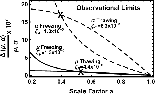
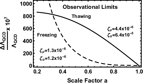
This shows that the observationally constrained change in is limited to a factor of between a scale factor of 0.4 and 1.0 for both the freezing and thawing cases. At a scale factor of 0.2 the freezing cosmology change can be on the order of while the thawing change is limited to .
7.2 Model Constrained Evolution
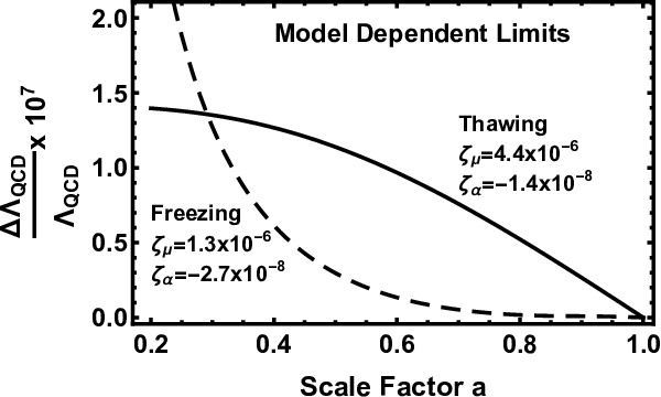
Figure 4 shows that the model constrained limit on is significantly reduced by a factor of relative to the evolution. As shown in Fig. 5 the model constrained case predicts very little evolution with changes in limited to between a scale factor of 0.2 and the present scale factor of 1. A scale factor of 0.2 is a redshift of 4.0 and a look back time of approximately 11.5 gigayears.

7.3 Limits on the current rate of change of
The integrand in (27) is the derivative of or with respect to the natural log of the scale factor . Multiplying this by the Hubble Constant converts the integrand to a time derivative. The current rates of change of and are then just the integrand at a scale factor of 1 multiplied by the current value of H, H0.
| Limits | Cos. | |||||
|---|---|---|---|---|---|---|
| Obs. Limits | Frz. | 9.3E-17 | 8.9E-18 | 4.1E-15 | 4.1E-15 | 2.6E-17 |
| Thw. | 2.7E-16 | 1.9E-17 | 1.2E-14 | 1.2E-14 | 7.6E-17 | |
| Mod. Limits | Frz. | 1.9E-19 | 8.9E-18 | -1.2E-17 | -2.4E-17 | -1.5E-19 |
| Thw. | -5.9E-19 | 1.9E-17 | -9.7E-18 | -3.4E-17 | -2.1E-19 | |
| Lab | - | 2.1E-17 | 1.1E-16 | - | - | - |
Table 2 gives the limits on the current rates of change per year of the constants and parameters for the freezing and thawing cosmologies under the observational and model dependent limits. The physics parameter rates of change per year, , and are clearly too small to measure on laboratory time scales. The observational limit on is not as restrictive as the current laboratory limits but the model dependent limit is two orders of magnitude more restrictive. For the observational limits are an order of magnitude more restrictive than the laboratory results. As expected the thawing cosmologies allow a higher present day rate of change of the constants and the parameters than the freezing cosmology which has a lower present day rate of change than the thawing cosmology. This shows the dangers of using a linear rate of change between the astronomically observed limits and the present day to predict the current rates of change.
8 Future Observations
Optical astronomical observations with high spectral resolution spectrometers on current and future large telescopes may have the best chance of improving the limits the time evolution of the physical parameters. This is particularly true at high redshift where the radio observations have yet to be accomplished. The radio observations at low redshift may have reached the limit where thermal and bulk motions of the absorbing gas could prevent more accurate constraints. The highest existing or planned spectral resolution optical spectrometer is the PEPSI instrument (R=300,000) recently installed on the Large Binocular Telescope. The spectrometer is currently undergoing commissioning and has the potential for significant improvement over previous observations. The currently executing Large Program on the VLT (Molaro et al., 2013) also has great potential where the emphasis is on reducing the systematic errors in wavelength calibration through controlled observation programs and new calibration techniques as well as increasing the number of observations. It is key in checking the claims of a variation in .
9 Conclusions
Measurements of the stability of the fundamental constants in the early universe provide an important tool for the evaluation of new physics and cosmologies that predict time variation of the basic physics parameters that determine the value of the constants. In particular the combination of the observational limits on the time variation of the proton to electron mass ratio and the fine structure constant limit the fractional change of the Quantum Chromodynamic Scale and the sum of the fractional changes of the Higgs Vacuum Expectation Value and the Yukawa couplings in terms of the model dependent parameters and . For the well known model of Coc et al. (2007) where and the limit on the fractional change of the QCD scale and the sum of the fractional changes of the Higgs VEV and the Yukawa couplings is at the level for the last half of the age of the universe. Further introduction of the model dependent parameter in the relation provides individual limits on a variation of the Higgs VEV and the Yukawa couplings.
The direct connection between the fundamental constants and the physics parameters provides a mechanism to limit the time evolution of the parameters for rolling scalar field cosmologies. The variation of and with time or scale factor is related to the evolution of the dark energy density and the the dark energy equation of state (Calabrese et al., 2011; Thompson, 2012). The QCD Scale as a function of the scale factor in slow roll quintessence is examined as an example of such evolution. A primary conclusion of the work is that the fundamental constants play a central role in examining the validity of new physics and alternative cosmologies by defining the parameter space of the theories that is consistent with observed limits on variability of the constants.
References
- Aad et al. (2012) Aad, G. et al. 2012 Physics Letters B, 716, 1
- Abbott et al. (2016) Abbott, B.P. et al. 2016, Phys. Rev. Lett., 116, 061102
- Bagdonaite et al. (2013) Bagdonaite, J.,Dapra, ¡ Jansen, P., Bethlem, H.L., Ubachs, W., Henkel, C., & Menten, K.M. 2013, Phys. Rev. Letters, 111, 231101
- Calabrese et al. (2011) Calabrese, E., Menegoni, E., M., Martins, C.J.A.P., Melchiorri, A. & Rocha, G. 2011, Phys., Rev. D, 84, 023518
- Calmet and Fritzsch (2002) Calmet, X. and Fritzsch, H. 2002, Phys. Lett. B, 540, 173
- Campbell and Olive (1995) Campbell, B.A. and Olive, K.A. 1995, Phys. Lett. B, 345, 429
- Chamoun et al. (2007) Chamoun, N., Landou, S.J., Mosquera, M.E. and Vucetich, H. 2007, J. Phys. G: Nucl. Part. Phys., 34, 163
- Chatrchyan, S. et al. (2012) Chatrchyan, S. et al. 2012 Physics Letters B, 716, 30
- Coc et al. (2007) Coc, A., Nunes, N.J., Olive, K.A., Uzan, J-P, & Vangioni, E. 2007, Phys. Rev. D, 76, 023511
- Dent (2008) Dent, T. 2008, Eur. Phys. J. Special Topics 163, 297–313
- Dine et al. (2003) Dine, M., Nir, Y., Raz, G. and Volansky, T. 2003, Phys. Rev. D, 67, 015009
- Dutta & Scherrer (2011) Dutta, S. & Scherrer, R.J., Phys. Lett. B, 704, 265
- Flambaum and Kozlov (2007) Flambaum, V.V. and Kozlov, M.G. 2007, Phys. Rev. Let., 98, 240801
- Godum et al. (2014) Godum, R.M., Nisbet-Jones, P.B.R., Jones, J.M., King, S.A., Johnson, L.A.M., Margolis, H.S., Szymaniec, K., Lea, S.N., Bongs, K. & Gill, P. 2014, Phys. Rev. Lett., 113, 210801
- Jansen et al. (2011) Jansen, P., Xu, L.H., Kleiner, I., Ubachs, W., and Bethlem, H. L., Phys. Rev. Let. 2011, 106, 100801
- Kanekar et al. (2015) Kanekar, N., Ubachs, W., Menten, K.M., Bagdonaite, J., Brunthaler, A., Henkel, Muller, C.S., Bethlem, H.L. and Dapra, M. 2015, MNRAS 448, L104
- King et al. (2011) King, J. A., Webb, J. K., Murphy, M., Ubachs, W, & Webb, J. 2011, MNRAS, 417, 3010
- Langacker et al. (2002) Langacker, P., Segre, G. and Strassler, M.J. 2002, Phys. Lett. B, 528, 121
- Langacker (2004) Langacker, P. 2004, Int. Jr. Mod. Phys. A, 19, 157
- Levshakov et al. (2011) Levshakov, S.A., Kozlov, M.G. and Reimers, D. 2011, Ap.J., 738, 26
- Molaro et al. (2013) Molaro et al. 2013, A&A, 555, A68
- Murphy et al. (2016) Murphy, M.T., Malec, A. and Prochaska, J.X. 2016, MNRAS 461, 2461
- Thompson (1975) Thompson, R.I. 1975, Astrophys. Lett., 15, 3
- Thompson (2012) Thompson, R.I., 2012, MNRAS Letters, 422, L67
- Thompson (2016) Thompson, R.I., 2016, Proceedings of the 14th Marcel Grossmann Conference arXiv:1602.03192v1 [astro-ph.CO]
- Uzan (2011) Uzan, J-P 2011, Living Rev. Relativity, 14, 2
- Webb et al. (2001) Webb, J.K., King, Murphy, M.T., Flambaum, V.V., Dzuba, V.A., Barrow, J.D., Churchill, C.W., Prochaska, J.X. & Wolfe, A.M. 2001, PRL, 87, 091301-1-4
- Webb et al. (2011) Webb, J.K., J.A., Murphy, M.T., Flambaum, V.V., Carswell, R.F., & Bainbridge, M.B. 2011, PRL, 107, 191101-1-5