Effects of magnetic fields on quark-antiquark interactions
Abstract:
We discuss some recent results obtained in the study of strong quark-antiquark interactions in the presence of intense external magnetic fields by means of lattice QCD simulations. We confirm previous findings and show that both at zero and finite temperature the external field induces anisotropies in the static quark potential. An in-depth study suggests that the effects are essentially due to the variation of the string tension whose angular dependence can be nicely parametrized by the first allowed term in a Fourier expansion. In the confined phase at high temperature, we observe that the suppression of the string tension is enhanced as the strength of the external field increases. Our results support the idea that the loss of confining properties is the dominant effect related to the decrease of as a function of .
24-30 July 2016
University of Southampton, UK
1 Introduction
In many situations, such as heavy ion collisions [1] or in the early Universe [2], large magnetic fields with intensities of are produced and affect the properties of strongly interacting matter. In these contexts, the magnetic fields may lead to significant modifications of the properties of QCD. Indeed, even if gluons are not directly coupled to electro-magnetic fields, substantial contributions can arise from quark loops. This is confirmed both by analytical studies that use effective field theories or perturbation theory and by many evidences from lattice investigations (see, e.g., Refs. [3, 4] for general reviews).
Important modifications may be expected on the static potential between heavy quarks. In the explorative study in Ref. [5] it has been found that both the Coulomb term and the linear confining piece of the potential become anisotropic when a strong external magnetic field is turned on. This has also been predicted by several model studies and could have phenomenologically relevant effects in the heavy meson spectrum and production in heavy ion collision [6, 7, 8, 9, 10]. In our study we carry on the investigation of these effects on the potential at zero temperature and explore also the confined phase in the finite temperature regime. At , a quantitative description of the behaviour of the string tension and of its angular dependence is provided, together with hints about its fate in the large field limit. Then we move to the exploration of the regime, in order to check whether the anisotropic effect survives, and also to investigate the role of the magnetic field in the string tension suppression near the deconfinement transition.
2 Numerical setup
In our work we consider QCD with quark flavours discretized using a Symanzik tree-level improved gauge action and stout improved rooted staggered fermions. The partition function reads
| (1) |
where is the measure over the gauge link variables, is the gauge action [11, 12] involving the real part of the traces over and loops and is the staggered fermion matrix with two-times stout-smeared gauge links [13].
In order to consider the effect of an external background magnetic field, in the continuum we introduce the abelian gauge four-potential into the quark covariant derivative which takes the form with electric charge related to the quark flavour . In the discretized theory, where this operator is written in terms of the SU(3) gauge links (with lattice site and direction), the insertion of the electromagnetic field corresponds to the substitution where is a U(1) phase related to . We consider external fields, hence is non-propagating: no kinetic term is added to the Lagrangian.
In our case we work with a constant and uniform magnetic field [3]. If we choose to fix along one of the lattice axes (say ) then it is possible to show that, due to the lattice periodic boundary conditions, the quantization condition with must hold, where is the electric charge unity and and are the lattice extents along and . If is not aligned along one of the axes, we can consider each component separately and write the total abelian phase as the product of them over the three axes [14]. Each component of must satisfy an independent quantization condition and will be associated to an integer vector . If the magnetic field vector is proportional to .
We performed simulations at physical quark masses, i.e. tuning the parameters according to the line of constant physics reported in Refs. [15, 16]. Note that the presence of the external field does not affect the lattice spacing [17]. At zero temperature we used four lattices , , and with spacings ranging from to , and for each of them, we performed runs with magnetic field quanta up to ; this give us access to fields roughly up to . For we used lattices with and , corresponding to physical temperatures sligthly below . In all cases, gauge configurations have been sampled by the Rational Hybrid Monte-Carlo algorithm [18], collecting statistics of the order of trajectories for each value of .
At , the static potential is extracted from planar Wilson loops. Note that loops oriented along different directions cannot generically be averaged since the rotational symmetry is broken to by the external magnetic field. At finite , instead, we extracted the free energy of a quark-antiquark pair from Polyakov loop correlators.
3 Analysis and results
We adopted the following strategy: first, we determined the values of the potential parameter at and in order to use them as a reference for the subsequent analysis. Then we investigated the influence of the external field, performing a continuum limit extrapolation of all the relevant observables. Finally, we moved on to the regime, by working on our finest lattice to investigate whether the anisotropies survive.
3.1 T=0
It is known that the potential can be well described by the Cornell parametrization [19]
| (2) |
where is the Coulomb term, is the so-called string tension and is a constant. This functional form fits very well our data at and with parameters11 1 The statistical error is obtained from the fit of our data (the largest lattice spacing has been discarded); the systematic uncertainty has been estimated by using also the fit model. and , that will be used as reference in the following, corresponding to a value of the Sommer parameter [20] .
Turning the magnetic field on, we expect the potential to become anisotropic and to acquire different values in the directions orthogonal or parallel to [5]. In general, one can promote the potential to a function of the magnetic field and of the angle between and the orientation. This general parametrization takes into account the residual cylindrical symmetry around ; we will also impose symmetry under the reflection . Then, assuming the potential to be of the Cornell form (2) for all values of , the most general form of compatible with these symmetries is
| (3) |
where the potential parameters bring all the dependence on .
In order to verify the reliability of this model, we analyzed the angular dependence of the static potential on our two finest lattices (corresponding to the lattice sizes and ) for three different orientations of the magnetic field with , giving us access to 8 different angles. Results are shown in Fig. 1.
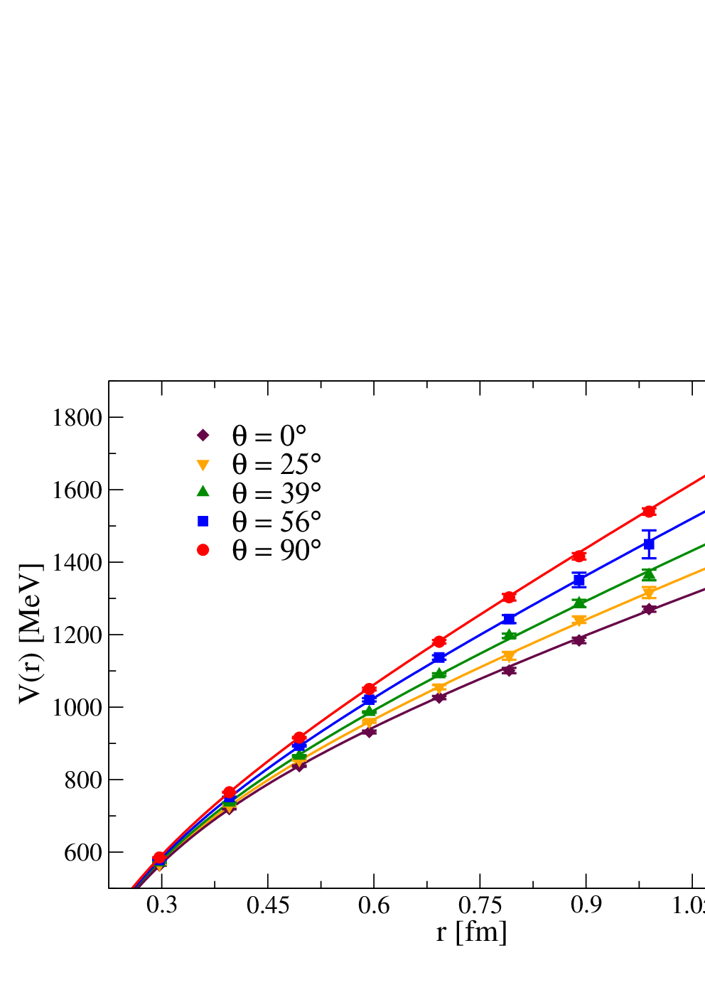

As expected from the preliminary data in Ref. [5], the potential increases with the angle, and the model in Eq. (3) fits very well our data. We found that the values , which are a sort of average of the parameters over the angles, are all compatible with those at . Morover, it turns out that it is sufficient to consider only the first terms in the Fourier series22 2 If successive terms with are included in the fit model, they turn out to be all compatible with zero., as show in Fig. 1.
We performed a continuum limit extrapolation to determine whether these anisotropies are only lattice artifacts or truly physical effects. A complete determination of the angular distributions and of the dependence would require many simulations with different lattice spacings and several values and orientations of the magnetic field. However, since only the s terms are needed in the description of the angular dependence (at least with our precision), we can simplify the task considerably by considering the two quantities
| (4) |
These are, respectively, the anisotropy and the average value of the parameter taken along the and directions. Using the fact that when , it is easy to show that and . Therefore, we can access all the information about the anisotropies just by measuring the potential in the directions parallel or orthogonal to the magnetic field.
Results for the anisotropies of and , together with their continuum limit extrapolations, are shown in Fig. 2.


The fit procedure has been performed using a general power law for the coefficients as a function of , with corrections, and it gave us very good values of the test [14]. In the case of the string tension, the anisotropy survives in the continuum limit and grows with the magnetic field. Conversely, the continuum limit of is compatible with zero, like for [14]. We can therefore conclude that the effect of the magnetic field on the static potential persists in the continuum limit and is mostly due to the variation of the string tension.
Finally, our findings suggest a sort of anisotropic deconfinement at very large magnetic fields (see Fig. 3).

Indeed, for the string tension is predicted to vanish in the longitudinal direction by extrapolating our fit results. Data obtained for large seem to roughly agree with this behaviour, however a precise continuum extrapolation is difficult in this region due to large cut-off effects expected at . By now, the presence of this sort of critical value of is to be taken as a fascinating speculation.
3.2 T¿0
Results for the free energy of a static pair at temperatures lower than are shown in Fig. 4.


As one can see, the potential roughly follows the same behaviour observed in the case, with the anisotropy still present. In this temperature regime, the dominant effect turns out to be the flattening of the potential as is increased. As a result, the Cornell form in Eq. (2) ceases being suitable for the description of the potential when both the temperature and the magnetic field grow. This can be also seen from the behaviour of string tension (leftmost plot in Fig. 5): as expected, tends to vanish as reaches the pseudocritical temperature , but this effect is remarkably enhanced by the presence of the magnetic field.


These results are consistent with the picture of a decreasing chiral pseudocritical temperature shown in previous studies [17, 21]. In the so-called inverse magnetic catalysis, the decrease of is responsable of the non-monotonic behaviour of the chiral condensate near the transition temperature. Our data gives us evidences of the same phenomenon at the level of the confining properties. Morover, the latter seems to be dominant effect: in the range of and explored (see right plot Fig. 5), the inverse magnetic catalysis is hardly noticeable, while the flattening of the potential is clearly visible.
4 Conclusions
It has been confirmed that the static potential is strongly affected by an external magnetic field, becoming anisotropic. Studying its angular dependence and performing continuum extrapolations at we have shown that the anisotropy is a physical effect that persists in the continuum limit. This is mostly due to the variation of the string tension, whose angular dependence is very well described by just the first Fourier term . In the high-temperature regime, the anisotropy is reduced and the main effect of the magnetic field is the precocious disappeareance of the confining properties, indicated by the flattening of the potential at large distances and by the vanishing of the string tension, something that can be called deconfinement catalysis. This phenomenon can be understood in terms of a decreasing and is noticeable even at low values of the magnetic field, when there are no signals of inverse magnetic catalysis in the chiral condensate.
Acknowledgments.
We acknowledge PRACE for giving us access to FERMI machine at CINECA in Italy, under project Pra09-2400 - SISMAF. FS received funding from the European Research Council of the European Community Seventh Framework Programme (FP7/2007-2013) ERC grant agreement No 279757. FN acknowledges financial support from the INFN project SUMA.References
- [1] V. Skokov, A. Y. Illarionov and V. Toneev, Int. J. Mod. Phys. A 24, 5925 (2009) [nucl-th/0907.1396].
- [2] T. Vachaspati, Phys. Lett. B 265 (1991) 258.
- [3] D. E. Kharzeev, K. Landsteiner, A. Schmitt and H. U. Yee, Lect. Notes Phys. 871, 1 (2013).
- [4] V. A. Miransky and I. A. Shovkovy, Phys. Rept. 576, 1 (2015) [hep-ph/1503.00732].
- [5] C. Bonati et al., Phys. Rev. D 89, 114502 (2014) [hep-lat/1403.6094].
- [6] K. Hattori, T. Kojo and N. Su, Nucl. Phys. A 951, 1 (2016) [hep-ph/1512.07361].
- [7] X. Guo, S. Shi, N. Xu, Z. Xu and P. Zhuang, Phys. Lett. B 751, 215 (2015) [hep-ph/1502.04407].
- [8] K. Fukushima, K. Hattori, H. U. Yee and Y. Yin, Phys. Rev. D 93, 074028 (2016) [hep-ph/1512.03689].
- [9] P. Gubler et al. Phys. Rev. D 93, 054026 (2016) [hep-ph/1512.08864].
- [10] C. Bonati, M. D’Elia and A. Rucci, Phys. Rev. D 92, 054014 (2015) [hep-ph/1506.07890].
- [11] P. Weisz, Nucl. Phys. B 212, 1 (1983).
- [12] G. Curci, P. Menotti and G. Paffuti, Phys. Lett. B 130, 205 (1983)
- [13] C. Morningstar and M. J. Peardon, Phys. Rev. D 69, 054501 (2004) [hep-lat/0311018].
- [14] C. Bonati et al., Phys. Rev. D 94 (2016) 094007 [hep-lat/1607.08160].
- [15] Y. Aoki et al., JHEP 0906, 088 (2009) [hep-lat/0903.4155].
- [16] S. Borsanyi et al., JHEP 1011, 077 (2010) [hep-lat/1007.2580].
- [17] G. S. Bali et al., JHEP 1202, 044 (2012) [hep-lat/1111.4956 [hep-lat]].
- [18] M. A. Clark and A. D. Kennedy, Phys. Rev. D 75, 011502 (2007) [hep-lat/0610047].
- [19] E. Eichten et al., Phys. Rev. Lett. 34, 369 (1975).
- [20] R. Sommer, Nucl. Phys. B 411, 839 (1994) [hep-lat/9310022].
- [21] G. S. Bali et al., Phys. Rev. D 86, 071502 (2012) [hep-lat/1206.4205].