Optimal control for perfect state transfer in linear quantum memory
Abstract
A quantum memory is a system that enables transfer, storage, and retrieval of optical quantum states by ON/OFF switching of the control signal in each stages of the memory. In particular, it is known that, for perfect transfer of a single-photon state, appropriate shaping of the input pulse is required. However, in general, such a desirable pulse shape has a complicated form, which would be hard to generate in practice. In this paper, for a wide class of linear quantum memory systems, we develop a method that reduces the complexity of the input pulse shape of a single-photon while maintaining the perfect state transfer. The key idea is twofold; (i) the control signal is allowed to vary continuously in time to introduce an additional degree of freedom, and then (ii) an optimal control problem is formulated to design a simple-formed input pulse and the corresponding control signal. Numerical simulations are conducted for -type atomic media and a networked atomic ensembles, to show the effectiveness of the proposed method.
1 Introduction
Photons, due to its nature of low interaction with the environment, is the most popular candidate of an information carrier for secure quantum communication. The technology of light transmission has been well developed, which raises its popularity. However, because a photon is not well suited for local manipulation, a photonic state must be converted to a stationary state of a solid system for storage and information processing [1]. In fact, various methods for such a state conversion have been studied [2, 3, 4, 5]. In particular, the electromagnetic induced transparency (EIT) effect can be employed to switch the couplings between the metastable states of atoms and an optical field to preserve the state once the photon has been absorbed into the atoms [6]. We refer to Refs. [7, 8] for reviewing the recent progress of optical quantum memory.
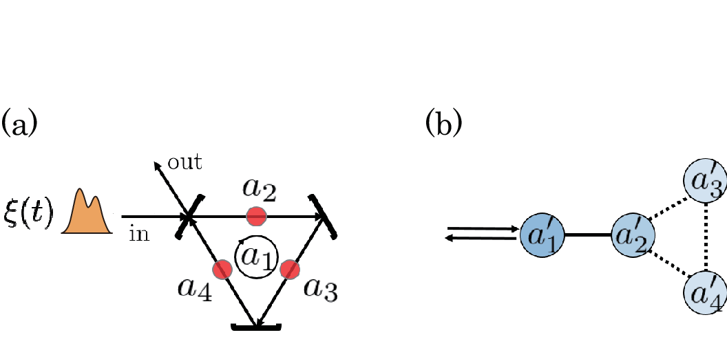
Now let us consider the general configuration of a quantum memory system. As illustrated in Fig. 1, it consists of two subsystems: the buffer subsystem and the memory subsystem. The buffer subsystem is coupled to both the external field and the memory subsystem, while the memory subsystem is only coupled to the buffer subsystem. The interaction between the two subsystems can be controlled by an ON/OFF switching signal so that the quantum state is preserved inside the memory subsystem once all the state is fed into it. Given a physical system having the above configuration, then the problem is how to design an efficient or even optimal transfer, storage, and retrieval processes. For instance, for an atomic quantum memory incorporating the EIT effect, we find some methods that compute a time-varying control signal achieving optimal state transfer, based on the information gained from the leaking output [9, 10, 11, 12, 13]. Also, for a wide class of open quantum systems, i.e., passive linear quantum systems such as a large atomic ensemble and an opto-mechanical crystal array [4, 11, 14, 15], the general procedure for achieving a perfect state transfer was developed [16]; in particular, it was found that the pulse shape of an input photon, , must be the generalized rising-exponential function to accomplish the perfect state transfer if the ON signal takes a constant value. However, it is often the case that a generalized rising-exponential function has a complicated form, and experimental implementation of such a complex pulse shaping of a single photon field is a challenging task. In fact, even in the case of generating a simple rising exponential such as , we need to elaborate a sophisticated photon generator based on a cold atomic media [17, 18, 19, 20] or an asymmetric optical parametric oscillator [21]. Extension of these schemes to the general multi-mode setup must be more involved and challenging.

The contribution of this paper is to solve the above mentioned issue; that is, for a general passive linear quantum system having the configuration shown in Fig. 1, we develop an optimal control theory for computing a low-complexity pulse function of an input single-photon that can be perfectly absorbed into the memory subsystem, by employing a time-varying control signal . This idea is based on the fact that, in contrast to the difficulty for shaping a complex pulse function of a single-photon field in an experiment, there are many setups where even a complicated and fast control signal can be easily implemented using a laser pulse shaping; this fact has been demonstrated in the field of quantum (open-loop) optimal control [22, 23]. That is, our method can be used to make the perfect state transfer protocol more feasible, by converting the complexity of (hard to implement) to that of (easy to implement compared to ). Note that a similar approach, but for a concrete example, was developed in [9, 10, 11, 12, 13]; a remarkable difference of these works to our approach is that in their setup the input pulse function is given and then the optimal control maximizing the storage efficiency is computed; note thus that, in this setup, the state transfer is in general not perfect. Meanwhile, in our case, both the optimal pulse function and the optimal control signal can be found out of many combinations of those, in such a way that the perfect state transfer is guaranteed.
This paper is organized as follows. Section 2 presents the general model analyzed throughout the paper and introduces the dynamical equations for the single-photon pulse function. In Section 3, we derive the general condition for the pulse function and the control signal to achieve the perfect state transfer. Section 4 begins with the formulation of optimal control problem and then presents two examples, -type atomic media and a networked atomic ensembles system. A concrete algorithm for solving the optimal control problem is given in Appendix B.
Notations: For a matrix , the symbols , , and represent its Hermitian conjugate, transpose, and complex conjugation in elements of , respectively; i.e., , , and . For a matrix of operators we use the same notation, in which case denotes the adjoint to . For a time-dependent variable , we denote .
2 Preliminaries
2.1 Passive linear quantum systems
In this work, we follow the same model presented in [16], the general passive linear quantum system [4, 11, 14, 15]. This is an open quantum system composed of harmonic oscillators represented by a vector of annihilation operators , satisfying the commutation relation . The system interacts with a single external optical field, whose annihilation process is denoted by the operator , satisfying . The system has a time-varying Hamiltonian of the form , where is an Hermitian matrix. Further, the system-field instantaneous coupling is represented by , where is a -dimensional complex row vector. Then from the input-output formalism [24], the Heisenberg dynamics of the system variable, with the joint unitary evolution of the system and the field, together with the change of the field operator, is given by:
| (1) |
where and is the annihilation process operator of the output field. Note that the vector can be time-varying, but in this paper it is assumed to be time-invariant.
2.2 Single photon field
The annihilation operator for the continuous-mode single-photon state is defined by
| (2) |
where is a -valued pulse shape function satisfying the normalization condition (thus have the meaning of a probability distribution). A single photon field state is defined as
| (3) |
where denotes the field vacuum state. As expected, the operator annihilates the photon; . Note that the method proposed in this paper also functions for the case when the input is given by a pulsed coherent field state. However, for a coherent field state, even a complex wave packet can be effectively generated by an electro-optic modulator, and thus our method may not need to be applied in this case.
2.3 Dynamics of the pulse shape and the statistics
In this paper, the input field state for the system (1) is given by the single photon field state (3). The system’s initial state, at time , is assumed to be the ground state . Thus, the initial state of the whole system is . Then, due to the passivity property, the system’s output state on the field is also a single photon state; let be the pulse function of this output single photon state. In this setup, the input pulse shape and the output pulse shape are connected by the following classical differential equation having the same form as that of Eq. (1) [16, 25, 26]:
| (4) |
The derivation of this equation is given in Appendix A; in particular, the definition of the -valued vector is given in Eq. (59). At time when the perfect state transfer is achieved, coincides with the superposition coefficients of the system state (see Appendix A); this will be used as a terminal condition of the optimization problem formulated in Section 4. Note that, if the input is a coherent field state with amplitude , we have the same input-output relationship as above, in which case stands for the vector of means of the system coherent state.
Next let us define the correlation matrix as , whose diagonal terms represent the mean photon number in each mode. The dynamics of is given by
| (5) |
where obeys Eq. (4).
3 Condition for perfect state transfer
3.1 Linear quantum memory system
Throughout this paper, we consider a particular class of passive linear quantum systems which has the ability for transfer, storage, and retrieval of a quantum state. We let the system to have three components , where is a single annihilation operator, and and are vectors of and annihilation operators, respectively. Then the Hamiltonian matrix is given by , where
are time-invariant matrices and is a control signal which modulates the Hamiltonian. The size of the matrices and is , where we have defined . We also define with . Hence, Eq. (1) is now given by
| (26) | |||||
It is immediate to see that, during , the second mode entirely decouples from the input field and the other system modes. Therefore, functions as a memory subsystem, because once the photon is transferred into the state of , that state can be preserved for a long time by tuning . The other modes and are the buffer subsystems, which mediate the state transfer from the optical field to the memory subsystem. The relation of the three groups of modes is illustrated in Fig. 2. Finally note that the input and output pulse functions and are connected by Eq. (4), which is now

3.2 Zero-dynamics principle for perfect state transfer
For the perfect transfer of a photonic state, the output pulse function must always be zero during the state transfer process; this is the idea of zero-dynamics principle for perfect state transfer [16]. Thus, from Eq. (4), the condition we desire is . The time derivative of the output pulse is then calculated as
which is also zero since the output must be constantly zero. Substituting the zero-output condition for the above equation, we have
| (28) |
This equation can be simply represented as
| (29) |
where and are fixed matrices. Let us next derive the boundary condition from the system’s final state when the state transfer is accomplished at time . First, since coincides with the terminal superposition coefficients of , we have and for the perfect state transfer into the memory subsystem. Also from , the input pulse must satisfy . In total, . The dynamics (28) or (29) with this boundary condition is called the zero-dynamics, and it can be uniquely solved backwards in time starting from once is specified. In other words, this dynamics is the condition imposed on and for achieving the perfect state transfer.
3.3 Constant control and rising exponential function
Let us consider the special case when the control signal is constant. In this case, letting in Eq. (4) readily yields
| (30) |
where is a Heaviside step function taking for and for . Note of course that Eq. (30) is the solution of Eq. (28) when is constant.
To see explicitly a feature of the function (30), let us consider a single-mode system specified by and ; the dynamical equation of the system annihilation operator is given by
Typically, this system can be implemented as an optical cavity coupled to an external field, where is proportional to the transmissivity of the coupling mirror. In this case, Eq. (30) is given by , where is assumed for simplicity. That is, the pulse function is of the rising exponential form 11 1 A single-photon field state with this pulse function can be perfectly absorbed into the cavity. Note however that, if we want to use this system as a memory device, the coupling strength has to be a controllable time-varying parameter; that is, must be changed to zero immediately after the state transfer is finished. . Based on this observation, we call Eq. (30) the generalized rising exponential function, for systems with the number of modes more than or equal to two. In fact, in terms of the eigenvalues of , , Eq. (30) can be represented as with the constant coefficients; hence, under the assumption that , which is required to achieve the perfect state transfer [16], Eq. (30) is indeed the sum of rising exponential functions. Note again that a single-photon field state over the pulse function (30) is perfectly absorbed into the corresponding multi-mode passive linear system (1). Also we remark that Eq. (30) is the time-reversed version of the system’s output field [16], as in the single-mode case [27, 28]. However, as we refer in the examples in the next section, a generalized rising exponential function has a complicated form in general; thus realization of a single-photon field state with such a complex pulse function is still a challenging task, while, as mentioned in Section 1, a simple rising exponential of a single-photon field state is possible to experimentally generate, using current technology.
4 Optimal control for quantum memory
The main purpose for considering the variation of the control signal is to reduce the complexity of the pulse function (30), while maintaining the perfect state transfer. The problem is that, as implied by Eq. (28), there are infinitely many combinations of and that satisfy the condition for perfect state transfer. In this section, we present an optimal-control formulation for determining the optimal pair of low-complexity pulse function and the corresponding control signal, and then show two examples.
4.1 Designing the cost function
As mentioned above, the general rising-exponential pulse function of a single-photon is often of a very complicated form, which would be hard to generate. On the other hand, a single-photon field traveling with a simple rising exponential pulse function such as shown above can be experimentally generated [17, 18, 19, 20, 21], although such a simple function cannot perfectly transfer the photon into the memory subsystem 22 2 From Eq. (28) and the boundary condition, the time derivative of the pulse function at time is . Thus, the simple rising exponential function does not transfer the state into the memory subsystem perfectly, except the case where the system is a single-mode system; see the footnote in Page 6. . Therefore, as a compromise, we consider a unimodal function; that is, here we formulate an optimal control problem such that the cost function is minimized when the pulse function takes a unimodal form. This policy is supported by the fact that a source system generating a single photon with unimodal pulse function has been experimentally implemented in several setups, such as cavity QED [29, 30, 31], ion trap [32], circuit QED [33], and cold atoms [34, 35]. Actually, by properly modulating the source system during the photon emission process, we can flexibly tailor the pulse shape so that the desired unimodal pulse function is realized. For instance, it was demonstrated in the ion-trap setup in [32] that the duration of the Gaussian-shaped pulse of the emitted single photon can be controlled by tuning the intensity of the driving field for the ion; also, the circuit-QED-based scheme developed in [33] generates a single photon with various -shaped form, by a proper modulation of the driving microwave signal that effectively changes the qubit-resonator coupling.

According to the above-described policy, we define a cost function so that would monotonically increase until it meets its single extremum and decrease after the pulse reaches that extremum. Let be the time of this extremum; hence . Then, the cost function should impose a penalty when the pulse function is not increasing until and not decreasing after . A simple optimal control problem satisfying this policy can be defined as
where
for a dimensionless constant . Actually this cost function takes a smaller value if for and for ; Fig. 3 illustrates the relation between , , and in this desired case. Note that is a decision variable. Also the constraint of this optimization problem is given by Eq. (29), which together with the boundary condition is
The above optimal control problem can be generalized to
| (33) |
where is an increasing function introduced to enhance the penalty. In particular, we set . Moreover, the cost over the control sequence and the boundary condition should be also taken into account. Thus, the overall cost function is given by
| (34) |
Here, are dimensionless positive constants that change the weight of each cost. Summarizing, the optimal control problem is to find that minimizes the cost (34) under the constraint (4.1). Because the variable is fixed at the terminal time , this optimization problem is solved backwards in time; the initial time is chosen so that the initial system state is enough close to the ground state, or equivalently that the initial variable is enough close to zero. The detailed procedure for calculating the optimal pair of and is given in Appendix B.
4.2 -type atomic media

In this section, we study a -type atomic ensemble trapped in an optical cavity, investigated in [9, 10, 11, 12, 13]. In this model, there are atoms with three energy states as shown in Fig. 4 (a), where the transition of frequency couples to the cavity radiation mode with frequency , and the transition of frequency couples to an external control field with frequency having a time-varying Rabi frequency envelope . The system variables are the polarization operator , the spin-wave operator ( are collective atomic operators for ), and the cavity mode operator . When , the operators and can be approximated as annihilation operators, and the Heisenberg equation of is given by
where is a coupling constant between the atoms and the cavity field. Also denotes the detuning, which is assumed to be zero for simplicity. The cavity decay rate is , so the relation between the input process operator and the output correspondence is given by
| (35) |
Now defining and , the above equations can be represented in the form of passive linear quantum system (1) with system matrices
and the system variables . That is, functions as the buffer subsystem and does the memory subsystem, as illustrated in Fig. 4 (b); actually when , the spin-wave mode is decoupled from the other modes and the field mode . Note that the parameters defined in Eq. (26) are , , , , , and .

Now the objective is to transfer a single-photon to the spin-wave mode , implying that the final state is set to . The pair of optimal low-complexity input pulse function and the corresponding control signal , which achieves the perfect state transfer, can be computed by solving the optimal control problem developed in the previous subsection; more precisely, as described in Appendix B, the gradient method [39, 40] combined with the Euler-Lagrange equations (64), (65), and (66) subject to the dynamics (5.1) and the cost function (34) yields the optimal solution. The system parameters are chosen so that . Also the dimensionless weighting parameters are set to ; the reason of choosing a large value of is to strongly impose the initial variable to be close to zero.
Figure 5 (a) shows the absolute value of pulse function (probability density), i.e., with and . The dashed blue line represents the generalized rising exponential function (30) corresponding to the constant control , and the solid red line shows the optimized pulse function corresponding to the optimal time-varying control signal ; these control signals are illustrated in Fig. 5 (b). A remarkable fact is that, in contrast to the complicated pulse shape realized with the constant control, the optimized pulse function has a simple unimodal shape with extremum point , thanks to the aid of optimal time-varying control signal. As discussed in Section 4.1, implementing this unimodal pulse of a single photon may be feasible with current technology. Also, the phase of the single-photon pulse is fixed to for all , implying that the phase modulation of the single-photon field is unnecessary.
Note that this time-varying signal looks complicated as well, but the external optical field with this level of frequency envelope is feasible to implement, as shown in the experiment [12, 13]; recall that, on the other hand, implementing the complex pulse shape corresponding to the constant control may be a challenging task.
Finally let us confirm that the perfect state transfer is achieved. Figure 6 shows the time evolution of the mean photon numbers inside the atomic medium, i.e., , which can be calculated using Eq. (5). We then actually observe that the photon has been transferred into the memory subsystem mode at the final time , while the buffer subsystem is excited during the time-evolution but finally decays to the ground states.

4.3 Network of atomic ensembles
First of all, let us remember the fact that the optimization problem formulated in Section 4.1 does not necessarily yields a unimodal pulse function as the optimal solution. Hence, it should be worth investigating to see if a unimodal input pulse function could be obtained for a more complicated system than the previous -type atomic media where actually the optimal solution is given by a unimodal function. In this subsection, we study a networked system composed of large atomic ensembles and an optical cavity field, provided in [16, 36, 37, 38]; in fact, as will be shown later, this system forms a target memory subsystem in a nontrivial way, unlike the previous example.
The configuration of the system is shown in Fig. 7 (a). The network contains three atomic ensembles; the th ensemble couples to the common single cavity mode through external pulse lasers with Rabi frequencies and . The coupling Hamiltonian is given by
| (36) |
where is the bosonic annihilation operator approximating the atomic collective lowering operators in the large ensemble limit. Also, is the laser phase, is the number of atoms in each ensemble, is the coupling strength, and is the detuning. The spontaneous emission of each atom is negligible for typical atoms such as 87Rb. Moreover, for the second and third ensembles, the ground state is coupled to the excited state, through another controllable laser field with Rabi frequency . This effect can be represented by the Hamiltonian ; note that this is the sum of local Hamiltonians acting on each atomic ensemble. We set the parameters as and for , and define . As a result, the whole system Hamiltonian is given by
The cavity mode interacts with an external light field at the partially reflective mirror, via the Hamiltonian . Summarizing, the system is a passive linear quantum system with the following system matrices:
Now let us define the unitary matrix
which transforms the system equations to
where
This equator clearly shows that corresponds to the buffer subsystems and does the memory subsystems; once the photon is transferred to the memory subsystem, then by setting the control signal to , the state can be preserved. A striking feature of this system is that the buffer-memory interaction can be regulated by the local control on the second and third ensembles.

Here we set the goal to transfer a single-photon into the mode , implying that the terminal condition is given by . The parameters are chosen so that . Also the dimensionless weighting parameters are chosen as ; thus, the penalty on the control is taken to be smaller than the case of previous example. The initial and final time are taken to be and . Figure 8 (a) shows the comparison of the pulse function when the control signal is constant and when is optimized. Figure 8 (b) illustrates those control signals. Clearly, the optimized pulse shape realized with the aid of time-varying control signal is simpler and thus more feasible, than the generalized rising exponential function. A notable fact is that the optimized pulse has a unimodal form, despite that the system is more involved than the previous example; hence we obtain a positive answer to the question we had in the beginning of this subsection. On the other hand, the control signal has to vary in a complicated form in time, as shown in the solid red line in Fig. 8 (b). However, recall now that is the time-varying coefficient of the local Hamiltonian ; hence even such a complex modulation of is more feasible than the case of generating the generalized rising exponential shown in the dashed-blue line in Fig. 8 (a).
Finally, the time-evolution of the mean photon number for each mode is shown in Fig. 9, illustrating that certainly the single-photon of the input field is transferred perfectly into the target memory mode . Note that we can transfer an arbitrarily photon superposition state where and are orthogonal functions and the coefficient; in this case the transferred state is where is the state corresponding to ; see [16].

5 Conclusion
In this paper, we have formulated the optimal control problem that computes the best pair of a low-complexity unimodal input pulse function of a single-photon state and the corresponding control signal, which achieves the perfect state transfer. The numerical simulations demonstrated that, thanks to the aid of time-varying control signal, a unimodal input pulse function is obtained, which is simpler than the generalized rising exponential function obtained when a constant control is employed. We again note that the advantage of this method, which simplifies the pulse function at the expense of shaping the control signal, relies on the fact that implementing a time-varying control signal is in general more feasible than the task for shaping a complex waveform of a single-photon, and the fact that a flexible tuning of a unimodal pulse function is experimentally realizable.
The future work includes verifying the actual shape of a single-photon input pulse which is feasible to generate in an experiment. We also point out that the analysis of this paper is limited to the case where the pulse function and the control signal have the exact form calculated from the numerical optimization. The performance may change significantly, if some unwanted noise are present, and thus the robustness analysis is crucial for practical application.
Appendix A: Proof of Eq. (4)
First, multiplying from the right hand side of Eq. (1), we have
| (58) |
where denotes the vector of state vectors . The above differential equation can be solved explicitly as follows. First let us define the transition matrix , where denotes the time-ordered exponential. This satisfies the following properties:
Note that . Now we define ; then from the differential equation in Eq. (58) together with the above properties we have that , where we have applied . The solution of this equation is, in terms of the original variable , given by
which further yields . Hence the output equation in Eq. (58) can be expressed as
As a consequence the mean photon number of the output field is given by
Because the phase change in the pulse function can be made irrelevant, we end up with
Let us now define
| (59) |
It is then immediate to see that satisfies Eq. (4).
Before closing this section, let us consider the meaning of . From the definition , where is the joint unitary evolution on the system and the field, we have . Now define , which is the joint system-field state in the Schrödinger picture. Also note that, for the passive system, holds. Therefore, can be expressed as , where with appearing only in the th entry. This means that represents how much the th system mode is excited at time , by the single-photon driving. In particular, if the single photon field state is completely transferred to the system at time and the whole system-field state gains the form , then we have . Thus, coincides with the superposition coefficient of the system state when the perfect state transfer is completed.
Appendix B: Optimization algorithm
Here we present the procedure for solving the optimization problem studied in this paper.
5.1 Euler-Lagrange equation
Consider the following real-valued deterministic system:
| (60) |
where is a vector of variables, is a vector of functions, and is the control signal. is a fixed initial state at the initial time . The problem is to find the optimal that minimizes the cost function
| (61) |
where and are scalar-valued functions defined in . To solve the problem, we utilize the variational method and aim to find the minimum of the following functional:
| (62) |
where is a vector of Lagrange multipliers associated with Eq. (60), and
| (63) |
is the Hamilton function. The variation is calculated as
where we have used since is fixed. The stationary condition of the functional is thus
| (64) | |||
| (65) | |||
| (66) |
which are called the Euler-Lagrange equations.
Now, to apply the above Euler-Lagrange method to our case, we represent the complex-valued dynamics (4.1) as the real-valued one as follows:
where the subscripts and denote the real and the imaginary component of the matrix or the vector (recall ). Also, the Hamilton function is now given by
5.2 Steepest gradient method
We utilize the following procedure [39] for determining the optimal control :
- 1.
Prepare the initial control defined in .
- 2.
Calculate the backward solution subjected to Eq. (64), starting from .
- 3.
- 4.
If is small enough, terminate. Otherwise, go to the next step.
- 5.
Let and search such that the cost function is minimal. Then replace by , and go to the step (2).
The procedure for finding the optimal in the step (5) can be conducted by the line search algorithm. If the precise solution is not required, the following Wolfe conditions [40] are convenient to use:
- Armijo rule:
-
,
- Curvature condition:
-
,
where is the derivative of the cost functional with respect to . If satisfies the above conditions for some constants , one may assume that the function has decreased sufficiently and take as the solution in the step (5).
References
References
- [1] D. P. Divincenzo, The physical implementation of quantum computation, Fortschr. Phys. 48, 9-11, 771/783 (2000).
- [2] D. F. Phillips, A. Fleischhauer, A. Mair, R. L. Walsworth, and M. D. Lukin, Storage of light in atomic vapor, Phys. Rev. Lett. 86, 783 (2001).
- [3] B. Julsgaard, J. Sherson, J. I. Cirac, J Fiurasek, and E. S. Polzik, Experimental demonstration of quantum memory for light, Nature 432, 482, (2004).
- [4] D. E. Chang, A. H. Safavi-Naeini, M. Hafezi, and O. Painter, Slowing and stopping light using an optomechanical crystal array, New J. Phys. 13, 023003 (2011).
- [5] X. Bao, A. Reingruber, P. Dietrich, J. Rui, A. Dück, T. Strassel, L. Li, N. Liu, B. Zhao, and J. Pan, Efficient and long-lived quantum memory with cold atoms inside a ring cavity, Nature Physics 8, 517/521 (2012).
- [6] M. Fleischhauer and M. D. Lukin, Dark-state polaritons in electromagnetically induced transparency, Phys. Rev. Lett. 84, 5094 (2000).
- [7] A. I. Lvovsky, B. C. Sanders, and W. Tittel, Optical quantum memory, Nature Photonics 3, 706 (2009).
- [8] F. Bussières, N. Sangouard, M. Afzelius, H. de Riedmatten, C. Simon, and W. Tittel, Prospective applications of optical quantum memories, Journal of Modern Optics 60, 1519/1537 (2013).
- [9] A. V. Gorshkov, A. Andre, M, Fleischhauer, A. S. Sørensen, and M. D. Lukin, Universal approach to optimal photon storage in atomic media, Phys. Rev. Lett. 98, 123601 (2007).
- [10] I. Novikova, A. V. Gorshkov, D. F. Phillips, A. S. Sørensen, M. D. Lukin, and R. L. Walsworth, Optimal control of light pulse storage and retrieval, Phys. Rev. Lett. 98, 243602 (2007).
- [11] A. V. Gorshkov, T. Calarco, M. D. Lukin, and A. S. Sørensen, Photon storage in -type optically dense atomic media. IV. Optimal control using gradient ascent, Phys. Rev. A 77, 043806 (2008).
- [12] N. B. Phillips, A. V. Gorshkov, and I. Novikova, Optimal light storage in atomic vapor, Phys. Rev. A 78, 023801 (2008).
- [13] I. Novikova, N. B. Phillips, and A. V. Gorshkov, Optimal light storage with full pulse-shape control, Phys. Rev. A 78, 021802 (2008).
- [14] J. Gough, R. Gohm, and M. Yanagisawa, Linear quantum feedback networks, Phys. Rev. A 78, 062104 (2008).
- [15] M. Guta and N. Yamamoto, System identification for passive linear quantum systems, IEEE Trans. Automat. Contr. 61-4, 921/936 (2016).
- [16] N. Yamamoto and M. R. James, Zero-dynamics principle for perfect quantum memory in linear networks, New J. Phys. 16, 073032 (2014).
- [17] S. Zhang, C. Liu, S. Zhou, C.-S. Chuu, M. M. T. Loy, and S. Du, Coherent control of single-photon absorption and reemission in a two-level atomic ensemble, Phys. Rev. Lett. 109, 263601 (2012).
- [18] B. Srivathsan, G. K. Gulati, A. Cere, B. Chng, and C. Kurtsiefer, Reversing the temporal envelope of a heralded single photon using a cavity, Phys. Rev. Lett. 113, 163601 (2014).
- [19] G. K. Gulati, B. Srivathsan, B. Chng, A. Cere, D. Matsukevich, and C. Kurtsiefer, Generation of an exponentially rising single-photon field from parametric conversion in atoms, Phys. Rev. A 90, 033819 (2014).
- [20] Z. Qin, A. S. Prasad, T. Brannan, A. MacRae, A. Lezama, and A. I. Lvovsky, Complete temporal characterization of a single photon, Light Sci. Appl. 4, e298 (2015).
- [21] H. Ogawa, H. Ohdan, K. Miyata, M. Taguchi, K. Makino, H. Yonezawa, J. Yoshikawa, and A. Furusawa, Real-time quadrature measurement of a single-photon wave packet with continuous temporal-mode matching, Phys. Rev. Lett. 116, 233602 (2016).
- [22] J. Werschnik and E. K. U. Gross, Quantum optimal control theory, J. Phys. B: At. Mol. Opt. Phys. 40, 175 (2007).
- [23] S. Cong, Control of Quantum Systems: Theory and Methods (Wiley, Singapore, 2014).
- [24] C. W. Gardiner and P. Zoller, Quantm Noise (Springer-Verlag, Berlin, 2004).
- [25] M. R. Hush, A. R. R. Carvalho, M. Hedges, and M. R. James, Analysis of the operation of gradient echo memories using a quantum input-output model, New J. Phys. 15, 085020 (2013).
- [26] G. Zhang and M. R. James, On the response of quantum linear systems to single photon input fields, IEEE Trans. Autom. Control 58, 1221 (2013).
- [27] S. Quabis, R. Dorn, M. Eberler, O. Glockl, and G. Leuchs, Focusing light to a tighter spot, Optics Communications 179, 1 (2000).
- [28] M. Bader, S. Heugel, A. L. Chekhov, M. Sondermann, and G. Leuchs, Efficient coupling to an optical resonator by exploiting time-reversal symmetry, New J. Phys. 15 123008 (2013).
- [29] A. Kuhn, M. Hennrich, and G. Rempe, Deterministic single-photon source for distributed quantum networking, Phys. Rev. Lett. 89, 067901 (2002).
- [30] P. B. R. Nisbet-Jones, J. Dilley, D. Ljunggren, and A. Kuhn, Highly efficient source for indistinguishable single photons of controlled shape, New J. Phys. 13 103036 (2011).
- [31] S. Ritter, C. Nolleke, C. Hahn, A. Reiserer, A. Neuzner, M. Uphoff, M. Mucke, E. Figueroa, J. Bochmann, and G. Rempe, An elementary quantum network of single atoms in optical cavities, Nature 484, 195 (2012).
- [32] M. Keller, B. Lange, K. Hayasaka, W. Lange, and H. Walther, Continuous generation of single photons with controlled waveform in an ion-trap cavity system, Nature 431, 1075 (2004).
- [33] M. Pechal, L. Huthmacher, C. Eichler, S. Zeytinolu, A. A. Abdumalikov, S. Berger, A. Wallraff, and S. Filipp, Microwave-controlled generation of shaped single photons in circuit quantum electrodynamics, Phys. Rev. X 4, 041010 (2014).
- [34] P. Kolchin, C. Belthangady, S. Du, G. Y. Yin, and S. E. Harris, Electro-optic modulation of single photons, Phys. Rev. Lett. 101, 103601 (2008).
- [35] P. Farrera, G. Heinze, B. Albrecht, M. Ho, M. Chavez, C. Teo, N. Sangouard, and H. de Riedmatten, Generation of single photons with highly tunable wave shape from a cold atomic quantum memory, Nature Commun. 7 13556 (2016).
- [36] L. M. Duan, J. I. Cirac, and P. Zoller, Three-dimensional theory for interaction between atomic ensembles and free-space light, Phys. Rev. A 66, 023818 (2002).
- [37] A. S. Parkins, E. Solano, and J. I. Cirac, Unconditional two-mode squeezing of separated atomic ensembles, Phys. Rev. Lett. 96, 053602 (2006).
- [38] G. Li, S. Ke, and Z. Ficek, Generation of pure continuous-variable entangled cluster states of four separate atomic ensembles in a ring cavity, Phys. Rev. A 79, 033827 (2009).
- [39] A. E. Bryson Jr. and Y. C. Ho, Applied Optimal Control (Taylor and Francis, New York, 1975).
- [40] J. Nocedal and S. Wright, Numerical Optimization (Springer, New York, 2006).