Distinguishing between Dirac and Majorana neutrinos in the presence of general interactions

One of the most important questions in neutrino physics is whether neutrinos are Dirac or Majorana particles. The most promising way to determine this may be through the observation of neutrinoless double beta decay [1], though alternative possibilities are also often studied, see e.g. [2, 3, 4, 5, 6, 7, 8, 9, 10, 11, 12, 13, 14, 15, 16, 17, 18, 19, 20, 21, 22, 23, 24, 25, 26]. The main difficulty in determining the Majorana character is that in theories with $V-A$ interactions such as the Standard Model (SM), any observable difference between Dirac and Majorana neutrinos is always suppressed with $(m_{\nu}/E)^{2}$, where $m_{\nu}$ is the neutrino mass and $E$ the energy scale of the process [27]. Examples are here the suppression of the double beta decay width with $m_{\nu}^{2}/(100\,\rm MeV)^{2}$, the small relative difference in the decay width of the $Z$ boson in Dirac or in Majorana neutrinos of order $(m_{\nu}/m_{Z})^{2}$, or the suppression of neutrino-antineutrino oscillation probabilities with $(m_{\nu}/E)^{2}$.

However, if neutrinos have new interactions beyond the SM, the situation can be different –see [26] for a recent realization of this idea. Considering that massive neutrinos discovered via neutrino oscillations are regarded as an evidence of new physics beyond the SM, they may also be accompanied with new interactions. In an early work by Rosen [6], the most general Lorentz-invariant form of neutrino-fermion interactions was assumed, including scalar, pseudo-scalar, vector, axial-vector and tensor couplings. It was pointed out that in elastic neutrino-electron scattering, due to the absence of vector and tensor interactions in the Majorana case, the ratio of forward to backward scattering cross sections, defined as $R_{\rho}$, could be used to distinguish between Dirac and Majorana neutrinos. For Majorana neutrinos, $R_{\rho}$ should be less than or equal to $2$, while for Dirac neutrinos $R_{\rho}$ can be as large as 4. It is interesting to compare this with $0\nu\beta\beta$. An observation of the process implies that neutrinos are Majorana particles. Non-observation of the process implies either Dirac or Majorana particles, only additional input from other neutrino mass approaches can possibly settle the situation [1]. In case of neutrino-electron scattering a measurement of $R_{\rho}>2$ would imply Dirac neutrinos, while $R_{\rho}\leq 2$ would imply either Dirac or Majorana particles.

In this paper, we will revisit Rosen’s approach to distinguish Dirac from Majorana neutrinos. We will in particular show that a detailed analysis of the problem reveals that even though $R_{\rho}$ does have different allowed values for Dirac and Majorana neutrinos as described above, the situation is a bit more complicated. For example, we will show that even if $R_{\rho}\leq 2$, there is still a possibility that Dirac and Majorana neutrinos can be distinguished in neutrino scattering. Furthermore, the original work in Ref. [6] only applies to relativistic scattering with neutrino energies much higher than the target particle mass. We will generalize the study to the non-relativistic case where the target particle mass is not negligible, which is important for instance for reactor neutrino experiments. We will also set limits on the strengths of the new interactions by using data from the CHARM-II ($\nu_{\mu}$-$e$ scattering) and TEXONO ($\bar{\nu}_{e}$-$e$) experiments.

The paper is organized as follows: In the next section we compute the neutrino-electron elastic scattering cross section in the presence of general new interactions. In Sec. III, we first review Rosen’s proposal to distinguish between Dirac and Majorana neutrinos in neutrino scattering and then generalize that analysis. In particular, two new ratios that can fully describe the differences between Dirac and Majorana neutrinos in relativistic scattering are introduced. Next we further extend our analysis to the non-relativistic case, which is presented in Sec. IV. In Sec. V we confront our criteria to experimental data, focusing on two experiments, CHARM-II and TEXONO, and we comment on future prospects. Finally, we summarize our work in Sec. VI.

The most general Lorentz-invariant interaction of neutrinos with charged leptons can be written as

where $\Gamma^{a}$’s are the five possible independent combinations of Dirac matrices defined as

Here and henceforth we use the index $a=(S,\thinspace P,\thinspace V,\thinspace A,\thinspace T)$ to denote the above five cases which are usually referred to as scalar, pseudo-scalar, vector, axial-vector and tensor interactions, respectively. The Lorentz indices in the first and second $\Gamma^{a}$ in Eq. (1) should be properly contracted with each other (e.g. $\overline{\nu}\gamma^{\mu}\nu\left[\overline{\ell}\gamma_{\mu}(C_{V}+\overline{D}_{V}i\gamma^{5})\ell\right]$ for $a=V$). However, there could be two different ways to contract in the tensor case, $g_{\mu\mu^{\prime}}g_{\nu\nu^{\prime}}\sigma^{\mu\nu}\sigma^{\mu^{\prime}\nu^{\prime}}$ and $\varepsilon_{\mu\nu\mu^{\prime}\nu^{\prime}}\sigma^{\mu\nu}\sigma^{\mu^{\prime}\nu^{\prime}}$. Here we only take the former, since the latter can be transformed to the former up to a redefinition of $C_{T}$ and $D_{T}$ (for more details, see Ref. [28]).

Our convention is a little different from Rosen’s original reference [6] in what regards the presence of $i$. We take the above convention so that

We also define

so that all the coupling constants $C_{a}$ and $D_{a}$ are real numbers. In Ref. [29] the coupling constants of tensor and scalar interactions are taken as complex numbers. Actually if they are complex, then the interaction terms are not self-conjugate so they should be added by their complex conjugates, which will make $C_{a}$ and $D_{a}$ real. Here we do not assume CP conservation, while in Ref. [6] for simplicity CP conservation is assumed so that $D_{S}=D_{P}=D_{T}=0$. Actually we find that the conclusions in Ref. [6] still hold without CP conservation.

It is well-known [6, 29, 30] that for Majorana neutrinos some coefficients should vanish:

In the SM, the neutral current (NC) interaction is

where

The charged current (CC) interaction may also contribute to Eq. (1) if the neutrino and the charged lepton have the same flavor. To include the charged current contribution one simply replaces $g_{V}^{\ell}\rightarrow g_{V}^{\ell}+1$ and $g_{A}^{\ell}\rightarrow g_{A}^{\ell}+1$ after a Fierz transformation. From Eq. (5) we can obtain the SM values of the couplings in Eq. (1) assuming Dirac neutrinos

while the other couplings for $a=S,\thinspace P,\thinspace T$ should be zero. If neutrinos are Majorana, i.e. $\nu$ in Eq. (1) is a Majorana spinor, then according to Ref. [6] one should set $C_{V}$ and $D_{V}$ to zero and double $C_{A}$ and $D_{A}$,

The cross section in both cases is the same in the SM (note that we neglect neutrino masses), as we will see next.

Now we can compute the cross section of elastic scattering of neutrinos (antineutrinos) on charged leptons. Assuming the neutrino energy is $E_{\nu}$ and the mass of charged leptons $M\ll E_{\nu}$, the cross section in the laboratory frame is [31, 32]¹¹ 1 In Refs. [31, 32] some couplings such as $D_{S}$, $D_{P}$, $D_{T}$ are set to zero. To get a more general cross section with non-zero $D_{S}$, $D_{P}$ and $D_{T}$, we use FeynCalc [33, 34] and Package-X [35] to compute the cross section again, which is consistent with the result in [31, 32] in the zero limit of $D_{S}$, $D_{P}$ and $D_{T}$.

where we have defined

and $T$ is the recoil energy of the charged lepton. Note that Eqs. (9) and (10) are derived under the assumption that the incoming neutrinos or anti-neutrinos are left-handed or right-handed, respectively. However this assumption requires that the neutrinos are produced via the CC interaction in the SM, such as in beta decay, pion decay etc. In principle, one could also consider new neutrino interactions in the production of neutrinos, but for this one needs to introduce some other new interactions with new independent parameters. Our calculations assume incoming left-handed neutrinos or right-handed anti-neutrinos.

It is interesting to note that the vector and axial-vector interactions do not interfere with the other interactions (scalar, pseudo-scalar, tensor) in the cross sections (9) and (10). This is due to the property that $\Gamma^{V}=\gamma^{\mu}$ and $\Gamma^{A}=\gamma^{\mu}\gamma^{5}$ have odd numbers of gamma matrices ($\gamma^{5}$ is a combination of four gamma matrices) while in $\Gamma^{S}=I$, $\Gamma^{P}=i\gamma^{5}$, $\Gamma^{T}=\sigma^{\mu\nu}$ the number is even. When computing the cross section involving the interference of $\Gamma^{a}$ and $\Gamma^{b}$, the relevant part of the squared amplitude is proportional to $\not{p}P_{R}\Gamma^{a}\not{k}\Gamma^{b}P_{L}$, where $p$/$k$ is the incoming/outgoing momentum of the neutrino and $P_{L/R}=(1\mp\gamma^{5})/2$. If $\Gamma^{a}$ and $\Gamma^{b}$ have even and odd numbers, respectively, in the number of gamma matrices, then $P_{R}$ can be put in front of $P_{L}$ according to the commutation relations of gamma matrices, resulting to zero. If both are even or odd, then the relevant part of the amplitude does not vanish. Therefore, interactions containing odd gamma matrices ($V$ and $A$) do not interfere with interactions containing an even number of gamma matrices ($S$, $P$ and $T$) but interference terms do appear among ($V$, $A$) as well as among ($S$, $P$, $T$).

Since the $A$, $B$, $C$ terms in Eqs. (9) and (10) have different energy dependencies, they can be extracted from scattering data by fitting the event distributions with respect to the recoil energy. Besides, one could also combine the neutrino and antineutrino channels to obtain a better determination of $A$, $B$, $C$, according to Eqs. (9) and (10).

If the neutrino interactions are described by the SM, the cross section has the same value for Dirac and Majorana neutrinos, as one can check by using Eqs. (7) and (8) to compute $A$, $B$, $C$ defined in Eqs. (11)-(13). The SM values²² 2 Note that due to the RG running we take different values of $s_{W}^{2}$ at different scattering energies. of $A$, $B$ and $C$ are

if only the NC interaction is present in the scattering (e.g. for $\nu_{\mu}+e^{-}\rightarrow\nu_{\mu}+e^{-}$). If the neutrino has the same flavor as the charged lepton (e.g. for $\nu_{e}+e^{-}\rightarrow\nu_{e}+e^{-}$), then the CC interaction makes an additional contribution so that

However, when the other interactions in Eq. (1) exist, the cross sections are expected to be different for the Dirac and Majorana cases.

In Ref. [6] Rosen proposed a measurable ratio

to distinguish between Dirac and Majorana neutrinos. One could determine this ratio experimentally by either binning the neutrino or antineutrino cross section in at least three bins, or by evaluating the ratio of forward $(T=0)$ and backward $(T=E_{\nu})$ scattering of the sum of neutrino and antineutrino scattering. The ratio $R_{\rho}$ has different bounds for the two cases:

If $R_{\rho}$ is found to be larger than 2 and less than or equal to 4 then it implies neutrinos are Dirac particles. If it would lie in the range of $[0,2]$ then one can not distinguish between Dirac and Majorana neutrinos.

Note that the SM value of $R_{\rho}$ is 2. Majorana neutrinos only allow a downward deviation while Dirac neutrinos allow both downward and upward deviations.

The bounds (17) and (18) proposed by Rosen imply that the parameter space of $(A,\thinspace B,\thinspace C)$ in the Dirac case is larger than that in the Majorana case. Some values of $(A,\thinspace B,\thinspace C)$ that can be reached by Dirac neutrinos are not allowed in the Majorana case, which is used as a criterion to determine the nature of neutrinos. However, Eqs. (17) and (18) do not fully cover the difference. There are some other parts of the parameter space that also enable us to exclude Majorana neutrinos. Next, we will examine in full generality the parameter space of $(A,\thinspace B,\thinspace C)$ to find the most general conditions that allows to discriminate Dirac from Majorana neutrinos.

Since the dependence of $(A,\thinspace B,\thinspace C)$ on the couplings $(C_{a},\thinspace D_{a})$ is very complicated, we first try a random scan to numerically find out the boundary of the space. That is, we randomly generate arbitrary values of $(C_{a},\thinspace D_{a})$ with $a=S,\thinspace P,\thinspace V,\thinspace A$ and $T$, except that for Majorana neutrinos we set $C_{V}=D_{V}=C_{T}=D_{T}=0$. Then we compute the corresponding values of $(A,\thinspace B,\thinspace C)$ according to Eqs. (11)-(13). Note that for any allowed value of $(A,\thinspace B,\thinspace C)$, $(rA,\thinspace rB,\thinspace rC)$ is also allowed for any positive $r$ since it just corresponds to a rescaling of $(C_{a},\thinspace D_{a})$ by a factor of $\sqrt{r}$. Therefore for simplicity, we can normalize $(A,\thinspace B,\thinspace C)$ to show the allowed region. In Fig. 1 we show the normalized values of $10^{4}$ samples generated by randomly choosing values of $(C_{a},\thinspace D_{a})$ in $[-1,1]$. The red points are for the Majorana case and blue points for Dirac, which are confined by the black and red curves respectively. The bounds (17) and (18) are marked by the blue curves, with $R_{\rho}=0$, $2$ and $4$ from left to right, respectively. The original criterion proposed by Rosen is that if $(A,\thinspace B,\thinspace C)$ is measured between the central and the right blue curves then neutrinos should be Dirac particles. If $(A,\thinspace B,\thinspace C)$ is measured such that one ends up between the central and the left blue curves, both Dirac and Majorana are possible.

However, the allowed regions are smaller, as we can see from the blue and red points. Furthermore, the difference between the Dirac and Majorana cases is not simply that the allowed region of the latter is half of the former. The Majorana region does not fully cover the left half of the Dirac region, thus revealing new criteria to distinguish between Dirac and Majorana neutrinos. For example, if $B<0$ then from the parameter $R_{\rho}$ one can not determine the nature of neutrinos since $R_{\rho}$ is always less than 2. But if $(A,\thinspace B,\thinspace C)$ falls into the small region between the left boundary of Majorana and the left boundary of Dirac, one can still draw the conclusion that neutrinos are Dirac particles.

Since the scale factor of $(A,\thinspace B,\thinspace C)$ is not important here, we define two ratios $X$ and $Y$:

where $R$ is the normalization factor,

The two ratios $X$ and $Y$ suffice to describe the difference between the Dirac and Majorana parameter spaces. Using $X$ and $Y$, we can present the parameter spaces in a two-dimensional form, as shown in Fig. 2.

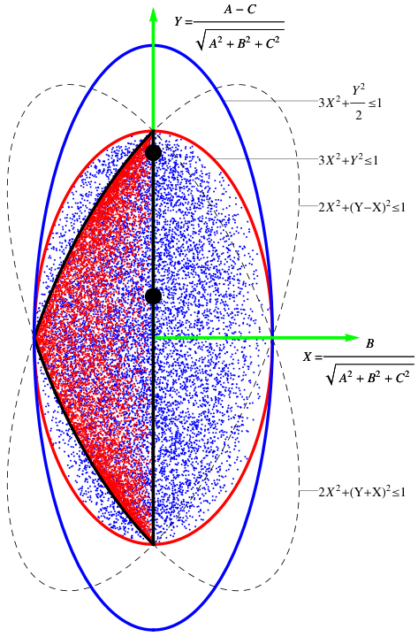
The Dirac bound is marked by the red ellipse; the analytic expression (derived in the appendix) to describe it is

The Majorana bound consists of parts of the two black dashed ellipses and a central vertical line, described by the expressions (also derived in the appendix)

The region bounded by the black solid line fulfills those three criteria. Besides, we also show Rosen’s Dirac bound ($0\leq R_{\rho}\leq 4$) by the blue ellipse, which in this formulation is $3X^{2}+Y^{2}/2\leq 1$. For Rosen’s Majorana bound, only the left half of the blue ellipse is allowed, i.e. $\sqrt{1/3-Y^{2}/6}\leq X\leq 0$. The two black dots on the central vertical line represent the SM values, without or with the CC interaction included, according to Eqs. (14) and (15), respectively.

So far we have only considered the case with neutrino energies much higher than charged lepton masses ($E_{\nu}\gg M$) so that all particles are assumed approximately massless. For low energy neutrino scattering, this approximation may not hold so we need to take the mass into account. For example, in reactor neutrino experiments, neutrino energies are typically at the MeV scale³³ 3 A typical reactor neutrino flux peaks roughly near 1 MeV and then decreases quickly above 2 MeV. However, the uncertainty of the flux below 2 MeV is quite large [36, 37]; often the events are selected from 3 MeV to 8 MeV. which are not much higher than the electron mass, 0.511 MeV. In this section, we consider the more general case with the charged lepton masses taken into account.

The result for the cross section of elastic scattering of neutrinos with massive charged leptons is

where

Note that the $A$, $B$, $C$ terms remain the same as the relativistic case [cf. Eqs. (9)-(13)] while the $D$ term is the only additional term that contains the contribution of nonzero charged lepton mass. It is the same for both the neutrino and antineutrino channels. In the SM, the value of $D$ is given by⁴⁴ 4 Note that in the relativistic case, $D$ is not measurable but it does not mean $D$ is zero. So for all the equations or conclusions in this section, to get their relativistic limit one needs to set $M\rightarrow 0$, not $D\rightarrow 0$.

From Eqs. (23) and (24) one can deduce that there are four parameters $(A,\thinspace B,\thinspace C,\thinspace D)$ that could be measured in non-relativistic neutrino scattering. If there were measurements of $(A,\thinspace B,\thinspace C,\thinspace D)$, then again their values could be used to distinguish between Dirac and Majorana neutrinos. The difference between the relativistic and non-relativistic cases is that in the former we have only three measurable quantities $(A,\thinspace B,\thinspace C)$ while in the latter we have four, $(A,\thinspace B,\thinspace C,\thinspace D)$. However, in both cases $(A,\thinspace B,\thinspace C)$ are subject to the same constraint shown in Fig. 1, which implies our previous bounds on $(A,\thinspace B,\thinspace C)$ in relativistic scattering also apply here. Actually if the scattering is quasi-relativistic, e.g. for reactor neutrinos scattering on electrons, $M/E_{\nu}$ is small⁵⁵ 5 But not negligibly small so that one still has to use Eqs. (23) or (24) instead of Eqs. (9) or (10)., and the measurement of $D$ would be the most inaccurate among the four quantities. So for such experiments, the most important quantities would still be $(A,\thinspace B,\thinspace C)$. In case $D$ were known, a ratio such as

could be studied. For Dirac neutrinos $R_{\sigma}$ lies within $[-4,4]$, while for Majorana neutrinos between $[-4,3]$.

Next, we shall study the Dirac and Majorana bounds in the presence of four measurable quantities $(A,\thinspace B,\thinspace C,\thinspace D)$. Similar to the relativistic case, the normalization of $(A,\thinspace B,\thinspace C,\thinspace D)$ is not important so we only care about their ratios. From the four quantities, we can define at most three independent ratios, we choose here

Note that $D^{2}$ appears in the denominator of the definition of $Z$, but not in $X$ and $Y$. In principle we could also put $D^{2}$ in the definitions of $X$ and $Y$, but we choose the current form because we want to keep the same definitions of $X$ and $Y$ as the relativistic case. As we have just mentioned, the previous bounds in the relativistic case on $(A,\thinspace B,\thinspace C)$ can also be used in the non-relativistic case and might probably be the most important bounds if the scattering is quasi-relativistic, so we prefer to define the first two ratios independent of $D$, which enable us to apply the relativistic bounds directly to the non-relativistic case.

With the three ratios, the problem essentially becomes finding the allowed regions in the $X$-$Y$-$Z$ space for Dirac and Majorana neutrinos. Finding the boundaries analytically as for the relativistic case in the previous section turns out to be much more complicated and difficult than the 2-dimensional problem that lead to Fig. 2. Though the projections of these regions in some special directions can be analytically computed, they can not provide a full description of the allowed regions. So instead, we will use a numerical method to find the allowed regions. We generate $10^{6}$ samples with random values of $(C_{a},\thinspace D_{a})$ in $[-1,1]$ and then compute the corresponding $(X,\thinspace Y,\thinspace Z)$ according to Eqs. (11)-(13), (25) and (28). Since the allowed regions are 3-dimensional objects, we display their 2-dimensional projection with various $Z$ values. The results are presented in Fig. , where blue points are for Dirac neutrinos and red for Majorana. For each fixed value of $Z$, the section shows the allowed values of $(X,\thinspace Y)$. As one may expect, combining the results of all possible $Z$ values should lead to a result analogous to that shown in Fig. 2.

As we have derived different bounds for Dirac and Majorana neutrinos in the presence of general interactions, we would like to confront these bounds with current experimental constraints. Possible experimental constraints may directly come from elastic neutrino scattering experiments such as CHARM [38], CHARM-II [39, 40], LAMPF [41], MINER$\nu$A [42], LSND [43] and TEXONO [44], or from other experiments sensitive to new neutrino interactions, such as LEP or observations of atmospheric, reactor, solar, and accelerator neutrinos in neutrino oscillation experiments.

A complete analysis including all possible experimental constraints is beyond the scope of this paper. Instead we will only focus on the strongest constraints from elastic neutrino scattering experiments⁶⁶ 6 Note that for the widely-studied Non-Standard Interaction (NSI) there has been a comprehensive study on the various constraints from present and future experiments [45]. It turns out that for $\varepsilon_{\mu\mu}^{e}$ and $\varepsilon_{ee}^{e}$, the current strongest constraints are from elastic neutrino scattering experiments (see table 2 in [45]). Therefore we expect that the strongest constraints on more general new interactions may also come from such experiments. This is one of the reasons that we only focus on elastic neutrino scattering experiments in this work., which provide direct measurements on $A$, $B$, $C$ and $D$ (if the scattering is relativistic, then $D$ can not be measured) according to Eqs. (9) and (10) or  (23) and (24).

Since our discussion in this section may refer to different channels such as $\nu_{\mu}+e$ or $\bar{\nu}_{e}+e$, we would like to distinguish them by adding subscripts of the corresponding lepton flavors. If the flavors of the neutrino and charged lepton are $\alpha$ and $\beta$ respectively $(\alpha,\thinspace\beta=e,\thinspace\mu,\thinspace\tau)$ then the corresponding $(A,\thinspace B,\thinspace C,\thinspace D)$ is denoted by $(A_{\alpha\beta},\thinspace B_{\alpha\beta},\thinspace C_{\alpha\beta},\thinspace D_{\alpha\beta})$, and $(X,\thinspace Y)$ by $(X_{\alpha\beta},\thinspace Y_{\alpha\beta})$.

The most interesting and promising channel to achieve a high precision of measurement are $(\alpha,\thinspace\beta)=(\mu,\thinspace e)$ or $(e,\thinspace e)$. In this paper, we will not include all the elastic neutrino scattering experiments but only two representative experiments, CHARM-II (for the $\mu e$ channel) and TEXONO (for the $ee$ channel) as they may provide the strongest constraints⁷⁷ 7 Actually their measurements of $s_{W}^{2}$ may be a good indicator of the precision, $s_{W}^{2}=0.2324\pm 0.0083$ in CHARM-II [40], $0.249\pm 0.063$ in LAMPF [41], $0.248\pm 0.051$ in LSND [43] and $0.251\pm 0.031\pm 0.024$ in TEXONO [44]. From $s_{W}^{2}$ we can expect that CHARM-II and TEXONO provide the strongest constraints on new interactions in the corresponding channels..

The CHARM-II collaboration has measured both $\nu_{\mu}$ and $\overline{\nu}_{\mu}$ neutrinos scattering on electrons with a mean neutrino energy at 20 GeV (i.e. the scattering is highly relativistic). The unfolded differential cross sections from this measurement have been published in [39], from which it is quite straightforward to perform a $\chi^{2}$-fit to obtain the constraint on $(A_{\mu e},\thinspace B_{\mu e},\thinspace C_{\mu e})$, including both $\nu_{\mu}$ and $\overline{\nu}_{\mu}$ data. We consider the following $\chi^{2}$-function:

where $s_{i}$ and $\sigma_{s,i}$ represent the measured differential cross section of $\nu_{\mu}+e^{-}$ and its uncertainty respectively. The antineutrino part is also included in the $\chi^{2}$-fit. The data of $s_{i}$ and $\sigma_{s,i}$, taken from [39], is shown in Fig. 3.

For any given $(A_{\mu e},\thinspace B_{\mu e},\thinspace C_{\mu e})$ we can compute the corresponding $\chi^{2}$-value according to Eq. (29). However, to distinguish between Dirac and Majorana neutrinos, what actually concerns us is $(X_{\mu e},\thinspace Y_{\mu e})$. One can convert the $\chi^{2}$-fit on $(A_{\mu e},\thinspace B_{\mu e},\thinspace C_{\mu e})$ to the corresponding fit on $(X_{\mu e},\thinspace Y_{\mu e})$ according to Eq. (19) if the normalization factor $R_{\mu e}$ is known. In this work, for simplicity, we fix $R_{\mu e}$ at the SM value. The result is presented in the left panel of Fig. 4 where the 90% C.L. constraint is shown by the blue region. The black and red points represent the SM value and the best fit, respectively.

From the left panel of Fig. 4 we can see that large deviations of $(X_{\mu e},\thinspace Y_{\mu e})$ from the the SM value (the black point) are still allowed by the CHARM-II constraint (the blue region), which covers both the Dirac and Majorana regions. Both the best fit (the red point) and the SM value (black point) are well compatible with data, which can be directly understood from the red and black curves in Fig. 3.

Currently a large part of the blue region (including the best fit) locates in the $X_{\mu e}>0$ region, which can only be reached if neutrinos are Dirac. Though the constraint is too weak⁸⁸ 8 Here we have only used the data of unfolded differential cross sections of CHARM-II [39]. The constraint obtained in this way is weaker than the actual constraint from the original event spectrum, because the unfolding process would inevitably lead to a loss of information of the original spectrum. Since the original event spectrum is not accessible to us, we have to use the unfolded data instead. to show any preference for Dirac or Majorana neutrinos, it illustrates how future measurements might enable us to determine the nature of neutrinos: such data may prefer a region inaccessible to Majorana neutrinos.

The TEXONO experiment [44] has measured elastic $\overline{\nu}_{e}+e^{-}$ reactor neutrino scattering with a CsI(Tl) crystal detector. The scattering events are selected from 3 MeV to 8 MeV. In this experiment, the electron mass is not negligible and should be taken into account. So we shall use the non-relativistic formula (24). The event rates in each recoil energy bin can be estimated by

where $\Delta T$ is the bin width and $\Phi(E_{\nu})$ is the reactor neutrino flux. We use the following $\chi^{2}$-function to fit the parameters in the cross section,

where $N_{i}^{0}$ and $\sigma_{N,i}$ are the observed event rates and the corresponding uncertainties, respectively. We take $\Phi(E_{\nu})$, $N_{i}^{0}$ and $\sigma_{N,i}$ all from [44]. The result is presented in the right panel of Fig. 4 where to convert the $\chi^{2}$-fit on $(A_{ee},\thinspace B_{ee},\thinspace C_{ee},\thinspace D_{ee})$ to $(X_{ee},\thinspace Y_{ee})$ we have fixed the normalization factors $R_{ee}$ and $D_{ee}$ to their SM values.

As is shown in Fig. 4, the current constraint from TEXONO not only allows both the Dirac and Majorana cases, but also allows the parameters to be outside the Dirac bound. Actually the current best fit (the red point) is just on the borderline of this case. Indeed, the red curve in Fig. 5 which is generated with the parameters at this point, shows directly that it can fit the TEXONO data very well. If the scattering parameters turn out to lie outside the Dirac bound, then this would imply exotic new physics that can not be described by the most general Lorentz invariant interactions in Eq. (1).

From the fits it is straightforward to obtain the current limits on the fundamental parameters $C_{a}$ and $D_{a}$ in Eqs. (1) and (4). The result is shown in Fig. 6. The fit assumes Dirac neutrinos, for Majorana neutrinos the results look very similar. As one can see, small values of tensor interactions and small departures from the SM values are allowed. Scalar and pseudo-scalar interactions are weakly constrained. Recently Ref. [46] published constraints on tensor and scalar interactions from TEXONO data, which as we have checked is consistent with our result.

Since the current constraints from CHARM-II and TEXONO allow both the Dirac and Majorana cases, we would like to investigate whether future experiments with improved sensitivities could distinguish between them. This possibility will crucially depend on how far away the actual values of $(X,\thinspace Y)$ are from the SM values. For illustration, we choose two points which are still in the $90\%$ C.L. bounds of CHARM-II and TEXONO, but significantly deviate from the SM values. Then we assume that future experiments have improved sensitivities so that compared to CHARM-II or TEXONO, the uncertainties of measurement would be reduced by a factor of 3 or 4, respectively. In Fig. 7, we show the $90\%$ C.L. bounds of such hypothetical experiments (the blue regions). We can see that if the actual values (the yellow points) deviate from the SM values (the black points) significantly, then such experiments could exclude Majorana neutrinos at more than $90\%$ C.L.

If neutrinos have new interactions beyond the SM, then their Dirac/Majorana nature could have observable differences in neutrino scattering, which are not suppressed by neutrino masses. We have performed an exhaustive study on all possible criteria that could be used to distinguish between Dirac and Majorana neutrinos in this context.

We have computed the cross sections of elastic neutrino-fermion scattering in the presence of the most general interactions including scalar, pseudo-scalar, vector, axial-vector and tensor interactions. The result is given by Eqs. (9), (10) for the relativistic case and it implies that there are at most three independent scattering parameters $(A,\thinspace B,\thinspace C)$ that could be measured in this case. These parameters are subject to certain bounds which depend on the Dirac/Majorana nature of neutrinos, as shown in Fig. 1 or Fig. 2 in terms of two ratios $(X,\thinspace Y)$ defined from $(A,\thinspace B,\thinspace C)$. Therefore the Dirac and Majorana bounds in Fig. 1 or Fig. 2 [for analytic expressions, see Eqs. (21) and (22)] could be used to determine the nature of neutrinos. If the parameters measured in neutrino scattering experiments are out of the Majorana bound but inside the Dirac bound, then neutrinos are Dirac particles.

As for the non-relativistic case, we find there is only one additional term in the cross sections [cf. Eqs. (23), (24)]. This extends the three scattering parameters $(A,\thinspace B,\thinspace C)$ in the relativistic case to four parameters $(A,\thinspace B,\thinspace C,\thinspace D)$ and the two ratios $(X,\thinspace Y)$ to three, $(X,\thinspace Y,\thinspace Z)$, with their explicit expressions given by Eq. (25) and Eq. (28). The corresponding Dirac and Majorana bounds are numerically found and presented in Fig. . Note that the bounds found for the relativistic case, i.e. without $D$, also apply to the non-relativistic case.

Currently the constraints from two neutrino scattering experiments, CHARM-II and TEXONO, are well consistent with both Dirac and Majorana neutrinos as shown in Fig. 4. Nevertheless they are able to effectively constrain the ratios $(X,\thinspace Y)$. If in the future neutrino scattering experiments would achieve much higher precision, deviations from the SM might be observed, from which one might be able to determine the nature of neutrinos. So far we have not included measurements from other experiments, which if combined may give stronger constraints.

Our analysis shows that there is still room for exciting new physics in the neutrino sector, and searches for new neutrino interactions are surely of large interest, as they can contribute to the exciting question of whether neutrinos are Dirac or Majorana particles.

References

- [1] W. Rodejohann, Int. J. Mod. Phys. E20, 1833 (2011), arXiv:1106.1334 [hep-ph] .
- [2] T. P. Cheng and L.-F. Li, Phys. Rev. Lett. 45, 1908 (1980).
- [3] B. Kayser and R. E. Shrock, Phys. Lett. B112, 137 (1982).
- [4] R. E. Shrock, Phys. Lett. B112, 382 (1982a).
- [5] R. E. Shrock, Nucl. Phys. B206, 359 (1982b).
- [6] S. P. Rosen, Phys. Rev. Lett. 48, 842 (1982).
- [7] T. Garavaglia, Phys. Rev. D29, 387 (1984).
- [8] S. M. Barr and A. Halprin, Phys. Lett. B202, 279 (1988).
- [9] T. Chhabra and P. R. Babu, Phys. Rev. D46, 903 (1992).
- [10] V. B. Semikoz, Nucl. Phys. B498, 39 (1997), arXiv:hep-ph/9611383 [hep-ph] .
- [11] M. Zralek, Recent progress in theory and phenomenology of fundamental interactions. Proceedings, 21st School of Theoretical Physics, Ustron, Poland, September 19-24, 1997, Acta Phys. Polon. B28, 2225 (1997), arXiv:hep-ph/9711506 [hep-ph] .
- [12] I. V. Gaidaenko, Phys. Atom. Nucl. 61, 116 (1998), [Yad. Fiz.61,125(1998)].
- [13] D. Singh, N. Mobed, and G. Papini, Phys. Rev. Lett. 97, 041101 (2006), arXiv:gr-qc/0605153 [gr-qc] .
- [14] A. Menon and A. M. Thalapillil, Phys. Rev. D78, 113003 (2008), arXiv:0804.3833 [hep-ph] .
- [15] R. Szafron and M. Zralek, Acta Phys. Polon. B40, 3041 (2009).
- [16] C.-Y. Chen and P. S. B. Dev, Phys. Rev. D85, 093018 (2012), arXiv:1112.6419 [hep-ph] .
- [17] R. Szafron and M. Zralek, Phys. Lett. B718, 113 (2012), arXiv:1210.2996 [hep-ph] .
- [18] D. N. Dinh, S. T. Petcov, N. Sasao, M. Tanaka, and M. Yoshimura, Phys. Lett. B719, 154 (2013), arXiv:1209.4808 [hep-ph] .
- [19] S. A. Alavi and A. Abbasnezhad, Grav. Cosmol. 22, 288 (2016), arXiv:1201.4741 [hep-ph] .
- [20] Z.-z. Xing, Phys. Rev. D87, 053019 (2013), arXiv:1301.7654 [hep-ph] .
- [21] J. Barranco, D. Delepine, V. Gonzalez-Macias, C. Lujan-Peschard, and M. Napsuciale, Phys. Lett. B739, 343 (2014), arXiv:1408.3219 [hep-ph] .
- [22] J.-M. Frere, J. Heeck, and S. Mollet, Phys. Rev. D92, 053002 (2015), arXiv:1506.02964 [hep-ph] .
- [23] J. Gluza, T. Jelinski, and R. Szafron, Phys. Rev. D93, 113017 (2016), arXiv:1604.01388 [hep-ph] .
- [24] C. O. Dib, C. S. Kim, K. Wang, and J. Zhang, Phys. Rev. D94, 013005 (2016), arXiv:1605.01123 [hep-ph] .
- [25] C. S. Kim and D. Sahoo, (2016), arXiv:1612.00607 [hep-ph] .
- [26] W. Sobkow and A. Blaut, Eur. Phys. J. C76, 550 (2016), arXiv:1607.03536 [hep-ph] .
- [27] B. Kayser, Phys. Rev. D26, 1662 (1982).
- [28] M. Lindner, W. Rodejohann, and X.-J. Xu, (2016), arXiv:1612.04150 [hep-ph] .
- [29] G. V. Dass, Phys. Rev. D32, 1239 (1985).
- [30] S. Bergmann, Y. Grossman, and E. Nardi, Phys. Rev. D60, 093008 (1999), arXiv:hep-ph/9903517 [hep-ph] .
- [31] B. Kayser, E. Fischbach, S. P. Rosen, and H. Spivack, Phys. Rev. D20, 87 (1979).
- [32] R. L. Kingsley, F. Wilczek, and A. Zee, Phys. Rev. D10, 2216 (1974).
- [33] V. Shtabovenko, R. Mertig, and F. Orellana, Comput. Phys. Commun. 207, 432 (2016), arXiv:1601.01167 [hep-ph] .
- [34] R. Mertig, M. Bohm, and A. Denner, Comput. Phys. Commun. 64, 345 (1991).
- [35] H. H. Patel, Comput. Phys. Commun. 197, 276 (2015), arXiv:1503.01469 [hep-ph] .
- [36] V. I. Kopeikin, Phys. Atom. Nucl. 75, 143 (2012), [Yad. Fiz.75N2,165(2012)].
- [37] K. Schreckenbach, G. Colvin, W. Gelletly, and F. Von Feilitzsch, Phys. Lett. B160, 325 (1985).
- [38] J. Dorenbosch et al. (CHARM), Z. Phys. C41, 567 (1989), [Erratum: Z. Phys.C51,142(1991)].
- [39] P. Vilain et al. (CHARM-II), Phys. Lett. B302, 351 (1993).
- [40] P. Vilain et al. (CHARM-II), Phys. Lett. B335, 246 (1994).
- [41] R. C. Allen et al., Phys. Rev. D47, 11 (1993).
- [42] J. Park et al. (MINERvA), Phys. Rev. D93, 112007 (2016), arXiv:1512.07699 [physics.ins-det] .
- [43] L. B. Auerbach et al. (LSND), Phys. Rev. D63, 112001 (2001), arXiv:hep-ex/0101039 [hep-ex] .
- [44] M. Deniz et al. (TEXONO), Phys. Rev. D81, 072001 (2010), arXiv:0911.1597 [hep-ex] .
- [45] S. Davidson, C. Pena-Garay, N. Rius, and A. Santamaria, JHEP 03, 011 (2003), arXiv:hep-ph/0302093 [hep-ph] .
- [46] B. Sevda, M. Deniz, S. Kerman, L. Singh, H. T. Wong, and M. Zeyrek, (2016), arXiv:1611.07259 [hep-ex] .