Cache-Aided Content Delivery over Erasure Broadcast Channels

Wireless content caching is a promising technique to flatten the traffic over the backhaul network by shifting part of the traffic from peak to off-peak periods [1, 2, 3, 4, 5]. Video-on-demand services for mobile users would particularly benefit from content caching as a few highly popular files are requested by a large number of users over a relatively short time period. Popular contents that are likely to be requested by a majority of the users can be proactively cached at the network edge during a period of low network traffic, known as the placement phase. The delivery phase is performed during a peak traffic period, when the users reveal their demands, and the cached contents can be exploited to reduce both the load over the backhaul links and the latency in delivery [6].

A coded proactive content caching and delivery scheme has been proposed by Maddah-Ali and Niesen in [6, 7], where they consider a library of same-size files to be delivered over a noiseless broadcast channel (BC), while the receivers are equipped with cache memories of equal size. They identify a trade-off between the cache size and the minimum rate required during the delivery phase to serve all the receivers for all demand combinations, and show that coding can significantly reduce the required delivery rate. Several improved coded caching schemes and information theoretic performance bounds have been introduced since then [8, 9, 10, 11, 12, 13, 14, 15]. Coded caching has since been extended to various network settings, including device-to-device caching [16, 17], online cache placement [18], files with non-uniform popularities [19, 20] and distinct lengths [21], users with non-uniform cache sizes [22, 23], multi-layer caching [24], and caching by users with different distortion requirements [25, 26, 27].

In contrast to the setting introduced in [6], a noisy channel is considered for the delivery phase in [28, 29, 30, 31, 32, 33, 34, 35]. Here, we follow the model considered in [31], and assume that the delivery phase takes place over a memoryless packet erasure BC, which models a packetized communication system, where each packet is separately channel coded against errors at the physical layer, so that a packet either arrives at a receiver correctly, or is lost. Communication over Internet is usually modeled as a packet erasure channel. The receivers in the system are grouped into two disjoint sets of weak and strong receivers. All the weak receivers are assumed to have statistically worse channels than the strong receivers, while the users in each set can have arbitrary erasure probabilities. To compensate for the worse channel quality, each weak receiver is equipped with a cache memory of equal size. We consider the case when the number of receivers is not greater than the number of files in the library. Assuming equal-rate files in the library, we derive a trade-off between the size of the caches provided to the weak receivers and the rate of the files, for which any demand combination can be reliably satisfied over the erasure BC. The proposed scheme exploits a novel file subpacketization, and performs a different caching and content delivery scheme to deliver different subpackets over the channel. Moreover, the delivery of the contents to the weak and strong receivers are coupled through the use of a joint encoding scheme to maximally benefit from the available cache memories. We show that, when specified to the homogeneous scenario considered in [31], where the receivers in the same set have the same erasure probability, the proposed scheme outperforms the one in [31].

The rest of this paper is organized as follows. We introduce the system model in Section II. Main results are summarized and compared with the state-of-the-art in Section III. The proposed scheme is elaborated and analyzed in Section IV. We conclude the paper in Section V.

Notations: For two integers $i\leq j$, the set $\left\{i,i+1,...,j\right\}$ is denoted by $\left[i:j\right]$, and the set $[1:i]$ is shortly denoted by $[i]$. For two sets $\mathcal{Q}$ and $\mathcal{P}$, $\mathcal{Q}\backslash\mathcal{P}$ is the set of elements in $\mathcal{Q}$ that do not belong to $\mathcal{P}$. Notation $\left|\cdot\right|$ represents the cardinality of a set, or the length of a vector. Notation $\oplus$ refers to bitwise XOR operation; and finally, $\binom{j}{i}$ returns the binomial coefficient “$j$ choose $i$”.

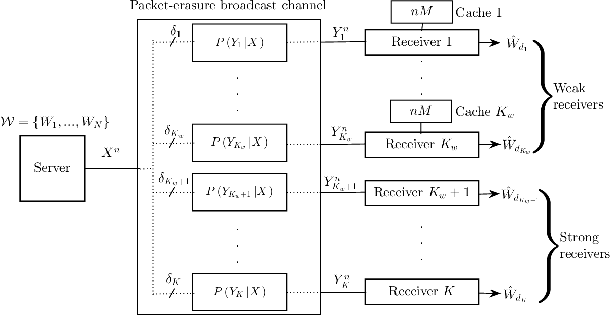
We consider a server with a library of $N$ popular files $\mathbf{W}\mathrel{\mathop{\kern 0.0pt=}\limits^{\Delta}}\left(W_{1},...,W_{N}\right)$. Each file $W_{f}$ is distributed uniformly over the set $\left[{\left\lceil{{2^{nR}}}\right\rceil}\right]$, $\forall f\in\left[N\right]$, where $R$ denotes the rate of each file, and $n$ is the number of channel uses during the delivery phase. Receiver $k$’s demand is represented by $d_{k}$, where $d_{k}\in\left[N\right]$, $\forall k\in\left[K\right]$. The server delivers all the requests $W_{d_{1}},...,W_{d_{K}}$ to their corresponding receivers simultaneously over a BC.

Following [31], the channel between the server and the receivers is modeled as a memoryless packet erasure BC. For each channel use, the server transmits an $F$-bit codeword from the alphabet $\mathcal{X}\mathrel{\mathop{\kern 0.0pt=}\limits^{\Delta}}\left\{0,1\right\}^{F}$, and the output alphabet at each receiver is $\mathcal{Y}\mathrel{\mathop{\kern 0.0pt=}\limits^{\Delta}}\mathcal{X}\cup\left\{\Delta\right\}$, where the erasure symbol $\Delta$ corresponds to a packet that is not received at the receiver. Receiver $k$, for $k\in\left[K\right]$, receives the transmitted codeword $x\in\mathcal{X}$ correctly with probability $1-\delta_{k}$, and the erasure symbol $\Delta$ with probability $\delta_{k}$. Thus, given the transmitted codeword $x\in\mathcal{X}$, receiver $k\in[K]$ observes the output $y_{k}\in\mathcal{Y}$ with the conditional probability

Two disjoint sets of receivers, weak and strong receivers, are considered, grouped according to the erasure probabilities of their channels. These groups may model users located in areas with relatively bad and good network coverage, respectively. We assume that the channel condition of each strong receiver is statistically better than that of each weak receiver; that is, the erasure probability of a strong receiver is lower than any weak receiver. Without loss of generality, we enumerate the receivers in the order of improving channel quality, that is, we have $\delta_{1}\geq\delta_{2}\geq\cdots\geq\delta_{K}$. We denote the set of erasure probabilities by $\boldsymbol{\delta}\mathrel{\mathop{\kern 0.0pt=}\limits^{\Delta}}\left\{\delta_{1},\delta_{2},...,\delta_{K}\right\}$. We denote the first $K_{w}$ receivers as the weak receivers, and the next $K_{s}=K-K_{w}$ receivers as the strong receivers. To compensate for their poorer channel quality, each weak receiver is equipped with a cache memory of size $nM$ bits, as depicted in Fig. 1. The special case in which all the receivers in the same set have the same erasure probability; that is, all the weak receivers have erasure probability $\delta_{w}$, and all the strong receivers have erasure probability $\delta_{s}$, with $\delta_{s}<\delta_{w}$, is called the homogeneous scenario. The set of erasure probabilities for the homogeneous scenario is represented by ${\boldsymbol{\delta}}_{ws}$.

Content delivery is performed in two phases [6]. It starts with the placement phase which takes place during the off-peak traffic period, and the caches of the weak receivers are filled without the knowledge of their future demands. Thus, only the weak receivers take part in the placement phase, and the contents of the cache of receiver $k$, for $k\in\left[K_{w}\right]$, at the end of this phase is denoted by $Z_{k}$. Note that, $Z_{k}$ does not depend on any specific demand combination, and it is instead a function of the library $\mathbf{W}$. The caching function for receiver $k\in\left[K_{w}\right]$ is given by

which maps the entire library to the cache content $Z_{k}$, i.e., $Z_{k}={\phi_{k}}\left(\mathbf{W}\right)$. It is to be noted that, since the placement phase is performed over a low-congestion period, it is assumed that no erasure occurs during this phase.

The delivery phase follows once the demands of the receivers are revealed to the server, which transmits a length-$n$ codeword $X^{n}$ over the erasure BC. For a demand vector $\mathbf{d}\mathrel{\mathop{\kern 0.0pt=}\limits^{\Delta}}(d_{1},...,d_{K})$, a coded delivery function

generates a common message $X^{n}$ as a function of the entire library and the receiver demands, i.e., $X^{n}=\psi\left(\mathbf{W},\mathbf{d}\right)$, to be delivered over the erasure BC. Each receiver $k\in\left[K\right]$ observes $Y_{k}^{n}$ according to (1). Each weak receiver $k\in\left[K_{w}\right]$ tries to decode $W_{d_{k}}$ from its channel output $Y_{k}^{n}$ along with the content available locally in its cache and the demand vector d, utilizing the decoding function

i.e., the reconstructed file by each weak receiver $k\in\left[K_{w}\right]$ is

On the other hand, to serve the users with demand vector d, each strong receiver $k\in\left[K_{w}+1:K\right]$ reconstructs its demand $W_{d_{k}}$ solely from its channel output $Y_{k}^{n}$ through the decoding function

which generates the reconstructed file

We would like to note that the capacity of the above caching network remains an open problem even when the delivery channel is an error-free shared bit pipe except for the network with an uncoded cache placement phase [11]. Here, our goal is to identify achievable memory-rate pairs that improve upon the state-of-the-art.

Following well-known results from multi-user information theory are included here for completeness as they will be instrumental in deriving our results later in the paper.

Next, we consider the packet erasure BC with side information, and provide an achievable rate pair based on the joint encoding scheme of [37]. Here we briefly overview the coding scheme and the proof of achievability, and refer the reader to [37] for details. Consider two receivers with erasure probabilities $\delta_{1}\geq\delta_{2}$. Let $W_{1}$ and $W_{2}$, distributed uniformly over $\left[2^{nR_{1}}\right]$ and $\left[2^{nR_{2}}\right]$, denote the messages targeted for receivers 1 and 2, respectively. We assume that message $W_{2}$ is available as side information at receiver 1, the weak receiver. We present a coding scheme and the corresponding achievable rate region based on the joint encoding scheme of [37]. For a fixed distribution $P\left(X\right)$, we generate $2^{n\left(R_{1}+R_{2}\right)}$ codewords of length $n$, $x^{n}\left(w_{1},w_{2}\right)$, $w_{1}\in\left[2^{nR_{1}}\right]$, $w_{2}\in\left[2^{nR_{2}}\right]$, where each entry of each codeword is generated independently according to $P\left(X\right)$. The codebook is revealed to the transmitter and the receivers. To transmit particular messages $W_{1}=w_{1}$ and $W_{2}=w_{2}$, the codeword $x^{n}\left(w_{1},w_{2}\right)$ is transmitted over the BC. In the proposed coding scheme, the good receiver, i.e., receiver 2, decodes both messages; and therefore, it tries to find a unique pair $\left({\hat{w}}_{1},{\hat{w}}_{2}\right)\in\left[2^{nR_{1}}\right]\times\left[2^{nR_{2}}\right]$, such that $\left(X^{n}\left({\hat{w}}_{1},{\hat{w}}_{2}\right),y_{2}^{n}\right)$ belongs to the jointly typical set defined in [38]. The probability of decoding error tends to $0$ as $n$ goes to infinity, if

The first receiver already knows $W_{2}$ as side information; therefore, it only needs to decode $W_{1}$; thus, it looks for a unique index ${\hat{w}}_{1}\in\left[2^{nR_{1}}\right]$ such that $\left(X^{n}\left({\hat{w}}_{1},{W}_{2}\right),y_{1}^{n}\right)$ belongs to the typical set [38]. The probability of error tends to $0$ as $n$ goes to infinity, if

For the packet erasure BC, both mutual information terms are maximized with a uniform input, and the following conditions are obtained:

We can easily generalize this coding scheme to multiple receivers and obtain the achievable rate region stated in the following proposition (also provided in [31]).

For notational convenience, in the rest of the paper we use

to represent the transmission of message $W_{1}$ to the receivers in set $\mathcal{S}_{1}$, and message $W_{2}$ to the receivers in set $\mathcal{S}_{2}$ using the outlined joint encoding scheme, where ${\mathcal{S}_{1}}\cap{\mathcal{S}_{2}}=\emptyset$, and $W_{2}$ is available at all the receivers in $\mathcal{S}_{1}$ as side information.

A coding scheme as well as an information theoretic upper bound on the capacity of the above caching and delivery network are proposed in [31] for the homogeneous scenario. Here, we present a new coding scheme, called the successive cache-channel coding (SCC) scheme, for delivery over any packet erasure BC, which is shown to improve upon the one in [31] in the homogeneous scenario. We present the $(M,R)$ pairs achieved by this scheme in Theorem 1 below. The details of the scheme are presented in Section IV.

Next, we compare the achievable rate of the SCC scheme for the homogeneous scenario with the scheme of [31], which we will refer to as the STW scheme. In Fig. 2, the achievable memory-rate trade-off of the SCC scheme is compared with the STW scheme when $K_{w}=2$, $K_{s}=2$, $N=20$, $F=10$, $\delta_{s}=0.2$, and $\delta_{w}=0.8$. The upper bound on the capacity of the cache-aided packet erasure BC derived in [31, Theorem 7] is also included. The SCC scheme outperforms the STW scheme due to the improved achievable memory-rate pair $\left(M_{(0,2)},R_{(0,2)}\right)$, which is not achievable by the STW scheme. This improvement can be extended to a wider range of cache sizes through memory-sharing, also reducing the gap to the upper bound.

In Fig. 3, we plot the achievable rates for both schemes in the homogeneous scenario with $K_{w}=7$, $K_{s}=10$, $N=50$, $F=20$, $\delta_{s}=0.2$, and $\delta_{w}=0.9$. The upper bound on the capacity derived in [31, Theorem 7] is also included. Observe that, for relatively small cache sizes, where the best memory-rate trade-off is achieved by time-sharing between $\left(M_{(0,0)},R_{(0,0)}\right)$ and $\left(M_{(0,1)},R_{(0,1)}\right)$, and for relatively large cache sizes, where the best memory-rate trade-off is achieved by time-sharing between $\left(M_{(6,7)},R_{(6,7)}\right)$ and $\left(M_{(7,7)},R_{(7,7)}\right)$, both schemes achieve the same rate; however, the proposed SCC scheme achieves a higher rate than STW scheme for all other intermediate cache sizes, and reduces the gap to the upper bound. For a cache capacity of $M=30$, the SCC scheme provides approximately $15\%$ increase in the achievable rate compared to the STW scheme.

In Fig. 4, the achievable rates of the SCC and STW schemes in the homogeneous scenario are compared for different values of $\delta_{w}$. System parameters considered in this comparison are $K_{w}=20$, $K_{s}=10$, $N=100$, $F=50$, $\delta_{s}=0.2$, and $\delta_{w}=0.7,0.8,0.9$. Observe that, unlike the STW scheme, the performance of the SCC scheme does not deteriorate notably for intermediate and relatively high cache capacities when $\delta_{w}$ increases, i.e., having worse channel qualities for the weak receivers. This is because the SCC scheme successfully exploits the available cache capacities, and there is little to lose from increasing $\delta_{w}$ when $M$ is sufficiantly large. Moreover, the superiority of the SCC scheme over the STW scheme is more pronounced for higher values of $\delta_{w}$, in which case, exploiting the cache memories available at the weak receivers more effectively through SCC becomes more important.

For the heterogeneous scenario, the capacity of the network under consideration is upper bounded by [31]

In Fig. 5, the effect of $K_{w}$ is considered for the heterogeneous scenario with the system parameters $K=15$, $N=100$, $F=10$, $\delta_{k}=0.9-0.01k$, for $k=1,...,5$, and $\delta_{l}=0.2-0.01l$, for $l=6,...,15$. In this figure, the achievable rates are plotted with respect to the total cache capacity of $K_{w}M$ for four different values for the number of weak receivers in the system, $K_{w}=4,5,10,15$. Note that the erasure probabilities are set such that the first $5$ receivers have significantly worse channels than the remaining $10$ receivers. Note also that the parameter $K_{w}$ determines which receivers are provided with cache memories. As it can be seen, the setting with $K_{w}=5$ achieves significantly higher rates over a wide range of total cache capacities compared to the other settings under consideration. If receiver $5$, which has a relatively bad channel quality, is not provided with any cache memory, and only the first 4 receivers are equipped with cache memories, i.e., $K_{w}=4$, the performance degrades significantly except for very small values of total cache size. This is because the first five receivers have much worse channel qualities, and the performance depends critically on the caches provided to all these five weak receivers. On the other hand, equipping receivers with relatively good channel qualities with cache memories deteriorates the performance of the system in terms of the achievable rate. Note that this is because the total available cache capacity is allocated across a larger number of receivers. This result confirms that it is more beneficial to allocate cache memories to the receivers with relatively worse channel qualities. The upper bound on the achievable rate for the setting with $K_{w}=5$ and $K_{s}=10$ is also included in this figure. We observe that the gap between the upper bound and the achievable rate for the same setting is relatively small for a wide range of cache sizes.

Before presenting the SCC scheme for the general heterogeneous scenario, in which we allow the weak and strong receivers to have distinct erasure probabilities, the main ideas behind this scheme are illustrated on an example in the simplified homogeneous scenario.

For notational convenience, the $i$-element subsets of set $[K_{w}]$ are enumerated by $\mathcal{S}_{1}^{(i)},\mathcal{S}_{2}^{(i)},...,$ $\mathcal{S}_{\binom{K_{w}}{i}}^{(i)}$, i.e.,

Next, we present the SCC scheme for a general heterogeneous scenario, achieving the memory-rate pair $\left(M_{(p,q)},R_{(p,q)}\right)$ given by (19), for any $p\in\left[0:K_{w}\right]$ and $q\in\left[p:K_{w}\right]$. For a given $(p,q)$ pair, where $p\in\left[0:K_{w}\right]$ and $q\in\left[p:K_{w}\right]$, each file $W_{f}$, $f\in[N]$, is divided into $(q-p+1)$ non-overlapping subfiles, represented by

References

- [1] L. W. Dowdy and D. V. Foster, “Comparative models of the file assignment problem,” ACM Comput. Surv., vol. 14, pp. 287–313, Jun. 1982.
- [2] K. C. Almeroth and M. H. Ammar, “The use of multicast delivery to provide a scalable and interactive video-on-demand service,” IEEE J. Sel. Areas Commun., vol. 14, no. 6, pp. 1110–1122, Aug. 1996.
- [3] A. Meyerson, K. Munagala, and S. Plotkin, “Web caching using access statistics,” in Proc. ACM-SIAM SODA, Washington, D.C., USA, Jan. 2001, pp. 354–363.
- [4] I. Baev, R. Rajaraman, and C. Swamy, “Approximation algorithms for data placement problems,” SIAM J. Comput., vol. 38, no. 4, pp. 1411–1429, Jul. 2008.
- [5] S. Borst, V. Gupta, and A. Walid, “Distributed caching algorithms for content distribution networks,” in Proc. IEEE INFOCOM, San Diego, CA, Mar. 2010, pp. 1–9.
- [6] M. A. Maddah-Ali and U. Niesen, “Fundamental limits of caching,” IEEE Trans. Inform. Theory, vol. 60, no. 5, pp. 2856–2867, May 2014.
- [7] ——, “Decentralized caching attains order optimal memory-rate tradeoff,” IEEE/ACM Trans. Netw., vol. 23, no. 4, pp. 1029–1040, Apr. 2014.
- [8] Z. Chen, P. Fan, and K. B. Letaief, “Fundamental limits of caching: Improved bounds for users with small buffers,” IET Communications, vol. 10, no. 17, pp. 2315–2318, Nov. 2016.
- [9] M. Mohammadi Amiri and D. Gündüz, “Fundamental limits of coded caching: Improved delivery rate-cache capacity trade-off,” IEEE Trans. Commun., vol. 65, no. 2, pp. 806–815, Feb. 2017.
- [10] M. Mohammadi Amiri, Q. Yang, and D. Gündüz, “Coded caching for a large number of users,” in Proc. Information Theory Workshop (ITW), Cambridge, UK, Sep. 2016, pp. 171–175.
- [11] Q. Yu, M. A. Maddah-Ali, and A. S. Avestimehr, “The exact rate-memory tradeoff for caching with uncoded prefetching,” arXiv:1609.07817v1 [cs.IT], Sep. 2016.
- [12] C. Tian, “Symmetry, outer bounds, and code constructions: A computer-aided investigation on the fundamental limits of caching,” arXiv:1611.00024v1 [cs.IT], Oct. 2016.
- [13] A. Sengupta, R. Tandon, and T. C. Clancy, “Improved approximation of storage-rate tradeoff for caching via new outer bounds,” in Proc. IEEE Int’l Symp. on Inform. Theory (ISIT), Hong Kong, Jun. 2015, pp. 1691–1695.
- [14] H. Ghasemi and A. Ramamoorthy, “Improved lower bounds for coded caching,” in Proc. IEEE Int’l Symp. on Inform. Theory (ISIT), Hong Kong, Jun. 2015, pp. 1696–1700.
- [15] C.-Y. Wang, S. H. Lim, and M. Gastpar, “A new converse bound for coded caching,” in Proc. Information Theory and Applications Workshop (ITA), La Jolla, CA, Jan.-Feb. 2016, pp. 1–6.
- [16] M. Gregori, J. Gomez-Vilardebo, J. Matamoros, and D. Gündüz, “Wireless content caching for small cell and D2D networks,” IEEE J. Sel. Areas Commun., vol. 34, no. 5, pp. 1222–1234, May 2016.
- [17] M. Ji, G. Caire, and A. F. Molisch, “Fundamental limits of caching in wireless D2D networks,” IEEE Trans. Inform. Theory, vol. 62, no. 2, pp. 849–869, Dec. 2015.
- [18] R. Pedarsani, M. A. Maddah-Ali, and U. Niesen, “Online coded caching,” in Proc. IEEE Int’l Conf. Commun. (ICC), Sydney, Australia, Jun. 2014, pp. 1878–1883.
- [19] U. Niesen and M. A. Maddah-Ali, “Coded caching with nonuniform demands,” in Proc. IEEE Conf. Comput. Commun. Workshops (INFOCOM WKSHPS), Toronto, ON, Apr. 2014, pp. 221–226.
- [20] J. Zhang, X. Lin, and X. Wang, “Coded caching under arbitrary popularity distributions,” in Proc. Infor. Theory Applications Workshop (ITA), San Diego, CA, Feb. 2015, pp. 98–107.
- [21] J. Zhang, X. Lin, C. C. Wang, and X. Wang, “Coded caching for files with distinct file sizes,” in Proc. IEEE Int’l Symp. on Inform. Theory (ISIT), Hong Kong, Jun. 2015, pp. 1686–1690.
- [22] S. Wang, W. Li, X. Tian, and H. Liu, “Coded caching with heterogenous cache sizes,” arXiv:1504.01123v3 [cs.IT], Apr. 2015.
- [23] M. Mohammadi Amiri, Q. Yang, and D. Gündüz, “Decentralized coded caching with distinct cache capacities,” arXiv:1601.05690v1 [cs.IT], Nov. 2016.
- [24] N. Karamchandani, U. Niesen, M. A. Maddah-Ali, and S. Diggavi, “Hierarchical coded caching,” in Proc. IEEE Int’l Symp. on Inform. Theory (ISIT), Honolulu, HI, Jun. 2014, pp. 2142–2146.
- [25] Q. Yang and D. Gündüz, “Centralized coded caching for heterogeneous lossy requests,” arXiv:1604.08178v1 [cs.IT], Apr. 2016.
- [26] P. Hassanzadeh, E. Erkip, J. Llorca, and A. Tulino, “Distortion-memory tradeoffs in cache-aided wireless video delivery,” arXiv:1511.03932v1 [cs.IT], Nov. 2015.
- [27] R. Timo, S. B. Bidokhti, M. Wigger, and B. Geiger, “A rate-distortion approach to caching,” in Proc. International Zurich Seminar on Communications, Zurich, Switzerland, Mar. 2016.
- [28] J. Zhang and P. Elia, “Fundamental limits of cache-aided wireless BC: Interplay of coded-caching and CSIT feedback,” IEEE Trans. Inform. Theory, vol. 63, no. 5, pp. 3142–3160, May 2017.
- [29] A. Ghorbel, M. Kobayashi, and S. Yang, “Content delivery in erasure broadcast channels with cache and feedback,” IEEE Trans. Inform. Theory, vol. 62, no. 11, pp. 6407–6422, Nov. 2016.
- [30] R. Timo and M. Wigger, “Joint cache-channel coding over erasure broadcast channels,” in Proc. IEEE Int’l Symp. on Wirel. Commun. Systems (ISWCS), Brussels, Belgium, Aug. 2015, pp. 201–205.
- [31] S. Saeedi Bidokhti, R. Timo, and M. Wigger, “Noisy broadcast networks with receiver caching,” arXiv:1605.02317v1 [cs.IT], May 2016.
- [32] W. Huang, S. Wang, L. Ding, F. Yang, and W. Zhang, “The performance analysis of coded cache in wireless fading channel,” arXiv:1504.01452v1 [cs.IT], Apr. 2015.
- [33] M. Maddah-Ali and U. Niesen, “Cache-aided interference channels,” arXiv: 1510.06121v1 [cs.IT], Oct. 2015.
- [34] N. Naderializadeh, M. Maddah-Ali, and A. S. Avestimehr, “Fundamental limits of cache-aided interference management,” arXiv:1602.04207v1 [cs.IT], Feb. 2016.
- [35] J. Zhang and P. Elia, “Wireless coded caching: A topological perspective,” arXiv:1606.08253v1 [cs.IT], Jun. 2016.
- [36] R. L. Urbanke and A. D. Wyner, “Packetizing for the erasure broadcast channel with an internet application,” in Proc. Int’l. Conf. Combinatorics, Information Theory and Statistics, Portland, ME, May 1997, p. 93.
- [37] E. Tuncel, “Slepian-Wolf coding over broadcast channels,” IEEE Trans. Inform. Theory, vol. 52, no. 4, pp. 1469–1482, Apr. 2006.
- [38] A. El Gamal and Y.-H. Kim, Network information theory. Cambridge, UK: Cambridge University Press, 2012.