Completing a joint PMF from projections: a low-rank coupled tensor factorization approach

Consider the setting where we are given a partially observed dataset of $M$ discrete samples $\left(x_{1}^{(i)},x_{2}^{(i)},\ldots,x_{N}^{(i)}\right)$, $i=1,\ldots,M,$ and we are interested in predicting the missing entries. This scenario often arises in recommender systems where we are interested in predicting user preferences, pertaining to news, movies or music, based on a user’s history as well as the history of other users.

Among the various approaches used in recommender systems, data completion using matrix and (more recently) tensor factorization is one of the most pervasive. The premise of factorization-based recommendation approaches is that the data approximately follow a low-rank model, i.e., there are few basic types of customers (and movies, songs, or news items), and every customer (movie, song, story) is a linear combination of the respective types. Thus a low-rank model is appropriate for the data, and can be used for completion.

In this paper, we propose a fundamentally different approach. From a statistical inference point of view, having access to the joint distribution of all variables of interest is the ‘gold standard’. Given the joint Probability Mass Function (PMF) of a set of discrete random variables, it is possible to compute any marginal or conditional probability for subsets of these variables, and use it to solve regression or classification problems. For example, one may be interested in finding the Maximum A Posteriori (MAP) estimate of an unobserved entry, or its conditional expectation given a number of observed variables. In practice however, it is often not possible to learn a joint PMF of all random variables without making restrictive assumptions, due to computational or statistical reasons; the number of free parameters grows exponentially in the number of variables. In addition, when the dataset is incomplete an imputation mechanism is needed.

In this work, we propose modeling a joint PMF of a set of random variables using a low-rank non-negative tensor (multi-way array) factorization model. In effect, we propose using a low-rank model of the joint PMF, as opposed to using a low-rank model of the raw data. Tensor factorization techniques are widely used in numerous diverse fields such as signal processing, computer vision, chemistry and more recently in machine learning and data mining [1]. Canonical Polyadic Decomposition (CPD) also known as PARAllel FACtor analysis (PARAFAC) [2, 3] and the Tucker decomposition [4] are the two most widely used factorization models. In this work, we focus on the CPD model which is known to be unique under mild conditions.

Any joint PMF of size $I_{1}\times\cdots\times I_{N}$ can be regarded as a non-negative CPD model of non-negative rank $\leq\underset{k}{\min}(\prod_{\begin{subarray}{c}n=1\\ n\neq k\end{subarray}}^{N}I_{n})$ – this is easy to see, using the same argument as for real-valued CPD in [1], and the trivial factorization ${\bf A}={\bf A}{\bf I}$. Symmetric CPD has been considered for the related (but different) problem of modeling co-occurrence data [5, 6]. The most relevant prior work is [7] (and [8]), where CPD (resp. Tucker) was used to model the joint PMF of multivariate categorical data, assuming access to the full joint PMF.

We do not assume access to the full joint PMF. The reason is that, when dealing with many random variables (large $N$), the probability of encountering any particular realization decays very fast (usually exponentially) as a function of $N$. That makes joint PMF estimation, even from complete samples, essentially intractable. One needs very long data records (very high $M$) for reliable estimates of the joint PMF values. In this paper, we show how we can utilize information regarding lower-order marginals of subsets of the random variables to provably infer the full joint PMF. Estimates of lower-order marginals are easier to compute even in the case of missing data, and a low-rank CPD model has the advantage of reducing the dimension of the parameter space, which becomes linear in the number of variables. We formulate the problem as a coupled tensor factorization problem and derive an algorithmic approach to solve it. We illustrate the method using synthetic data and give a motivating example using real data for rating prediction.

$N$-way tensor $\underline{\mathbf{X}}\in\mathbb{R}^{I_{1}\times I_{2}\times\cdots\times I_{N}}$ admits a CPD of rank $F$ if it can be decomposed as a sum of $F$ rank-1 tensors

$$\underline{\mathbf{X}}=\sum_{f=1}^{F}\boldsymbol{\lambda}(f)\mathbf{A}_{1}(:,f)\circ\mathbf{A}_{2}(:,f)\circ\cdots\circ\mathbf{A}_{N}(:,f),$$

(1)

where $\boldsymbol{\lambda}\in\mathbb{R}^{F},\mathbf{A}_{n}\in\mathbb{R}^{I_{n}\times F},n=1,2,\ldots,N$ and $F$ is the smallest number for which such a decomposition exists (Fig. 1). We then write $\underline{\mathbf{X}}=[\![\boldsymbol{\lambda},\mathbf{A}_{1},\ldots,\mathbf{A}_{N}]\!]$, with elements

$$\underline{\mathbf{X}}(i_{1},\ldots,i_{N})=\\ \sum_{f=1}^{F}\boldsymbol{\lambda}(f)\mathbf{A}_{1}(i_{1},f)\mathbf{A}_{2}(i_{2},f)\cdots\mathbf{A}_{N}(i_{N},f).$$

(2)

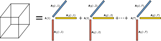
We denote the mode-$n$ matrix unfolding of $\underline{\mathbf{X}}$ as the matrix ${\mathbf{X}}^{(n)}$ of size $\prod_{\begin{subarray}{c}k=1\\ k\neq n\end{subarray}}^{N}I_{k}\times I_{n}$. We have that $\underline{\mathbf{X}}(i_{1},i_{2},\ldots,i_{N})={\mathbf{X}}^{(n)}(j,i_{n})$, where

$$j=1+\sum_{\begin{subarray}{c}k=1\\ k\neq n\end{subarray}}^{N}(i_{k}-1)J_{k}\;\text{with}\;J_{k}=\prod_{\begin{subarray}{c}m=1\\ m\neq n\end{subarray}}^{k-1}I_{m}.$$

(3)

The mode-$n$ matrix unfolding can be expressed as

$${\mathbf{X}}^{(n)}=\left(\underset{j\neq n}{\underset{j=1}{\overset{N}{\odot}}}\mathbf{A}_{j}\right)\mathcal{D}(\boldsymbol{\lambda})\mathbf{A}_{n}^{T},$$

(4)

where

$$\underset{j\neq n}{\underset{j=1}{\overset{N}{\odot}}}\mathbf{A}_{j}=\mathbf{A}_{N}\odot\cdots\odot\mathbf{A}_{n+1}\odot\mathbf{A}_{n-1}\odot\cdots\odot\mathbf{A}_{1}.$$

(5)

We can also express a tensor in a vectorized form. $\underline{\mathbf{X}}(i_{1},i_{2},\ldots,i_{N})={\mathbf{x}}(j)$, where

$$j=1+\sum_{k=1}^{N}(i_{k}-1)J_{k}\;\text{with}\;J_{k}=\prod_{m=1}^{k-1}I_{m}.$$

(6)

The vectorized form of a tensor can be expressed as

$$\text{vec}(\underline{\mathbf{X}})=\left({\underset{j=1}{\overset{N}{\odot}}}\mathbf{A}_{j}\right)\boldsymbol{\lambda}.$$

(7)

It has been shown that the joint PMF of a finite set of discrete random variables satisfying the naive Bayes hypothesis can be regarded as a non-negative CPD model [5, 9]. More specifically, let $\{X_{1},X_{2},\ldots,X_{N}\}$ denote $N$ discrete random variables that can take one of $I_{1}$, $I_{2}$,$\ldots,I_{N}$ distinct values respectively. We define a $N$-way tensor $\underline{\mathbf{X}}\in\mathbb{R}^{I_{1}\times I_{2}\times\cdots\times I_{N}}$ that models the joint PMF of the $N$ random variables i.e., $\underline{\mathbf{X}}(i_{1},i_{2},\ldots,i_{N})=\mathbb{P}(X_{1}=i_{1},X_{2}=i_{2},\ldots,X_{N}=i_{N})$. Suppose that the discrete random variables satisfy the naive Bayes hypothesis, that is, they are conditionally independent given a hidden variable $H$ that can take $F$ distinct values (Fig. 2). Then, the joint PMF can be decomposed as

$\displaystyle\mathbb{P}(i_{1},i_{2},\ldots,i_{N})=\sum_{f=1}^{F}\mathbb{P}(f)\mathbb{P}(i_{1}|f)\cdots\mathbb{P}(i_{N}|f),$

(8)

where $\mathbb{P}(f):=\mathbb{P}(H=f)$ is the prior distribution of the latent variable $H$ and $\mathbb{P}(i_{n}|f):=\mathbb{P}(X_{n}=i_{n}|H=f)$, $n=1,\ldots,N$ are conditional distributions. In fact, every joint PMF can be decomposed as in Equation (8) for $F$ large enough, as we explained in the introduction; the naive Bayes hypothesis is just an interpretation. Notice the similarity of equations (2) and (8). In the CPD model of the joint PMF, each column of the CPD factor matrices is a conditional PMF; and the vector $\boldsymbol{\lambda}$ contains the prior probabilities of the latent variable $H$.

For the case $N=2$, the model described by Equation (8) is equivalent to Probabilistic Latent Semantic Indexing (PLSI) [10], a popular method for document clustering based on dyadic co-occurence data which is known to be closely related to NMF with K-L divergence [11]. In the following, we focus on the general case where $N$ can be larger than two and we are interested in cases where the PMF can be approximated by a low-rank CPD model

$\displaystyle\mathbb{P}(i_{1},i_{2},\ldots,i_{N})\approx\sum_{f=1}^{F}\mathbb{P}(f)\mathbb{P}(i_{1}|f)\cdots\mathbb{P}(i_{N}|f),$

(9)

ideally for some $F\ll\underset{k}{\min}(\prod_{\begin{subarray}{c}n=1\\ n\neq k\end{subarray}}^{N}I_{n})$.

In practice it is not always possible to have “point” estimates of $P(X_{1}=i_{1},X_{2}=i_{2},\ldots,X_{N}=i_{N})$. When $N$ is large, a very large number of samples is needed in order to obtain a reliable empirical estimate of the PMF. Furthermore, much (most) of the data may be missing, as in collaborative filtering applications. An alternative approach is to extract estimates for lower-order marginals of subsets of random variables, which can be viewed as linear measurements (sums over the remaining modes, i.e., lower-dimensional projections) of the complete tensor, and seek a joint PMF that is consistent with this information.

For brevity, we focus on the case where we have estimates of marginal distributions corresponding to every possible combination of triples of random variables, i.e., we are given estimates $\hat{\mathbb{P}}(X_{i},X_{j},X_{k})$, $i,j,k\in\{1,\ldots,N\}$, $i\neq j,i\neq k,j\neq k$ which we put in a tensor $\underline{\mathbf{X}}_{ijk}$

$$\underline{\mathbf{X}}_{ijk}(i^{\prime},j^{\prime},k^{\prime})=\hat{\mathbb{P}}(X_{i}=i^{\prime},X_{j}=j^{\prime},X_{k}=k^{\prime}).$$

(10)

The method can be easily generalized to any type of lower-order marginals. Under the assumption of a low-rank CPD model as in  (9), every marginal distribution of three random variables can be decomposed as follows

$$\mathbb{P}(i^{\prime},j^{\prime},k^{\prime})=\sum_{f=1}^{F}\mathbb{P}(f)\mathbb{P}(i^{\prime}|f)\mathbb{P}(j^{\prime}|f)\mathbb{P}(k^{\prime}|f).$$

(11)

This is a direct consequence of the law of total probability. Marginalizing with respect to the $n$-th random variable we have that

$$\sum_{i_{n}=1}^{I_{n}}\mathbb{P}(i_{1},i_{2},\ldots,i_{N})=\sum_{f=1}^{F}\sum_{i_{n}=1}^{I_{n}}\mathbb{P}(f)\mathbb{P}(i_{1}|f)\cdots\mathbb{P}(i_{N}|f)\\ =\sum_{f=1}^{F}\mathbb{P}(f)\mathbb{P}(i_{1}|f)\cdots\mathbb{P}(i_{n-1}|f)\mathbb{P}(i_{n+1}|f)\cdots\mathbb{P}(i_{N}|f),$$

(12)

since $\sum_{i_{n}=1}^{I_{n}}\mathbb{P}(i_{n}|f)=1$. Therefore, in order to compute an estimate of the full joint PMF, we propose solving the following optimization problem

		$\displaystyle\min_{\mathbf{A}_{1},\ldots,\mathbf{A}_{N},\boldsymbol{\lambda}}\sum_{i,j,k}$		$\displaystyle\frac{1}{2}\left\|\underline{\mathbf{X}}_{ijk}-[\![\boldsymbol{\lambda},\mathbf{A}_{i},\mathbf{A}_{j},\mathbf{A}_{k}]\!]\right\|_{F}^{2}$		(13)
		$\displaystyle\text{subject to}$		$\displaystyle\boldsymbol{\lambda}\geq\mathbf{0},$
		$\displaystyle{\displaystyle\mathbf{1}}^{T}\boldsymbol{\lambda}=1,$
		$\displaystyle\mathbf{A}_{n}\geq\mathbf{0},\;n=1\ldots N,$
		$\displaystyle{\displaystyle\mathbf{1}}^{T}\mathbf{A}_{n}=\mathbf{1}^{T},\;n=1\ldots N,$

where $\mathbf{A}_{n}\in\mathbb{R}_{+}^{I_{n}\times F}$, $n=1\ldots N$, $\boldsymbol{\lambda}\in\mathbb{R}_{+}^{F}$. The optimization problem in (13) is an instance of coupled tensor factorization. Coupled tensor/matrix factorization has attracted a lot of interest lately, especially in data mining as a way of combining various datasets that share dimensions and corresponding matrix factors [12, 13]. Notice that in the case where we have estimates of pair-wise marginals, the optimization problem in (13) corresponds to coupled matrix factorization.

An important question that arises is whether the parameters of the model in Equation (8) are identifiable from the lower-order marginals. We know that this is not the case when only first-order marginals are given, unless the random variables are independent. But what about the case where third-order marginals are given? The answer in this case is affirmative. In fact is is possible to derive combinatorially-many identifiability results here, so we restrict ourselves to two illustrative ones. Uniqueness conditions for coupled CPD of third-order tensors with one common factor have been provided in [14], which showed that the coupling between several CPDs can in fact enhance identifiability relative to considering individual CPDs. The result in [14] can be applied to derive identifiability conditions in our context. Another possibility is outlined next. Consider the third-order marginals for random variables (RVs) 1, 2, and a third RV. Using the mode-$1$ unfolding and stacking the marginal distributions

$$\begin{bmatrix}\mathbf{X}^{(1)}_{123}\\ \mathbf{X}^{(1)}_{124}\\ \vdots\\ \mathbf{X}^{(1)}_{12N}\end{bmatrix}=\begin{bmatrix}(\mathbf{A}_{3}\odot\mathbf{A}_{2})\mathcal{D}(\boldsymbol{\lambda})\mathbf{A}_{1}^{T}\\ (\mathbf{A}_{4}\odot\mathbf{A}_{2})\mathcal{D}(\boldsymbol{\lambda})\mathbf{A}_{1}^{T}\\ \vdots\\ (\mathbf{A}_{N}\odot\mathbf{A}_{2})\mathcal{D}(\boldsymbol{\lambda})\mathbf{A}_{1}^{T}\end{bmatrix}=\left(\begin{bmatrix}\mathbf{A}_{3}\\ \mathbf{A}_{4}\\ \vdots\\ \mathbf{A}_{N}\end{bmatrix}\odot\tilde{\mathbf{A}}_{2}\right)\mathbf{A}_{1}^{T},$$

(14)

where we have absorbed the scaling in $\tilde{\mathbf{A}}_{2}$. Let $\mathbf{M}_{2}(\mathbf{A})$ denote the $\binom{I}{2}\times\binom{J}{2}$ compound matrix [1] of $\mathbf{A}\in\mathbb{R}^{I\times J}$. If rank($\begin{bmatrix}\mathbf{A}_{3}^{T}\mathbf{A}_{4}^{T}\cdots\mathbf{A}_{N}^{T}\end{bmatrix}^{T}=F$) and rank($\mathbf{M}_{2}(\mathbf{A}_{1})\odot\mathbf{M}_{2}(\tilde{\mathbf{A}}_{2}))=\binom{F}{2}$ then the rank of the tensor is $F$ and the decomposition is essentially unique – cf. Theorem 6 in [1]. If $\prod_{n=3}^{N}I_{n}\geq F$, $\min(I_{1},I_{2})\geq 3$, and $(I_{1}-1)(I_{2}-1)\geq F$, then the rank of the tensor is $F$ and the decomposition is unique almost surely – cf. Theorem 7 in [1]. We have simply scratched the surface here; there are many more possibilities for proving identifiability under further relaxed conditions. For example, further exploiting the coupling between the factors by also accounting for the marginals that depend on $\mathbf{A}_{1},\mathbf{A}_{3}$, regarding $\mathbf{A}_{1}$ as the common factor of two CPDs.

Alternating Optimization (AO) is one of the most commonly used methods for computing a constrained CPD model. In order to solve the optimization problem in (13) we develop an AO algorithm in which we cyclically update variables $\mathbf{A}_{n},n=1,\ldots,N$ and $\boldsymbol{\lambda}$ while fixing the remaining variables at their last updated values. Problem (13) is non-convex but it becomes convex with respect to each variable if we fix the remaining ones. Assume that we fix estimates $\boldsymbol{\lambda},\mathbf{A}_{n}$, $n=1,\ldots,i-1,i+1,\ldots,N$. Then, the optimization problem with respect to $\mathbf{A}_{i}$ becomes

		$\displaystyle\min_{\mathbf{A}_{i}}\sum_{\begin{subarray}{c}j\\ j\neq i\end{subarray}}\sum_{\begin{subarray}{c}k\\ k\neq j\\ k\neq i\end{subarray}}$		$\displaystyle\frac{1}{2}\left\|\underline{\mathbf{X}}_{ijk}-[\![\boldsymbol{\lambda},\mathbf{A}_{i},\mathbf{A}_{j},\mathbf{A}_{k}]\!]\right\|_{F}^{2}$		(15)
		$\displaystyle\text{subject to}$		$\displaystyle\mathbf{A}_{i}\geq\mathbf{0},\;$
		$\displaystyle{\displaystyle\mathbf{1}}^{T}\mathbf{A}_{i}=\mathbf{1}^{T}.$

Note that we have dropped the terms that do not depend on $\mathbf{A}_{i}$. The number of marginals that depend on the $i$-th variable is $\binom{N-1}{2}$. By using the mode-1 unfolding of each tensor $\underline{\mathbf{X}}_{ijk}$, the problem can be equivalently written as

		$\displaystyle\min_{\mathbf{A}_{i}}\sum_{\begin{subarray}{c}j\\ j\neq i\end{subarray}}\sum_{\begin{subarray}{c}k\\ k\neq j\\ k\neq i\end{subarray}}$		$\displaystyle\frac{1}{2}\left\|\mathbf{X}_{ijk}^{(1)}-(\mathbf{A}_{k}\odot\mathbf{A}_{j})\mathcal{D}(\boldsymbol{\lambda})\mathbf{A}_{i}^{T}\right\|_{F}^{2}$		(16)
		$\displaystyle\text{subject to}$		$\displaystyle\mathbf{A}_{i}\geq\mathbf{0},\;$
		$\displaystyle{\displaystyle\mathbf{1}}^{T}\mathbf{A}_{i}=\mathbf{1}^{T},$

which is a least-squares problem with respect to matrix $\mathbf{A}_{i}$ under probability simplex constraints on its columns. Similar expressions can be derived for each factor $\mathbf{A}_{n}$ due to symmetry. Finally, in order to update $\boldsymbol{\lambda}$ we solve the following optimization problem

		$\displaystyle\min_{\boldsymbol{\lambda}}\sum_{i}\sum_{\begin{subarray}{c}j\\ j\neq i\end{subarray}}\sum_{\begin{subarray}{c}k\\ k\neq j\\ k\neq i\end{subarray}}$		$\displaystyle\frac{1}{2}\left\|\text{vec}(\underline{\mathbf{X}}_{ijk})-(\mathbf{A}_{k}\odot\mathbf{A}_{j}\odot\mathbf{A}_{i})\boldsymbol{\lambda}\right\|_{2}^{2}$		(17)
		$\displaystyle\text{subject to}$		$\displaystyle\boldsymbol{\lambda}\geq\mathbf{0},\;$
		$\displaystyle{\displaystyle\mathbf{1}}^{T}\boldsymbol{\lambda}=1.$

We use the alternating direction method of multipliers (ADMM) for solving problems (16), (17). Let $\mathcal{S}=\{\mathbf{A}\mid\mathbf{A}\geq 0,\mathbf{1}^{T}\mathbf{A}=\mathbf{1}^{T}\}$ be the convex set that represents the probability simplex constraints on the factors and define

$$r(\mathbf{A})=\begin{cases}0,\;\;\;\mathbf{A}\in\mathcal{S}\\ \infty,\;\mathbf{A}\notin\mathcal{S}\end{cases},$$

(18)

which is the indicator function of set $\mathcal{S}$. We reformulate Problem (16) and write it as

		$\displaystyle\min_{\mathbf{A}_{i},\hat{\mathbf{A}}}\sum_{\begin{subarray}{c}j\\ j\neq i\end{subarray}}\sum_{\begin{subarray}{c}k\\ k\neq j\\ k\neq i\end{subarray}}$		$\displaystyle\frac{1}{2}\left\|{\mathbf{X}}_{ijk}^{(1)}-(\mathbf{A}_{k}\odot\mathbf{A}_{j})\mathcal{D}(\boldsymbol{\lambda})\hat{\mathbf{A}}\right\|_{F}^{2}+r(\mathbf{A}_{i})$		(19)
		$\displaystyle\text{subject to}$		$\displaystyle\mathbf{A}_{i}=\hat{\mathbf{A}}^{T}.$

It is easy to adopt the ADMM algorithm [15] and derive the following updates

	$\displaystyle\hat{\mathbf{A}}$	$\displaystyle=(\mathbf{G}_{i}+\rho\mathbf{I})^{-1}(\mathbf{V}_{i}+\rho(\mathbf{A}_{i}+\mathbf{U}_{i})^{T}),$		(20)
	$\displaystyle\mathbf{A}_{i}$	$\displaystyle=\argmin_{\mathbf{A}_{i}}r(\mathbf{A}_{i})+\frac{\rho}{2}\|\mathbf{A}_{i}-\hat{\mathbf{A}}^{T}+\mathbf{U}_{i}\|_{F}^{2},$
	$\displaystyle\mathbf{U}_{i}$	$\displaystyle=\mathbf{U}_{i}+\mathbf{A}_{i}-\hat{\mathbf{A}}^{T},$

where

$$\mathbf{G}_{i}=\sum_{\begin{subarray}{c}j\\ j\neq i\end{subarray}}\sum_{\begin{subarray}{c}k\\ k\neq j\\ k\neq i\end{subarray}}\mathcal{D}(\boldsymbol{\lambda})\mathbf{Q}_{kj}^{T}\mathbf{Q}_{kj}\mathcal{D}(\boldsymbol{\lambda}),$$

(21)

$$\mathbf{V}_{i}=\sum_{\begin{subarray}{c}j\\ j\neq i\end{subarray}}\sum_{\begin{subarray}{c}k\\ k\neq j\\ k\neq i\end{subarray}}\mathcal{D}(\boldsymbol{\lambda})\mathbf{Q}_{kj}^{T}{\mathbf{X}}_{ijk}^{(1)},$$

(22)

$$\mathbf{Q}_{kj}=\mathbf{A}_{k}\odot\mathbf{A}_{j}.$$

(23)

The update of $\mathbf{A}_{i}$ is called proximity operator of the function $\frac{1}{\rho}r(\cdot)$ which is the indicator function of a convex set, and thus a projection operator. To project onto the probability simplex we use a simple $O(n\log n)$ complexity algorithm [16]. Note that in order to efficiently compute matrix $\mathbf{G}_{i}$ we use a property of the Khatri-Rao product.

$$\mathbf{G}_{i}=\sum_{\begin{subarray}{c}j\\ j\neq i\end{subarray}}\sum_{\begin{subarray}{c}k\\ k\neq j\\ k\neq i\end{subarray}}\mathcal{D}(\boldsymbol{\lambda})\left[(\mathbf{A}_{k}^{T}\mathbf{A}_{k})\circledast(\mathbf{A}_{j}^{T}\mathbf{A}_{j})\right]\mathcal{D}(\boldsymbol{\lambda}).$$

(24)

Very efficient algorithms also exist for the computation of matrix $\mathbf{V}_{i}$ which is a sum of Matricized Tensor Times Khatri-Rao Product (MTTKRP) terms [17, 18]. Similarly, we can derive updates for $\boldsymbol{\lambda}$.

	$\displaystyle\hat{\boldsymbol{\lambda}}$	$\displaystyle=(\mathbf{G}+\rho\mathbf{I})^{-1}(\mathbf{V}+\rho(\boldsymbol{\lambda}+\mathbf{u})),$		(25)
	$\displaystyle\boldsymbol{\lambda}$	$\displaystyle=\argmin_{\boldsymbol{\lambda}}r(\boldsymbol{\lambda})+\frac{\rho}{2}\|\boldsymbol{\lambda}-\hat{\boldsymbol{\lambda}}+\mathbf{u}\|_{F}^{2},$
	$\displaystyle\mathbf{u}$	$\displaystyle=\mathbf{u}+\boldsymbol{\lambda}-\hat{\boldsymbol{\lambda}}.$

In this case we need to compute matrices

$$\mathbf{G}=\sum_{i}\sum_{\begin{subarray}{c}j\\ j\neq i\end{subarray}}\sum_{\begin{subarray}{c}k\\ k\neq j\\ k\neq i\end{subarray}}\mathbf{Q}_{kji}^{T}\mathbf{Q}_{kji},$$

(26)

$$\mathbf{V}=\sum_{i}\sum_{\begin{subarray}{c}j\\ j\neq i\end{subarray}}\sum_{\begin{subarray}{c}k\\ k\neq j\\ k\neq i\end{subarray}}\mathbf{Q}_{kji}^{T}\text{vec}(\underline{\mathbf{X}}_{ijk}),$$

(27)

$$\mathbf{Q}_{kji}=\mathbf{A}_{k}\odot\mathbf{A}_{j}\odot\mathbf{A}_{i}.$$

(28)

Matrix $\mathbf{G}$ can be computed using the property of the Khatri-Rao product. Matrix $\mathbf{V}$ can be efficiently computed without explicitly forming the Khatri-Rao products and also by exploiting sparsity in $\text{vec}(\underline{\mathbf{X}}_{ijk})$. We run the ADMM algorithm for each subproblem until the primal and dual residuals are below a certain threshold [15] or a maximum number of iterations has been reached.

In this section, we evaluate our method on both synthetic and real datasets.

In this work, we proposed a method based on tensor decomposition for computing a parsimonious model of a joint PMF using lower-order marginals. We formulated the problem as coupled tensor factorization and described an algorithmic approach to solve it. When the joint PMF admits a low-rank decomposition we showed that it is possible to recover the true factors using synthetic data. Finally, we showed some preliminary results in collaborative filtering datasets for rating prediction.

References

- [1] N. D. Sidiropoulos, L. De Lathauwer, X. Fu, K. Huang, E. E. Papalexakis, and C. Faloutsos, “Tensor decomposition for signal processing and machine learning,” IEEE Transactions on Signal Processing, overview paper, to appear in 2017; arXiv:1607.01668, July 2016.
- [2] J. D. Carroll and J.-J. Chang, “Analysis of individual differences in multidimensional scaling via an n-way generalization of Eckart-Young decomposition,” Psychometrika, vol. 35, no. 3, pp. 283–319, 1970.
- [3] R. A. Harshman and M. E. Lundy, “PARAFAC: Parallel factor analysis,” Computational Statistics & Data Analysis, vol. 18, no. 1, pp. 39–72, Aug. 1994.
- [4] L. R. Tucker, “Some mathematical notes on three-mode factor analysis,” Psychometrika, vol. 31, no. 3, pp. 279–311, 1966.
- [5] A. Shashua and T. Hazan, “Non-negative tensor factorization with applications to statistics and computer vision,” in Proceedings of the 22nd international conference on Machine learning, 2005, pp. 792–799.
- [6] A. Anandkumar, R. Ge, D. Hsu, S. M. Kakade, and M. Telgarsky, “Tensor decompositions for learning latent variable models.” Journal of Machine Learning Research, vol. 15, no. 1, pp. 2773–2832, 2014.
- [7] D. B. Dunson and C. Xing, “Nonparametric Bayes modeling of multivariate categorical data,” Journal of the American Statistical Association, vol. 104, no. 487, pp. 1042–1051, 2009.
- [8] Y. Chi, S. Zhu, Y. Gong, and Y. Zhang, “Probabilistic polyadic factorization and its application to personalized recommendation,” in Proceedings of the 17th ACM Conference on Information and Knowledge Management, 2008, pp. 941–950.
- [9] L.-H. Lim and P. Comon, “Nonnegative approximations of nonnegative tensors,” Journal of Chemometrics, vol. 23, no. 7-8, pp. 432–441, July 2009.
- [10] T. Hofmann, “Probabilistic latent semantic indexing,” in Proceedings of the 22nd Annual International ACM SIGIR Conference on Research and Development in Information Retrieval, 1999, pp. 50–57.
- [11] E. Gaussier and C. Goutte, “Relation between PLSA and NMF and implications,” in Proceedings of the 28th Annual International ACM SIGIR Conference on Research and Development in Information Retrieval, 2005, pp. 601–602.
- [12] A. Beutel, P. P. Talukdar, A. Kumar, C. Faloutsos, E. E. Papalexakis, and E. P. Xing, “FlexiFact: Scalable flexible factorization of coupled tensors on hadoop,” in Proceedings of the 2014 SIAM International Conference on Data Mining, 2014, pp. 109–117.
- [13] E. Acar, T. G. Kolda, and D. M. Dunlavy, “All-at-once optimization for coupled matrix and tensor factorizations,” in Proceedings of Mining and Learning with Graphs, Aug. 2011.
- [14] M. Sørensen and L. D. De Lathauwer, “Coupled canonical polyadic decompositions and (coupled) decompositions in multilinear rank- terms—Part I: Uniqueness,” SIAM Journal on Matrix Analysis and Applications, vol. 36, no. 2, pp. 496–522, 2015.
- [15] S. Boyd, N. Parikh, E. Chu, B. Peleato, and J. Eckstein, “Distributed optimization and statistical learning via the alternating direction method of multipliers,” Foundations and Trends in Machine Learning, vol. 3, no. 1, pp. 1–122, Jan. 2010.
- [16] W. Wang and M. A. Carreira-Perpinán, “Projection onto the probability simplex: An efficient algorithm with a simple proof, and an application,” ArXiv preprint arXiv:1309.1541, 2013.
- [17] B. W. Bader and T. G. Kolda, “Efficient matlab computations with sparse and factored tensors,” SIAM Journal on Scientific Computing, vol. 30, no. 1, pp. 205–231, 2008.
- [18] S. Smith, N. Ravindran, N. D. Sidiropoulos, and G. Karypis, “SPLATT: Efficient and parallel sparse tensor-matrix multiplication,” in 2015 IEEE International Parallel and Distributed Processing Symposium, May 2015, pp. 61–70.
- [19] Y. Koren, R. Bell, and C. Volinsky, “Matrix factorization techniques for recommender systems,” Computer, vol. 42, no. 8, pp. 30–37, Aug. 2009.
- [20] F. M. Harper and J. A. Konstan, “The MovieLens datasets: History and context,” ACM Transactions on Interactive Intelligent Systems (TiiS), vol. 5, no. 4, pp. 1–19, Dec. 2016.
- [21] K. Goldberg, T. Roeder, D. Gupta, and C. Perkins, “Eigentaste: A constant time collaborative filtering algorithm,” Information Retrieval, vol. 4, no. 2, pp. 133–151, July 2001.