L-infinity optimization to linear spaces and phylogenetic trees

For any real number $r\in\mathbb{R}$, $\textnormal{sign}(r)\in\{+,-,0\}$ is the sign of $r$. For a linear functional $c\in(\mathbb{R}^{m})^{*}$, $\textnormal{sign}(c)\in\{+,-,0\}^{m}$ is defined by $\textnormal{sign}(c)_{i}=\textnormal{sign}(c_{i})$. Given a sign vector $\sigma\in\{+,-,0\}^{m}$, we define $|\sigma|:=\#\{i:\sigma_{i}\neq 0\}$. For a linear space $L\subseteq\mathbb{R}^{m}$ the oriented matroid associated to $L$, denoted $\mathcal{O}_{L}$, is the set of all sign vectors $s$ in $\{+,-,0\}^{m}$ such that $s=\textnormal{sign}(c)$ for some linear functional $c\in(\mathbb{R}^{m})^{*}$ that vanishes on $L$.

The elements of an oriented matroid $\mathcal{O}$ are the signed vectors of $\mathcal{O}$. Let $\prec^{*}$ be the partial order on $\{+,-,0\}$ given by $0\prec^{*}+$ and $0\prec^{*}-$ with $+$ and $-$ incomparable. Then $\prec$ is the partial order on $\{+,-,0\}^{m}$ that is the cartesian product of $\prec^{*}$ $m$ times. The signed circuits of an oriented matroid $\mathcal{O}$ are the signed vectors of $\mathcal{O}$ that are minimal with respect to $\prec$.

An oriented matroid can also be derived from a zonotope, the image of a cube under an affine map. Let $C_{\delta}(x)\subseteq\mathbb{R}^{m}$ denote the cube of side length $2\delta$ centered at $x$. That is,

To each face $F$ of $C_{\delta}(x)$, associate a sign vector $\textnormal{sign}(F)\in\{+,-,0\}^{m}$ as follows

Let $V\in\mathbb{R}^{(m-d)\times m}$ be a matrix of full row rank and let $\pi:\mathbb{R}^{m}\rightarrow\mathbb{R}^{m-d}$ be the affine map given by $x\mapsto Vx$. For fixed $x\in\mathbb{R}^{m}$ and $\delta>0$, $\pi(C_{\delta}(x))\subset\mathbb{R}^{m-d}$ is a polytope called the zonotope associated to $V$. The inverse image of each face of the zonotope is a face of $C_{\delta}(x)$. Thus, for each face $G$ of $\pi(C_{\delta}(x))$, we define $\textnormal{sign}(G):=\textnormal{sign}(\pi^{-1}(G)).$ The collection of all such sign vectors is an oriented matroid which only depends on the matrix $V$ and so we denote it $\mathcal{O}_{V}$. The following proposition relates oriented matroids from zonotopes to oriented matroids from linear spaces.

Given an oriented matroid $\mathcal{O}\subseteq\{+,-,0\}^{m}$ and $\sigma\in\mathcal{O}$, we define the support of $\sigma$, denoted $\textnormal{supp}(\sigma)$, to be the set of indices of $\sigma$ that are nonzero. That is, $\textnormal{supp}(\sigma):=\{i\in\{1,\dots,m\}:\sigma_{i}\neq 0\}$. Then the collection of subsets of $\{1,\dots,m\}$ that are supports of elements of $\mathcal{O}$ and minimal with respect to inclusion form the circuits of a matroid, denoted $\mathcal{M}_{\mathcal{O}}$. We call this the matroid underlying $\mathcal{O}$. When $\mathcal{O}$ is associated to a linear space $L$, that is $\mathcal{O}=\mathcal{O}_{L}$, we simplify notation and write $\mathcal{M}_{L}$ instead of $\mathcal{M}_{\mathcal{O}_{L}}$. For more background on matroids, see [9].

In the rest of this section, we will use the language of matroids to state our main results for linear spaces. Before we begin, we establish some notation that will be used throughout the entire paper.

Note that $C(x,S)=C_{d(x,S)}(x)\cap S$. Furthermore, when $S$ is a linear space, there exists a unique minimal face $F$ of $C_{d(x,S)}(x)$ that contains $C(x,S)$. We use the sign vector $\textnormal{sign}(F)$ to give each $x\in\mathbb{R}^{m}$ a combinatorial type as in the following definition.

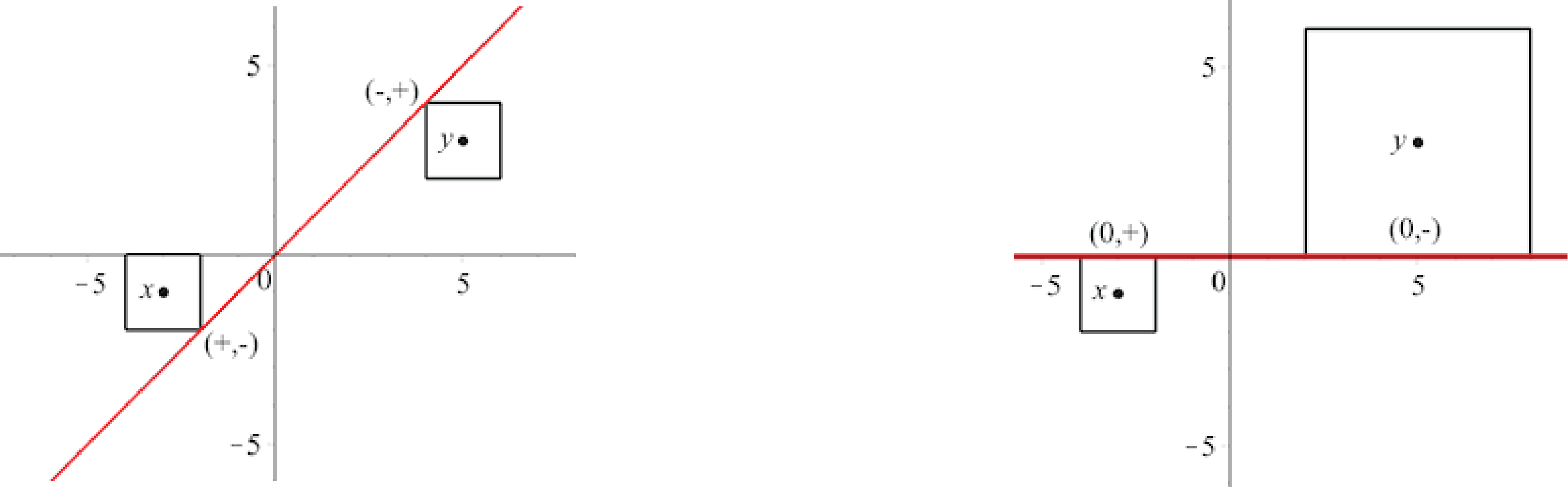
We will see that the sign vectors that can arise as the type of a point with respect to $L$ are precisely the elements of the oriented matroid associated to $L$. To aid in the proof we introduce the following convention for generating a vector with a given sign signature.

As we show in the following theorem, the dimension of $C(x,L)$ depends entirely on $\textnormal{type}_{L}(x)$. For any $\sigma\in\mathcal{O}_{L}$, the rank of $\sigma$ in $\mathcal{O}_{L}$, denoted $\textnormal{rank}(\sigma)$, is the rank of the support of $\sigma$ in the matroid underlying $\mathcal{O}_{L}$. So $\textnormal{rank}(\sigma)$ is the smallest number $k$ such that there exists indices $i_{1},\dots,i_{k}$ with $\sigma_{i_{j}}\neq 0$ such that for all $y\in L$, if $y_{i_{1}}=\dots=y_{i_{k}}=0$, then $y_{j}=0$ for $\sigma_{j}\neq 0$.

We can use the structure of the matroid $\mathcal{M}_{L}$ to glean information about possible values of $\dim(C(x,L))$. Let $U_{d,m}$ denote the uniform matroid of rank $d$ on ground set $\{1,\dots,m\}$; that is, the circuits of $U_{d,m}$ are all $d+1$-element subsets of $\{1,\dots,m\}$.

Lemma 2.6 enables us to give a partition of $\mathbb{R}^{m}$ by type with respect to $L$.

Modulo the lineality space $L$, the closures of the cones in Proposition 2.9 form the face fan of the zonotope obtained by projecting the cube $C_{d(x,L)}(x)$ onto $L^{\perp}$.

Let $RP(n)$ be the set of all $n$-leaf rooted trees with leaves labeled by $[n]:=\{1,\ldots,n\}$. Following the convention of [10, Section 2.2], we call the elements of $RP(n)$ rooted phylogenetic $[n]$-trees. We will also consider the set of rooted binary phylogenetic $[n]$-trees which we will denote $RB(n)$. A polytomy of a non-binary tree is a vertex with degree greater than three - that is, a witness to the property of being non-binary. To represent the topology of $\mathcal{T}\in RP(n)$ we use the notation $(S_{1}(S_{2}))$ to indicate that the leaves labeled by the set $S_{1}$ and $S_{2}$ are on opposite sides of the root in $\mathcal{T}$. We apply this notation recursively to give the topology of the rooted subtree in $\mathcal{T}$ induced by the labels in $S_{1}$ and $S_{2}$. Thus, for example, we can express the topology of the the rooted tree in Figure 4 by $(D(C(AB))).$

Let $\mathcal{T}\in RP(n)$ and assign a positive weighting to the edges of $\mathcal{T}$. This naturally induces a metric $\delta$ on the leaves of $\mathcal{T}$ where $\delta(i,j)$ is the sum of the edge weights on the unique path between $i$ and $j$. If we further assume that the distance from each leaf vertex to the root is the same then $\delta$ is an ultrametric.

An equidistant edge weighting of a rooted tree is a weighting of the edges where the distance from each leaf to the root is the same and where the weight of every internal edge is positive. Note that this allows the possibility of nonpositive weights on leaf edges. Given any ultrametric $u$ on $[n]$, there exists a unique $\mathcal{T}\in RP(n)$ and an equidistant weighting $w$ such that the ultrametric induced by $(\mathcal{T}:w)$ is equal to $u$ [10, Theorem 7.2.8]. We call $(\mathcal{T}:w)$ an equidistant representation of $u$ and say that $\mathcal{T}(u):=\mathcal{T}$ is the topology of $u$.

We can also convert an equidistant edge weighting of a tree into a vertex weighting of that same tree [10, Theorem 7.2.8]. Given any internal vertex $v$ in an equidistant representation of an ultrametric $u$, $u(i,j)$ is constant over all pairs of leaves $i,j$ having $v$ as their most recent common ancestor. We obtain a vertex weighting from an edge weighting by labeling each internal vertex by this constant value. For what follows, we will represent dissimilarity maps on $n$ elements as points in $\mathbb{R}^{n\choose 2}$ by letting $\delta_{ij}=\delta(i,j)$ and use $U_{n}\subseteq\mathbb{R}^{n\choose 2}$ to denote the set of all ultrametrics on $n$ elements. Many of our examples will involve dissimilarity maps on $4$ elements, in which case we let $(x_{AB},x_{AC},x_{AD},x_{BC},x_{BD},x_{CD})$ be the coordinates of an arbitrary point in $\mathbb{R}^{4\choose 2}$. We will also use the notation $e_{ij}$ to denote the standard basis vector with $x_{ij}=1$ and all other entries equal to zero.

Given a dissimilarity map $\delta$, we let $\delta_{U}$ be the unique coordinate-wise maximum ultrametric which is coordinate-wise less than $\delta$. This is called the subdominant ultrametric of $\delta$. The existence and uniqueness of the subdominant ultrametric are proven and a polynomial time algorithm for computing it is given in [10, Chapter 7].

Our interest in the subdominant ultrametric is that it gives us a way to determine an $l^{\infty}$-closest ultrametric to a dissimilarity map $\delta$ [5]. We first compute the subdominant ultrametric $\delta_{U}$ and then use that

We define $\delta_{c}$, the canonical closest ultrametric to $\delta$, by $\delta_{c}(i,j)=\delta_{U}(i,j)+\frac{1}{2}d(\delta,\delta_{U})$.

As noted in the introduction, the set of $l^{\infty}$-closest ultrametrics is in general not a single point. Moreover, in many instances, the set of $l^{\infty}$-closest ultrametrics to $\delta$, $C(\delta,U_{n})$, will contain ultrametrics representing different topologies. Thus, there may be several different trees that explain the data equally well from the perspective of the $l^{\infty}$-metric.

Example 3.3 shows that it is possible for the set of $l^{\infty}$-closest ultrametrics to a point to contain different topologies. Below, we consider what sets of topologies are represented in $C(\delta,U_{n})$ for an arbitrary point $\delta\in\mathbb{R}^{n\choose 2}$. The idea behind most of these proofs is to find a linear space that contains the ultrametrics for many different tree topologies and apply the constructions for linear spaces developed in Section 2.

In [6], the authors study the geometry of the set of dissimilarity maps around a polytomy with respect to the Euclidean norm. They showed that locally this space could be partitioned according to the closest tree topology. Proposition 3.5 shows the contrast between that situation and using the $l^{\infty}$-metric.

We obtain the following corollary by choosing a tree with a single resolved triple in the proof of Proposition 3.5.

We will also see from our decomposition of $\mathbb{R}^{4\choose 2}$ that there are actually 6-dimensional polyhedral cones in which every point in the interior has five $l^{\infty}$-closest binary tree topologies.
Even when all $l^{\infty}$-closest ultrametrics to some given $\delta\in\mathbb{R}^{\binom{n}{2}}$ have the same topology, the dimension of the set of $l^{\infty}$-closest ultrametrics can be high. The affine hull of each maximal cone of $U_{n}$ is a linear space defined by relations of the form $x_{ik}-x_{jk}=0$ where $(k(ij))$ is a triple compatible with the corresponding tree. As before, we can find points where optimizing to $U_{n}$ is equivalent to optimizing to such a linear space and so our results from Section 2 can be applied.

References

- [1] Maple 2015. Maplesoft, a division of Waterloo Maple Inc. Waterloo, Ontario.
- [2] Richa Agarwala, Vineet Bafna, Martin Farach, Mike Paterson, and Mikkel Thorup. On the approximability of numerical taxonomy (fitting distances by tree metrics). SIAM Journal on Computing, 28(3):1073–1085, 1998.
- [3] Federico Ardila. Subdominant matroid ultrametrics. Annals of Combinatorics, 8:379–389, 2004.
- [4] Federico Ardila and Caroline J. Klivans. The Bergman complex of a matroid and phylogenetic trees. Journal of Combinatorial Theory, Series B, 96(1):38 – 49, 2006.
- [5] V. Chepoi and B. Fichet. -approximation via subdominants. Journal of Mathematical Psychology, 44:600–616, 2000.
- [6] Ruth Davidson and Seth Sullivant. Distance-based phylogenetic algorithms around a tritomy. IEEE/ACM Transactions in Computational Biology and Bioinformatics, 11:325–335, 2014.
- [7] Bo Lin, Bernd Sturmfels, Xiaoxian Tang, and Ruriko Yoshida. Convexity in tree spaces. https://arxiv.org/abs/1510.08797, 2016.
- [8] Bo Lin and Ruriko Yoshida. Tropical Fermat-Weber points. https://arxiv.org/abs/1604.04674, 2016.
- [9] James Oxley. Matroid Theory. Oxford University Press, second edition, 2011.
- [10] Charles Semple and Mike Steel. Phylogenetics. Oxford University Press, Oxford, 2003.
- [11] David Speyer and Bernd Sturmfels. The tropical Grassmannian. Adv. Geom., 4:389–411, 2004.
- [12] Günter Ziegler. Lectures on Polytopes. Springer, 2000.