跳到论文正文
W Papers独立论文阅读器 arXiv:1702.05113 论文正文 计算阅读时间 · 0%
引用这篇论文根据当前论文元数据生成,正式投稿前建议核对。


License: arXiv.org perpetual non-exclusive license
arXiv:1702.05113v2 [math.ST] 24 Jun 2018

Adaptive Risk Bounds in Univariate Total Variation Denoising and Trend Filtering

Adityanand Guntuboyina??    Donovan Lieu    Sabyasachi Chatterjee    Bodhisattva Sen??
Abstract

We study trend filtering, a relatively recent method for univariate nonparametric regression. For a given integer r≥1r\geq 1, the rt​hr^{th} order trend filtering estimator is defined as the minimizer of the sum of squared errors when we constrain (or penalize) the sum of the absolute rt​hr^{th} order discrete derivatives of the fitted function at the design points. For r=1r=1, the estimator reduces to total variation regularization which has received much attention in the statistics and image processing literature. In this paper, we study the performance of the trend filtering estimator for every r≥1r\geq 1, both in the constrained and penalized forms. Our main results show that in the strong sparsity setting when the underlying function is a (discrete) spline with few “knots”, the risk (under the global squared error loss) of the trend filtering estimator (with an appropriate choice of the tuning parameter) achieves the parametric n−1n^{-1}-rate, up to a logarithmic (multiplicative) factor. Our results therefore provide support for the use of trend filtering, for every r≥1r\geq 1, in the strong sparsity setting.

keywords
Adaptive splines, discrete splines, fat shattering, higher order total variation regularization, metric entropy bounds, nonparametric function estimation, risk bounds, subdifferential, tangent cone

, , ,  and

423 Evans Hall
Berkeley, CA 94720
??
E-mail:

367 Evans Hall
Berkeley, CA 94720
??
E-mail:

117 Illini Hall
725 S. Wright St. M/C 374
Champaign, IL 61820
??

1255 Amsterdam Avenue
New York, NY 10027
??

1 Introduction

Consider the nonparametric regression problem where we observe data generated according to the model:

Yi=f∗(i/n)+ξi,i=1,…,n,Y_{i}=f^{*}({i}/{n})+\xi_{i},\qquad i=1,\ldots,n, (1)

where f∗:[0,1]→ℝf^{*}:[0,1]\to{\mathbb{R}} is the unknown regression function, and ξ1,…,ξn\xi_{1},\ldots,\xi_{n} are unobserved independent errors having the normal distribution with mean zero and variance σ2\sigma^{2}. The goal is to recover the underlying function f∗f^{*} from the measurements Y1,…,YnY_{1},\dots,Y_{n}. Alternatively, in the Gaussian sequence formulation, (1) can be expressed as

Y=θ∗+ξ,Y=\theta^{*}+\xi, (2)

where ξ∼Nn​(0,σ2​In)\xi\sim N_{n}(0,\sigma^{2}I_{n}), and θ∗:=(f∗​(1/n),f∗​(2/n),…,f∗​(1))\theta^{*}:=(f^{*}({1}/{n}),f^{*}({2}/{n}),\ldots,f^{*}(1)) is unknown. Here Nn​(0,σ2​In)N_{n}(0,\sigma^{2}I_{n}) denotes the multivariate normal distribution with mean vector zero and covariance matrix σ2​In\sigma^{2}I_{n}.

In this paper, we study the performance of trend filtering, a relatively new method for nonparametric regression with special emphasis on its risk properties. For a given integer r≥1r\geq 1, the rt​hr^{th} order trend filtering estimator is defined as the minimizer of the sum of squared errors when we constrain or penalize the sum of the absolute rt​hr^{th} order discrete derivatives of the fitted function at the design points. Formally, given a fixed integer r≥1r\geq 1 and a tuning parameter V≥0V\geq 0, the rt​hr^{th} order trend filtering estimator for θ∗\theta^{*} in the constrained form is given by

θ^V(r):=argminθ∈ℝn{12​‖Y−θ‖2:‖D(r)​θ‖1≤V​n1−r}\hat{\theta}^{(r)}_{V}:=\mathop{\rm argmin}_{\theta\in{\mathbb{R}}^{n}}\left\{\frac{1}{2}\|Y-\theta\|^{2}:\|D^{(r)}\theta\|_{1}\leq Vn^{1-r}\right\} (3)

where V>0V>0 is a tuning parameter (the multiplicative factor n1−rn^{1-r} is just for normalization), D(0)​θ:=θD^{(0)}\theta:=\theta, D(1)​θ:=(θ2−θ1,…,θn−θn−1)D^{(1)}\theta:=(\theta_{2}-\theta_{1},\dots,\theta_{n}-\theta_{n-1}) and D(r)​θD^{(r)}\theta, for r≥2r\geq 2, is recursively defined as D(r)​θ:=D(1)​(D(r−1)​θ)D^{(r)}\theta:=D^{(1)}(D^{(r-1)}\theta). Also ∥⋅∥1\|\cdot\|_{1} denotes the usual L1L^{1} norm defined by ‖x‖1:=∑i=1k|xi|\|x\|_{1}:=\sum_{i=1}^{k}|x_{i}| for x=(x1,…,xk)∈ℝkx=(x_{1},\dots,x_{k})\in{\mathbb{R}}^{k}. Note that ‖D(r)​θ‖1\|D^{(r)}\theta\|_{1} also equals V⁡(D(r−1)​θ)V(D^{(r-1)}\theta) where V⁡(α):=∑i=2k|αi−αi−1|V(\alpha):=\sum_{i=2}^{k}|\alpha_{i}-\alpha_{i-1}| denotes the variation of a vector α=(α1,…,αk)∈ℝk\alpha=(\alpha_{1},\ldots,\alpha_{k})\in{\mathbb{R}}^{k}. For simplicity, we denote the operator D(1)D^{(1)} by simply DD.

Alternatively, the trend filtering estimator in the penalized form is

θ^λ(r):=argminθ∈ℝn(12​‖Y−θ‖2+σ​nr−1​λ​‖D(r)​θ‖1)\hat{\theta}^{(r)}_{\lambda}:=\mathop{\rm argmin}_{\theta\in{\mathbb{R}}^{n}}\left(\frac{1}{2}\|Y-\theta\|^{2}+\sigma n^{r-1}\lambda\|D^{(r)}\theta\|_{1}\right) (4)

for r≥1r\geq 1 and tuning parameter λ≥0\lambda\geq 0. There is an abuse of notation here in that we are using the same notation for both the constrained and the penalized estimators. It may be noted, however, that when the subscript of θ^(r)\hat{\theta}^{(r)} is VV, we are referring to the constrained estimator (3) while when the subscript is λ\lambda, we are referring to the penalized estimator (4).

For r=1r=1, (4) reduces to the one-dimensional discrete version of total variation regularization or total variation denoising which was first proposed by Rudin, Osher and Fatemi [42] and has since been heavily used in the image processing community. The penalized estimator (4), for general r≥1r\geq 1, was first proposed by Steidl, Didas and Neumann [44] in the image processing literature who termed it higher order total variation regularization. The same estimator was later rediscovered by Kim et al. [25] who coined the name trend filtering for it. Many properties of the estimator have been studied in Tibshirani [46] and Wang, Smola and Tibshirani [51]. It should also be mentioned here that a continuous version of (4), where the discrete differences are replaced by continuous derivatives, was proposed much earlier in the statistics literature by Mammen and van de Geer [31] under the name locally adaptive regression splines.

The presence of the L1L^{1} norm in the constraint in (3) (resp. penalty in (4)) promotes sparsity of the vector D(r)​θ^V(r)D^{(r)}\hat{\theta}^{(r)}_{V} (resp. D(r)​θ^λ(r)D^{(r)}\hat{\theta}^{(r)}_{\lambda}). Now for every vector θ∈ℝn\theta\in{\mathbb{R}}^{n}, ‖D(r)​θ‖0=k\|D^{(r)}\theta\|_{0}=k if and only if θ\theta equals (f⁡(1/n),…,f⁡(n/n))(f(1/n),\dots,f(n/n)) for a discrete spline function ff that is made of k+1k+1 polynomials each of degree (r−1)(r-1) (here ‖x‖0\|x\|_{0} denotes the number of entries of the vector xx that are non-zero). Discrete splines are piecewise polynomials with regularity at the knots. They differ from the usual (continuous) splines in the form of the regularity condition at the knots: for splines, the regularity condition translates to (higher order) derivatives of adjacent polynomials agreeing at the knots, while for discrete splines it translates to discrete differences of adjacent polynomials agreeing at the knots; see Mangasarian and Schumaker [32] for details. This fact about the connection between ‖D(r)​θ‖0\|D^{(r)}\theta\|_{0} and discrete splines is standard (see e.g., Steidl, Didas and Neumann [44]) but we included a proof in Subsection D.3 for the convenience of the reader.

Thus the presence of the L1L^{1} norm in (3) (resp. (4)) implies that θ^V(r)\hat{\theta}^{(r)}_{V} (resp. θ^λ(r)\hat{\theta}^{(r)}_{\lambda}) can be written as (f^​(1/n),…,f^​(n/n))(\hat{f}(1/n),\dots,\hat{f}(n/n)) for a discrete spline f^\hat{f} of degree (r−1)(r-1) made up of not too many polynomial pieces. Trend filtering thus presents a way of fitting (discrete) splines to the data. Note that the knots of the discrete splines are automatically chosen by the optimization algorithms underlying (3) and (4) without any input from the user (except for the value of the tuning parameter VV or λ\lambda). Because of this automatic selection of the knots, trend filtering can be regarded as a spatially adaptive method (in the terminology of Donoho and Johnstone [9]). Note that such spatial adaptation is not exhibited by classical nonparametric regression methods such as local polynomials, kernels and splines, with a fixed tuning parameter. On the other hand, methods such as CART (Breiman et al. [4]), MARS (Friedman [14]), variable-bandwidth kernel/spline methods (see e.g., Müller and Stadtmüller [33], Brockmann, Gasser and Herrmann [5], Pintore, Speckman and Holmes [36] and Zhou and Shen [54]) and wavelets (Donoho and Johnstone [9]) are also spatially adaptive.

The present paper studies the performance of the estimators θ^V(r)\hat{\theta}_{V}^{(r)} and θ^λ(r)\hat{\theta}_{\lambda}^{(r)} as estimators of θ∗\theta^{*} under the multivariate Gaussian model (2). We shall use the squared error loss under which the risk of an estimator θ^\hat{\theta} is defined as

R⁡(θ^,θ∗):=1n​𝔼θ∗​‖θ^−θ∗‖2.R(\hat{\theta},\theta^{*}):=\frac{1}{n}{\mathbb{E}}_{\theta^{*}}\big\|\hat{\theta}-\theta^{*}\big\|^{2}. (5)

Under natural sparsity assumptions on θ∗\theta^{*}, we provide upper bounds on the risks R⁡(θ^V(r),θ∗)R(\hat{\theta}_{V}^{(r)},\theta^{*}) and R⁡(θ^λ(r),θ∗)R(\hat{\theta}_{\lambda}^{(r)},\theta^{*}) as well as high probability upper bounds on the random loss functions ‖θ^V(r)−θ∗‖2/n\|\hat{\theta}_{V}^{(r)}-\theta^{*}\|^{2}/n and ‖θ^λ(r)−θ∗‖2/n\|\hat{\theta}_{\lambda}^{(r)}-\theta^{*}\|^{2}/n.

It is natural to study the risk properties of (3) and (4) under the following two kinds of assumptions on θ∗\theta^{*}: (a) nr−1​‖D(r)​θ∗‖1≤Vn^{r-1}\|D^{(r)}\theta^{*}\|_{1}\leq V for some V>0V>0 (possibly dependent on nn), and (b) ‖D(r)​θ∗‖0≤k\|D^{(r)}\theta^{*}\|_{0}\leq k for some kk that is much smaller than nn. We shall refer to these two regimes as weak sparsity and strong sparsity respectively. This breakdown into weak and strong sparsity settings is inspired by corresponding terminology in the study of risk properties of thresholding based estimators in Gaussian sequence models [24] and the prediction risk properties of the LASSO estimators in regression [6]. Indeed, as demonstrated in Tibshirani [46], there is a close connection between the trend filtering estimators and LASSO (more details are provided in Subsection 5.4).

A thorough study on the performance of the penalized trend filtering estimator (4) under weak sparsity has been done by Tibshirani [46] and Wang, Smola and Tibshirani [51] building on earlier results of Mammen and van de Geer [31]. It is proved there that, when the tuning parameter λ\lambda is appropriately chosen, the penalized estimator (4) is minimax optimal in the weak sparsity setting. Actually, the weak sparsity results of [46, 51] are broader and hold under more general settings (see Remark 2.1 for more details).

The present paper focuses on the strong sparsity setting. Compared to available results in the weak sparsity setting, relatively little is known about the performance of the trend filtering estimators in the strong sparsity setting. In fact, all existing results [8, 30, 34, 48, 29, 21] for strong sparsity deal with the case r=1r=1 (where trend filtering is the same as total variation denoising). To the best of our knowledge, the present paper is the first to prove risk bounds for trend filtering under strong sparsity for arbitrary r≥1r\geq 1. We also improve, in certain aspects, existing results for r=1r=1.

In order to motivate our results, let us consider the strong sparsity setting where it is assumed that D(r)​θ∗D^{(r)}\theta^{*} is sparse. If ‖D(r)​θ∗‖0=k\|D^{(r)}\theta^{*}\|_{0}=k, then, as mentioned previously, θ∗=(f⁡(1/n),…,f⁡((n−1)/n),f⁡(1))\theta^{*}=(f(1/n),\dots,f((n-1)/n),f(1)) for a discrete spline function ff that is made of k+1k+1 polynomials each of degree (r−1)(r-1). Given data Y∼Nn​(θ∗,σ2​In)Y\sim N_{n}(\theta^{*},\sigma^{2}I_{n}), an oracle piecewise polynomial estimator (having access to locations of the knots of θ∗\theta^{*}) would put knots corresponding to θ∗\theta^{*} and then fit a polynomial of degree (r−1)(r-1) in each of the partitions given by the knots. This would be a linear estimator with at most (k+1)​r(k+1)r degrees vvof freedom and its risk (defined as in (5)) will be bounded by r​σ2​(k+1)/nr\sigma^{2}(k+1)/n. This motivates the following question which is the focus of this paper: When ‖D(r)​θ∗‖0=k\|D^{(r)}\theta^{*}\|_{0}=k, how do the risks of properly tuned trend filtering estimators (3) and (4) compare with the oracle risk of r​σ2​(k+1)/nr\sigma^{2}(k+1)/n?

The main results of this paper for constrained trend filtering (Theorem 2.2 and Corollary 2.3) imply that when ‖D(r)​θ∗‖0=k\|D^{(r)}\theta^{*}\|_{0}=k, the risk of θ^V(r)\hat{\theta}^{(r)}_{V} satisfies

R⁡(θ^V(r),θ∗)≤Cr​(c)​σ2​k+1n​log⁡e​nk+1,R(\hat{\theta}^{(r)}_{V},\theta^{*})\leq C_{r}(c)\sigma^{2}\frac{k+1}{n}\log\frac{en}{k+1}, (6)

provided

  1. (i)

    the tuning parameter VV is non-random and close to V∗:=nr−1​‖D(r)​θ∗‖1V^{*}:=n^{r-1}\|D^{(r)}\theta^{*}\|_{1}, and

  2. (ii)

    (minimum length condition) each of the polynomial pieces of θ∗\theta^{*} have length bounded below by c​n/(k+1)cn/(k+1) for a constant c>0c>0 (in fact, our result requires a weaker version of this condition; see (13) and Remark 2.4).

Here Cr​(c)C_{r}(c) is a positive constant that depends only on rr and the constant cc from the second assumption above.

We also prove results for the penalized estimators. For r=1r=1, our main result (Corollary 2.8) states that the risk of θ^λ(1)\hat{\theta}^{(1)}_{\lambda} is also bounded by the right hand side of (6) under the minimum length condition provided λ\lambda is close to a theoretical choice λ∗\lambda^{*} and λ≥λ∗\lambda\geq\lambda^{*}. This choice λ∗\lambda^{*} depends on θ∗\theta^{*} and is defined in (27). We provide an explicit upper bound for λ∗\lambda^{*} in Lemma 2.9 which gives risk bounds for θ^λ(1)\hat{\theta}^{(1)}_{\lambda} under more explicit choices of λ\lambda (see Corollary 2.10). A comparison of these results to existing results is given in Remarks 2.6 and 2.7.

For r≥2r\geq 2, we prove, in Corollary 2.11, that the penalized estimator satisfies

R⁡(θ^λ(r),θ∗)≤Cr​(c)​σ2​(k+1n​log⁡e​nk+1+(k+1)2​rn)R(\hat{\theta}^{(r)}_{\lambda},\theta^{*})\leq C_{r}(c)\sigma^{2}\left(\frac{k+1}{n}\log\frac{en}{k+1}+\frac{(k+1)^{2r}}{n}\right) (7)

under the minimum length condition provided that λ\lambda is close to λ∗\lambda^{*} (defined in (27)) and λ≥λ∗\lambda\geq\lambda^{*}. Explicit upper bounds for λ∗\lambda^{*} are in Lemma 2.12 and risk bounds for θ^λ(r)\hat{\theta}^{(r)}_{\lambda} with explicit penalty choices are in Corollary 2.13. Note that (7) is weaker compared to (6) in terms of the dependence on kk.

The implication of our results is the following. As mentioned earlier, the trend filtering estimators are given by discrete spline functions of degree r−1r-1. The knots of these splines are chosen automatically by the algorithm (the user only needs to specify the tuning parameter VV or λ\lambda). Our results indicate that under the assumption ‖D(r)​θ∗‖0=k\|D^{(r)}\theta^{*}\|_{0}=k (i.e., θ∗\theta^{*} is a discrete spline of degree r−1r-1 with k+1k+1 polynomial pieces) with a minimum length condition on the polynomial pieces of θ∗\theta^{*}, the automatic selection of knots by the trend filtering estimators (when appropriate choices of VV or λ\lambda) happens in a way that the overall risk is comparable to the oracle risk of r​σ2​(k+1)/nr\sigma^{2}(k+1)/n. In fact, when k=O⁡(1)k=O(1), the risks of the ideally tuned trend filtering estimators is only off compared to the oracle risk by a factor that is logarithmic in nn (we also prove in Lemma 2.4 that this logarithmic factor cannot be completely removed in general). The automatic knot selection of trend filtering can therefore be interpreted as being done adaptively depending on the structure of the unknown θ∗\theta^{*} in order to approximate the oracle risk. This is the reason why we refer to our results as adaptive risk bounds. It should be mentioned here that a similar adaptation story can also be used to describe the weak sparsity results [46, 51] where the knots are adaptively chosen to attain the minimax rate under the L1L^{1} constraint on D(r)​θ∗D^{(r)}\theta^{*}. Therefore, our results (together with those of [46, 51]) provide support for the use of the trend filtering estimators in both weak and strong sparsity settings.

We would like to mention here that theoretical analysis of spatially adaptive nonparametric regression methods under strong sparsity is non-trivial. Indeed, among various such methods including CART, MARS, variable-bandwidth kernel/spline methods and wavelets, rigorous theoretical risk results under strong sparsity only exist for wavelets [9] and variable-bandwidth kernel methods [28, 17]. The analysis of trend filtering estimators is more involved compared to estimators based on wavelets and variable-bandwidth kernels because the trend filtering estimators are given by the output of an optimization algorithm and have no closed form expressions.

The rest of this paper is organized as follows. Our main results are described in Section 2: Subsection 2.1 deals with the constrained estimator where we provide risk bounds under both weak sparsity (which was not known previously) and strong sparsity. Subsection 2.2 deals with the penalized estimator and here we separate our presentation into two parts: results for r=1r=1 and results for r≥2r\geq 2; our results for r≥2r\geq 2 are weaker (there is an additional (k+1)2​r/n(k+1)^{2r}/n term in the risk) than the results for r=1r=1. Throughout, we focus on nonasymptotic upper bounds for the risk (expected loss) although all our results can be converted into high probability upper bounds on the loss (see Remark 2.3). All proofs are given in the supplementary material at the end of the paper and a high level overview of the proofs is provided in Section 3. Section 4 contains some simulation studies supporting some of our theoretical results. Finally several interesting issues related to our results are described in Section 5.

2 Main Results

Throughout CrC_{r} will denote a positive constant that depends on rr alone although its precise value will change from equation to equation. We shall assume that n≥2​rn\geq 2r throughout the paper (many of our results also hold under the weaker condition n≥r+1n\geq r+1).

2.1 Results for the Constrained Estimator

We start with the bound of n−2r/(2r+1)n^{-2r/(2r+1)} for risk of θ^V(r)\hat{\theta}^{(r)}_{V} under the condition that the tuning parameter VV satisfies ‖D(r)​θ∗‖1≤V​n1−r\|D^{(r)}\theta^{*}\|_{1}\leq Vn^{1-r}. This result is similar to results in Mammen and van de Geer [31], Tibshirani [46] and Wang, Smola and Tibshirani [51] who focussed on the penalized estimator (4) (see Remark 2.1 for details). We also explicitly state the dependence of the bound on VV and σ\sigma.

Theorem 2.1.

Fix r≥1r\geq 1. Suppose that the tuning parameter VV is chosen so that nr−1​‖D(r)​θ∗‖1≤Vn^{r-1}\|D^{(r)}\theta^{*}\|_{1}\leq V. Then there exists a positive constant CrC_{r} depending on rr alone such that

R⁡(θ^V(r),θ∗)≤Cr​max⁡((σ2​V1/rn)2​r/(2​r+1),σ2n​log⁡(e​n)).R(\hat{\theta}^{(r)}_{V},\theta^{*})\leq C_{r}\max\left(\left(\frac{\sigma^{2}V^{1/r}}{n}\right)^{2r/(2r+1)},\frac{\sigma^{2}}{n}\log(en)\right). (8)

Also for every x>0x>0, we have

1n​‖θ^V(r)−θ∗‖2≤Cr​max⁡((σ2​V1/rn)2​r/(2​r+1),σ2n​log⁡(e​n))+4​σ2​xn\frac{1}{n}\|\hat{\theta}^{(r)}_{V}-\theta^{*}\|^{2}\leq C_{r}\max\left(\left(\frac{\sigma^{2}V^{1/r}}{n}\right)^{2r/(2r+1)},\frac{\sigma^{2}}{n}\log(en)\right)+\frac{4\sigma^{2}x}{n} (9)

with probability at least 1−e−x1-e^{-x}.

Remark 2.1.

As mentioned earlier, bounds similar to (8) and (9) have been proved in Mammen and van de Geer [31], Tibshirani [46] and Wang, Smola and Tibshirani [51] for the penalized trend filtering estimator. Actually, the bounds in these earlier papers hold under more general assumptions than the assumptions of the current paper. For example, their analyses also holds under the assumption that the (continuous) variation norm of the function (f∗)(r−1)(f^{*})^{(r-1)} (this is the (r−1)t​h(r-1)^{th} derivative of f∗f^{*}) is at most VV, where f∗f^{*} is the true function with θ∗=(f∗​(1/n),…,f∗​(1))\theta^{*}=(f^{*}(1/n),\dots,f^{*}(1)). Note that there is subtle difference between this and our assumption of an upper bound on ‖D(r)​θ∗‖1\|D^{(r)}\theta^{*}\|_{1} in the sequence model (2). An assumption on the variation norm of (f∗)(r−1)(f^{*})^{(r-1)} does not directly lead to a bound on ‖D(r)​θ∗‖1\|D^{(r)}\theta^{*}\|_{1} which makes the analysis difficult (see Wang, Smola and Tibshirani [51] for more details on the relation between the two variation norms). Also, the results in these earlier papers studied the general setting with θ∗:=(f∗​(x1),…,f∗​(xn))\theta^{*}:=(f^{*}(x_{1}),\dots,f^{*}(x_{n})) where x1,…,xnx_{1},\dots,x_{n} are design points that are not necessarily equally spaced. We restrict ourselves to the equally spaced design setting in this paper (see Subsection 5.1).

Remark 2.2.

n−2r/(2r+1)n^{-2r/(2r+1)} is the minimax rate of estimation over the class of θ∈ℝn\theta\in{\mathbb{R}}^{n} with ‖D(r)​θ‖1≤V​n1−r\|D^{(r)}\theta\|_{1}\leq Vn^{1-r} (see e.g., Donoho and Johnstone [10]). This means that the constrained trend filtering estimator with tuning parameter VV is minimax optimal over {θ∈ℝn:‖D(r)​θ‖1≤V​n1−r}\{\theta\in{\mathbb{R}}^{n}:\|D^{(r)}\theta\|_{1}\leq Vn^{1-r}\}. This result was known previously for the penalized estimator; see Tibshirani [46]. Note also that VV here can change with nn as well and inequality (8) implies that θ^V(r)\hat{\theta}_{V}^{(r)} is minimax optimal even in terms of the dependence of the rate on VV.

Before we state results for strong sparsity, we need some notation. Fix an integer r≥1r\geq 1 and let n≥r+1n\geq r+1. For a vector θ∈ℝn\theta\in{\mathbb{R}}^{n} and an index 2≤j≤n−r+12\leq j\leq n-r+1, we say that jj is an rt​hr^{th} order knot (or knot of order rr) of θ\theta provided (D(r−1)​θ)j−1≠(D(r−1)​θ)j(D^{(r-1)}\theta)_{j-1}\neq(D^{(r-1)}\theta)_{j}. Note that first order knots are just jumps and second order knots are points of change of slope. We also say that an rt​hr^{th} order knot jj has sign +1+1 if (D(r−1)​θ)j−1<(D(r−1)​θ)j(D^{(r-1)}\theta)_{j-1}<(D^{(r-1)}\theta)_{j} and sign −1-1 if (D(r−1)​θ)j−1>(D(r−1)​θ)j(D^{(r-1)}\theta)_{j-1}>(D^{(r-1)}\theta)_{j}. For θ∈ℝn\theta\in{\mathbb{R}}^{n}, we let

𝐤r​(θ):=‖D(r)​θ‖0​ and ​V(r)​(θ):=nr−1​‖D(r)​θ‖1.{\mathbf{k}_{r}}(\theta):=\|D^{(r)}\theta\|_{0}~~~\text{ and }~~~V^{(r)}(\theta):=n^{r-1}\|D^{(r)}\theta\|_{1}. (10)

When r=1r=1, note that V(1)​(θ)=‖D​θ‖1=|θ2−θ1|+⋯+|θn−θn−1|V^{(1)}(\theta)=\|D\theta\|_{1}=|\theta_{2}-\theta_{1}|+\dots+|\theta_{n}-\theta_{n-1}| which is simply the variation of θ\theta. We therefore simply denote V(1)​(θ)V^{(1)}(\theta) by V⁡(θ)V(\theta). It also follows then that V(r)​(θ)=nr−1​V​(D(r−1)​θ)V^{(r)}(\theta)=n^{r-1}V(D^{(r-1)}\theta).

It may be observed that 𝐤r​(θ){\mathbf{k}_{r}}(\theta) equals precisely the number of rt​hr^{th} order knots of θ\theta. When the value of rr and θ∈ℝn\theta\in{\mathbb{R}}^{n} are clear from the context, we simply denote 𝐤r​(θ){\mathbf{k}_{r}}(\theta) by kk. Also, note that as D(r)​θD^{(r)}\theta is a vector of length n−rn-r, we necessarily have 𝐤r​(θ)=‖D(r)​θ‖0≤n−r≤n−1{\mathbf{k}_{r}}(\theta)=\|D^{(r)}\theta\|_{0}\leq n-r\leq n-1.

Suppose 𝐤r​(θ)=k{\mathbf{k}_{r}}(\theta)=k and let 2≤j1<⋯<jk≤n−r+12\leq j_{1}<\dots<j_{k}\leq n-r+1 denote all the rt​hr^{th} order knots of θ\theta with associated signs 𝔯1,…,𝔯k∈{−1,1}{\mathfrak{r}}_{1},\dots,{\mathfrak{r}}_{k}\in\{-1,1\}. Also let 𝔯0=𝔯k+1=0{\mathfrak{r}}_{0}={\mathfrak{r}}_{k+1}=0. Further, let n0:=j1+r−2n_{0}:=j_{1}+r-2, ni:=ji+1−jin_{i}:=j_{i+1}-j_{i}, for 1≤i≤k−11\leq i\leq k-1, and nk:=n−r+2−jkn_{k}:=n-r+2-j_{k}, and observe that ∑i=0kni=n\sum_{i=0}^{k}n_{i}=n. Finally, let

ni∗:=min(ni,nk+1)for i=0,1,…,k.n_{i*}:=\min\left(n_{i},\frac{n}{k+1}\right)\qquad\text{for $i=0,1,\dots,k$}.

We now define two quantities δr​(θ)\delta_{r}(\theta) and Δr​(θ)\Delta_{r}(\theta) in the following way:

δr(θ):=(n0∗1−2​r+nk∗1−2​r+∑i=1k−1ni∗1−2​rI{𝔯i≠𝔯i+1})1/2\delta_{r}(\theta):=\left(n^{1-2r}_{0*}+n^{1-2r}_{k*}+\sum_{i=1}^{k-1}n_{i*}^{1-2r}I\{{\mathfrak{r}}_{i}\neq{\mathfrak{r}}_{i+1}\}\right)^{1/2} (11)

and

Δr​(θ):=k+1n​log⁡e​nk+1+δr2​(θ)n​(nk+1)2​r−1​log⁡e​nk+1+(δr​(θ)n)1/r\Delta_{r}(\theta):=\frac{k+1}{n}\log\frac{en}{k+1}+\frac{\delta^{2}_{r}(\theta)}{n}\left(\frac{n}{k+1}\right)^{2r-1}\log\frac{en}{k+1}+\left(\frac{\delta_{r}(\theta)}{\sqrt{n}}\right)^{1/r} (12)

where, in the definition of δr​(θ)\delta_{r}(\theta), the quantity I{𝔯i≠𝔯i+1}I\{{\mathfrak{r}}_{i}\neq{\mathfrak{r}}_{i+1}\} denotes the indicator variable that equals 11 if 𝔯i≠𝔯i+1{\mathfrak{r}}_{i}\neq{\mathfrak{r}}_{i+1} and 00 if 𝔯i=𝔯i+1{\mathfrak{r}}_{i}={\mathfrak{r}}_{i+1}. Note that trivially Δr​(θ)≥(k+1)/n≥1/n\Delta_{r}(\theta)\geq(k+1)/n\geq 1/n.

Our results will show that the risk of the estimator θ^V(r)\hat{\theta}^{(r)}_{V} for θ∗\theta^{*} will essentially be controlled by Δr​(θ∗)\Delta_{r}(\theta^{*}). The key point to note about Δr​(θ)\Delta_{r}(\theta) is the fact (easy to check) that when

min0≤i≤k:𝔯i≠𝔯i+1ni≥c​nk+1\min_{0\leq i\leq k:{\mathfrak{r}}_{i}\neq{\mathfrak{r}}_{i+1}}n_{i}\geq\frac{cn}{k+1} (13)

for a positive constant c≤1c\leq 1 (here 𝔯1,…,𝔯k∈{−1,1}{\mathfrak{r}}_{1},\dots,{\mathfrak{r}}_{k}\in\{-1,1\} are the signs of the rt​hr^{th} order knots of θ\theta while 𝔯0{\mathfrak{r}}_{0} and 𝔯k+1{\mathfrak{r}}_{k+1} are taken to be zero), then

δr2​(θ)≤(c​nk+1)1−2​r​(k+1)\delta^{2}_{r}(\theta)\leq\left(\frac{cn}{k+1}\right)^{1-2r}(k+1)

and consequently

Δr​(θ)\displaystyle\Delta_{r}(\theta) ≤{1+c1−2​r}​k+1n​log⁡e​nk+1+c(1−2​r)/(2​r)​k+1n\displaystyle\leq\left\{1+c^{1-2r}\right\}\frac{k+1}{n}\log\frac{en}{k+1}+c^{(1-2r)/(2r)}\frac{k+1}{n}
≤{1+c1−2​r+c(1−2​r)/(2​r)}​k+1n​log⁡e​nk+1.\displaystyle\leq\left\{1+c^{1-2r}+c^{(1-2r)/(2r)}\right\}\frac{k+1}{n}\log\frac{en}{k+1}. (14)

We say that θ\theta satisfies the minimum length condition with constant cc if condition (13) holds. We have just observed that when θ\theta satisfies the minimum length condition with constant cc then Δr​(θ)≤Cr​(c)​k+1n​log⁡e​nk+1\Delta_{r}(\theta)\leq C_{r}(c)\frac{k+1}{n}\log\frac{en}{k+1} for a constant Cr​(c)C_{r}(c) depending only on cc and rr.

The following is our main result for the constrained trend filtering estimator.

Theorem 2.2.

Fix r≥1r\geq 1 and n≥2​rn\geq 2r. Consider the estimator θ^V(r)\hat{\theta}^{(r)}_{V} defined in (3) with tuning parameter V≥0V\geq 0. Then for every θ∗∈ℝn\theta^{*}\in{\mathbb{R}}^{n}, we have

R(θ^V(r),θ∗)≤infθ∈ℝn:V(r)​(θ)=V(1n∥θ∗−θ∥2+Crσ2Δr(θ))R(\hat{\theta}^{(r)}_{V},\theta^{*})\leq\inf_{\theta\in{\mathbb{R}}^{n}:V^{(r)}(\theta)=V}\left(\frac{1}{n}\|\theta^{*}-\theta\|^{2}+C_{r}\sigma^{2}\Delta_{r}(\theta)\right) (15)

for a positive constant CrC_{r}, depending only on rr.

Remark 2.3 (High-probability bound).

Note that Theorem 2.2 gives an upper bound for R⁡(θ^V(r),θ∗)R(\hat{\theta}^{(r)}_{V},\theta^{*}) which is the expectation of 1n​‖θ^V(r)−θ∗‖2\frac{1}{n}\|\hat{\theta}_{V}^{(r)}-\theta^{*}\|^{2}. Similarly as in Theorem 2.1, the risk bound (15) can be supplemented by the following high probability bound: for every x>0x>0, we have

1n∥θ^V(r)−θ∗∥2≤infθ∈ℝn:V(r)​(θ)=V(1n∥θ∗−θ∥2+Crσ2Δr(θ))+4​σ2​xn\frac{1}{n}\|\hat{\theta}_{V}^{(r)}-\theta^{*}\|^{2}\leq\inf_{\theta\in{\mathbb{R}}^{n}:V^{(r)}(\theta)=V}\left(\frac{1}{n}\|\theta^{*}-\theta\|^{2}+C_{r}\sigma^{2}\Delta_{r}(\theta)\right)+\frac{4\sigma^{2}x}{n} (16)

with probability at least 1−e−x1-e^{-x}. This will be true in all the results of this paper (namely that the bound on R⁡(θ^,θ∗)R(\hat{\theta},\theta^{*}) plus 4​σ2​x/n4\sigma^{2}x/n will dominate 1n​‖θ^−θ∗‖2\frac{1}{n}\|\hat{\theta}-\theta^{*}\|^{2} with probability at least 1−e−x1-e^{-x}). Thus, for ease of presentation, we shall omit high probability statements and only report risk results (i.e., bounds on R⁡(θ^,θ∗)R(\hat{\theta},\theta^{*})) in the rest of the paper.

Theorem 2.2 applies to every θ∗∈ℝn\theta^{*}\in{\mathbb{R}}^{n} and is stated in the sharp oracle form. It implies that the risk of θ^V(r)\hat{\theta}^{(r)}_{V} is small provided there exists some θ∈ℝn\theta\in{\mathbb{R}}^{n} with V(r)​(θ)=VV^{(r)}(\theta)=V such that (a) ‖θ−θ∗‖\|\theta-\theta^{*}\| is small, and (b) Δr​(θ)\Delta_{r}(\theta) is small.

Theorem 2.2 yields the following corollary which is a non-oracle inequality and is more readily interpretable. Recall from (14) that Δr​(θ)\Delta_{r}(\theta) is bounded from above by a constant multiple of k+1n​log⁡e​nk+1\frac{k+1}{n}\log\frac{en}{k+1} with 𝐤r​(θ)=k{\mathbf{k}_{r}}(\theta)=k provided θ\theta satisfies (13).

Corollary 2.3.

Consider the estimator θ^V(r)\hat{\theta}^{(r)}_{V} with tuning parameter VV. Suppose θ∗\theta^{*} satisfies the minimum length condition (13) with constant cc, then

R⁡(θ^V(r),θ∗)≤(V−V(r)​(θ∗))2+Cr​(c)​σ2​(𝐤r​(θ∗)+1)n​log⁡e​n𝐤r​(θ∗)+1R(\hat{\theta}^{(r)}_{V},\theta^{*})\leq\left(V-V^{(r)}(\theta^{*})\right)^{2}+C_{r}(c)\frac{\sigma^{2}\left({\mathbf{k}_{r}}(\theta^{*})+1\right)}{n}\log\frac{en}{{\mathbf{k}_{r}}(\theta^{*})+1} (17)

where Cr​(c)C_{r}(c) is a positive constant that depends on rr and cc alone. Further, if VV is chosen so that

(V−V(r)​(θ∗))2≤C​σ2​(𝐤r​(θ∗)+1)n​log⁡e​n𝐤r​(θ∗)+1\left(V-V^{(r)}(\theta^{*})\right)^{2}\leq C\frac{\sigma^{2}({\mathbf{k}_{r}}(\theta^{*})+1)}{n}\log\frac{en}{{\mathbf{k}_{r}}(\theta^{*})+1}

for a positive constant CC, then we have

R⁡(θ^V(r),θ∗)≤Cr​(c,C)​σ2​(𝐤r​(θ∗)+1)n​log⁡e​n𝐤r​(θ∗)+1R(\hat{\theta}^{(r)}_{V},\theta^{*})\leq C_{r}(c,C)\frac{\sigma^{2}\left({\mathbf{k}_{r}}(\theta^{*})+1\right)}{n}\log\frac{en}{{\mathbf{k}_{r}}(\theta^{*})+1} (18)

for a positive constant Cr​(c,C)C_{r}(c,C) that depends on rr, cc and CC alone.

Note that Theorem 2.2 and Corollary 2.3 both apply to every r≥1r\geq 1. On the other hand, existing adaptation results for trend filtering all deal with the case r=1r=1 (which corresponds to total variation regularization). Even for r=1r=1, our results are stronger, in some respects, compared to the existing results in the literature (see Remark 2.6 for a precise comparison).

Remark 2.4 (On the minimum length condition).

The minimum length condition (13) required for Corollary 2.3 is weaker than existing minimum length conditions in the literature (this comparison is only for r=1r=1 because no results exist for r≥2r\geq 2) which are all of the form

min0≤i≤k⁡ni≥c​nk+1where k=𝐤1​(θ∗).\min_{0\leq i\leq k}n_{i}\geq\frac{cn}{k+1}\qquad\text{where $k=\mathbf{k}_{1}(\theta^{*})$}. (19)

Indeed our condition (13) requires that ni≥c​n/(k+1)n_{i}\geq cn/(k+1) be true only for those ii for which 𝔯i≠𝔯i+1{\mathfrak{r}}_{i}\neq{\mathfrak{r}}_{i+1} while (19) requires this for all ii. To see why our condition can be substantially weaker, consider, for example, the situation when D(r−1)​θ∗D^{(r-1)}\theta^{*} is a monotonic vector (for r=1r=1, this means that θ∗\theta^{*} is itself monotone while for r=2r=2, this means that θ∗\theta^{*} is convex/concave). In this case, condition (13) is equivalent to requiring that ni≥c​n/(k+1)n_{i}\geq cn/(k+1) only for i=0i=0 and i=ki=k which is much weaker than requiring it for all 0≤i≤k0\leq i\leq k.

The fact that our minimum length condition involves only those ii for which 𝔯i≠𝔯i+1{\mathfrak{r}}_{i}\neq{\mathfrak{r}}_{i+1} as opposed to involving all i∈{0,1,…,k}i\in\{0,1,\dots,k\} is especially crucial for r≥2r\geq 2. To see this, consider the piecewise linear function f∗f^{*} on [0,1][0,1] shown in Figure 1. This function clearly has three knots (points of change of slope) in (0,1)(0,1). However the vector θ∗\theta^{*} obtained as (f∗​(1/n),…,f∗​(n/n))(f^{*}(1/n),\dots,f^{*}(n/n)) (with n=15n=15) has six second order knots. The reason for the additional knots is due to the fact that the original knots of f∗f^{*} are not at the design points 1/n,…,n/n1/n,\dots,n/n. Note however that because of these additional knots, the minimum length condition will not be satisfied over all i=0,1,…,ki=0,1,\dots,k. On the other hand, it should be clear that (13) will still be satisfied because the additional linear pieces satisfy the property that 𝔯i=𝔯i+1{\mathfrak{r}}_{i}={\mathfrak{r}}_{i+1}.

Fig 1: A piecewise linear function f∗f^{*} on [0,1][0,1] together with the vector θ∗:=(f∗​(1/n),…,f∗​(1))\theta^{*}:=(f^{*}(1/n),\dots,f^{*}(1)) for n=15n=15 plotted in red. Note that f∗f^{*} has three knots while θ∗\theta^{*} has six first order knots.
Remark 2.5 (The minimum length condition cannot be removed).

We shall argue here via simulations that the minimum length condition in Corollary 2.3 cannot be removed. Suppose that θ∗\theta^{*} is given by

θ1∗=⋯=θn−1∗=0​ and ​θn∗=5\theta_{1}^{*}=\dots=\theta_{n-1}^{*}=0~~~\text{ and }~~~\theta_{n}^{*}=5 (20)

and consider estimating θ∗\theta^{*} from an observation Y∼Nn​(θ∗,In)Y\sim N_{n}(\theta^{*},I_{n}) (i.e., σ=1\sigma=1) by θ^V(1)\hat{\theta}^{(1)}_{V} (i.e., r=1r=1) with tuning parameter V=V(1)​(θ∗)=5V=V^{(1)}(\theta^{*})=5. It is clear here that 𝐤1​(θ∗)=1\mathbf{k}_{1}(\theta^{*})=1. The minimum length condition (13) is not satisfied because n0=n−1n_{0}=n-1 and n1=1n_{1}=1. The risk R⁡(θ^V(1),θ∗)R(\hat{\theta}^{(1)}_{V},\theta^{*}) can be computed via simulation. In Figure 2 (left panel), we have plotted log⁡R⁡(θ^V(1),θ∗)\log R(\hat{\theta}^{(1)}_{V},\theta^{*}) against log⁡n\log n for values of nn between 1000 and 5000 (chosen to be equally spaced on the log-scale). For each value of nn, we calculated the risk using 100100 Monte Carlo replications. The slope of the least squares line through these points turned out to be close to −2/3-2/3 which indicates that the risk R⁡(θ^V(1),θ∗)R(\hat{\theta}^{(1)}_{V},\theta^{*}) decays at the rate n−2/3n^{-2/3}. This rate is slower than the rate given by Corollary 2.3 indicating that inequality (17) is not true for this θ∗\theta^{*}. On the other hand, the n−2/3n^{-2/3} rate here makes sense in light of Theorem 2.1. Therefore, even though the vector D​θ∗D\theta^{*} is sparse (with ‖D​θ∗‖0=1\|D\theta^{*}\|_{0}=1), the rate of convergence of θ^(1)\hat{\theta}^{(1)} is equal to the n−2/3n^{-2/3} and not the faster rate given by Corollary 2.3. This points to the necessity of the minimum length condition (13).

Refer to caption
Refer to caption
Fig 2: Left: plot of log⁡R⁡(θ^V(1),θ∗)\log R(\hat{\theta}^{(1)}_{V},\theta^{*}) against log⁡n\log n for θ∗\theta^{*} as in (20). The least squares slope is close to −2/3-2/3 which suggests that the risk decays as n−2/3n^{-2/3} instead of the faster rate given by Corollary 2.3. Right: plot of log⁡R⁡(θ^V(2),θ∗)\log R(\hat{\theta}^{(2)}_{V},\theta^{*}) against log⁡n\log n for θ∗\theta^{*} defined in (21). The slope is close to −2/5-2/5 which suggests that the risk decays as n−2/5n^{-2/5} instead of the faster rate given by Corollary 2.3.

Another counterexample for the necessity of (13) for Corollary 2.3 is:

θ1∗=⋯=θ⌊n/2⌋∗=0 and θ⌊n/2⌋+1∗=θ⌊n/2⌋+2∗=⋯=θn∗=5.\theta_{1}^{*}=\dots=\theta_{\lfloor n/2\rfloor}^{*}=0~~~\text{ and }~~~\theta_{\lfloor n/2\rfloor+1}^{*}=\theta_{\lfloor n/2\rfloor+2}^{*}=\dots=\theta_{n}^{*}=5. (21)

Here consider the problem of estimating θ∗\theta^{*} by the estimator θ^V(2)\hat{\theta}^{(2)}_{V} (i.e., r=2r=2) with tuning parameter V=V(2)​(θ∗)=10​nV=V^{(2)}(\theta^{*})=10n. It is clear that 𝐤2​(θ∗)=2\mathbf{k}_{2}(\theta^{*})=2, n0=⌊n/2⌋n_{0}=\lfloor n/2\rfloor, n1=1n_{1}=1 and n2=n−⌊n/2⌋−1n_{2}=n-\lfloor n/2\rfloor-1. The minimum length condition (13) is not satisfied as n1n_{1} is too small. The risk log⁡R⁡(θ^V(2),θ∗)\log R(\hat{\theta}^{(2)}_{V},\theta^{*}) is plotted against log⁡n\log n in the right panel of Figure 2 (the values of nn are chosen as before). The slope of the least squares line here is close to −2/5-2/5 which suggests that the risk decays slowly than what is given by Corollary 2.3. Note that n−2/5n^{-2/5} is exactly the rate given by Theorem 2.1 (take r=2r=2 and V=10​nV=10n in (8)).

It is natural to ask if the bound given by inequality (18) can be improved further by dropping the log⁡e​n𝐤r​(θ∗)+1\log\frac{en}{{\mathbf{k}_{r}}(\theta^{*})+1} term. The following simple result shows that this cannot be done in general.

Lemma 2.4.

Suppose θ∗:=(0,…,0,1,…,1)\theta^{*}:=(0,\dots,0,1,\dots,1) with jump at j=⌈n/2⌉j=\lceil n/2\rceil. Let θ^V=1(1)\hat{\theta}^{(1)}_{V=1} denote the estimator (3) with V=1V=1. Then

limσ↓01σ2​R​(θ^V=1(1),θ∗)≥log⁡(n/2)2​n.\lim_{\sigma\downarrow 0}\frac{1}{\sigma^{2}}R(\hat{\theta}_{V=1}^{(1)},\theta^{*})\geq\frac{\log(n/2)}{2n}.

2.2 Results for the Penalized Estimator

In this section, we present risk results for the penalized estimator defined in (4). An important role in these results will be played by the subdifferential of the convex function f⁡(θ):=‖D(r)​θ‖1f(\theta):=\|D^{(r)}\theta\|_{1} at the true parameter value θ∗\theta^{*}. Recall that the subdifferential of a convex function g:ℝn→ℝg:{\mathbb{R}}^{n}\rightarrow{\mathbb{R}} at a point θ∈ℝn\theta\in{\mathbb{R}}^{n} is the set consisting of all subgradients of gg at θ\theta and will be denoted by ∂g⁡(θ)\partial g(\theta). For every finite convex function gg on ℝn{\mathbb{R}}^{n} and θ∈ℝn\theta\in{\mathbb{R}}^{n}, the subdifferential ∂g⁡(θ)\partial g(\theta) is non-empty, closed, convex and bounded (see, for example, Rockafellar [39, Page 218]).

The following is the reason why ∂f⁡(θ∗)\partial f(\theta^{*}) (for f⁡(θ):=‖D(r)​θ‖1f(\theta):=\|D^{(r)}\theta\|_{1}) plays a key role in understanding the risk of (4). It has been proved by Oymak and Hassibi [35, Theorem 2.2] that for a general penalized estimator:

θ^λg:=argminθ∈ℝn(12​‖Y−θ‖2+σ​λ​g​(θ))\hat{\theta}_{\lambda}^{g}:=\mathop{\rm argmin}_{\theta\in{\mathbb{R}}^{n}}\left(\frac{1}{2}\|Y-\theta\|^{2}+\sigma\lambda g(\theta)\right)

where g:ℝn→ℝg:{\mathbb{R}}^{n}\rightarrow{\mathbb{R}} is convex, its risk under the model Y∼Nn​(θ∗,σ2​In)Y\sim N_{n}(\theta^{*},\sigma^{2}I_{n}) satisfies:

R⁡(θ^λg,θ∗)≤σ2n​𝔼​(infv∈λ​∂g⁡(θ∗)‖Z−v‖2)R(\hat{\theta}_{\lambda}^{g},\theta^{*})\leq\frac{\sigma^{2}}{n}{\mathbb{E}}\left(\inf_{v\in\lambda\partial g(\theta^{*})}\|Z-v\|^{2}\right) (22)

where λ​∂g⁡(θ∗):={λ​v:v∈∂g⁡(θ∗)}\lambda\partial g(\theta^{*}):=\left\{\lambda v:v\in\partial g(\theta^{*})\right\} and the expectation on the right hand side is with respect to the standard Gaussian vector Z∼Nn​(0,In)Z\sim N_{n}(0,I_{n}). Moreover, inequality (22) cannot in general be improved, because, as proved in [35, Proposition 4.2], it is tight in the low σ\sigma limit, i.e., the limit (as σ→0\sigma\rightarrow 0) of the left hand side of (22) scaled by σ2/n\sigma^{2}/n equals the expectation on the right hand side of (22). Inequality (22) will be our main technical tool for studying the risk of (4) and thus it will be important to understand the subdifferentials of the function θ↦‖D(r)​θ‖1\theta\mapsto\|D^{(r)}\theta\|_{1}.

The next result (proved in Subsection C.4) characterizes the subdifferential of f⁡(θ):=‖D(r)​θ‖1f(\theta):=\|D^{(r)}\theta\|_{1}.

Proposition 2.5.

Consider the function f:ℝn→ℝf:{\mathbb{R}}^{n}\rightarrow{\mathbb{R}} defined by f⁡(α):=‖D(r)​α‖1f(\alpha):=\|D^{(r)}\alpha\|_{1}. Fix θ∈ℝn\theta\in{\mathbb{R}}^{n}. Then ∂f⁡(θ)\partial f(\theta) consists of vectors v∈ℝnv\in\mathbb{R}^{n} such that

∑i=jn(r+i−j−1r−1)​vi=0for 1≤j≤r,\sum_{i=j}^{n}\binom{r+i-j-1}{r-1}v_{i}=0\qquad\text{for $1\leq j\leq r$,} (23)

and

∑i=jn(r+i−j−1r−1)​vi={sgn⁡((D(r)​θ)j−r)if (D(r)​θ)j−r≠0∈[−1,1]otherwise\sum_{i=j}^{n}\binom{r+i-j-1}{r-1}v_{i}=\left\{\begin{array}[]{ll}{\mathrm{sgn}}((D^{(r)}\theta)_{j-r})&\text{if $(D^{(r)}\theta)_{j-r}\neq 0$}\\ \in[-1,1]&\text{otherwise}\end{array}\right. (24)

for r<j≤nr<j\leq n. Here sgn⁡(x){\mathrm{sgn}}(x) denotes the sign of xx for x≠0x\neq 0.

It should be clear from the above proposition that ∂f⁡(θ∗)\partial f(\theta^{*}) is always a convex polyhedron and is of a different nature when D(r)​θ∗≠0D^{(r)}\theta^{*}\neq 0 as opposed to when D(r)​θ∗=0D^{(r)}\theta^{*}=0. For example, when D(r)​θ∗=0D^{(r)}\theta^{*}=0, the zero vector belongs to ∂f⁡(θ∗)\partial f(\theta^{*}) and moreover, the sets λ​∂f⁡(θ∗):={λ​v:v∈∂f⁡(θ∗)}\lambda\partial f(\theta^{*}):=\{\lambda v:v\in\partial f(\theta^{*})\} are increasing as λ\lambda increases. Both these facts are not true when D(r)​θ∗≠0D^{(r)}\theta^{*}\neq 0. We thus separate our risk results into the two cases: D(r)​θ∗≠0D^{(r)}\theta^{*}\neq 0 and D(r)​θ∗=0D^{(r)}\theta^{*}=0. First we deal with the case D(r)​θ∗≠0D^{(r)}\theta^{*}\neq 0. The other (simpler) case is in Lemma 2.14.

Assume therefore that D(r)​θ∗≠0D^{(r)}\theta^{*}\neq 0. The following quantities (all defined in terms of the subdifferential ∂f⁡(θ∗)\partial f(\theta^{*})) will play a key role in our risk bounds for the penalized estimator (4). Let

v∗:=argminv∈∂f⁡(θ∗)‖v‖​ and ​v0:=argminv∈aff⁡(∂f⁡(θ∗))‖v‖v^{*}:=\mathop{\rm argmin}_{v\in\partial f(\theta^{*})}\|v\|~~\text{ and }~~v_{0}:=\mathop{\rm argmin}_{v\in{\mathrm{aff}}(\partial f(\theta^{*}))}\|v\| (25)

where aff⁡(∂f⁡(θ∗)){\mathrm{aff}}(\partial f(\theta^{*})) denotes the affine hull of ∂f⁡(θ∗)\partial f(\theta^{*}) (recall that for a subset S⊆ℝnS\subseteq{\mathbb{R}}^{n}, its affine hull aff⁡(S){\mathrm{aff}}(S) consists of all vectors w1​x1+⋯+wm​xmw_{1}x_{1}+\dots+w_{m}x_{m} such that m≥1m\geq 1, xi∈Sx_{i}\in S and w1+⋯+wm=1w_{1}+\dots+w_{m}=1). Note that v∗v^{*} and v0v_{0} are uniquely defined because they are simply the projections of the zero vector onto the closed convex sets ∂f⁡(θ∗)\partial f(\theta^{*}) and aff⁡(∂f⁡(θ∗)){\mathrm{aff}}(\partial f(\theta^{*})) respectively. Moreover, they are both non-zero vectors because every vector vv in ∂f⁡(θ∗)\partial f(\theta^{*}) (and consequently aff⁡(∂f⁡(θ∗)){\mathrm{aff}}(\partial f(\theta^{*}))) is non-zero as it satisfies

∑i=jn(r+i−j−1r−1)​vi=sgn⁡((D(r)​θ∗)j−r)\sum_{i=j}^{n}{r+i-j-1\choose r-1}v_{i}={\mathrm{sgn}}((D^{(r)}\theta^{*})_{j-r})

whenever (D(r)​θ∗)j−r≠0(D^{(r)}\theta^{*})_{j-r}\neq 0 (it should be kept in mind that we are working under the assumption that D(r)​θ∗≠0D^{(r)}\theta^{*}\neq 0). It is helpful to note here that v0=v∗v_{0}=v^{*} when r=1r=1 (see Lemma 2.7) but for r≥2r\geq 2, they are not necessarily the same.

In addition to v∗v^{*} and v0v_{0}, we need the following quantity:

λθ∗​(z):=argminλ≥0infv∈∂f⁡(θ∗)‖z−λ​v‖for z∈ℝn.\lambda_{\theta^{*}}(z):=\mathop{\rm argmin}_{\lambda\geq 0}\inf_{v\in\partial f(\theta^{*})}\|z-\lambda v\|\qquad\text{for $z\in{\mathbb{R}}^{n}$}. (26)

In words, λθ∗​(z)\lambda_{\theta^{*}}(z) is the value of λ\lambda which minimizes the distance of the vector zz from the set λ​∂f⁡(θ∗)\lambda\partial f(\theta^{*}). Lemma B.5 proves that λθ∗​(z)\lambda_{\theta^{*}}(z) is uniquely defined for each z∈ℝnz\in{\mathbb{R}}^{n} (under the assumption that D(r)​θ∗≠0D^{(r)}\theta^{*}\neq 0) and also that 𝔼​λθ∗​(Z)<∞{\mathbb{E}}\lambda_{\theta^{*}}(Z)<\infty where the expectation is taken with respect to Z∼Nn​(0,In)Z\sim N_{n}(0,I_{n}). We are now ready to state our first result on the risk of the penalized trend filtering estimators (recall Δr​(θ)\Delta_{r}(\theta) from (12)).

Theorem 2.6.

Fix r≥1r\geq 1 and suppose θ∗∈ℝn\theta^{*}\in{\mathbb{R}}^{n} with D(r)​θ∗≠0D^{(r)}\theta^{*}\neq 0. Let

λ∗:=n1−r​(𝔼​λθ∗​(Z)+2‖v0‖)\lambda^{*}:=n^{1-r}\left({\mathbb{E}}\lambda_{\theta^{*}}(Z)+\frac{2}{\|v_{0}\|}\right) (27)

where the expectation is taken with respect to the standard Gaussian vector Z∼Nn​(0,In)Z\sim N_{n}(0,I_{n}). Then for every regularization parameter λ≥λ∗\lambda\geq\lambda^{*}, we have

R⁡(θ^λ(r),θ∗)≤Cr​σ2​Δr​(θ∗)+64​σ2n​‖v∗‖2‖v0‖2+4​σ2n3−2​r​(λ−λ∗)2​‖v∗‖2R(\hat{\theta}_{\lambda}^{(r)},\theta^{*})\leq C_{r}\sigma^{2}\Delta_{r}(\theta^{*})+\frac{64\sigma^{2}}{n}\frac{\|v^{*}\|^{2}}{\|v_{0}\|^{2}}+\frac{4\sigma^{2}}{n^{3-2r}}(\lambda-\lambda^{*})^{2}\|v^{*}\|^{2} (28)

for a constant CrC_{r} that only depends on rr.

The bound (28) (which holds for every λ≥λ∗\lambda\geq\lambda^{*}) is clearly smallest when λ=λ∗\lambda=\lambda^{*}. To simplify the right hand side of (28) further, we need to bound ‖v∗‖\|v^{*}\| from above and ‖v0‖\|v_{0}\| from below. This is done in the next result.

Lemma 2.7.

Let f:ℝn→ℝf:{\mathbb{R}}^{n}\rightarrow{\mathbb{R}} be given by f⁡(θ):=‖D(r)​θ‖1f(\theta):=\|D^{(r)}\theta\|_{1} and let θ∗∈ℝn\theta^{*}\in{\mathbb{R}}^{n} be such that D(r)​θ∗≠0D^{(r)}\theta^{*}\neq 0.

  1. 1.

    Suppose r=1r=1. Then v0=v∗v_{0}=v^{*}. Further suppose that θ∗\theta^{*} has k≥1k\geq 1 jumps (first order knots) with signs 𝔯1,…,𝔯k{\mathfrak{r}}_{1},\dots,{\mathfrak{r}}_{k} and let n0,n1,…,nkn_{0},n_{1},\dots,n_{k} denote the lengths of the constant pieces of θ∗\theta^{*}. Then

    ‖v0‖2=‖v∗‖2=1n0+1nk+4​∑i=1k−1I{𝔯i≠𝔯i+1}ni.\|v_{0}\|^{2}=\|v^{*}\|^{2}=\frac{1}{n_{0}}+\frac{1}{n_{k}}+4\sum_{i=1}^{k-1}\frac{I\{{\mathfrak{r}}_{i}\neq{\mathfrak{r}}_{i+1}\}}{n_{i}}. (29)
  2. 2.

    For r≥2r\geq 2, we have

    ‖v0‖≥(r−1)!(r+1)​2r−1​n−r+1/2.\|v_{0}\|\geq\frac{(r-1)!}{(r+1)2^{r-1}}n^{-r+1/2}. (30)
  3. 3.

    Suppose r≥2r\geq 2 and θ∗\theta^{*} satisfies the minimum length condition (13) with constant cc, then

    ‖v∗‖≤Cr​c−r+1/2​(k+1)r​n−r+1/2\|v^{*}\|\leq C_{r}c^{-r+1/2}(k+1)^{r}n^{-r+1/2} (31)

    where CrC_{r} is a constant depending only on rr.

We shall now present more explicit risk bounds by combining Theorem 2.6 and Lemma 2.7. Since the information provided by Lemma 2.7 about ‖v0‖\|v_{0}\| and ‖v∗‖\|v^{*}\| is much more precise for r=1r=1 compared to r≥2r\geq 2, we find it natural to state our risk results separately in the two cases r=1r=1 and r≥2r\geq 2. The following result deals with the r=1r=1 case.

Corollary 2.8.

Suppose θ∗∈ℝn\theta^{*}\in{\mathbb{R}}^{n} has k≥1k\geq 1 jumps with signs 𝔯1,…,𝔯k{\mathfrak{r}}_{1},\dots,{\mathfrak{r}}_{k} and suppose that n0,n1,…,nkn_{0},n_{1},\dots,n_{k} denote the lengths of the constant pieces of θ∗\theta^{*}. Then, with λ∗\lambda^{*} as in (27), we have

R⁡(θ^λ(1),θ∗)≤C​σ2​(Δ1​(θ∗)+(λ−λ∗)2n​∑i=0kI{𝔯i≠𝔯i+1}ni)R(\hat{\theta}_{\lambda}^{(1)},\theta^{*})\leq C\sigma^{2}\left(\Delta_{1}(\theta^{*})+\frac{(\lambda-\lambda^{*})^{2}}{n}\sum_{i=0}^{k}\frac{I\{{\mathfrak{r}}_{i}\neq{\mathfrak{r}}_{i+1}\}}{n_{i}}\right) (32)

for every λ≥λ∗\lambda\geq\lambda^{*}. Here CC is a universal constant. Also, we use our usual convention 𝔯0=𝔯k+1=0{\mathfrak{r}}_{0}={\mathfrak{r}}_{k+1}=0.

Further, if θ∗\theta^{*} satisfies the minimum length condition (13) with constant cc, then

R(θ^λ(1),θ∗)≤C(c)σ2(k+1nloge​nk+1+(λ−λ∗)2k+1n2∑i=0kI{𝔯i≠𝔯i+1})R(\hat{\theta}_{\lambda}^{(1)},\theta^{*})\leq C(c)\sigma^{2}\left(\frac{k+1}{n}\log\frac{en}{k+1}+(\lambda-\lambda^{*})^{2}\frac{k+1}{n^{2}}\sum_{i=0}^{k}I\{{\mathfrak{r}}_{i}\neq{\mathfrak{r}}_{i+1}\}\right) (33)

where C⁡(c)C(c) depends on cc alone.

Inequality (33) implies that, under the minimum length condition, we have

R⁡(θ^λ(1),θ∗)≤C⁡(c)​σ2​k+1n​log⁡e​nk+1for λ=λ∗R(\hat{\theta}^{(1)}_{\lambda},\theta^{*})\leq C(c)\sigma^{2}\frac{k+1}{n}\log\frac{en}{k+1}\qquad\text{for $\lambda=\lambda^{*}$} (34)

where kk is the number of jumps of θ∗\theta^{*}, i.e., k=𝐤1​(θ∗)k=\mathbf{k}_{1}(\theta^{*}). Moreover, the logarithmic term above cannot be removed in general. This is due to the following reason. First, note that, for every non-random λ\lambda possibly depending on λ∗\lambda^{*}, the penalized estimator θ^λ(1)\hat{\theta}^{(1)}_{\lambda} has worse risk compared to the ideally tuned constrained estimator i.e., θ^V(1)\hat{\theta}^{(1)}_{V} with V=V(r)​(θ∗)V=V^{(r)}(\theta^{*}). This fact (which is noted and explained in Subsection 5.2), together with Lemma 2.4, implies clearly that the logarithmic factor in (34) cannot be removed in general.

Remark 2.6 (Comparison to existing results).

Among the class of existing results for the risk of θ^λ(1)\hat{\theta}^{(1)}_{\lambda}, the strongest (in terms of giving the smallest bound on the risk) is due to Lin et al. [30] who proved that, when λ\lambda is appropriately selected (depending on θ∗\theta^{*}), θ^λ(1)\hat{\theta}^{(1)}_{\lambda} satisfies:

R⁡(θ^λ(1),θ∗)≤C​σ2​(k+1)n​([log⁡(k+1)+log⁡log⁡n]​log​n+k+1)R(\hat{\theta}_{\lambda}^{(1)},\theta^{*})\leq C\frac{\sigma^{2}(k+1)}{n}\left(\left[\log(k+1)+\log\log n\right]\log n+\sqrt{k+1}\right) (35)

provided

min0≤i≤k⁡ni≥c​nk+1\min_{0\leq i\leq k}n_{i}\geq\frac{cn}{k+1} (36)

for a positive constant cc. Here n0,…,nkn_{0},\dots,n_{k} are the lengths of the constant pieces of θ∗\theta^{*}. This bound from Lin et al. [30] is smaller compared to an earlier result of Dalalyan, Hebiri and Lederer [8] and to a very recent result of Ortelli and van de Geer [34] (although the results of [8, 34] apply to a universal choice of the tuning parameter λ\lambda; see Remark 2.7). The bound (35) is weaker than (34) in two respects: (a) there are additional terms in (35) involving log⁡n\log n and kk compared to (34), and (b) our minimum length condition (13) is weaker than (36): (13) requires that ni≥c​n/(k+1)n_{i}\geq cn/(k+1) only for those ii for which 𝔯i≠𝔯i+1{\mathfrak{r}}_{i}\neq{\mathfrak{r}}_{i+1} while (36) requires this for all ii.

Note that the regularization parameter λ∗\lambda^{*} (for which the near parametric risk bound (34) holds) depends on θ∗\theta^{*}. Further, the exact nature of its dependence on θ∗\theta^{*} is not apparent from its definition (27). In the next result, we provide a more explicit upper bound for λ∗\lambda^{*}. For this, we require a stronger length condition than (13). Note that we are still in the r=1r=1 case.

Lemma 2.9.

Consider the same setting as in Corollary 2.8. Assume that the length condition:

min0≤i≤k:𝔯i≠𝔯i+1ni≥c1​nk+1 and max0≤i≤k:𝔯i≠𝔯i+1ni≤c2​nk+1\min_{0\leq i\leq k:{\mathfrak{r}}_{i}\neq{\mathfrak{r}}_{i+1}}n_{i}\geq\frac{c_{1}n}{k+1}~~\text{ and }~~\max_{0\leq i\leq k:{\mathfrak{r}}_{i}\neq{\mathfrak{r}}_{i+1}}n_{i}\leq\frac{c_{2}n}{k+1} (37)

holds for two positive constants c1≤1c_{1}\leq 1 and c2≥1c_{2}\geq 1. Let λ∗\lambda^{*} be as defined in (27). Then there exists a positive constant C∗​(c1,c2)C^{*}(c_{1},c_{2}) (which depends only on c1c_{1} and c2c_{2}) such that

λ∗≤C∗​(c1,c2)​n∑i=0kI{𝔯i≠𝔯i+1}​log⁡(e​nk+1).\lambda^{*}\leq C^{*}(c_{1},c_{2})\sqrt{\frac{n}{\sum_{i=0}^{k}I\{{\mathfrak{r}}_{i}\neq{\mathfrak{r}}_{i+1}\}}\log\left(\frac{en}{k+1}\right)}. (38)

Lemma 2.9 can be used, in conjunction with the risk bound (33) (which holds for every λ≥λ∗\lambda\geq\lambda^{*}) to yield the following result which provides bounds similar to (34) for explicit choices of λ\lambda.

Corollary 2.10.

Consider the same setting as in Lemma 2.9 and assume the length condition (37). Then if the regularization parameter λ\lambda satisfies

λ=Γ​n∑i=0kI{𝔯i≠𝔯i+1}​(log⁡e​nk+1),\lambda=\Gamma\sqrt{\frac{n}{\sum_{i=0}^{k}I\{{\mathfrak{r}}_{i}\neq{\mathfrak{r}}_{i+1}\}}\left(\log\frac{en}{k+1}\right)}, (39)

we have

R⁡(θ^λ(1),θ∗)≤C⁡(c1)​σ2​(1+Γ2)​k+1n​log⁡e​nk+1R(\hat{\theta}_{\lambda}^{(1)},\theta^{*})\leq C(c_{1})\sigma^{2}(1+\Gamma^{2})\frac{k+1}{n}\log\frac{en}{k+1} (40)

for every Γ≥C∗​(c1,c2)\Gamma\geq C^{*}(c_{1},c_{2}) (where C∗​(c1,c2)C^{*}(c_{1},c_{2}) is the constant given by Lemma 2.9). Also C⁡(c1)C(c_{1}) depends only on c1c_{1}.

Also, if the regularization parameter λ\lambda satisfies

λ=Γ​n​log⁡(e​n),\lambda=\Gamma\sqrt{n\log(en)}, (41)

we have

R(θ^λ(1),θ∗)≤C(c1)σ2​(k+1)​(log⁡(e​n))n(1+Γ2∑i=0kI{𝔯i≠𝔯i+1})R(\hat{\theta}_{\lambda}^{(1)},\theta^{*})\leq C(c_{1})\frac{\sigma^{2}(k+1)(\log(en))}{n}\left(1+\Gamma^{2}\sum_{i=0}^{k}I\{{\mathfrak{r}}_{i}\neq{\mathfrak{r}}_{i+1}\}\right) (42)

for every Γ≥C∗​(c1,c2)\Gamma\geq C^{*}(c_{1},c_{2}).

In the bound (42), the term ∑i=0kI{𝔯i≠𝔯i+1}\sum_{i=0}^{k}I\{{\mathfrak{r}}_{i}\neq{\mathfrak{r}}_{i+1}\} can be further bounded by its maximum possible value of k+1k+1 . However in certain instances (such as when θ∗\theta^{*} is monotone), ∑i=0kI{𝔯i≠𝔯i+1}\sum_{i=0}^{k}I\{{\mathfrak{r}}_{i}\neq{\mathfrak{r}}_{i+1}\} can be much smaller than k+1k+1.

Remark 2.7 (Comparison to existing results).

We now compare Corollary 2.10 to existing results for the penalized estimator in Lin et al. [30], Dalalyan, Hebiri and Lederer [8] and Ortelli and van de Geer [34]. Note first that the choice (39) of λ\lambda depends on certain aspects of θ∗\theta^{*}: in particular, it depends on kk, ∑i=0kI{𝔯i≠𝔯i+1}\sum_{i=0}^{k}I\{{\mathfrak{r}}_{i}\neq{\mathfrak{r}}_{i+1}\} and the values c1c_{1} and c2c_{2} in the length condition (37). The bound (35) of Lin et al. [30] holds for λ1=(n​min0≤i≤k​ni)1/4\lambda_{1}=\left(n\min_{0\leq i\leq k}n_{i}\right)^{1/4} which also depends on the true vector θ∗\theta^{*} through the lengths n1,…,nkn_{1},\dots,n_{k}. If we assume that each nin_{i} is of order n/(k+1)n/(k+1), then

λ1∼nk+1.\lambda_{1}\sim\sqrt{\frac{n}{\sqrt{k+1}}}. (43)

Note that the leading term in our choice (39) of λ\lambda as well as in λ1\lambda_{1} is n\sqrt{n}. Corollary 2.10 also applies to the choice (41) for which the bound (42) holds. Note that (41) has considerably less dependence on θ∗\theta^{*} as it only depends on the constants c1c_{1} and c2c_{2} appearing in the length condition (37). On the other hand, the bound (42) is weaker compared to (40). However, (42) needs to be compared to the results of Dalalyan, Hebiri and Lederer [8, Proposition 3] and Ortelli and van de Geer [34, Corollary 4.4]. Indeed, Dalalyan, Hebiri and Lederer [8] considered the choice

λ2:=2​2​n​log⁡(n/δ)\lambda_{2}:=2\sqrt{2n\log(n/\delta)} (44)

and proved that the following loss bound holds with probability at least 1−δ1-\delta:

1n​‖θ^λ(1)−θ∗‖2≤C⁡(c1)​((k+1)2n​log​e​nδ+k+1n​log⁡(e​n)​log​e​nδ).\frac{1}{n}\|\hat{\theta}_{\lambda}^{(1)}-\theta^{*}\|^{2}\leq C(c_{1})\left(\frac{(k+1)^{2}}{n}\log\frac{en}{\delta}+\frac{k+1}{n}\log(en)\log\frac{en}{\delta}\right). (45)

This result has been improved slightly in the very recent paper Ortelli and van de Geer [34] (see also van de Geer [48]) where the log⁡(e​n)​log⁡(e​n/δ)\log(en)\log(en/\delta) term in the right hand side above is replaced by log⁡(e​n/(k+1))​log⁡(e​n/δ)\log(en/(k+1))\log(en/\delta) (i.e., one of the log⁡(e​n)\log(en) terms is relaced by log⁡(e​n/(k+1))\log(en/(k+1))). An expectation (risk) bound has not been proved in these two papers. Note the the choice of λ\lambda in (41) is similar to that of λ2\lambda_{2} in (44) although our choice needs Γ\Gamma to be sufficiently large while the choice λ2\lambda_{2} is universal (although it depends on δ\delta). On the other hand, the high probability bound implied by (42) is (see Remark 2.3) the statement that

1n​‖θ^λ(1)−θ∗‖2\displaystyle\frac{1}{n}\|\hat{\theta}_{\lambda}^{(1)}-\theta^{*}\|^{2} ≤C(c1)σ2​(k+1)​(log⁡(e​n))n(1+Γ2∑i=0kI{𝔯i≠𝔯i+1})\displaystyle\leq C(c_{1})\frac{\sigma^{2}(k+1)(\log(en))}{n}\left(1+\Gamma^{2}\sum_{i=0}^{k}I\{{\mathfrak{r}}_{i}\neq{\mathfrak{r}}_{i+1}\}\right)
+4​σ2n​log⁡(δ−1)\displaystyle+\frac{4\sigma^{2}}{n}\log(\delta^{-1})

holds with probability at least 1−δ1-\delta. This is stronger compared to (45) because the right hand side of (45) has a log⁡(e​n)​log⁡(e​n/δ)≥(log⁡(e​n))2\log(en)\log(en/\delta)\geq(\log(en))^{2} term.

We reiterate here that our length condition (37) involves an upper bound on nin_{i} for 𝔯i≠𝔯i+1{\mathfrak{r}}_{i}\neq{\mathfrak{r}}_{i+1}. From an examination of the proof of Lemma 2.9, it will be clear that we will obtain a weaker upper bound for λ∗\lambda^{*} in the sense of having additional multiplicative factors involving kk if this upper bound assumption on nin_{i} is removed. No such upper bound is needed for the results in Lin et al. [30], Dalalyan, Hebiri and Lederer [8], Ortelli and van de Geer [34]. On the other hand, our lower bound (and our upper bound in (37)) involves only those ii satisfying 𝔯i≠𝔯i+1{\mathfrak{r}}_{i}\neq{\mathfrak{r}}_{i+1} while the assumptions in these earlier papers required a lower bound on every nin_{i}.

We now state our risk results for (4) with r≥2r\geq 2 when D(r)​θ∗≠0D^{(r)}\theta^{*}\neq 0. The following result is obtained by combining Theorem 2.6 and Lemma 2.7.

Corollary 2.11.

Fix r≥2r\geq 2. Suppose D(r)​θ∗≠0D^{(r)}\theta^{*}\neq 0 and θ∗\theta^{*} satisfies the minimum length condition (13) with constant cc. Then, with λ∗\lambda^{*} as in (27), we have

R⁡(θ^λ(r),θ∗)≤Cr​(c)​σ2​(k+1n​log⁡e​nk+1+(k+1)2​rnCLOSEOPEN+(λ−λ∗)2​(k+1)2​rn2)\begin{split}R(\hat{\theta}^{(r)}_{\lambda},\theta^{*})&\leq C_{r}(c)\sigma^{2}\left(\frac{k+1}{n}\log\frac{en}{k+1}+\frac{(k+1)^{2r}}{n}\right.\\ &+\left.(\lambda-\lambda^{*})^{2}\frac{(k+1)^{2r}}{n^{2}}\right)\end{split} (46)

for every λ≥λ∗\lambda\geq\lambda^{*}. Here k:=𝐤r​(θ∗)k:=\mathbf{k}_{r}(\theta^{*}) and Cr​(c)C_{r}(c) depends only on cc.

Corollary 2.11 implies that when θ∗\theta^{*} satisfies the minimum length condition (13), then (with k=𝐤r​(θ∗)k=\mathbf{k}_{r}(\theta^{*}))

R⁡(θ^λ(r),θ∗)≤Cr​(c)​σ2​(k+1n​log⁡e​nk+1+(k+1)2​rn)for λ=λ∗.R(\hat{\theta}^{(r)}_{\lambda},\theta^{*})\leq C_{r}(c)\sigma^{2}\left(\frac{k+1}{n}\log\frac{en}{k+1}+\frac{(k+1)^{2r}}{n}\right)\qquad\text{for $\lambda=\lambda^{*}$}. (47)

It may be noted that the above result is weaker than our corresponding risk bound for the constrained trend filtering estimator (Corollary 2.3) because of the additional term involving (k+1)2​r(k+1)^{2r}. We believe that this term is redundant and is an artifact of our proof. Specifically, this additional term comes from the fact that our upper bound for ‖v∗‖\|v^{*}\| and lower bound for ‖v0‖\|v_{0}\| in Lemma 2.7 are off by a factor of (k+1)r(k+1)^{r}.

With the aim of providing an explicit value for λ\lambda for which the bound (47) holds, the next result gives an upper bound for λ∗\lambda^{*}. As in the case of Lemma 2.9, we need a stronger length condition (compared to (13)) for this result.

Lemma 2.12.

Fix r≥2r\geq 2. Suppose D(r)​θ∗≠0D^{(r)}\theta^{*}\neq 0 and θ∗\theta^{*} satisfies the length condition:

min0≤i≤k:𝔯i≠𝔯i+1ni≥c1​nk+1 and max0≤i≤k:𝔯i≠𝔯i+1ni≤c2​nk+1\min_{0\leq i\leq k:{\mathfrak{r}}_{i}\neq{\mathfrak{r}}_{i+1}}n_{i}\geq\frac{c_{1}n}{k+1}~~\text{ and }~~\max_{0\leq i\leq k:{\mathfrak{r}}_{i}\neq{\mathfrak{r}}_{i+1}}n_{i}\leq\frac{c_{2}n}{k+1} (48)

for two positive constants c1≤1c_{1}\leq 1 and c2≥1c_{2}\geq 1. Here n0,…,nkn_{0},\dots,n_{k} have the same meaning as in (13). Then λ∗\lambda^{*} (defined as in (27)) satisfies

λ∗≤Cr∗​(c1,c2)​n​log⁡(e​nk+1)\lambda^{*}\leq C_{r}^{*}(c_{1},c_{2})\sqrt{n\log\left(\frac{en}{k+1}\right)} (49)

where Cr∗​(c1,c2)C_{r}^{*}(c_{1},c_{2}) depends on rr, c1c_{1} and c2c_{2} alone.

Note that even though (48) and (37) look exactly the same, the difference is that (37) applies to r=1r=1 while (48) applies to r=2r=2. The meaning of n0,…,nkn_{0},\dots,n_{k} depends on rr. Indeed, the nin_{i}’s refer to the lengths of the constant pieces for r=1r=1, the lengths of the linear pieces for r=2r=2, etc.

Compared to (38), the bound (49) is weaker because there is no ∑i=0kI{𝔯i≠𝔯i+1}\sum_{i=0}^{k}I\{{\mathfrak{r}}_{i}\neq{\mathfrak{r}}_{i+1}\} in the denominator in (49).

Combining Lemma 2.12 with the risk bound (46), we obtain the following result which provides bounds similar to (47) for explicit choices of λ\lambda.

Corollary 2.13.

Consider the same setting as in Lemma 2.12 and assume the length condition (48). Then if the regularization parameter satisfies

λ=Γ​n​log⁡(e​nk+1),\lambda=\Gamma\sqrt{n\log\left(\frac{en}{k+1}\right)}, (50)

we have

R⁡(θ^λ(r),θ∗)≤Cr​(c1)​σ2​(2+Γ2)​(k+1)2​rn​log⁡e​nk+1R(\hat{\theta}_{\lambda}^{(r)},\theta^{*})\leq C_{r}(c_{1})\sigma^{2}(2+\Gamma^{2})\frac{(k+1)^{2r}}{n}\log\frac{en}{k+1} (51)

for every Γ≥Cr∗​(c1,c2)\Gamma\geq C_{r}^{*}(c_{1},c_{2}) (where Cr∗​(c1,c2)C_{r}^{*}(c_{1},c_{2}) is the constant given by Lemma 2.9). Also Cr​(c1)C_{r}(c_{1}) only depends only on rr and c1c_{1}.

Further, if the regularization parameter λ\lambda satisfies

λ=Γ​n​log⁡(e​n),\lambda=\Gamma\sqrt{n\log(en)}, (52)

we have

R⁡(θ^λ(r),θ∗)≤Cr​(c1)​σ2​(2+Γ2)​(k+1)2​rn​log⁡(e​n)R(\hat{\theta}_{\lambda}^{(r)},\theta^{*})\leq C_{r}(c_{1})\sigma^{2}\left(2+\Gamma^{2}\right)\frac{(k+1)^{2r}}{n}\log(en) (53)

for every Γ≥Cr∗​(c1,c2)\Gamma\geq C_{r}^{*}(c_{1},c_{2}).

Finally we deal with the risk of the penalized estimator when D(r)​θ∗=0D^{(r)}\theta^{*}=0. Here we have the following result which proves that the risk is parametric (without any logarithmic factors) as long as the tuning parameter λ\lambda is larger than or equal to 6​n​log⁡(e​n)\sqrt{6n\log(en)}. This result holds for every r≥1r\geq 1.

Lemma 2.14.

Suppose D(r)​θ∗=0D^{(r)}\theta^{*}=0. Then for every λ≥6​n​log⁡(e​n)\lambda\geq\sqrt{6n\log(en)}, we have

R⁡(θ^λ(r),θ∗)≤Cr​σ2n.R(\hat{\theta}_{\lambda}^{(r)},\theta^{*})\leq\frac{C_{r}\sigma^{2}}{n}.

for a constant CrC_{r} that depends on rr alone.

3 Proof Ideas

In this section, we provide a brief overview of the main ideas underlying our proofs. Full proofs are in the supplementary material at the end of the paper. For studying the constrained trend filtering estimator θ^V(r)\hat{\theta}^{(r)}_{V}, we invoke the general theory of convex-constrained least squares estimators. Convex-constrained least squares estimators are estimators of the form

θ^:=argminθ∈ℝn{12​‖Y−θ‖2:θ∈K}.\hat{\theta}:=\mathop{\rm argmin}_{\theta\in{\mathbb{R}}^{n}}\left\{\frac{1}{2}\|Y-\theta\|^{2}:\theta\in K\right\}.

for a closed convex set KK. Clearly θ^V(r)\hat{\theta}^{(r)}_{V} is a special case of this estimator when KK is taken to be the set K(r)​(V)K^{(r)}(V) defined as

K(r)​(V):={θ∈ℝn:‖D(r)​θ‖1≤V​n1−r}.K^{(r)}(V):=\left\{\theta\in{\mathbb{R}}^{n}:\|D^{(r)}\theta\|_{1}\leq Vn^{1-r}\right\}.

The general theory of convex-constrained least squares estimators (summarized in Section A) states that the accuracy of θ^V(r)\hat{\theta}^{(r)}_{V} as an estimator for θ∗\theta^{*} under the model Y∼Nn​(θ∗,σ2​In)Y\sim N_{n}(\theta^{*},\sigma^{2}I_{n}) can be deduced from bounds on the quantity:

𝔼supθ∈KV(r):‖θ−θ∗‖≤t⟨ξ,θ−θ∗⟩{\mathbb{E}}\sup_{\theta\in K^{(r)}_{V}:\|\theta-\theta^{*}\|\leq t}\left<\xi,\theta-\theta^{*}\right> (54)

where ξ∼Nn​(0,σ2​In)\xi\sim N_{n}(0,\sigma^{2}I_{n}). To prove Theorem 2.1, we prove bounds on (54) in Lemma B.1. Our strategy involves using Dudley’s entropy bound to control (54) in terms of the metric entropy of the set:

Sr(V,t):={α∈ℝn:∥α∥≤t,∥D(r)α∥1≤Vn1−r}.S_{r}(V,t):=\left\{\alpha\in{\mathbb{R}}^{n}:\|\alpha\|\leq t,\|D^{(r)}\alpha\|_{1}\leq Vn^{1-r}\right\}.

We then bound the metric entropy of Sr​(V,t)S_{r}(V,t) via its fat-shattering dimension (it is well known that fat-shattering dimension can be used to control metric entropy; see e.g., Rudelson and Vershynin [41]). Metric entropy and fat-shattering dimension are formally defined in Subsection C.1 and Subsection D.6 respectively. Our idea of using fat shattering to establish the metric entropy of Sr​(V,t)S_{r}(V,t) and thereby bounding (54) seems novel. Previous bounds on quantities similar to (54) in the context of trend filtering used eigenvector incoherence (see, for example, Wang et al. [52]) and the ideas here are quite different from our methods.

To prove the strong sparsity risk bound, Theorem 2.2, we use another strand of results from the general theory of convex-constrained least squares estimators. Specifically, a result from Oymak and Hassibi [35] implies that the risk of θ^V(r)\hat{\theta}^{(r)}_{V} at V=V∗:=V(r)​(θ∗)V=V^{*}:=V^{(r)}(\theta^{*}) can be obtained by controlling the Gaussian width of the tangent cone of the convex set K(r)​(V∗)K^{(r)}(V^{*}) at θ∗\theta^{*}. These general results, along with the definitions of tangent cones and Gaussian width, are again recalled in Subsection A. Understanding the tangent cone to K(r)​(V∗)K^{(r)}(V^{*}) at θ∗\theta^{*} then becomes key to proving Theorem 2.2.

We provide a precise characterization of the tangent cones of K(r)​(V∗)K^{(r)}(V^{*}) in Lemma C.3. These tangent cones have a complicated structure (especially for r≥2r\geq 2) and calculating their Gaussian width is non-trivial. Our idea behind these calculations is the fact (proved in Lemma B.2) that, under a unit norm constraint, every vector α\alpha in the tangent cone of K(r)​(V∗)K^{(r)}(V^{*}) at θ∗\theta^{*} is nearly made up of two (r−1)t​h(r-1)^{th} order convex/concave sequences in each polynomial part of θ∗\theta^{*} (note that a sequence θ∈ℝn\theta\in{\mathbb{R}}^{n} is said to be (r−1)t​h(r-1)^{th} order convex/concave if the vector D(r−1)​θD^{(r-1)}\theta is monotone; see e.g., Kuczma [26]). The special case of this observation for r=1r=1 implies that every vector α\alpha with ‖α‖≤1\|\alpha\|\leq 1 in the tangent cone to K(1)​(V∗)K^{(1)}(V^{*}) at θ∗\theta^{*} is nearly made up of two monotonic sequences in each constant piece of θ∗\theta^{*}. For r=2r=2, it means that every vector α\alpha with ‖α‖≤1\|\alpha\|\leq 1 in the tangent cone to K(2)​(V∗)K^{(2)}(V^{*}) at θ∗\theta^{*} is nearly made up of two convex/concave sequences in each linear piece of θ∗\theta^{*}.

The above observation allows us to compute the Gaussian width of these tangent cones using metric entropy results (established again via connections between metric entropy and fat shattering) and also available results (from Bellec [3]) on the Gaussian widths of shape constrained cones. The set of all (r−1)t​h(r-1)^{th} order convex sequences in ℝn{\mathbb{R}}^{n} forms a convex cone in ℝn{\mathbb{R}}^{n} and these cones have been studied in the literature on shape constrained estimation.

For r=1r=1, the above idea bears strong similarities with the method employed in Lin et al. [30] for studying the penalized estimator (4) for r=1r=1. In this paper, they use the key observation that for appropriate λ\lambda, the vector (I−P0)​(θ^λ(1)−θ∗)(I-P_{0})(\hat{\theta}^{(1)}_{\lambda}-\theta^{*}) is well-approximated by a vector which is made of two monotonic sequences in each constant piece of θ∗\theta^{*}. Here P0P_{0} is the projection matrix onto the piecewise constant structure determined by θ∗\theta^{*} and II is the identity matrix. This idea is similar in spirit to our observation on the tangent cone of K(1)​(V∗)K^{(1)}(V^{*}) at θ∗\theta^{*}. The details differ though as we are working with the vectors in the tangent cone while Lin et al. [30] focus on a functional of θ^λ(1)−θ∗\hat{\theta}^{(1)}_{\lambda}-\theta^{*} (note though that if θ^\hat{\theta} has variation ≤V∗\leq V^{*}, then θ^−θ∗\hat{\theta}-\theta^{*} does indeed belong to the tangent cone). Also our method for dealing with the Gaussian width of the set of these piecewise monotonic vectors is sharper than the analysis of Lin et al. [30] and our analysis also extends to every r≥2r\geq 2.

The results in Subsection 2.2 for the penalized estimator are all based on (22). We use the precise characterization of the subdifferential of the penalty function θ↦‖D(r)​θ‖1\theta\mapsto\|D^{(r)}\theta\|_{1} given in Proposition 2.5 to control the right side of (22). Our idea here is to relate the right side of (22) to the risk of the constrained estimator (we use and extend ideas from Foygel and Mackey [13] for this). This allows us to derive risk results for the penalized trend filtering estimator as a corollary to our results for the constrained estimator.

4 Simulations

In this section, we present numerical evidence for our theoretical results. We generate data from a piecewise constant function f1∗f_{1}^{*} and a continuous piecewise affine function f2∗f_{2}^{*} on [0,1][0,1] and evaluate the performance of the trend filtering estimators for r=1r=1 (total variation denoising) and r=2r=2 respectively. The functions f1∗f_{1}^{*} and f2∗f_{2}^{*} (see Figure 3) are given by

f1∗​(x):=2​I(0.2,0.4]​(x)+4​I(0.4,0.6]​(x)+I(0.6,0.8]​(x)+4​I(0.8,1]​(x)f_{1}^{*}(x):=2I_{(0.2,0.4]}(x)+4I_{(0.4,0.6]}(x)+I_{(0.6,0.8]}(x)+4I_{(0.8,1]}(x)

and

f2∗​(x):=−44​max⁡(x−0.25,0)+48​max⁡(x−0.5,0)−56​max⁡(x−0.75,0)+28​x.f_{2}^{*}(x):=-44\max(x-0.25,0)+48\max(x-0.5,0)-56\max(x-0.75,0)+28x.

The function f1∗f_{1}^{*} was used in the simulation study of Lin et al. [30]. In addition to these functions, we also performed a simulation study on another piecewise constant function f3∗f_{3}^{*} which is similar to the blocks function of Donoho and Johnstone [9]; results for f3∗f_{3}^{*} are in Section E.

Fig 3: The two functions f1∗f_{1}^{*} and f2∗f_{2}^{*}.

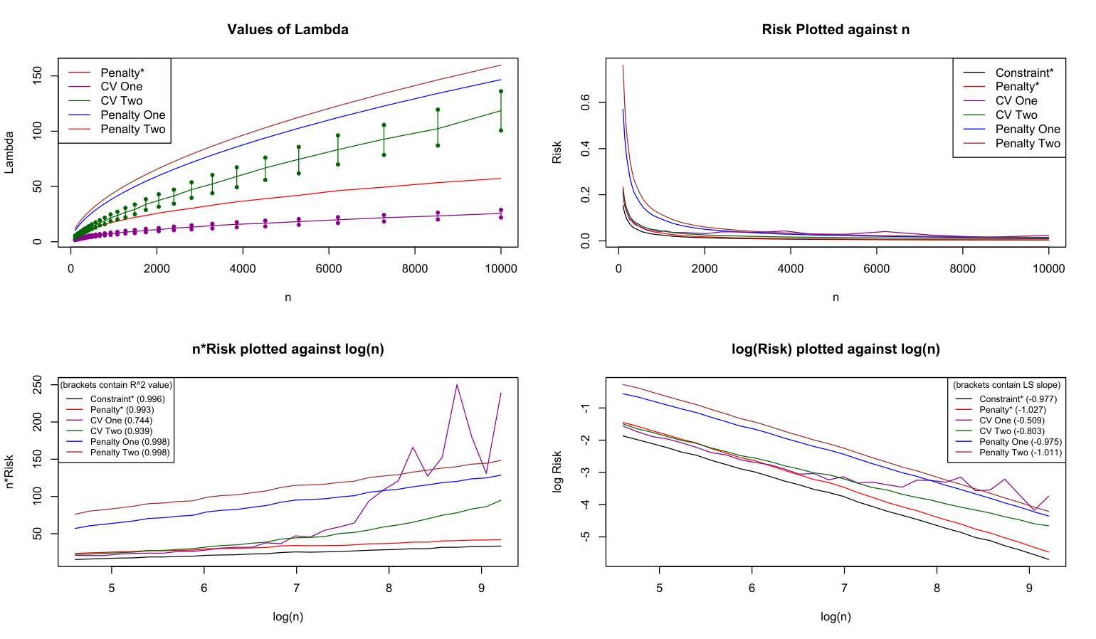
From f1∗f_{1}^{*} and a value of nn (chosen from a grid of size 30 between 100 and 10000; the grid being equally spaced on the logarithmic scale) we generated an n×1n\times 1 observation vector Y∼Nn​(θ∗,In)Y\sim N_{n}(\theta^{*},I_{n}) where θ∗\theta^{*} is the vector obtained by sampling f1∗f_{1}^{*} at nn equally spaced points with end-points 0 and 1. We then computed the following six estimators on the data vector YY: (a) the ideal constrained estimator (3) with V=V∗=‖D​θ∗‖1V=V^{*}=\|D\theta^{*}\|_{1}, (b) the ideal penalized estimator (4) with λ=λ∗\lambda=\lambda^{*} (as defined in (27)), (c) two cross-validation (CV) based estimators, (d) the penalized estimator (4) with λ\lambda of the form (39) with Γ=1\Gamma=1, and (e) the penalized estimator (4) with λ\lambda of the form (41) with Γ=0.5\Gamma=0.5. Corollary 2.10 proves that the risk with these λ\lambda choices decays as (log⁡n)/n(\log n)/n (ignoring terms involving kk) provided Γ\Gamma is taken to be a large enough constant. In our simulations for f1∗f_{1}^{*}, we found that Γ=1\Gamma=1 in (39) and Γ=0.5\Gamma=0.5 in (41) were large enough to yield the desired performance. Higher values of Γ\Gamma led to similar rates of decay of the risk with nn (even though the risk itself seemed to become larger with Γ\Gamma).

Here are some details behind the computation of these estimates. The constrained estimator was computed by the convex optimization software MOSEK (via the R package Rmosek). The penalized estimators were computed via the R package tvd for total variation denoising. The computation of the ideal penalized estimator requires computing the value of λ∗\lambda^{*} and, for this, we need to compute 𝔼​λθ∗​(Z){\mathbb{E}}\lambda_{\theta^{*}}(Z) (where Z∼Nn​(0,In)Z\sim N_{n}(0,I_{n})) and 2/‖v0‖2/\|v_{0}\| (see (27)). 2/‖v0‖2/\|v_{0}\| was calculated by the formula (29). For 𝔼​λθ∗​(Z){\mathbb{E}}\lambda_{\theta^{*}}(Z), we used the fact that λθ∗​(z)\lambda_{\theta^{*}}(z) can be calculated by convex optimization for each z∈ℝnz\in{\mathbb{R}}^{n} which implies that the expectation can be computed by Monte-Carlo averaging. More details behind this are provided in Section E. The CV estimators were calculated using the R package genlasso which provides two penalized estimates based on CV: one based on choosing λ\lambda so as to minimize the CV error (C​V1CV_{1}) and the other based on choosing λ\lambda via the one standard error rule (C​V2CV_{2}).

Refer to caption
Fig 4: Plots when the true function is f1∗f_{1}^{*}. The top-left plot shows the λ∗\lambda^{*} values, the CV λ\lambda values (median and the first and third quartiles over 200 replications) and the values corresponding to the explicit penalties (39) with Γ=1\Gamma=1 and (41) with Γ=0.5\Gamma=0.5. The other three figures show the behavior of the risk as a function of nn. In the last two plots, the legend shows the value of R2R^{2} and the slope respectively for the curves corresponding to each estimator.

For each data set, we computed the value of the loss ‖θ^−θ∗‖2/n\|\hat{\theta}-\theta^{*}\|^{2}/n for each of these six estimates. We generated 600 replications of the data for each value of nn to compute the average value of the loss which is an approximation of the risk of each estimator. Our results are provided in Figure 4. The top-left plot shows the different values of λ\lambda employed by the estimators based on (4). Here we plotted the λ∗\lambda^{*} values as well as those corresponding to (39) with Γ=1\Gamma=1 (penalty one) and (41) with Γ=0.5\Gamma=0.5 (penalty two). In addition, we also plotted here the penality levels chosen by the CV estimators. These are random so we plotted their median and quartile values over the 600 replications. The remaining three plots in Figure 4 show the risks of the six estimators. In the top-right plot, the risk is simply plotted as a function of nn (from our theoretical results, the risk is supposed to decay like the curve n↦(t1/n)​log⁡(t2​n)n\mapsto(t_{1}/n)\log(t_{2}n) for two constants t1t_{1} and t2t_{2}). In the bottom-left plot, we plotted nn times the risk against log⁡n\log n. These curves are supposed to be linear so we provided the squared correlation (R2R^{2}) values of each of the curves in this plot. One can see that the R2R^{2} values are close to one for every estimator except C​V1CV_{1}. Finally, in the bottom-right plot, we plotted the logarithm of the risk against log⁡n\log n. We expect the curves here to have a near-linear relationship with negative slope of −1-1. The least squares slope values for the different curves are given in the legend in this and it is clear that, for the non-CV estimators, the slope is indeed close to −1-1.

The numerical results in Figure 4 for the non-CV estimates therefore clearly support our theoretical results. On the other hand, the behavior of the CV estimators seems more complicated and a theoretical study of their risk performance is beyond the scope of the present paper.

We also show results for f2∗f_{2}^{*} where we evaluated the performance of trend filtering for r=2r=2. We did a simplified study here with the three estimators: (a) the ideal constrained estimator (3) with V=V∗=n​‖D2​θ∗‖1V=V^{*}=n\|D^{2}\theta^{*}\|_{1}, (b) the penalized estimator (4) with λ\lambda taken to be (50) with Γ=1/16\Gamma=1/16, and (c) the penalized estimator (4) with λ\lambda taken to be (52) with Γ=1/16\Gamma=1/16. Note that our theoretical results apply to (50) and (52) for a sufficiently large Γ\Gamma. For f2∗f_{2}^{*}, we found in simulations that Γ=1/16\Gamma=1/16 was large enough to yield the desired rates. Higher values of Γ\Gamma inflated risk but gave similar risk decay rates. We could not compute the ideal penalized estimator with λ=λ∗\lambda=\lambda^{*} (defined in (27)) here as the convex optimization problem to compute λθ∗​(z)\lambda_{\theta^{*}}(z) was highly ill-conditioned for n≥1000n\geq 1000 so that MOSEK seemed unable to find the global minimum (see Section E for more details). We also did not compute CV estimates here as these are not the focus of this paper.

Fig 5: Risk plots when the true function is f2∗f_{2}^{*}.

Our results are given in Figure 5. The left plot shows nn times the risk plotted against log⁡n\log n. Our theory indicates that the curve corresponding to each estimator should be linear so we provided the squared correlation (R2R^{2}) values which are all close to 1. The right plot shows the behavior of log risk against log⁡n\log n. These curves are expected to have a near-linear relationship with negative slope of −1-1. The legend shows the least squares slopes which are all close to −1-1. These plots therefore support our theoretical results.

5 Discussion

In this section, we address various issues that are naturally linked to our main results.

5.1 Weakening our assumptions

We emphasized the vector estimation setting (2) in this paper. Our results can also be interpreted in the function estimation setting in the following way. There is an unknown function f∗f^{*} and we observe data Y1,…,YnY_{1},\dots,Y_{n} according to the model:

Yi=f∗​(xi)+ξifor i=1,…,nY_{i}=f^{*}(x_{i})+\xi_{i}\qquad\text{for $i=1,\dots,n$}

where f∗:[0,1]→ℝf^{*}:[0,1]\rightarrow{\mathbb{R}} is the unknown regression function and ξ1,…,ξn\xi_{1},\dots,\xi_{n} are i.i.d. N⁡(0,σ2)N(0,\sigma^{2}). We focussed on the situation where xi=i/nx_{i}=i/n for i=1,…,ni=1,\dots,n. We can estimate f∗f^{*} by any discrete spline f^\hat{f} of degree r−1r-1 whose values at i/n,1=1,…,ni/n,1=1,\dots,n, are given by θ^1,…,θ^n\hat{\theta}_{1},\dots,\hat{\theta}_{n} (with θ^\hat{\theta} defined as in (3) or (4)). We then evaluate the performance of f^\hat{f} as an estimator for f∗f^{*} via the loss 1n​∑i=1n(f∗​(xi)−f^​(xi))2\frac{1}{n}\sum_{i=1}^{n}(f^{*}{(x_{i})}-\hat{f}(x_{i}))^{2} and prove bounds for the risk when f∗f^{*} is a discrete spline in terms of the number of polynomials that make up f∗f^{*}.

This basic setting (which is standard and used in many theoretical papers on univariate nonparametric regression) can be generalized in many ways and we mention two extensions involving the design points x1,…,xnx_{1},\dots,x_{n} below. One is the situation where x1,…,xnx_{1},\dots,x_{n} are not equally spaced. In this case, note that the penalty terms in (3) and (4) need to be changed for r≥2r\geq 2; see e.g., Tibshirani [46]. We believe that our results will still hold in this case provided x1,…,xnx_{1},\dots,x_{n} satisfy κ1/n≤xi−xi−1≤κ2/n\kappa_{1}/n\leq x_{i}-x_{i-1}\leq\kappa_{2}/n for two constants κ1\kappa_{1} and κ2\kappa_{2}. However, this would make the notation in our proofs quite cumbersome.

One can also study the setting where x1,…,xnx_{1},\dots,x_{n} are generated independently from a common distribution ν\nu on [0,1][0,1] and/or we measure the loss via ∫(f^​(x)−f∗​(x))2​𝑑ν​(x).\int\left(\hat{f}(x)-f^{*}(x)\right)^{2}d\nu(x). Analyzing this situation will require handling additional approximation error terms and we will leave it for future work.

5.2 Constrained and penalized estimators

As mentioned in the Introduction, we have studied both constrained and penalized versions of trend filtering while previous papers have focussed on the penalized estimator alone. When the noise level σ\sigma tends to zero, it can be proved that the constrained estimator with V=V∗:=V(r)​(θ∗)V=V^{*}:=V^{(r)}(\theta^{*}) is better than the penalized estimator for every choice of the tuning parameter λ\lambda. More precisely,

limσ↓01σ2​R​(θ^V∗(r),θ∗)<limσ↓01σ2​R​(θ^λ(r),θ∗)for every λ∈[0,∞).\lim_{\sigma\downarrow 0}\frac{1}{\sigma^{2}}R(\hat{\theta}^{(r)}_{V^{*}},\theta^{*})<\lim_{\sigma\downarrow 0}\frac{1}{\sigma^{2}}R(\hat{\theta}^{(r)}_{\lambda},\theta^{*})\qquad\text{for every $\lambda\in[0,\infty)$}. (55)

Here λ\lambda is even allowed to depend on θ∗\theta^{*} as long as it is non-random. Inequality (55) follows from the results of Oymak and Hassibi [35] as described below: Oymak and Hassibi [35, Theorem 2.1] implies

limσ↓01σ2​R​(θ^V∗(r),θ∗)=1n​𝔼​(infv∈cone⁡(∂g⁡(θ∗))‖Z−v‖2)\lim_{\sigma\downarrow 0}\frac{1}{\sigma^{2}}R(\hat{\theta}^{(r)}_{V^{*}},\theta^{*})=\frac{1}{n}{\mathbb{E}}\left(\inf_{v\in{\mathrm{cone}}(\partial g(\theta^{*}))}\|Z-v\|^{2}\right) (56)

and Oymak and Hassibi [35, Theorem 1.1] implies

limσ↓01σ2​R​(θ^λ(r),θ∗)=1n​𝔼​(infv∈λ​∂g⁡(θ∗)‖Z−v‖2)\lim_{\sigma\downarrow 0}\frac{1}{\sigma^{2}}R(\hat{\theta}^{(r)}_{\lambda},\theta^{*})=\frac{1}{n}{\mathbb{E}}\left(\inf_{v\in\lambda\partial g(\theta^{*})}\|Z-v\|^{2}\right) (57)

for every λ≥0\lambda\geq 0. Here g⁡(θ):=nr−1​‖D(r)​θ‖1g(\theta):=n^{r-1}\|D^{(r)}\theta\|_{1}, λ​∂g⁡(θ∗):={λ​v:v∈∂g⁡(θ∗)}\lambda\partial g(\theta^{*}):=\{\lambda v:v\in\partial g(\theta^{*})\}, cone(∂g(θ∗)):=∪λ≥0λ∂g(θ∗){\mathrm{cone}}(\partial g(\theta^{*})):=\cup_{\lambda\geq 0}\lambda\partial g(\theta^{*}) and Z∼Nn​(0,In)Z\sim N_{n}(0,I_{n}). As cone⁡(∂g⁡(θ∗)){\mathrm{cone}}(\partial g(\theta^{*})) is strictly larger than λ​g​(θ∗)\lambda g(\theta^{*}) for every fixed λ>0\lambda>0, the right hand side of (56) will be strictly smaller than the right hand side of (57) which proves (55).

The implication of this inequality is that there exist settings (where σ\sigma is small) where the constrained estimator with V=V∗V=V^{*} is better than every penalized estimator. Therefore it makes sense to study the constrained estimator in addition to the penalized estimator.

5.3 Results for data-dependent tuning parameters

From a practical point of view, a major limitation of the results of this paper is that they only hold for ideal or oracle choices of the tuning parameters. Indeed, our strong sparsity risk bounds for the constrained estimator require VV to be close to V∗:=V(r)​(θ∗)V^{*}:=V^{(r)}(\theta^{*}). On the other hand, our risk bounds for the penalized estimator require knowledge of the noise level σ\sigma (note that the tuning parameter in (4) involves σ\sigma) as well as certain aspects of θ∗\theta^{*}. For example, the choices (27), (39) and (50) depend on certain properties of the locations and signs of the knots of θ∗\theta^{*}. The choices (41) and (52) have lesser dependence on θ∗\theta^{*} but they still depend on the constants c1c_{1} and c2c_{2} from the condition (48).

We would like to note that this feature is also present in earlier papers on the trend filtering estimators. The strong sparsity risk results of Lin et al. [30] hold for the tuning choice (43) which depends on θ∗\theta^{*}. The results of Dalalyan, Hebiri and Lederer [8] and Ortelli and van de Geer [34] hold for the tuning choice (44) which does not depend on θ∗\theta^{*} but depends on the noise level σ\sigma and the probability level δ\delta (note that these results of [8, 34] give only high probability statements and not expectation (risk) bounds).

We would like to highlight the problem of proving risk bounds under strong sparsity for completely data-dependent choices of the tuning parameters as a major open problem. One can approach this problem via the constrained estimator which would require estimation of the variation functional V(r)​(θ∗)V^{(r)}(\theta^{*}). Alternatively, one can approach this problem via the penalized estimator which would require estimation of σ\sigma and λ∗\lambda^{*} (defined in (27)). It will be interesting to see if the risk of log⁡(e​n)/n\log(en)/n (up to multiplicative factors depending on kk) will be achieved for a completely data dependent method of tuning.

5.4 Connections to results for the LASSO

The trend filtering estimators are closely related to the LASSO estimator of Tibshirani [45]. Indeed, for r=1r=1, it is easy to see that the constrained estimator θ^V(1)\hat{\theta}^{(1)}_{V} is exactly equal to X​β^VX\hat{\beta}_{V} where XX is the n×nn\times n matrix whose (i,j)t​h(i,j)^{th} entry equals I{i≥j}I\{i\geq j\} and β^V:=argminθ∈ℝn{‖Y−X​β‖2:∑i=2n|βi|≤V}\hat{\beta}_{V}:=\mathop{\rm argmin}_{\theta\in{\mathbb{R}}^{n}}\left\{\|Y-X\beta\|^{2}:\sum_{i=2}^{n}|\beta_{i}|\leq V\right\}. Therefore our strong sparsity risk results for θ^V(1)\hat{\theta}_{V}^{(1)} can simply be seen as results for the LASSO estimator for this special design matrix XX. This connection to LASSO also holds for r≥2r\geq 2 (see Tibshirani [46]).

Based on this link to the LASSO, it might seem possible to believe that our results might be derivable from general theorems about the LASSO. However, existing strong sparsity risk bounds for the LASSO impose stringent conditions on the design matrix (such as the compatibility condition or the restricted eigenvalue condition) which do not hold for this particular design matrix XX (see Dalalyan, Hebiri and Lederer [8]). The relaxed compatibility condition of [8] does hold who use this condition to prove rates under strong sparsity but this argument is not strong enough to yield the k+1n​log⁡e​nk+1\frac{k+1}{n}\log\frac{en}{k+1} bound. More importantly, it is not clear if the relaxed compatibility condition of [8] or a modified version of it holds for r≥2r\geq 2.

5.5 Comparison to the L0L^{0} estimators

It is natural to compare the performance of the trend-filtering estimators to the estimators obtained by replacing the L1L^{1} norm in (3) by the L0L^{0} norm:

θ^k(r):=argminθ∈ℝn{12​‖Y−θ‖2:‖D(r)​θ‖0≤k}\hat{\theta}^{(r)}_{k}:=\mathop{\rm argmin}_{\theta\in{\mathbb{R}}^{n}}\left\{\frac{1}{2}\|Y-\theta\|^{2}:\|D^{(r)}\theta\|_{0}\leq k\right\} (58)

Under strong sparsity i.e., ‖D(r)​θ∗‖0≤k\|D^{(r)}\theta^{*}\|_{0}\leq k, it should be possible to prove that

R⁡(θ^k(r),θ∗)≤Cr​σ2​(k+1)n​log⁡e​nk+1.R(\hat{\theta}^{(r)}_{k},\theta^{*})\leq C_{r}\frac{\sigma^{2}(k+1)}{n}\log\frac{en}{k+1}. (59)

A proof of this result for r=1r=1 can be found in the recent paper Gao, Han and Zhang [15, Theorem 2.1]. We could not find an exact reference for r≥2r\geq 2 but we believe that (59) should be true based on the regression connection described in the previous subsection and existing results for L0L^{0}-penalized estimators in linear regression (see e.g., [38, Theorem 4]).

From a comparison of (59) with (18), it might seem that the constrained trend filtering estimator (with V=V∗V=V^{*}) has similar performance under strong sparsity as that of the L0L^{0} estimator. However, it must be kept in mind here that (18) requires the minimum length condition (13) while the bound (59) for the L0L^{0} estimator does not require any such minimum length condition. Without the minimum length condition, the L1L^{1} estimator performs much worse compared to the L0L^{0} estimator as proved in the recent paper Fan and Guan [12]. Note, however, that the minimum length condition is quite natural from the point of view of estimating piecewise polynomial functions.

From a computational viewpoint, (58) can be efficiently computed for r=1r=1 via dynamic programming (see e.g., Winkler and Liebscher [53]) but it is not clear how to compute it for r≥2r\geq 2. On the other hand, the trend filtering estimators are efficiently computable for every r≥2r\geq 2 via convex optimization (see e.g., Arnold and Tibshirani [2] and Kim et al. [25] for details).

5.6 Connection to shape constrained estimators

Shape constrained regression estimators are closely related to the trend filtering estimators. Indeed, if one takes the constrained trend filtering estimator (3) and replaces the L1L^{1} constraint by a nonnegativity constraint on D(r)​θD^{(r)}\theta, then we obtain shape constrained estimators. Specifically, consider

θ^shape(r):=argminθ∈ℝn{12​‖Y−θ‖2:D(r)​θ≥0}.\hat{\theta}^{(r)}_{\mathrm{shape}}:=\mathop{\rm argmin}_{\theta\in{\mathbb{R}}^{n}}\left\{\frac{1}{2}\|Y-\theta\|^{2}:D^{(r)}\theta\geq 0\right\}. (60)

Here D(r)​θ≥0D^{(r)}\theta\geq 0 means that each component of the vector D(r)​θD^{(r)}\theta is nonnegative. When r=1r=1, (60) coincides with the classical isotonic least squares estimator and when r=2r=2, (60) coincides with the convex least squares estimator (see Groeneboom and Jongbloed [19] for an introduction to shape constrained estimation). Like the trend filtering estimators, the shape constrained estimators enjoy the property that D(r)​θ^shape(r)D^{(r)}\hat{\theta}^{(r)}_{\mathrm{shape}} is sparse. However, unlike the trend filtering estimators, there is no tuning parameter in (60) (of course, (60) is only applicable in situations where θ∗\theta^{*} satisfies the constraint D(r)​θ∗≥0D^{(r)}\theta^{*}\geq 0 exactly or in some approximate sense).

The risk of (60) under the strong sparsity assumption (and the shape assumption D(r)​θ≥0D^{(r)}\theta\geq 0) has received much recent attention (see Guntuboyina and Sen [20] for a recent survey). In Bellec [3], it was proved that

R(θ^shape(r),θ∗)≤infθ:D(r)​θ≥0(1n∥θ∗−θ∥2+Crσ2​(k+1)nloge​nk+1).R(\hat{\theta}^{(r)}_{\mathrm{shape}},\theta^{*})\leq\inf_{\theta:D^{(r)}\theta\geq 0}\left(\frac{1}{n}\|\theta^{*}-\theta\|^{2}+C_{r}\frac{\sigma^{2}(k+1)}{n}\log\frac{en}{k+1}\right). (61)

where k:=𝐤r​(θ)=‖D(r)​θ‖0k:={\mathbf{k}_{r}}(\theta)=\|D^{(r)}\theta\|_{0}. This result is very similar to our risk bounds for the constrained trend filtering estimator with the important difference that no minimum length condition is required for (61). It is interesting to note that we use the above result in the proof of Theorem 2.2.

Acknowledgements

We thank Ryan Tibshirani for informing us about the reference, Steidl, Didas and Neumann [44], and for many other helpful comments. We are also extremely thankful to the Associate Editor and the anonymous referees for very detailed comments on an earlier version of the paper. Their feedback greatly improved the quality of the paper.

Supplementary Material (including proofs of main results)

Here we provide proofs of the results in the paper and some additional simulation results. The material is organized as follows. Section A contains a summary of various existing results from the literature on convex-constrained least squares estimators as well as convex analysis and geometry that are needed for our main proofs. Section B contains proofs of our main results in Section 2 of the main paper. Section C contains proofs of various technical supporting results that were crucially used in the proofs of Section B. Section D contains additional technical results and proofs. Finally Section E contains some additional simulation results.

A Preliminaries

In this section, we state some existing general results on the risk of constrained and penalized least squares estimators from the literature. These results will be used in the proofs of our main theorems from Section 2. We shall also state some standard results from convex analysis and convex geometry which will be used in our arguments.

Let us start with results for convex constrained least squares estimators. These are estimators of the form

θ^:=argminθ∈ℝn{12​‖Y−θ‖2:θ∈K}.\hat{\theta}:=\mathop{\rm argmin}_{\theta\in{\mathbb{R}}^{n}}\left\{\frac{1}{2}\|Y-\theta\|^{2}:\theta\in K\right\}. (62)

for a closed convex set KK. Note that the constrained trend filtering estimator θ^V(r)\hat{\theta}_{V}^{(r)} is a special case of this estimator when KK is taken to be the set K(r)​(V)K^{(r)}(V) defined as

K(r)​(V):={θ∈ℝn:‖D(r)​θ‖1≤V​n1−r}.K^{(r)}(V):=\left\{\theta\in{\mathbb{R}}^{n}:\|D^{(r)}\theta\|_{1}\leq Vn^{1-r}\right\}. (63)

The general theory of convex-constrained least squares estimators has a long history and is, by now, well established (see e.g., Van de Geer [47], Van der Vaart and Wellner [50], Hjort and Pollard [23], Chatterjee [7]). The following result, essentially from Chatterjee [7] (see Remark A.1) provides upper bounds for the risk of θ^\hat{\theta}. This result will be used in the proof of Theorem 2.1.

Theorem A.1.

Suppose Y∼Nn​(θ∗,σ2​In)Y\sim N_{n}(\theta^{*},\sigma^{2}I_{n}) for some θ∗∈K\theta^{*}\in K and consider the estimator (62). Then there exists a universal positive constant CC such that

R⁡(θ^,θ∗):=1n​𝔼θ∗​‖θ^−θ∗‖2≤Cn​max⁡(t02,σ2)R(\hat{\theta},\theta^{*}):=\frac{1}{n}{\mathbb{E}}_{\theta^{*}}\|\hat{\theta}-\theta^{*}\|^{2}\leq\frac{C}{n}\max(t_{0}^{2},\sigma^{2}) (64)

for every t0>0t_{0}>0 which satisfies

𝔼[supθ∈K:‖θ−θ∗‖≤t0⟨ξ,θ−θ∗⟩]≤t022where ξ∼Nn​(0,σ2​In).{\mathbb{E}}\left[\sup_{\theta\in K:\|\theta-\theta^{*}\|\leq t_{0}}\left<\xi,\theta-\theta^{*}\right>\right]\leq\frac{t_{0}^{2}}{2}\qquad\text{where $\xi\sim N_{n}(0,\sigma^{2}I_{n})$}. (65)
Remark A.1.

The purpose of this remark is to describe how Theorem A.1 follows from the results of Chatterjee [7] which are all stated for σ=1\sigma=1. Extending Chatterjee [7, Proof of Theorem 1.1] in a straightforward manner to the case of arbitrary σ>0\sigma>0, one obtains that

ℙ{∥θ^−θ∗∥−tθ∗≥xtθ∗}≤3exp(−x432​σ2​(1+x/tθ∗)2){\mathbb{P}}\left\{\|\hat{\theta}-\theta^{*}\|-t_{\theta^{*}}\geq x\sqrt{t_{\theta^{*}}}\right\}\leq 3\exp\left(\frac{-x^{4}}{32\sigma^{2}\left(1+x/\sqrt{t_{\theta^{*}}}\right)^{2}}\right) (66)

for every x≥0x\geq 0 where tθ∗t_{\theta^{*}} is defined as the maximizer of

t↦𝔼[supθ∈K:‖θ−θ∗‖≤t⟨ξ,θ−θ∗⟩]−t22t\mapsto{\mathbb{E}}\left[\sup_{\theta\in K:\|\theta-\theta^{*}\|\leq t}\left<\xi,\theta-\theta^{*}\right>\right]-\frac{t^{2}}{2}

over t≥0t\geq 0. Inequality (66) implies that whenever x≥tθ∗x\geq\sqrt{t_{\theta^{*}}}, we obtain

ℙ{∥θ^−θ∗∥−tθ∗≥xtθ∗}≤3exp(−tθ∗​x2128​σ2).{\mathbb{P}}\left\{\|\hat{\theta}-\theta^{*}\|-t_{\theta^{*}}\geq x\sqrt{t_{\theta^{*}}}\right\}\leq 3\exp\left(\frac{-t_{\theta^{*}}x^{2}}{128\sigma^{2}}\right).

This is because 1+x/tθ∗≤2​x/tθ∗1+x/\sqrt{t_{\theta^{*}}}\leq 2x/\sqrt{t_{\theta^{*}}} under the assumption that x≥tθ∗x\geq\sqrt{t_{\theta^{*}}}. Replacing xx by u/tθ∗u/\sqrt{t_{\theta^{*}}}, we obtain

ℙ{∥θ^−θ∗∥−tθ∗≥u}≤3exp(−u2128​σ2)for u≥tθ∗.{\mathbb{P}}\left\{\|\hat{\theta}-\theta^{*}\|-t_{\theta^{*}}\geq u\right\}\leq 3\exp\left(\frac{-u^{2}}{128\sigma^{2}}\right)\qquad\text{for $u\geq t_{\theta^{*}}$}.

Multiplying both sides by uu and integrating from u=tθ∗u=t_{\theta^{*}} to u=∞u=\infty, we get

𝔼​((‖θ^−θ∗‖−tθ∗)2−tθ∗2)+≤3​∫0∞u​exp⁡(−u2128​σ2)​𝑑u≤C​σ2.{\mathbb{E}}\left(\left(\|\hat{\theta}-\theta^{*}\|-t_{\theta^{*}}\right)^{2}-t^{2}_{\theta^{*}}\right)_{+}\leq 3\int_{0}^{\infty}u\exp\left(\frac{-u^{2}}{128\sigma^{2}}\right)du\leq C\sigma^{2}.

This implies that (via a2≤2​(a−b)+2+2​b2a^{2}\leq 2(a-b)_{+}^{2}+2b^{2})

𝔼​(‖θ^−θ∗‖−tθ∗)2≤C​σ2+2​tθ∗2.{\mathbb{E}}\left(\|\hat{\theta}-\theta^{*}\|-t_{\theta^{*}}\right)^{2}\leq C\sigma^{2}+2t_{\theta^{*}}^{2}.

which further implies that

𝔼​‖θ^−θ∗‖2≤6​tθ∗2+C​σ2≤C​max⁡(tθ∗2,σ2).{\mathbb{E}}\|\hat{\theta}-\theta^{*}\|^{2}\leq 6t_{\theta^{*}}^{2}+C\sigma^{2}\leq C\max\left(t_{\theta^{*}}^{2},\sigma^{2}\right).

From here, we obtain (64) by noting that tθ∗≤t0t_{\theta^{*}}\leq t_{0} which follows from Chatterjee [7, Proposition 1.3].

The risk of θ^\hat{\theta} can also be related to the tangent cones of the closed convex set KK at θ∗\theta^{*}. To describe these results, we need some notation and terminology. The tangent cone of KK at θ∈K\theta\in K is defined as

TK(θ):=Closure{t(η−θ):t≥0,η∈K}.T_{K}(\theta):=\mathrm{Closure}\{t(\eta-\theta):t\geq 0,\eta\in K\}. (67)

Informally, TK​(θ)T_{K}(\theta) represents all directions in which one can move from θ\theta and still remain in KK. Note that TK​(θ)T_{K}(\theta) is a cone which means that a​α∈TK​(θ)a\alpha\in T_{K}(\theta) for every α∈TK​(θ)\alpha\in T_{K}(\theta) and a≥0a\geq 0. It is also easy to see that TK​(θ)T_{K}(\theta) closed and convex.

The statistical dimension of a closed convex cone T⊆ℝnT\subseteq{\mathbb{R}}^{n} is defined as

δ⁡(T):=𝔼​‖ΠT​(Z)‖2where Z∼Nn​(0,In)\delta(T):={\mathbb{E}}\|\Pi_{T}(Z)\|^{2}\qquad\text{where $Z\sim N_{n}(0,I_{n})$}

and ΠT​(Z):=argminu∈T‖Z−u‖2\Pi_{T}(Z):=\mathop{\rm argmin}_{u\in T}\|Z-u\|^{2} is the projection of ZZ onto TT. The terminology of statistical dimension is due to Amelunxen et al. [1] and we refer the reader to this paper for many properties of the statistical dimension. The statistical dimension δ⁡(T)\delta(T) is closely related to the Gaussian width of TT which is defined as

w(T):=𝔼[supθ∈T:‖θ‖≤1⟨Z,θ⟩]where Z∼Nn​(0,In).w(T):={\mathbb{E}}\left[\sup_{\theta\in T:\|\theta\|\leq 1}\left<Z,\theta\right>\right]\qquad\text{where $Z\sim N_{n}(0,I_{n})$}. (68)

Indeed, it has been shown in Amelunxen et al. [1, Proposition 10.2] that

w2​(T)≤δ⁡(T)≤w2​(T)+1w^{2}(T)\leq\delta(T)\leq w^{2}(T)+1 (69)

for every closed convex cone TT.

The relevance of these notions to the estimator θ^\hat{\theta} (defined in (62)) is that the risk of θ^\hat{\theta} can be related to the statistical dimension of tangent cones of KK. This is the content of the following result due to Bellec [3, Corollary 2.2].

Theorem A.2.

Suppose Y∼Nn​(θ∗,σ2​In)Y\sim N_{n}(\theta^{*},\sigma^{2}I_{n}) for some θ∗∈ℝn\theta^{*}\in{\mathbb{R}}^{n}. Then

R⁡(θ^,θ∗)≤infθ∈K[1n​‖θ−θ∗‖2+σ2n​δ​(TK​(θ))].R(\hat{\theta},\theta^{*})\leq\inf_{\theta\in K}\left[\frac{1}{n}\|\theta-\theta^{*}\|^{2}+\frac{\sigma^{2}}{n}\delta(T_{K}(\theta))\right]. (70)

Moreover for every x>0x>0, we have

1n​‖θ^−θ∗‖2≤infθ∈K[1n​‖θ−θ∗‖2+2​σ2n​δ​(TK​(θ))]+4​σ2​xn\frac{1}{n}\|\hat{\theta}-\theta^{*}\|^{2}\leq\inf_{\theta\in K}\left[\frac{1}{n}\|\theta-\theta^{*}\|^{2}+\frac{2\sigma^{2}}{n}\delta(T_{K}(\theta))\right]+\frac{4\sigma^{2}x}{n}

with probability at least 1−e−x1-e^{-x}.

Remark A.2.

A useful lower bound corresponding to (70) has been proved by Oymak and Hassibi [35, Theorem 2.1]. This result states that when θ∗∈K\theta^{*}\in K, we have

limσ↓01σ2​R​(θ^,θ∗)=1n​δ​(TK​(θ∗))\lim_{\sigma\downarrow 0}\frac{1}{\sigma^{2}}R(\hat{\theta},\theta^{*})=\frac{1}{n}\delta(T_{K}(\theta^{*})) (71)

which means that δ⁡(TK​(θ∗))/n\delta(T_{K}(\theta^{*}))/n provides a precise description of R⁡(θ^,θ∗)R(\hat{\theta},\theta^{*}) in the low σ\sigma limit. The fact (71) will be used in the proof of Lemma 2.4.

An interesting aspect of Theorem A.2 is that θ∗\theta^{*} is allowed to be any vector in ℝn{\mathbb{R}}^{n}; in particular, it is not necessary that θ∗∈K\theta^{*}\in K. Note that combining Theorem A.2 with the bound δ⁡(T)≤w2​(T)+1\delta(T)\leq w^{2}(T)+1 from (69), we obtain the following risk and loss bounds in terms of the Gaussian width of tangent cones:

R⁡(θ^,θ∗)≤infθ∈K[1n​‖θ−θ∗‖2+σ2n+σ2n​w2​(TK​(θ))]R(\hat{\theta},\theta^{*})\leq\inf_{\theta\in K}\left[\frac{1}{n}\|\theta-\theta^{*}\|^{2}+\frac{\sigma^{2}}{n}+\frac{\sigma^{2}}{n}w^{2}(T_{K}(\theta))\right] (72)

and for every x>0x>0,

1n​‖θ^−θ∗‖2≤infθ∈K[1n​‖θ−θ∗‖2+2​σ2n+2​σ2n​w2​(TK​(θ))]+4​σ2​xn\frac{1}{n}\|\hat{\theta}-\theta^{*}\|^{2}\leq\inf_{\theta\in K}\left[\frac{1}{n}\|\theta-\theta^{*}\|^{2}+\frac{2\sigma^{2}}{n}+\frac{2\sigma^{2}}{n}w^{2}(T_{K}(\theta))\right]+\frac{4\sigma^{2}x}{n} (73)

with probability at least 1−e−x1-e^{-x}. The above pair of bounds will be our starting points in the proof of Theorem 2.2. With these bounds, the main task for proving Theorem 2.2 (as well as inequality (16) in Remark 2.3) will involve showing the existence of a constant CrC_{r} depending only on rr such that

w⁡(TK(r)​(V)​(θ))≤Cr​n​Δr​(θ)w(T_{K^{(r)}(V)}(\theta))\leq C_{r}\sqrt{n\Delta_{r}(\theta)} (74)

for every θ∈ℝn\theta\in{\mathbb{R}}^{n} with V(r)​(θ)=VV^{(r)}(\theta)=V. Indeed, combining the inequalities (72) and (74), we obtain

R⁡(θ^,θ∗)≤infθ∈K[1n​‖θ−θ∗‖2+σ2n+Cr2​σ2​Δr​(θ)].R(\hat{\theta},\theta^{*})\leq\inf_{\theta\in K}\left[\frac{1}{n}\|\theta-\theta^{*}\|^{2}+\frac{\sigma^{2}}{n}+C_{r}^{2}\sigma^{2}\Delta_{r}(\theta)\right].

Because Δr​(θ)≥(k+1)/n≥1/n\Delta_{r}(\theta)\geq(k+1)/n\geq 1/n, the above bound clearly implies (15). Similarly, (73), combined with (74), implies (16). The key therefore is to prove (74) which is accomplished in Subsection B.2.

Let us now describe results for penalized estimators of the form θ^λg\hat{\theta}_{\lambda}^{g} defined as

θ^λg:=argminθ∈ℝn(12​‖Y−θ‖2+σ​λ​g​(θ))\hat{\theta}_{\lambda}^{g}:=\mathop{\rm argmin}_{\theta\in{\mathbb{R}}^{n}}\left(\frac{1}{2}\|Y-\theta\|^{2}+\sigma\lambda g(\theta)\right) (75)

where g:ℝn→ℝg:{\mathbb{R}}^{n}\rightarrow{\mathbb{R}} is a convex function. The risk of θ^λg\hat{\theta}^{g}_{\lambda} under Y∼Nn​(θ∗,σ2​In)Y\sim N_{n}(\theta^{*},\sigma^{2}I_{n}) can be bounded by the Gaussian mean squared distance (defined next) of the set λ​∂g⁡(θ∗):={λ​v:v∈∂g⁡(θ∗)}\lambda\partial g(\theta^{*}):=\{\lambda v:v\in\partial g(\theta^{*})\} where ∂g⁡(θ∗)\partial g(\theta^{*}) is the subdifferential of gg at θ∗\theta^{*}. The Gaussian mean squared distance 𝐃⁡(𝒞){\mathbf{D}}({\mathcal{C}}) of a nonempty set 𝒞⊆ℝn{\mathcal{C}}\subseteq{\mathbb{R}}^{n} is defined as

𝐃(𝒞):=𝔼[dist2(Z,𝒞)]where dist⁡(Z,𝒞):=infx∈𝒞‖Z−x‖{\mathbf{D}}({\mathcal{C}}):={\mathbb{E}}\left[{\mathrm{dist}}^{2}(Z,{\mathcal{C}})\right]\qquad\text{where ${\mathrm{dist}}(Z,{\mathcal{C}}):=\inf_{x\in{\mathcal{C}}}\|Z-x\|$} (76)

and Z∼Nn​(0,In)Z\sim N_{n}(0,I_{n}). The following result, due to Oymak and Hassibi [35, Theorem 2.2] bounds the risk of θ^λg\hat{\theta}_{\lambda}^{g} in terms of 𝐃⁡(λ​∂g⁡(θ∗)){\mathbf{D}}(\lambda\partial g(\theta^{*})).

Theorem A.3.

Suppose Y∼Nn​(θ∗,σ2​In)Y\sim N_{n}(\theta^{*},\sigma^{2}I_{n}). Then

R⁡(θ^λg,θ∗)≤σ2n​𝐃​(λ​∂g⁡(θ∗)).R(\hat{\theta}_{\lambda}^{g},\theta^{*})\leq\frac{\sigma^{2}}{n}{\mathbf{D}}(\lambda\partial g(\theta^{*})).

Theorem A.3 will be our starting point for proving Theorem 2.6. Note that the penalized trend filtering estimator θ^λ(r)\hat{\theta}^{(r)}_{\lambda} is a special case of (75) with g⁡(θ):=nr−1​‖D(r)​θ‖1g(\theta):=n^{r-1}\|D^{(r)}\theta\|_{1} so that Theorem A.3 will imply that the risk of θ^λ(r)\hat{\theta}^{(r)}_{\lambda} will be bounded by (σ2/n)(\sigma^{2}/n) times 𝐃⁡(λ​nr−1​∂f⁡(θ∗)){\mathbf{D}}(\lambda n^{r-1}\partial f(\theta^{*})) where f⁡(θ):=‖D(r)​θ‖1f(\theta):=\|D^{(r)}\theta\|_{1}. The goal then becomes that of bounding 𝐃⁡(λ​nr−1​∂f⁡(θ∗)){\mathbf{D}}(\lambda n^{r-1}\partial f(\theta^{*})) from above in the case when D(r)​θ∗≠0D^{(r)}\theta^{*}\neq 0 (note that Theorem 2.6 does not deal with the case D(r)​θ∗=0D^{(r)}\theta^{*}=0; this case is dealt with in Lemma 2.14 whose proof is simpler and more direct).

Our idea for bounding 𝐃⁡(λ​nr−1​∂f⁡(θ∗)){\mathbf{D}}(\lambda n^{r-1}\partial f(\theta^{*})) is to relate it to the smaller quantity 𝐃⁡(cone⁡(∂f⁡(θ∗))){\mathbf{D}}({\mathrm{cone}}(\partial f(\theta^{*}))) where cone⁡(∂f⁡(θ∗)){\mathrm{cone}}(\partial f(\theta^{*})) is the convex cone generated by ∂f⁡(θ∗)\partial f(\theta^{*}):

cone(∂f(θ∗)):=∪λ≥0[λ∂f(θ∗)].{\mathrm{cone}}(\partial f(\theta^{*})):=\cup_{\lambda\geq 0}\left[\lambda\partial f(\theta^{*})\right].

It is clear that cone⁡(∂f⁡(θ∗)){\mathrm{cone}}(\partial f(\theta^{*})) contains the set λ​nr−1​∂f⁡(θ∗)\lambda n^{r-1}\partial f(\theta^{*}) for every λ≥0\lambda\geq 0 and thus by definition of 𝐃⁡(⋅){\mathbf{D}}(\cdot), it follows that

𝐃⁡(λ​nr−1​∂f⁡(θ∗))≥𝐃⁡(cone⁡(∂f⁡(θ∗))).{\mathbf{D}}(\lambda n^{r-1}\partial f(\theta^{*}))\geq{\mathbf{D}}({\mathrm{cone}}(\partial f(\theta^{*}))).

However, we need an upper bound and not a lower bound for 𝐃⁡(λ​nr−1​∂f⁡(θ∗)){\mathbf{D}}(\lambda n^{r-1}\partial f(\theta^{*})). It turns out that an upper bound can indeed be given for 𝐃⁡(λ​nr−1​∂f⁡(θ∗)){\mathbf{D}}(\lambda n^{r-1}\partial f(\theta^{*})) in terms of 𝐃⁡(cone⁡(∂f⁡(θ∗))){\mathbf{D}}({\mathrm{cone}}(\partial f(\theta^{*}))) and additional terms (involving λ\lambda and the vectors v0v_{0} and v∗v^{*} defined in (25)). This result (formally stated in Proposition B.5) can be seen as a generalization of Foygel and Mackey [13, Proposition 1]. The advantage of Proposition B.5 is that it reduces the task to upper bounding 𝐃⁡(cone⁡(∂f⁡(θ∗))){\mathbf{D}}({\mathrm{cone}}(\partial f(\theta^{*}))). As we shall outline below, by some standard facts from convex analysis, it follows that

𝐃⁡(cone⁡(∂f⁡(θ∗)))=δ⁡(TK(r)​(V∗)​(θ∗))≤1+w2​(TK(r)​(V∗)​(θ∗)){\mathbf{D}}({\mathrm{cone}}(\partial f(\theta^{*})))=\delta(T_{K^{(r)}(V^{*})}(\theta^{*}))\leq 1+w^{2}(T_{K^{(r)}(V^{*})}(\theta^{*})) (77)

where V∗:=V(r)​(θ∗)V^{*}:=V^{(r)}(\theta^{*}). This allows us to use the bound (74) (established in the course of the proof of Theorem 2.2) to bound 𝐃⁡(cone⁡(∂f⁡(θ∗))){\mathbf{D}}({\mathrm{cone}}(\partial f(\theta^{*}))).

We shall now explain why (77) is true. Note that we only need to prove the first equality (the second inequality is a consequence of (69)). For this, we need to introduce the notions of normal cone and polar cone from convex analysis (see, for example, Rockafellar [39] for background on these standard notions). The normal cone of a convex set 𝒞⊆ℝn{\mathcal{C}}\subseteq{\mathbb{R}}^{n} at a point x∈𝒞x\in{\mathcal{C}} is defined by

N𝒞​(x):={u∈ℝn:⟨y−x,u⟩≤0​ for every ​y∈𝒞}.N_{{\mathcal{C}}}(x):=\left\{u\in{\mathbb{R}}^{n}:\left<y-x,u\right>\leq 0\text{ for every }y\in{\mathcal{C}}\right\}.

Next let us define the notion of a polar cone. The polar ToT^{\mathrm{o}} of a nonempty closed convex cone T⊆ℝnT\subseteq{\mathbb{R}}^{n} is defined as

To:={u∈ℝn:⟨u,x⟩≤0 for every x∈T}.T^{\mathrm{o}}:=\left\{u\in{\mathbb{R}}^{n}:\left<u,x\right>\leq 0\text{ for every }x\in T\right\}. (78)

The following result (see, for example, Rockafellar and Wets [40, Example 6.24]) states that for every convex set 𝒞{\mathcal{C}} and x∈𝒞x\in{\mathcal{C}}, the normal cone N𝒞​(x)N_{{\mathcal{C}}}(x) equals the polar of the tangent cone T𝒞​(x)T_{{\mathcal{C}}}(x) (recall that T𝒞​(x)T_{{\mathcal{C}}}(x) is defined in (67)).

Lemma A.4.

For every convex set 𝒞⊆ℝn{\mathcal{C}}\subseteq{\mathbb{R}}^{n} and x∈𝒞x\in{\mathcal{C}}, we have

N𝒞​(x)=(T𝒞​(x))o.N_{{\mathcal{C}}}(x)=\left(T_{{\mathcal{C}}}(x)\right)^{\mathrm{o}}.

The next result states that cone⁡(∂f⁡(θ∗)){\mathrm{cone}}(\partial f(\theta^{*})) equals N𝒞​(θ∗)N_{{\mathcal{C}}}(\theta^{*}) where

𝒞:={θ∈ℝn:f⁡(θ)≤f⁡(θ∗)}{\mathcal{C}}:=\left\{\theta\in{\mathbb{R}}^{n}:f(\theta)\leq f(\theta^{*})\right\} (79)

under some conditions on the convex function ff and θ∗\theta^{*}. This result follows from Rockafellar [39, Theorem 23.7 and Corollary 23.7.1].

Lemma A.5.

Suppose f:ℝn→ℝf:{\mathbb{R}}^{n}\rightarrow{\mathbb{R}} is a convex function and θ∗∈ℝn\theta^{*}\in{\mathbb{R}}^{n} is such that ∂f⁡(θ∗)\partial f(\theta^{*}) is a compact convex set with 0∉∂f⁡(θ∗)0\notin\partial f(\theta^{*}). Then

cone⁡(∂f⁡(θ∗))=N𝒞​(θ∗){\mathrm{cone}}(\partial f(\theta^{*}))=N_{{\mathcal{C}}}(\theta^{*})

where 𝒞{\mathcal{C}} is given by (79).

Observe now that when f⁡(θ):=‖D(r)​θ‖1f(\theta):=\|D^{(r)}\theta\|_{1} and θ∗\theta^{*} is such that D(r)​θ∗≠0D^{(r)}\theta^{*}\neq 0, the conditions in Lemma A.5 hold as can be seen from the characterization of ∂f⁡(θ∗)\partial f(\theta^{*}) in Proposition 2.5. The assumption that 0∉∂f⁡(θ∗)0\notin\partial f(\theta^{*}) holds because for every v∈∂f⁡(θ∗)v\in\partial f(\theta^{*}), we must have

∑i=jn(r+i−j−1r−1)​vi=sgn⁡((D(r)​θ∗)j−r)\sum_{i=j}^{n}{r+i-j-1\choose r-1}v_{i}={\mathrm{sgn}}((D^{(r)}\theta^{*})_{j-r})

for every jj such that (D(r)​θ∗)j−r≠0(D^{(r)}\theta^{*})_{j-r}\neq 0 (there must exist at least one such jj because of the assumption that D(r)​θ∗≠0D^{(r)}\theta^{*}\neq 0).

Further, for f⁡(θ):=‖D(r)​θ‖1f(\theta):=\|D^{(r)}\theta\|_{1}, it is easy to see that the set 𝒞{\mathcal{C}} in (79) satisfies

𝒞={θ∈ℝn:‖D(r)​θ‖1≤‖D(r)​θ∗‖1}=K(r)​(V(r)​(θ∗))=K(r)​(V∗){\mathcal{C}}=\left\{\theta\in{\mathbb{R}}^{n}:\|D^{(r)}\theta\|_{1}\leq\|D^{(r)}\theta^{*}\|_{1}\right\}=K^{(r)}(V^{(r)}(\theta^{*}))=K^{(r)}(V^{*})

because V∗:=V(r)​(θ∗)V^{*}:=V^{(r)}(\theta^{*}) and K(r)​(V)K^{(r)}(V) is defined as in (63). Putting together the conclusions of Lemma A.4 and Lemma A.5, we therefore deduce that

cone⁡(∂f⁡(θ∗))=(TK(r)​(V∗)​(θ∗))o.{\mathrm{cone}}(\partial f(\theta^{*}))=\left(T_{K^{(r)}(V^{*})}(\theta^{*})\right)^{\mathrm{o}}.

From here, in order to prove (77), we need another standard fact from convex geometry (see, for example, Hiriart-Urruty and Lemaréchal [22, Theorem 3.2.5]). This result states that for every closed convex cone T⊆ℝnT\subseteq{\mathbb{R}}^{n}, we have

ΠTo​(z)=z−ΠT​(z)for every z∈ℝn\Pi_{T^{\mathrm{o}}}(z)=z-\Pi_{T}(z)\qquad\text{for every $z\in{\mathbb{R}}^{n}$} (80)

where ΠK​(z)\Pi_{K}(z) denotes the projection of zz onto KK.

Applying (80) to T:=cone⁡(∂f⁡(θ∗))T:={\mathrm{cone}}(\partial f(\theta^{*})) (which is a closed convex cone when D(r)​θ∗≠0D^{(r)}\theta^{*}\neq 0; closedness follows, for example, from Rockafellar [39, Corollary 9.6.1]), we obtain

z−Πcone⁡(∂f⁡(θ∗))​(z)=ΠTK(r)​(V∗)​(z).z-\Pi_{{\mathrm{cone}}(\partial f(\theta^{*}))}(z)=\Pi_{T_{K^{(r)}(V^{*})}}(z). (81)

From the above identity (and the definitions of 𝐃⁡(⋅){\mathbf{D}}(\cdot) and δ⁡(⋅)\delta(\cdot)), the fact (77) readily follows. The fact (77) will be crucially used in the proof of Theorem 2.6. Also, the identity (81) will play a key role in the proofs of Lemma 2.9 and Lemma 2.12.

B Proofs of the Main Results

In the section, we provide the proofs of the following results in Section 2: Theorem 2.1, Theorem 2.2 (and inequality (16) in Remark 2.3), Corollary 2.3, Lemma 2.4, Theorem 2.6, Corollary 2.8, Lemma 2.9 and Corollary 2.10, Corollary 2.11, Lemma 2.12 and Corollary 2.13 and finally, Lemma 2.14. In addition to these results, Section 2 also contains Proposition 2.5 and Lemma 2.7. These are proved in Subsection C.4.

Some of the proofs presented in this section will introduce and use additional technical results. These technical results will be proved in the Section C.

B.1 Proof of Theorem 2.1

We prove Theorem 2.1 in this subsection. As mentioned at the start of Section A, our starting point for this proof is Theorem A.1; note that θ^V(r)\hat{\theta}^{(r)}_{V} is the least squares estimator subject to the constraint that θ∈K(r)​(V)\theta\in K^{(r)}(V) (recall that the set K(r)​(V)K^{(r)}(V) is defined in (63)). Theorem A.1 implies that we can bound the risk of θ^V(r)\hat{\theta}_{V}^{(r)} via upper bounds for

G(t):=𝔼[supθ∈K(r)​(V):‖θ−θ∗‖≤t⟨ξ,θ−θ∗⟩]G(t):={\mathbb{E}}\left[\sup_{\theta\in K^{(r)}(V):\|\theta-\theta^{*}\|\leq t}\left<\xi,\theta-\theta^{*}\right>\right] (82)

for t>0t>0. Our upper bound for G⁡(t)G(t) is proved from the following lemma. Let

Sr(V,t):={α∈ℝn:∥α∥≤t,∥D(r)α∥1≤Vn1−r}.S_{r}(V,t):=\left\{\alpha\in{\mathbb{R}}^{n}:\|\alpha\|\leq t,\|D^{(r)}\alpha\|_{1}\leq Vn^{1-r}\right\}. (83)
Lemma B.1.

Fix an integer r≥1r\geq 1. Then there exists a positive constant CrC_{r} such that for every n≥rn\geq r, t≥0t\geq 0 and V≥0V\geq 0, we have

𝔼⁡[supθ∈Sr​(V,t)⟨ξ,θ⟩]≤Cr​σ​t​(n​Vt)1/(2​r)+Cr​σ​t​log⁡(e​n).{\mathbb{E}}\left[\sup_{\theta\in S_{r}(V,t)}\left<\xi,\theta\right>\right]\leq C_{r}\sigma t\left(\frac{\sqrt{n}V}{t}\right)^{1/(2r)}+C_{r}\sigma t\sqrt{\log(en)}. (84)

Lemma B.1 is proved in Subsection C.3 and the ideas behind its proof are as follows. By Dudley’s entropy bound, the left hand side of (84) can be bounded from above by the metric entropy numbers (formally defined in Subsection C.3) of the set Sr​(V,t)S_{r}(V,t) (defined in (83)). The metric entropy of Sr​(V,t)S_{r}(V,t) will be bounded by controlling the fat shattering dimension (see Subsection C.1 for details).

Below, we provide the proof of Theorem 2.1 based on Lemma B.1.

Proof of Theorem 2.1.

As ‖D(r)​θ∗‖1≤V​n1−r\|D^{(r)}\theta^{*}\|_{1}\leq Vn^{1-r}, it follows that θ∗∈K(r)​(V)\theta^{*}\in{K^{(r)}(V)} (the set K(r)​(V){K^{(r)}(V)} is defined in (63)). Theorem A.1 implies that

R⁡(θ^V(r),θ∗)≤Cn​max⁡(t02,σ2)R(\hat{\theta}^{(r)}_{V},\theta^{*})\leq\frac{C}{n}\max\left(t_{0}^{2},\sigma^{2}\right) (85)

for a universal positive constant CC, where t0>0t_{0}>0 is such that G⁡(t0)≤t02/2G(t_{0})\leq t_{0}^{2}/2 with G⁡(t)G(t) defined as in (82). In order to apply this result, we need to bound the function G⁡(t)G(t) from above. By triangle inequality, ‖D(r)​(θ−θ∗)‖1≤‖D(r)​θ‖1+‖D(r)​θ∗‖1\|D^{(r)}(\theta-\theta^{*})\|_{1}\leq\|D^{(r)}\theta\|_{1}+\|D^{(r)}\theta^{*}\|_{1} so that

G(t)=𝔼supθ∈K(r)​(V):‖θ−θ∗‖≤t⟨ξ,θ−θ∗⟩≤𝔼supα∈ℝn:‖α‖≤t,‖D(r)​α‖1≤2​V​n1−r⟨ξ,α⟩.G(t)={\mathbb{E}}\sup_{\theta\in{K^{(r)}(V)}:\|\theta-\theta^{*}\|\leq t}\left<\xi,\theta-\theta^{*}\right>\leq{\mathbb{E}}\sup_{\alpha\in{\mathbb{R}}^{n}:\|\alpha\|\leq t,\|D^{(r)}\alpha\|_{1}\leq 2Vn^{1-r}}\left<\xi,\alpha\right>.

The right hand side above is controlled in Lemma B.1 from which we deduce that

G⁡(t)≤Cr​σ​t​(n​Vt)12​r+Cr​σ​t​log⁡(e​n)G(t)\leq C_{r}\sigma t\left(\frac{\sqrt{n}V}{t}\right)^{\frac{1}{2r}}+C_{r}\sigma t\sqrt{\log(en)}

for a constant CrC_{r} depending on rr alone. We now observe that

Cr​σ​t​(n​Vt)12​r≤t24​ iff ​t≥(4​Cr)2​r/(2​r+1)​σ2​r/(2​r+1)​(V​n)1/(2​r+1)C_{r}\sigma t\left(\frac{\sqrt{n}V}{t}\right)^{\frac{1}{2r}}\leq\frac{t^{2}}{4}~~\text{ iff }~~t\geq(4C_{r})^{2r/(2r+1)}\sigma^{2r/(2r+1)}\left(V\sqrt{n}\right)^{1/(2r+1)}

and

Cr​σ​t​log⁡(e​n)≤t24​ iff ​t≥4​Cr​σ​log⁡(e​n).C_{r}\sigma t\sqrt{\log(en)}\leq\frac{t^{2}}{4}~~\text{ iff }~~t\geq 4C_{r}\sigma\sqrt{\log(en)}.

It follows therefore that G⁡(t0)≤t02/2G(t_{0})\leq t_{0}^{2}/2 provided

t0:=max⁡((4​Cr)2​r/(2​r+1)​σ2​r/(2​r+1)​(V​n)1/(2​r+1),4​Cr​σ​log⁡(e​n)).t_{0}:=\max\left((4C_{r})^{2r/(2r+1)}\sigma^{2r/(2r+1)}\left(V\sqrt{n}\right)^{1/(2r+1)},4C_{r}\sigma\sqrt{\log(en)}\right).

The proof of inequality (8) is therefore complete by inequality (85).

Inequality (9) can be derived as a consequence of (8) and the fact that the map y↦‖θ^V(r)−θ∗‖y\mapsto\|\hat{\theta}^{(r)}_{V}-\theta^{*}\| is 1-Lipschitz (see e.g., van de Geer and Wainwright [49, Section 2]). By the usual concentration inequality for Lipschitz functions of Gaussian variables, this gives

ℙ{∥θ^V(r)−θ∗∥≥𝔼θ∗∥θ^V(r)−θ∗∥+σz}≤exp(−z22).{\mathbb{P}}\left\{\|\hat{\theta}^{(r)}_{V}-\theta^{*}\|\geq{\mathbb{E}}_{\theta^{*}}\|\hat{\theta}^{(r)}_{V}-\theta^{*}\|+\sigma z\right\}\leq\exp\left(\frac{-z^{2}}{2}\right).

This gives that

1n​‖θ^V(r)−θ∗‖2≤2​R​(θ^V(r),θ∗)+4​σ2​xn\frac{1}{n}\|\hat{\theta}^{(r)}_{V}-\theta^{*}\|^{2}\leq 2R(\hat{\theta}^{(r)}_{V},\theta^{*})+\frac{4\sigma^{2}x}{n}

with probability at least 1−e−x1-e^{-x} so that inequality (9) follows from (8). ∎

B.2 Proof of Theorem 2.2

Our starting points for proving Theorem 2.2 are the inequalities (72) and (73) applied to K=K(r)​(V)K=K^{(r)}(V). From here, it is clear that inequality (15) (as well as (16)) both follow from the inequality (74). Writing explicitly the Gaussian width w​(TK(r)​(V)​(θ))w(T_{K^{(r)}(V)}(\theta)), we see that (74) is equivalent to proving that

𝔼[supα∈TK(r)​(V)​(θ):‖α‖≤1⟨Z,α⟩]≤Crn​Δr​(θ){\mathbb{E}}\left[\sup_{\alpha\in T_{{K^{(r)}(V)}}(\theta):\|\alpha\|\leq 1}\left<Z,\alpha\right>\right]\leq C_{r}\sqrt{n\Delta_{r}(\theta)} (86)

for every θ∈ℝn\theta\in{\mathbb{R}}^{n} with V(r)​(θ)=VV^{(r)}(\theta)=V. For this, we obviously need to understand the set TK(r)​(V)​(θ)T_{{K^{(r)}(V)}}(\theta) for θ∈ℝn\theta\in{\mathbb{R}}^{n} with V(r)​(θ)=VV^{(r)}(\theta)=V. The following result provides a necessary condition that is satisfied by every vector α∈TK(r)​(V)​(θ)\alpha\in T_{{K^{(r)}(V)}}(\theta) with ‖α‖≤1\|\alpha\|\leq 1. The proof of this lemma is given in Subsection C.2. Recall, from Section 2, the notion of rt​hr^{th} order knots (along with their signs) of vectors in ℝn{\mathbb{R}}^{n}. We shall also use the following notation. For α∈ℝm\alpha\in{\mathbb{R}}^{m} and 1≤a≤b≤m1\leq a\leq b\leq m, we let

Va,b​(α):=V⁡(αa,…,αb)=|αa+1−αa|+⋯+|αb−αb−1|.V_{a,b}(\alpha):=V(\alpha_{a},\dots,\alpha_{b})=|\alpha_{a+1}-\alpha_{a}|+\dots+|\alpha_{b}-\alpha_{b-1}|. (87)
Lemma B.2.

Fix V>0V>0, r≥1r\geq 1, n≥rn\geq r and θ∈ℝn\theta\in{\mathbb{R}}^{n} with V(r)​(θ)=VV^{(r)}(\theta)=V. Suppose 2≤j1<⋯<jk≤n−r+12\leq j_{1}<\dots<j_{k}\leq n-r+1 denote any set of indices which contains all the rt​hr^{th} order knots of θ\theta. Let 𝔯1,…,𝔯k{\mathfrak{r}}_{1},\dots,{\mathfrak{r}}_{k} be such that 𝔯i{\mathfrak{r}}_{i} is the sign of the knot corresponding to jij_{i} if jij_{i} is a knot and 𝔯i{\mathfrak{r}}_{i} is arbitrary in {−1,0,1}\{-1,0,1\} if jij_{i} is not a knot. Also let j0=1j_{0}=1, jk+1=n−r+2j_{k+1}=n-r+2 and 𝔯0=𝔯k+1=0{\mathfrak{r}}_{0}={\mathfrak{r}}_{k+1}=0. The indices j0,j1,…,jk,jk+1j_{0},j_{1},\dots,j_{k},j_{k+1} define a partition ℐ0,…,ℐk{\mathcal{I}}_{0},\dots,{\mathcal{I}}_{k} of {1,…,n}\{1,\dots,n\} in the following way: ℐ0:={j0,…,j1+r−2}{\mathcal{I}}_{0}:=\{j_{0},\dots,j_{1}+r-2\} and

ℐi={ji+r−1,…,ji+1+r−2}for i=1,…,k.{\mathcal{I}}_{i}=\{j_{i}+r-1,\dots,j_{i+1}+r-2\}\qquad\text{for $i=1,\dots,k$}.

Let nin_{i} denote the cardinality of ℐi{\mathcal{I}}_{i} for i=0,1,…,ki=0,1,\dots,k i.e., n0:=j1+r−2n_{0}:=j_{1}+r-2 and ni=ji+1−jin_{i}=j_{i+1}-j_{i} for 1≤i≤k1\leq i\leq k. Then there exists a positive constant CrC_{r} (that depends on rr alone) such that for every α∈TK(r)​(V)​(θ)\alpha\in T_{{K^{(r)}(V)}}(\theta) with ‖α‖≤1\|\alpha\|\leq 1, there exist indices ℓ0∈ℐ0,ℓ1∈ℐ1,…,ℓk∈ℐk\ell_{0}\in{\mathcal{I}}_{0},\ell_{1}\in{\mathcal{I}}_{1},\dots,\ell_{k}\in{\mathcal{I}}_{k} such that

∑i=0kΓi​(α,ℓi)≤Cr​∑i=0kni1−2​rI{𝔯i≠𝔯i+1}\sum_{i=0}^{k}\Gamma_{i}(\alpha,\ell_{i})\leq C_{r}\sqrt{\sum_{i=0}^{k}n_{i}^{1-2r}I\{{\mathfrak{r}}_{i}\neq{\mathfrak{r}}_{i+1}\}} (88)

where

Γi​(α,ℓi):=Vji,ji+1−1​(Δ)−𝔯i+1​(Δji+1−1−Δℓi)−𝔯i​(Δℓi−Δji)\Gamma_{i}(\alpha,\ell_{i}):=V_{j_{i},j_{i+1}-1}(\Delta)-{\mathfrak{r}}_{i+1}(\Delta_{j_{i+1}-1}-\Delta_{\ell_{i}})-{\mathfrak{r}}_{i}(\Delta_{\ell_{i}}-\Delta_{j_{i}}) (89)

with Δ=(Δ1,…,Δn−r+1):=D(r−1)​α\Delta=(\Delta_{1},\ldots,\Delta_{n-r+1}):=D^{(r-1)}\alpha.

Remark B.1.

It may be noted that the indices j1,…,jkj_{1},\dots,j_{k} in Lemma B.2 are not exactly the knots of θ\theta. They are any set of indices that contain the knots of θ\theta. We shall mostly work with the case when j1,…,jkj_{1},\dots,j_{k} are exactly the set of knots of θ\theta but we shall need this additional generality to deal with one special situation when some of the distances between the knots of θ\theta are too large. In this case (see the last part of the proof of Theorem 2.2), we shall add additional indices to the knots in order to keep the inter-distances manageable.

The insight provided by Lemma B.2 into the structure of {α∈TK(r)​(V)​(θ):‖α‖≤1}\{\alpha\in T_{{K^{(r)}(V)}}(\theta):\|\alpha\|\leq 1\} (note that understanding this set is necessary for proving (86)) is as follows. Suppose that n0,…,nkn_{0},\dots,n_{k} are such that the right hand side of (88) is small. In this case, Lemma B.2 implies that for every α∈TK(r)​(V)​(θ)\alpha\in T_{{K^{(r)}(V)}}(\theta) with ‖α‖≤1\|\alpha\|\leq 1, there exist indices ℓ0,…,ℓk\ell_{0},\dots,\ell_{k} for which ∑i=0kΓi​(α,ℓi)\sum_{i=0}^{k}\Gamma_{i}(\alpha,\ell_{i}) is small. Figure 6 displays two unit norm vectors in the tangent cone of a piecewise constant vector θ\theta (i.e., r=1r=1) and the corresponding indices ℓ0,…,ℓk\ell_{0},\dots,\ell_{k}.

Fig 6: Let r=1r=1, n=200n=200 and let θ\theta be the vector obtained by sampling f1∗f_{1}^{*} at nn equally spaced points with end points 0 and 1 (here f1∗f_{1}^{*} is the piecewise constant vector from Section 4 of the main paper). This vector θ\theta has k=4k=4 jumps at j1=41,j2=81,j3=121j_{1}=41,j_{2}=81,j_{3}=121 and j4=161j_{4}=161. These indices (and the indices ji−1,i=1,2,3,4j_{i}-1,i=1,2,3,4) are plotted in black lines in the above pair of plots along with vertical straight lines at j0=1j_{0}=1 and j5=200j_{5}=200. We then considered the tangent cone, T:=TK(1)​(V)​(θ)T:=T_{K^{(1)}(V)}(\theta), where VV is the variation of θ\theta and plotted two vectors α\alpha in TT with ‖α‖=1\|\alpha\|=1. For each of these two vectors α\alpha, we also plotted the integers ℓ0,…,ℓ4\ell_{0},\dots,\ell_{4} as blue vertical lines. Informally, in the five constant segments corresponding to θ\theta, each vector α\alpha is approximately made of two monotone segments.

It is helpful here to observe that Γi​(α,ℓi)\Gamma_{i}(\alpha,\ell_{i}) is always nonnegative. Also, if Γi​(α,ℓi)=0\Gamma_{i}(\alpha,\ell_{i})=0, then D(r−1)​αD^{(r-1)}\alpha is made of two monotone pieces in the interval from jij_{i} to ji+1−1j_{i+1}-1 (one piece from jij_{i} to ℓi\ell_{i} and the other from ℓi\ell_{i} to ji+1−1j_{i+1}-1). When r=1r=1, this means that α\alpha is made of two monotone pieces in the interval from jij_{i} to ji+1−1j_{i+1}-1. When r=2r=2, this means that α\alpha is made of two convex/concave pieces in the interval from jij_{i} to ji+1−1j_{i+1}-1. For general rr, this means that α\alpha is made of two (r−1)t​h(r-1)^{th} order convex/concave functions in the interval from jij_{i} to ji+1−1j_{i+1}-1. Extending this argument, when Γi​(α,ℓi)\Gamma_{i}(\alpha,\ell_{i}) is small, D(r−1)​αD^{(r-1)}\alpha is nearly made of two monotone pieces in the interval from jij_{i} to ji+1−1j_{i+1}-1; equivalently α\alpha is nearly made of two (r−1)t​h(r-1)^{th} order convex/concave sequences in the interval from jij_{i} to ji+1−1j_{i+1}-1. This suggests therefore that in order to prove (86), we need to prove bounds on the Gaussian suprema for vectors α∈ℝn\alpha\in{\mathbb{R}}^{n} for which D(r−1)​αD^{(r-1)}\alpha is nearly monotone. This is the content of the next lemma which is another main ingredient for the proof of Theorem 2.2.

Lemma B.3.

Fix r≥1r\geq 1, n≥rn\geq r, 1≤l≤n−r+11\leq l\leq n-r+1, t>0t>0 and δ≥0\delta\geq 0. For θ∈ℝn\theta\in{\mathbb{R}}^{n}, let Δ⁡(θ)=(Δ1​(θ),…,Δn−r+1​(θ)):=D(r−1)​θ\Delta(\theta)=(\Delta_{1}(\theta),\ldots,\Delta_{n-r+1}(\theta)):=D^{(r-1)}\theta. Also let ξ∼Nn​(0,σ2​In)\xi\sim N_{n}(0,\sigma^{2}I_{n}). For every 𝔯1,𝔯2∈{−1,0,1}{\mathfrak{r}}_{1},{\mathfrak{r}}_{2}\in\{-1,0,1\}, the quantity

𝔼supθ∈ℝn,‖θ‖≤t{⟨ξ,θ⟩:Δ=Δ(θ),V(Δ)≤𝔯1(Δℓ−Δ1)+𝔯2(Δn−r+1−Δℓ)+δ}{\mathbb{E}}\sup_{\theta\in{\mathbb{R}}^{n},\|\theta\|\leq t}\left\{\left<\xi,\theta\right>:\Delta=\Delta(\theta),V(\Delta)\leq{\mathfrak{r}}_{1}(\Delta_{\ell}-\Delta_{1})+{\mathfrak{r}}_{2}(\Delta_{n-r+1}-\Delta_{\ell})+\delta\right\}

is bounded from above as

G≤Cr​σ​(t+δ​n(2​r−1)/2)​log⁡(e​n)+Cr​σ​t(2​r−1)/(2​r)​n(2​r−1)/(4​r)​δ1/(2​r)G\leq C_{r}\sigma\left(t+\delta n^{(2r-1)/2}\right)\sqrt{\log(en)}+C_{r}\sigma t^{(2r-1)/(2r)}n^{(2r-1)/(4r)}\delta^{1/(2r)}

for a positive constant CrC_{r} that depends on rr alone.

The proof of Lemma B.3 is given in Subsection C.3 (in fact, in Subsection C.3, we prove Lemma C.7 which is a more accurate result compared to Lemma B.3 in the sense that Lemma C.7 gives a bound that depends on the actual values of 𝔯1{\mathfrak{r}}_{1} and 𝔯2{\mathfrak{r}}_{2}). The proof of Lemma C.7 uses results on expected Gaussian suprema for classes of shape-constrained vectors from Bellec [3].

We are now ready to prove Theorem 2.2.

Proof of Theorem 2.2.

As the proof is rather long, we divide it into many steps.

Step I: We first note that the case when V=0V=0 is trivial. This is because the set {θ∈ℝn:‖D(r)​θ‖1=0}\{\theta\in{\mathbb{R}}^{n}:\|D^{(r)}\theta\|_{1}=0\} is a subspace of dimension rr so that θ^V=0(r)\hat{\theta}^{(r)}_{V=0} becomes a linear projection onto a subspace. Thus,

1n∥θ^(r)V=0−θ∗∥2−infθ∈ℝn:‖D(r)​θ‖1=01n∥θ−θ∗∥2∼σ2nχ2r\frac{1}{n}\|\hat{\theta}^{(r)}_{V=0}-\theta^{*}\|^{2}-\inf_{\theta\in{\mathbb{R}}^{n}:\|D^{(r)}\theta\|_{1}=0}\frac{1}{n}\|\theta-\theta^{*}\|^{2}\sim\frac{\sigma^{2}}{n}\chi^{2}_{r}

where χr2\chi^{2}_{r} denotes the chi-squared distribution with rr degrees of freedom. This and a standard tail bound for chi-squared random variables such as (see e.g., Laurent and Massart [27, Subsection 4.1])

ℙ{χr2≤2r+3x}≥1−e−xfor every x>0{\mathbb{P}}\left\{\chi^{2}_{r}\leq 2r+3x\right\}\geq 1-e^{-x}\qquad\text{for every $x>0$}

prove inequalities (15) and (16) for V=0V=0; note that when θ∈ℝn\theta\in{\mathbb{R}}^{n} is such that V(r)​(θ)=V=0V^{(r)}(\theta)=V=0, we have 𝐤r​(θ)=0{\mathbf{k}_{r}}(\theta)=0, δr​(θ)=n(1/2)−r\delta_{r}(\theta)=n^{(1/2)-r} and Δr​(θ)=2n​log⁡(e​n)+1n\Delta_{r}(\theta)=\frac{2}{n}\log(en)+\frac{1}{n}.

We shall assume from now on that V>0V>0. Based on the discussion at the beginning of this subsection, it is enough to prove (86). We therefore fix θ∈ℝn\theta\in{\mathbb{R}}^{n} with V(r)​(θ)=VV^{(r)}(\theta)=V. We need to bound the quantity

G:=𝔼[supα∈TK(r)​(V)​(θ):‖α‖≤1⟨Z,α⟩]G:={\mathbb{E}}\left[\sup_{\alpha\in T_{{K^{(r)}(V)}}(\theta):\|\alpha\|\leq 1}\left<Z,\alpha\right>\right] (90)

where ZZ is a standard nn-dimensional Gaussian random vector. We bound GG by breaking the set {α∈TK(r)​(V)​(θ):‖α‖≤1}\{\alpha\in T_{{K^{(r)}(V)}}(\theta):\|\alpha\|\leq 1\} into smaller subsets.

Let 2≤j1<⋯<jk≤n−r+12\leq j_{1}<\dots<j_{k}\leq n-r+1 denote all the rt​hr^{th} order knots of θ\theta. Also let 𝔯1,…,𝔯k∈{−1,1}{\mathfrak{r}}_{1},\dots,{\mathfrak{r}}_{k}\in\{-1,1\} denote the signs of the knots. For convenience, we take j0=1,jk+1=n−r+2j_{0}=1,j_{k+1}=n-r+2 and 𝔯0=𝔯k+1=0{\mathfrak{r}}_{0}={\mathfrak{r}}_{k+1}=0. Let n0=j1+r−2n_{0}=j_{1}+r-2 and nu=ju+1−jun_{u}=j_{u+1}-j_{u} for u=1,…,ku=1,\dots,k. Check that ∑u=0knu=n\sum_{u=0}^{k}n_{u}=n.

Step II: We shall prove (86) first under the simplifying assumption that

ni≤2​nk+1for every i=0,1,…,k.n_{i}\leq\frac{2n}{k+1}\qquad\text{for every $i=0,1,\dots,k$}. (91)

The goal of this step is to find a collection of sets whose union covers {α∈TK(r)​(V)​(θ):‖α‖≤1}\left\{\alpha\in T_{{K^{(r)}(V)}}(\theta):\|\alpha\|\leq 1\right\} (see (93)). For every vector α∈ℝn\alpha\in{\mathbb{R}}^{n}, let us define the vectors

α(0):=(αj0,…,αj1+r−2)\alpha^{(0)}:=(\alpha_{j_{0}},\dots,\alpha_{j_{1}+r-2})

and

α(u):=(αju+r−1,…,αju+1+r−2)for u=1,…,k.\alpha^{(u)}:=(\alpha_{j_{u}+r-1},\dots,\alpha_{j_{u+1}+r-2})\qquad\text{for $u=1,\dots,k$}.

Note that the vector α(u)\alpha^{(u)} has length exactly equal to nun_{u} for u=0,…,ku=0,\dots,k.

Let ℳ{\mathcal{M}} denote the class of all vectors 𝐦:=(𝐦0,…,𝐦k){\mathbf{m}}:=({\mathbf{m}}_{0},\dots,{\mathbf{m}}_{k}) where each 𝐦i{\mathbf{m}}_{i} is an integer with 1≤𝐦i≤k+11\leq{\mathbf{m}}_{i}\leq k+1 and such that ∑i=0k𝐦i≤2​(k+1)\sum_{i=0}^{k}{\mathbf{m}}_{i}\leq 2(k+1). Because the number of (k+1)(k+1)-tuples of positive integers whose sum is equal to pp equals (p−1k)\binom{p-1}{k}, it is easy to see that ℳ{\mathcal{M}} is a finite set whose cardinality |ℳ||{\mathcal{M}}| can be bounded as

|ℳ|\displaystyle|{\mathcal{M}}| ≤∑p=k+12​k+2(p−1k)\displaystyle\leq\sum_{p=k+1}^{2k+2}\binom{p-1}{k}
=∑l=k2​k+1(ll−k)≤∑l=k2​k+1(2​k+1l−k)≤22​k+1≤4k+1.\displaystyle=\sum_{l=k}^{2k+1}\binom{l}{l-k}\leq\sum_{l=k}^{2k+1}\binom{2k+1}{l-k}\leq 2^{2k+1}\leq 4^{k+1}.

Also let ℒ{\mathcal{L}} denote the class of all vectors ℓ:=(ℓ0,…,ℓk){\mathbf{\ell}}:=({\mathbf{\ell}}_{0},\dots,{\mathbf{\ell}}_{k}) where each ℓi{\mathbf{\ell}}_{i} is an integer such that j0≤ℓ0≤j1−1j_{0}\leq\ell_{0}\leq j_{1}-1 and ju+r−1≤ℓu≤ju+1−1j_{u}+r-1\leq\ell_{u}\leq j_{u+1}-1 for u=1,…,ku=1,\dots,k. The cardinality |ℒ||{\mathcal{L}}| of ℒ{\mathcal{L}} is clearly bounded from above by ∏u=0knu\prod_{u=0}^{k}n_{u}.

Let

δ:=Cr​n01−2​r+nk1−2​r+∑i=1k−1ni1−2​rI{𝔯i≠𝔯i+1}\delta:=C_{r}\sqrt{n_{0}^{1-2r}+n_{k}^{1-2r}+\sum_{i=1}^{k-1}n_{i}^{1-2r}I\{{\mathfrak{r}}_{i}\neq{\mathfrak{r}}_{i+1}\}}

where CrC_{r} is the constant given by Lemma B.2. Note that

δ≤Cr​δr​(θ)\delta\leq C_{r}\delta_{r}(\theta) (92)

where δr​(θ)\delta_{r}(\theta) is as defined in (11). This is because ni≥ni∗n_{i}\geq n_{i*} for every ii and 1−2​r<01-2r<0.

Also for ℓ∈ℒ\ell\in{\mathcal{L}}, α∈ℝn\alpha\in{\mathbb{R}}^{n} and 0≤i≤k0\leq i\leq k, let Γi​(α,ℓi)\Gamma_{i}(\alpha,\ell_{i}) be defined (as in (89)) as

Vji,ji+1−1​(D(r−1)​α)−𝔯i+1​{(D(r−1)​α)ji+1−1−(D(r−1)​α)ℓi}−\displaystyle V_{j_{i},j_{i+1}-1}(D^{(r-1)}\alpha)-{\mathfrak{r}}_{i+1}\left\{(D^{(r-1)}\alpha)_{j_{i+1}-1}-(D^{(r-1)}\alpha)_{\ell_{i}}\right\}-
𝔯i​{(D(r−1)​α)ℓi−(D(r−1)​α)ji}.\displaystyle{\mathfrak{r}}_{i}\left\{(D^{(r-1)}\alpha)_{\ell_{i}}-(D^{(r-1)}\alpha)_{j_{i}}\right\}.

For every 𝐦,𝐪∈ℳ{\mathbf{m}},{\mathbf{q}}\in{\mathcal{M}} and ℓ∈ℒ\ell\in{\mathcal{L}}, let T⁡(𝐦,𝐪,ℓ)T({\mathbf{m}},{\mathbf{q}},\ell) denote the set of all α∈ℝn\alpha\in{\mathbb{R}}^{n} with ‖α‖≤1\|\alpha\|\leq 1 for which

‖α(i)‖2≤𝐦ik+1​ and ​Γi​(α,ℓi)≤𝐪i​δk+1\|\alpha^{(i)}\|^{2}\leq\frac{{\mathbf{m}}_{i}}{k+1}~~\text{ and }~~\Gamma_{i}(\alpha,\ell_{i})\leq\frac{{\mathbf{q}}_{i}\delta}{k+1}

for every i=0,1,…,ki=0,1,\dots,k. We then claim that

{α∈TK(r)​(V)​(θ):‖α‖≤1}⊆⋃𝐦,𝐪∈ℳ,ℓ∈ℒT⁡(𝐦,𝐪,ℓ).\left\{\alpha\in T_{{K^{(r)}(V)}}(\theta):\|\alpha\|\leq 1\right\}\subseteq\bigcup\limits_{{\mathbf{m}},{\mathbf{q}}\in{\mathcal{M}},{\mathbf{\ell}}\in{\mathcal{L}}}T({\mathbf{m}},{\mathbf{q}},{\mathbf{\ell}}). (93)

To see (93), note first that it follows from Lemma B.2 that for every α∈TK(r)​(V)​(θ)\alpha\in T_{{K^{(r)}(V)}}(\theta) with ‖α‖≤1\|\alpha\|\leq 1, there exists ℓ∈ℒ\ell\in{\mathcal{L}} such that ∑i=0kΓi​(α,ℓi)≤δ\sum_{i=0}^{k}\Gamma_{i}(\alpha,\ell_{i})\leq\delta. This implies that for every 0≤i≤k0\leq i\leq k, the inequality 0≤Γi​(α,ℓi)≤δ0\leq\Gamma_{i}(\alpha,\ell_{i})\leq\delta and so there exists an integer 1≤𝐪i≤k+11\leq{\mathbf{q}}_{i}\leq k+1 such that

(𝐪i−1)​δk+1≤Γi​(α,ℓi)≤𝐪i​δk+1.\frac{({\mathbf{q}}_{i}-1)\delta}{k+1}\leq\Gamma_{i}(\alpha,\ell_{i})\leq\frac{{\mathbf{q}}_{i}\delta}{k+1}.

The integers 𝐪0,…,𝐪k{\mathbf{q}}_{0},\dots,{\mathbf{q}}_{k} would then have to satisfy

δ≥∑i=0kΓi​(α,ℓi)≥δ​∑i=0k𝐪i−1k+1\delta\geq\sum_{i=0}^{k}\Gamma_{i}(\alpha,\ell_{i})\geq\delta\sum_{i=0}^{k}\frac{{\mathbf{q}}_{i}-1}{k+1}

which is equivalent to ∑i=0k𝐪i≤2​(k+1)\sum_{i=0}^{k}{\mathbf{q}}_{i}\leq 2(k+1). Thus 𝐪=(𝐪0,𝐪1,…,𝐪k)∈ℳ{\mathbf{q}}=({\mathbf{q}}_{0},{\mathbf{q}}_{1},\dots,{\mathbf{q}}_{k})\in{\mathcal{M}}. Similarly, for each 0≤i≤k0\leq i\leq k, the inequality 1≥‖α‖2≥‖α(i)‖21\geq\|\alpha\|^{2}\geq\|\alpha^{(i)}\|^{2} holds so that there exists an integer 1≤𝐦i≤k+11\leq{\mathbf{m}}_{i}\leq k+1 such that

𝐦i−1k+1≤‖α(i)‖2≤𝐦ik+1.\frac{{\mathbf{m}}_{i}-1}{k+1}\leq\|\alpha^{(i)}\|^{2}\leq\frac{{\mathbf{m}}_{i}}{k+1}.

As ∑i=0k‖α(i)‖2≤1\sum_{i=0}^{k}\|\alpha^{(i)}\|^{2}\leq 1, the integers 𝐦i,0≤i≤k{\mathbf{m}}_{i},0\leq i\leq k, satisfy ∑i=0k𝐦i≤2​(k+1)\sum_{i=0}^{k}{\mathbf{m}}_{i}\leq 2(k+1) which implies that 𝐦=(𝐦0,…,𝐦k)∈ℳ{\mathbf{m}}=({\mathbf{m}}_{0},\dots,{\mathbf{m}}_{k})\in{\mathcal{M}}. This completes the proof of (93).

Step III: In this step we find an upper bound of GG (in (90)) that depends on the collection T⁡(𝐦,𝐪,ℓ)T({\mathbf{m}},{\mathbf{q}},{\mathbf{\ell}}). Using (93), we can bound the quantity GG in (90) via

G≤𝔼⁡[max⁡supα∈T⁡(𝐦,𝐪,ℓ)𝐦,𝐪∈ℳ,ℓ∈ℒ⁡⟨Z,α⟩].G\leq{\mathbb{E}}\left[\max_{{\mathbf{m}},{\mathbf{q}}\in{\mathcal{M}},{\mathbf{\ell}}\in{\mathcal{L}}}\sup_{\alpha\in T({\mathbf{m}},{\mathbf{q}},{\mathbf{\ell}})}\left<Z,\alpha\right>\right].

Since ZZ is Gaussian, the first maximum in the right hand side above can be taken outside the expectation up to an additional correction term. We state this as a general result in Lemma D.1 (see the full statement and proof in Section D). Note that each set T⁡(𝐦,𝐪,ℓ)T({\mathbf{m}},{\mathbf{q}},\ell) contains the zero vector and also that every vector in T⁡(𝐦,𝐪,ℓ)T({\mathbf{m}},{\mathbf{q}},\ell) has norm bounded from above by 1. Therefore the quantity DD in Lemma D.1 can be taken to be 1 (also take σ=1\sigma=1 in Lemma D.1). Lemma D.1 thus gives

G≤max𝐦,𝐪∈ℳ,ℓ∈ℒ⁡𝔼⁡[supα∈T⁡(𝐦,𝐪,ℓ)⟨Z,α⟩]+4​log⁡|ℳ|+2​log⁡|ℒ|+π2.G\leq\max_{{\mathbf{m}},{\mathbf{q}}\in{\mathcal{M}},{\mathbf{\ell}}\in{\mathcal{L}}}{\mathbb{E}}\left[\sup_{\alpha\in T({\mathbf{m}},{\mathbf{q}},{\mathbf{\ell}})}\left<Z,\alpha\right>\right]+\sqrt{4\log|{\mathcal{M}}|+2\log|{\mathcal{L}}|}+\sqrt{\frac{\pi}{2}}.

As |ℳ|≤4k+1|{\mathcal{M}}|\leq 4^{k+1} and, by concavity of the logarithm,

log⁡|ℒ|≤∑i=0klog⁡ni\displaystyle\log|{\mathcal{L}}|\leq\sum_{i=0}^{k}\log n_{i} =(k+1)​1k+1​∑i=0klog⁡ni\displaystyle=(k+1)\frac{1}{k+1}\sum_{i=0}^{k}\log n_{i}
≤(k+1)​log⁡(∑i=0knik+1)\displaystyle\leq(k+1)\log\left(\sum_{i=0}^{k}\frac{n_{i}}{k+1}\right)
=(k+1)​log⁡nk+1≤(k+1)​log⁡e​nk+1,\displaystyle=(k+1)\log\frac{n}{k+1}\leq(k+1)\log\frac{en}{k+1},

we obtain (using also the fact that 2+4​log⁡4<3\sqrt{2+4\log 4}<3) that

G≤max𝐦,𝐪∈ℳ,ℓ∈ℒ⁡𝔼⁡[supα∈T⁡(𝐦,𝐪,ℓ)⟨Z,α⟩]+3​(k+1)​log⁡e​nk+1+π2.G\leq\max_{{\mathbf{m}},{\mathbf{q}}\in{\mathcal{M}},{\mathbf{\ell}}\in{\mathcal{L}}}{\mathbb{E}}\left[\sup_{\alpha\in T({\mathbf{m}},{\mathbf{q}},{\mathbf{\ell}})}\left<Z,\alpha\right>\right]+3\sqrt{(k+1)\log\frac{en}{k+1}}+\sqrt{\frac{\pi}{2}}. (94)

We now fix 𝐦,𝐪∈ℳ{\mathbf{m}},{\mathbf{q}}\in{\mathcal{M}} and ℓ∈ℒ{\mathbf{\ell}}\in{\mathcal{L}} and attempt to bound

G⁡(𝐦,𝐪,ℓ):=𝔼⁡[supα∈T⁡(𝐦,𝐪,ℓ)⟨Z,α⟩].G({\mathbf{m}},{\mathbf{q}},{\mathbf{\ell}}):={\mathbb{E}}\left[\sup_{\alpha\in T({\mathbf{m}},{\mathbf{q}},{\mathbf{\ell}})}\left<Z,\alpha\right>\right].

We write ⟨Z,α⟩=∑i=0k⟨Z(i),α(i)⟩\left<Z,\alpha\right>=\sum_{i=0}^{k}\left<Z^{(i)},\alpha^{(i)}\right> so that G⁡(𝐦,𝐪,ℓ)≤∑i=0kGi​(𝐦,𝐪,ℓ)G({\mathbf{m}},{\mathbf{q}},\ell)\leq\sum_{i=0}^{k}G_{i}({\mathbf{m}},{\mathbf{q}},\ell) where
Gi​(𝐦,𝐪,ℓ):=𝔼⁡[supα∈T⁡(𝐦,𝐪,ℓ)⟨Z(i),α(i)⟩].G_{i}({\mathbf{m}},{\mathbf{q}},\ell):={\mathbb{E}}[\sup_{\alpha\in T({\mathbf{m}},{\mathbf{q}},\ell)}\left<Z^{(i)},\alpha^{(i)}\right>]. Let us now fix 0≤i≤k0\leq i\leq k and bound Gi​(𝐦,𝐪,ℓ)G_{i}({\mathbf{m}},{\mathbf{q}},\ell). By the definition of T⁡(𝐦,𝐪,ℓ)T({\mathbf{m}},{\mathbf{q}},\ell),

Gi​(𝐦,𝐪,ℓ)≤𝔼⁡[supα∈T(i)​(𝐦,𝐪,ℓ)⟨Z(i),α(i)⟩]G_{i}({\mathbf{m}},{\mathbf{q}},\ell)\leq{\mathbb{E}}\left[\sup_{\alpha\in T^{(i)}({\mathbf{m}},{\mathbf{q}},\ell)}\left<Z^{(i)},\alpha^{(i)}\right>\right] (95)

where

T(i)(𝐦,𝐪,ℓ):={α∈ℝn:∥α(i)∥2≤𝐦ik+1,Γi(α,ℓi)≤𝐪i​δk+1}.T^{(i)}({\mathbf{m}},{\mathbf{q}},\ell):=\left\{\alpha\in{\mathbb{R}}^{n}:\|\alpha^{(i)}\|^{2}\leq\frac{{\mathbf{m}}_{i}}{k+1},\Gamma_{i}(\alpha,\ell_{i})\leq\frac{{\mathbf{q}}_{i}\delta}{k+1}\right\}.\vskip 5.78172pt

Step IV: In this step, we describe how Lemma B.3 can be used to bound the right hand side in (95). Fix 0≤i≤k0\leq i\leq k. We do this by rewriting the underlying set T(i)​(𝐦,𝐪,ℓ)T^{(i)}({\mathbf{m}},{\mathbf{q}},\ell) in a form recognizable from Lemma B.3. For convenience, let

δi:=𝐪i​δk+1.\delta_{i}:=\frac{{\mathbf{q}}_{i}\delta}{k+1}.

We claim that for every 0≤i≤k0\leq i\leq k and α∈T(i)​(𝐦,𝐪,ℓ)\alpha\in T^{(i)}({\mathbf{m}},{\mathbf{q}},\ell), we have

V⁡(Δ⁡(α(i)))\displaystyle V(\Delta(\alpha^{(i)})) ≤𝔯i+1​((Δ⁡(α(i)))ni−r+1−(Δ⁡(α(i)))ℓi′)\displaystyle\leq{\mathfrak{r}}_{i+1}\left((\Delta(\alpha^{(i)}))_{n_{i}-r+1}-(\Delta(\alpha^{(i)}))_{\ell_{i}^{\prime}}\right) (96)
+𝔯i​((Δ⁡(α(i)))ℓi′−(Δ⁡(α(i)))1)+δi\displaystyle+{\mathfrak{r}}_{i}\left((\Delta(\alpha^{(i)}))_{\ell_{i}^{\prime}}-(\Delta(\alpha^{(i)}))_{1}\right)+\delta_{i}

where Δ⁡(α(i)):=D(r−1)​α(i)\Delta(\alpha^{(i)}):=D^{(r-1)}\alpha^{(i)} and ℓi′\ell_{i}^{\prime} is related to ℓi\ell_{i} via

ℓ0:=ℓ0′​ and ​ℓi=ji+r−2+ℓi′​ for ​1≤i≤k.\ell_{0}:=\ell_{0}^{\prime}~~\text{ and }~~\ell_{i}=j_{i}+r-2+\ell_{i}^{\prime}~\text{ for }~1\leq i\leq k. (97)

Before proving (96), let us observe that the expected supremum of ⟨Z(i),α(i)⟩\left<Z^{(i)},\alpha^{(i)}\right> over all α(i)\alpha^{(i)} which satisfy the norm condition ‖α(i)‖2≤𝐦i/(k+1)\|\alpha^{(i)}\|^{2}\leq{\mathbf{m}}_{i}/(k+1) and which satisfy (96) can be controlled directly using Lemma B.3 (this is done in the next step). The argument for (96) goes as follows. Fix α∈T(i)​(𝐦,𝐪,ℓ)\alpha\in T^{(i)}({\mathbf{m}},{\mathbf{q}},\ell) and observe that, from the definition of T(i)​(𝐦,𝐪,ℓ)T^{(i)}({\mathbf{m}},{\mathbf{q}},\ell), we have Γi​(α,ℓi)≤δi\Gamma_{i}(\alpha,\ell_{i})\leq\delta_{i}. For i=0i=0, inequality (96) is exactly the same as Γ0​(α,ℓ0)≤δ0\Gamma_{0}(\alpha,\ell_{0})\leq\delta_{0}. For 1≤i≤k1\leq i\leq k, note that

(D(r−1)​α(i))ℓ=(D(r−1)​α)ji+r−2+ℓfor every 1≤ℓ≤ni−r+1,(D^{(r-1)}\alpha^{(i)})_{\ell}=(D^{(r-1)}\alpha)_{j_{i}+r-2+\ell}\qquad\text{for every $1\leq\ell\leq n_{i}-r+1$}, (98)

which implies that V⁡(D(r−1)​α(i))=Vji+r−1,ji+1−1​(D(r−1)​α)V(D^{(r-1)}\alpha^{(i)})=V_{j_{i}+r-1,j_{i+1}-1}(D^{(r-1)}\alpha) and that

Vji,ji+1−1​(D(r−1)​α)≥V⁡(D(r−1)​α(i))+𝔯i​((D(r−1)​α)ji+r−1−(D(r−1)​α)ji).V_{j_{i},j_{i+1}-1}(D^{(r-1)}\alpha)\geq V(D^{(r-1)}\alpha^{(i)})+{\mathfrak{r}}_{i}\left((D^{(r-1)}\alpha)_{j_{i}+r-1}-(D^{(r-1)}\alpha)_{j_{i}}\right).

The notation Va,b​(⋅)V_{a,b}(\cdot) may be recalled from (87). The above inequality, together with Γi​(α,ℓi)≤δi\Gamma_{i}(\alpha,\ell_{i})\leq\delta_{i}, allows us to deduce that

V⁡(D(r−1)​α(i))\displaystyle V(D^{(r-1)}\alpha^{(i)}) ≤𝔯i+1​{(D(r−1)​α)ji+1−1−(D(r−1)​α)ℓi}\displaystyle\leq{\mathfrak{r}}_{i+1}\left\{(D^{(r-1)}\alpha)_{j_{i+1}-1}-(D^{(r-1)}\alpha)_{\ell_{i}}\right\}
+𝔯i​{(D(r−1)​α)ℓi−(D(r−1)​α)ji+r−1}+δi.\displaystyle+{\mathfrak{r}}_{i}\left\{(D^{(r-1)}\alpha)_{\ell_{i}}-(D^{(r-1)}\alpha)_{j_{i}+r-1}\right\}+\delta_{i}.

Using (97) and (98), it is now easy to see that the above inequality is the same as (96). This proves (96).

Step V: Next, we use the characterization in (96) to bound Gi​(𝐦,𝐪,ℓ)G_{i}({\mathbf{m}},{\mathbf{q}},\ell) using Lemma B.3. Indeed, we can take σ=1,t=𝐦i/(k+1)≤1\sigma=1,t=\sqrt{{\mathbf{m}}_{i}/(k+1)}\leq 1, n=nin=n_{i}, ℓ=ℓi′\ell=\ell_{i}^{\prime} and δ=δi\delta=\delta_{i} in Lemma B.3 to obtain

Gi​(𝐦,𝐪,ℓ)\displaystyle G_{i}({\mathbf{m}},{\mathbf{q}},\ell) ≤Cr​(𝐦ik+1+δi​ni(2​r−1)/2)​log⁡(e​ni)\displaystyle\leq C_{r}\left(\sqrt{\frac{{\mathbf{m}}_{i}}{k+1}}+\delta_{i}n_{i}^{(2r-1)/2}\right)\sqrt{\log(en_{i})}
+Cr​(𝐦ik+1)(2​r−1)/(4​r)​ni(2​r−1)/(4​r)​δi1/(2​r)\displaystyle+C_{r}\left(\frac{{\mathbf{m}}_{i}}{k+1}\right)^{(2r-1)/(4r)}n_{i}^{(2r-1)/(4r)}\delta_{i}^{1/(2r)}

for all 0≤i≤k0\leq i\leq k. Here CrC_{r} is a constant that depends on rr alone. This inequality, together with G⁡(𝐦,𝐪,ℓ)≤∑i=0kGi​(𝐦,𝐪,ℓ)G({\mathbf{m}},{\mathbf{q}},\ell)\leq\sum_{i=0}^{k}G_{i}({\mathbf{m}},{\mathbf{q}},\ell), gives the following upper bound for G⁡(𝐦,𝐪,ℓ)/CrG({\mathbf{m}},{\mathbf{q}},\ell)/C_{r}:

∑i=0k𝐦ik+1​log⁡(e​ni)+∑i=0kδi​ni(2​r−1)/2​log⁡(e​ni)\displaystyle\sum_{i=0}^{k}\sqrt{\frac{{\mathbf{m}}_{i}}{k+1}}\sqrt{\log(en_{i})}+\sum_{i=0}^{k}\delta_{i}n_{i}^{(2r-1)/2}\sqrt{\log(en_{i})}
+∑i=0k(𝐦i​nik+1)(2​r−1)/(4​r)δi1/(2​r).\displaystyle+\sum_{i=0}^{k}\left(\frac{{\mathbf{m}}_{i}n_{i}}{k+1}\right)^{(2r-1)/(4r)}\delta_{i}^{1/(2r)}. (99)

We now bound separately each of the three terms above. For the first term, note that by the Cauchy-Schwarz inequality and the fact that ∑i=0k𝐦i≤2​(k+1)\sum_{i=0}^{k}{\mathbf{m}}_{i}\leq 2(k+1), we get

∑i=0k𝐦ik+1​log⁡(e​ni)≤∑i=0k𝐦ik+1​∑i=0klog⁡(e​ni)≤2​(k+1)​log⁡e​nk+1\sum_{i=0}^{k}\sqrt{\frac{{\mathbf{m}}_{i}}{k+1}}\sqrt{\log(en_{i})}\leq\sqrt{\sum_{i=0}^{k}\frac{{\mathbf{m}}_{i}}{k+1}}\sqrt{\sum_{i=0}^{k}\log(en_{i})}\leq\sqrt{2}\sqrt{(k+1)\log\frac{en}{k+1}}

where we have also used concavity of the logarithm function to claim that ∑i=0klog⁡(e​ni)≤(k+1)​log⁡e​nk+1\sum_{i=0}^{k}\log(en_{i})\leq(k+1)\log\frac{en}{k+1}. For the second term in (99), we write

∑i=0kδi​ni(2​r−1)/2​log⁡(e​ni)\displaystyle\sum_{i=0}^{k}\delta_{i}n_{i}^{(2r-1)/2}\sqrt{\log(en_{i})} ≤max0≤i≤k⁡[ni(2​r−1)/2​log⁡(e​ni)]​∑i=0kδi\displaystyle\leq\max_{0\leq i\leq k}\left[n_{i}^{(2r-1)/2}\sqrt{\log(en_{i})}\right]\sum_{i=0}^{k}\delta_{i}
≤2​δ​max0≤i≤k​[ni(2​r−1)/2​log⁡(e​ni)]\displaystyle\leq 2\delta\max_{0\leq i\leq k}\left[n_{i}^{(2r-1)/2}\sqrt{\log(en_{i})}\right]

where we have used that ∑i=0kδi=δ​∑i=0k𝐪i/(k+1)≤2​δ\sum_{i=0}^{k}\delta_{i}=\delta\sum_{i=0}^{k}{\mathbf{q}}_{i}/(k+1)\leq 2\delta. Assumption (91) now gives

max0≤i≤k⁡[ni(2​r−1)/2​log⁡(e​ni)]≤2r​(nk+1)(2​r−1)/2​log⁡e​nk+1.\max_{0\leq i\leq k}\left[n_{i}^{(2r-1)/2}\sqrt{\log(en_{i})}\right]\leq 2^{r}\left(\frac{n}{k+1}\right)^{(2r-1)/2}\sqrt{\log\frac{en}{k+1}}.

We thus obtain

∑i=0kδi​ni(2​r−1)/2​log⁡(e​ni)≤21+r​δ​(nk+1)(2​r−1)/2​log⁡e​nk+1.\sum_{i=0}^{k}\delta_{i}n_{i}^{(2r-1)/2}\sqrt{\log(en_{i})}\leq 2^{1+r}\delta\left(\frac{n}{k+1}\right)^{(2r-1)/2}\sqrt{\log\frac{en}{k+1}}.

For the third term in (99), we use the standard Holder’s inequality (∑iαi​βi≤(∑iαip)1/p​(∑iβiq)1/q\sum_{i}\alpha_{i}\beta_{i}\leq(\sum_{i}\alpha_{i}^{p})^{1/p}(\sum_{i}\beta_{i}^{q})^{1/q} with p=2​r/(2​r−1)p=2r/(2r-1) and q=2​rq=2r) to obtain

∑i=0k(𝐦i​nik+1)(2​r−1)/(4​r)​δi1/(2​r)\displaystyle\sum_{i=0}^{k}\left(\frac{{\mathbf{m}}_{i}n_{i}}{k+1}\right)^{(2r-1)/(4r)}\delta_{i}^{1/(2r)} ≤(∑i=0k𝐦i​nik+1)(2​r−1)/(2​r)​(∑i=0kδi)1/(2​r)\displaystyle\leq\left(\sum_{i=0}^{k}\sqrt{\frac{{\mathbf{m}}_{i}n_{i}}{k+1}}\right)^{(2r-1)/(2r)}\left(\sum_{i=0}^{k}\delta_{i}\right)^{1/(2r)}
≤21/(2​r)​δ1/(2​r)​(∑i=0k𝐦ik+1​∑i=0kni)(2​r−1)/(2​r)\displaystyle\leq 2^{1/(2r)}\delta^{1/(2r)}\left(\sqrt{\sum_{i=0}^{k}\frac{{\mathbf{m}}_{i}}{k+1}\sum_{i=0}^{k}n_{i}}\right)^{(2r-1)/(2r)}
≤2(2​r+1)/(4​r)​δ1/(2​r)​n(2​r−1)/(4​r)\displaystyle\leq 2^{(2r+1)/(4r)}\delta^{1/(2r)}n^{(2r-1)/(4r)}

where, in the second inequality above, we used ∑i=0kδi≤2​δ\sum_{i=0}^{k}\delta_{i}\leq 2\delta and the Cauchy-Schwarz inequality and, in the final inequality, we used ∑i=0k𝐦i≤2​(k+1)\sum_{i=0}^{k}{\mathbf{m}}_{i}\leq 2(k+1) and ∑i=0kni=n\sum_{i=0}^{k}n_{i}=n. Putting the bounds for the three terms in (99) together, we obtain

G⁡(𝐦,𝐪,ℓ)Cr\displaystyle\frac{G({\mathbf{m}},{\mathbf{q}},\ell)}{C_{r}} ≤\displaystyle\leq 2​(k+1)​log⁡e​nk+1+21+r​δ​(nk+1)(2​r−1)/2​log⁡e​nk+1\displaystyle\sqrt{2(k+1)\log\frac{en}{k+1}}+2^{1+r}\delta\left(\frac{n}{k+1}\right)^{(2r-1)/2}\sqrt{\log\frac{en}{k+1}} (100)
+ 2(2​r+1)/(4​r)​δ1/(2​r)​n(2​r−1)/(4​r)\displaystyle\qquad\qquad\qquad\qquad\qquad+\;2^{(2r+1)/(4r)}\delta^{1/(2r)}n^{(2r-1)/(4r)}

which gives (note also that δ≤Cr​δr​(θ)\delta\leq C_{r}\delta_{r}(\theta) by (92))

G⁡(𝐦,𝐪,ℓ)≤cr​n​Δr​(θ),G({\mathbf{m}},{\mathbf{q}},\ell)\leq c_{r}\sqrt{n\Delta_{r}(\theta)},

for a suitable constant crc_{r} depending only on rr; note that a+b+c≤3​a+b+c\sqrt{a}+\sqrt{b}+\sqrt{c}\leq\sqrt{3}\sqrt{a+b+c} for a,b,c>0a,b,c>0. Combined with (94), this completes the proof of (86) when assumption (91) is true.

Step VI: Now we work with the situation when the assumption (91) is violated. Our basic idea here is that we will add indices to the set of knots j1,…,jkj_{1},\dots,j_{k} to create a new set of indices which contains all the knots of θ\theta and which satisfies an assumption similar to (91). Specifically for every i≥1i\geq 1 for which nin_{i} is strictly larger than 2​n/(k+1)2n/(k+1), we add the indices

ji+⌊2​nk+1⌋,ji+2​⌊2​nk+1⌋,…,ji+Ai​⌊2​nk+1⌋j_{i}+\left\lfloor\frac{2n}{k+1}\right\rfloor,j_{i}+2\left\lfloor\frac{2n}{k+1}\right\rfloor,\dots,j_{i}+A_{i}\left\lfloor\frac{2n}{k+1}\right\rfloor

to the original set of knots, where ⌊x⌋\lfloor x\rfloor denotes the largest integer less than or equal to xx. Here AiA_{i} is the integer part of the ratio of nin_{i} to ⌊2​n/(k+1)⌋\lfloor 2n/(k+1)\rfloor and hence

Ai≤ni​⌊2​nk+1⌋−1.A_{i}\leq n_{i}\left\lfloor\frac{2n}{k+1}\right\rfloor^{-1}.

Similarly, if n0≥2​n/(k+1)n_{0}\geq 2n/(k+1), then we add the indices 2−r+⌊2​nk+1⌋,2−r+2​⌊2​nk+1⌋,…,2−r+A0​⌊2​nk+1⌋2-r+\left\lfloor\frac{2n}{k+1}\right\rfloor,2-r+2\left\lfloor\frac{2n}{k+1}\right\rfloor,\dots,2-r+A_{0}\left\lfloor\frac{2n}{k+1}\right\rfloor to the original set of knots j1,…,jkj_{1},\dots,j_{k} where again A0≤n0​⌊2​nk+1⌋−1.A_{0}\leq n_{0}\left\lfloor\frac{2n}{k+1}\right\rfloor^{-1}. This construction will create a set of indices j1′<⋯<jk′′j_{1}^{\prime}<\dots<j_{k^{\prime}}^{\prime} that contains all the original knots and which satisfy

ni′≤2​nk+1for every i=0,…,k′n_{i}^{\prime}\leq\frac{2n}{k+1}\qquad\text{for every $i=0,\dots,k^{\prime}$} (101)

where ni′n_{i}^{\prime} are defined with respect to j1′<⋯<jk′′j_{1}^{\prime}<\dots<j_{k^{\prime}}^{\prime} as n0′=j1′+r−2n_{0}^{\prime}=j_{1}^{\prime}+r-2 and ni′:=ji+1′−ji′n_{i}^{\prime}:=j_{i+1}^{\prime}-j^{\prime}_{i} for i=1,…,k′i=1,\dots,k^{\prime}. We now note that the number of these new indices, k′k^{\prime}, satisfies

k′≤k+∑i=0kAi≤k+⌊2​nk+1⌋−1​∑i=0kni=k+n​⌊2​nk+1⌋−1≤2​k+1k^{\prime}\leq k+\sum_{i=0}^{k}A_{i}\leq k+\left\lfloor\frac{2n}{k+1}\right\rfloor^{-1}\sum_{i=0}^{k}n_{i}=k+n\left\lfloor\frac{2n}{k+1}\right\rfloor^{-1}\leq 2k+1

where we have used ⌊2​nk+1⌋≥2​nk+1−1≥nk+1.\left\lfloor\frac{2n}{k+1}\right\rfloor\geq\frac{2n}{k+1}-1\geq\frac{n}{k+1}. The inequality k′≤2​k+1k^{\prime}\leq 2k+1, along with (101), implies that

ni′≤4​nk′+1for every i=0,…,k′.n_{i}^{\prime}\leq\frac{4n}{k^{\prime}+1}\qquad\text{for every $i=0,\dots,k^{\prime}$}. (102)

For these indices j1′,…,jk′′j_{1}^{\prime},\dots,j_{k^{\prime}}^{\prime}, we shall assign signs 𝔯1′,…,𝔯k′′∈{−1,0,1}{\mathfrak{r}}^{\prime}_{1},\dots,{\mathfrak{r}}^{\prime}_{k^{\prime}}\in\{-1,0,1\} in the following way. If ji′j_{i}^{\prime} is a knot (i.e., it is one of j1,…,jkj_{1},\dots,j_{k}), then 𝔯i′{\mathfrak{r}}^{\prime}_{i} equals the sign of the knot jij_{i}. If ji′j_{i}^{\prime} is not a knot, then we assign 𝔯i′{\mathfrak{r}}_{i}^{\prime} to be the sign of the nearest knot that is to the right of ji′j_{i}^{\prime} (if there is no knot to the right of ji′j_{i}^{\prime}, then we take 𝔯i′{\mathfrak{r}}_{i}^{\prime} to be zero).

We now go through the previous proof (which was under the case when assumption (91) is satisfied) with the set of indices j1′,…,jk′′j_{1}^{\prime},\dots,j_{k^{\prime}}^{\prime} and signs 𝔯1′,…,𝔯k′′{\mathfrak{r}}^{\prime}_{1},\dots,{\mathfrak{r}}^{\prime}_{k^{\prime}}. Instead of (91), we use the inequality (102) which has a slightly worse constant 44 instead of 22. This argument will end with an inequality similar to (100) (but with slightly different constants). Thus we obtain the following upper bound for GG:

G2Cr≤(k′+1)​log⁡e​nk′+1+(δ′)2​(nk′+1)2​r−1​log⁡e​nk′+1+(δ′)1/r​n(2​r−1)/(2​r)\frac{G^{2}}{C_{r}}\leq(k^{\prime}+1)\log\frac{en}{k^{\prime}+1}+(\delta^{\prime})^{2}\left(\frac{n}{k^{\prime}+1}\right)^{2r-1}\log\frac{en}{k^{\prime}+1}+(\delta^{\prime})^{1/r}n^{(2r-1)/(2r)} (103)

for a constant CrC_{r} where

δ′:=(∑i=0k′(ni′)1−2​rI{𝔯i′≠𝔯i+1′})1/2.\delta^{\prime}:=\left(\sum_{i=0}^{k^{\prime}}(n^{\prime}_{i})^{1-2r}I\{{\mathfrak{r}}^{\prime}_{i}\neq{\mathfrak{r}}^{\prime}_{i+1}\}\right)^{1/2}.

Now because k≤k′≤2​k+1k\leq k^{\prime}\leq 2k+1, we have k+1≤k′+1≤2​(k+1)k+1\leq k^{\prime}+1\leq 2(k+1) and thus we can replace the k′k^{\prime} on the right hand side of (103) by kk by enlarging the constant CrC_{r} slightly. Finally, to complete the proof, it suffices to observe that because of the construction of the set of indices j1′,…,jk′′j_{1}^{\prime},\dots,j_{k^{\prime}}^{\prime} and the choice of the signs, we have

(δ′)2\displaystyle(\delta^{\prime})^{2} =∑i=0k[min(ni,⌊2​nk+1⌋)]1−2​rI{𝔯i≠𝔯i+1}\displaystyle=\sum_{i=0}^{k}\left[\min\left(n_{i},\left\lfloor\frac{2n}{k+1}\right\rfloor\right)\right]^{1-2r}I\{{\mathfrak{r}}_{i}\neq{\mathfrak{r}}_{i+1}\}
≤∑i=0kni∗1−2​rI{𝔯i≠𝔯i+1}\displaystyle\leq\sum_{i=0}^{k}n_{i*}^{1-2r}I\{{\mathfrak{r}}_{i}\neq{\mathfrak{r}}_{i+1}\}
=n0∗1−2​r+nk∗1−2​r+∑i=1k−1ni∗1−2​rI{𝔯i≠𝔯i+1}=δr2(θ).\displaystyle=n_{0*}^{1-2r}+n_{k*}^{1-2r}+\sum_{i=1}^{k-1}n_{i*}^{1-2r}I\{{\mathfrak{r}}_{i}\neq{\mathfrak{r}}_{i+1}\}=\delta^{2}_{r}(\theta).

This, along with replacing k′k^{\prime} by kk in (103), completes the proof of Theorem 2.2. ∎

B.3 Proof of Corollary 2.3

We prove Corollary 2.3 as a consequence of Theorem 2.2 and Theorem 2.1. The following lemma (proved in Subsection D.5) will be needed for this.

Lemma B.4.

Fix r≥1r\geq 1 and n≥r+1n\geq r+1. For every θ∈ℝn\theta\in{\mathbb{R}}^{n}, there exists η∈ℝn\eta\in{\mathbb{R}}^{n} such that

‖D(r)​η‖1=0​ and ​‖θ−η‖2≤n2​r−1​‖D(r)​θ‖12.\|D^{(r)}\eta\|_{1}=0~~\text{ and }~~\|\theta-\eta\|^{2}\leq n^{2r-1}\|D^{(r)}\theta\|_{1}^{2}. (104)
Remark B.2.

When r=1r=1, the inequality in (104) is equivalent to

∑i=1n(θi−θ¯)2≤n​‖D​θ‖2=n​V2​(θ)\sum_{i=1}^{n}\left(\theta_{i}-\bar{\theta}\right)^{2}\leq n\|D\theta\|^{2}=nV^{2}(\theta)

which relates the variance of θ1,…,θn\theta_{1},\dots,\theta_{n} to the variation (here θ¯:=(θ1+⋯+θn)/n\bar{\theta}:=(\theta_{1}+\dots+\theta_{n})/n). Therefore Lemma B.4 can be seen as a relation between variance and variation for general r≥1r\geq 1.

We are now ready to prove Corollary 2.3.

Proof of Corollary 2.3.

Recall from (10) that V(r)​(θ∗)=nr−1​‖D(r)​θ∗‖1V^{(r)}(\theta^{*})=n^{r-1}\|D^{(r)}\theta^{*}\|_{1}. We first consider the case when V(r)​(θ∗)>0V^{(r)}(\theta^{*})>0. In this case, we use Lemma B.4 to claim the existence of η∗∈ℝn\eta^{*}\in{\mathbb{R}}^{n} such that V(r)​(η∗)=0V^{(r)}(\eta^{*})=0 and

‖θ∗−η∗‖2≤n2​r−1​‖D(r)​θ∗‖12=n​(V(r)​(θ∗))2.\|\theta^{*}-\eta^{*}\|^{2}\leq n^{2r-1}\|D^{(r)}\theta^{*}\|_{1}^{2}=n\left(V^{(r)}(\theta^{*})\right)^{2}. (105)

Let now θ∈ℝn\theta\in{\mathbb{R}}^{n} be defined as

θ:=η∗+VV(r)​(θ∗)​(θ∗−η∗).\theta:=\eta^{*}+\frac{V}{V^{(r)}(\theta^{*})}\left(\theta^{*}-\eta^{*}\right).

As V(r)​(η∗)=0V^{(r)}(\eta^{*})=0, it follows that V(r)​(θ)=VV^{(r)}(\theta)=V. We deduce therefore that

infα∈ℝn:V(r)​(α)=V{1n∥θ∗−α∥2+Crσ2Δr(α)}\inf_{\alpha\in{\mathbb{R}}^{n}:V^{(r)}(\alpha)=V}\left\{\frac{1}{n}\|\theta^{*}-\alpha\|^{2}+C_{r}\sigma^{2}\Delta_{r}(\alpha)\right\} (106)

is bounded from above by

1n​‖θ∗−θ‖2+Cr​σ2​Δr​(θ)\displaystyle\frac{1}{n}\|\theta^{*}-\theta\|^{2}+C_{r}\sigma^{2}\Delta_{r}(\theta) =1n​‖θ∗−η∗‖2​(1−VV(r)​(θ∗))2+Cr​σ2​Δr​(θ)\displaystyle=\frac{1}{n}\|\theta^{*}-\eta^{*}\|^{2}\left(1-\frac{V}{V^{(r)}(\theta^{*})}\right)^{2}+C_{r}\sigma^{2}\Delta_{r}(\theta)
≤(V−V(r)​(θ∗))2+Cr​σ2​Δr​(θ)\displaystyle\leq\left(V-V^{(r)}(\theta^{*})\right)^{2}+C_{r}\sigma^{2}\Delta_{r}(\theta)

where the last inequality above follows from (105). We now note that, by construction, θ\theta satisfies the minimum length condition (13) with the same constant cc because θ∗\theta^{*} does so. As a consequence, we have from (14) that

Δr​(θ)≤Cr​(c)​k+1n​log⁡e​nk+1\Delta_{r}(\theta)\leq C_{r}(c)\frac{k+1}{n}\log\frac{en}{k+1}

where Cr​(c)C_{r}(c) depends on rr and cc alone and k=𝐤r​(θ)=𝐤r​(θ∗)k={\mathbf{k}_{r}}(\theta)={\mathbf{k}_{r}}(\theta^{*}). We have thus shown that (106) is bounded from above by

(V−V(r)​(θ∗))2+Cr​(c)​σ2​k+1n​log⁡e​nk+1.\left(V-V^{(r)}(\theta^{*})\right)^{2}+C_{r}(c)\sigma^{2}\frac{k+1}{n}\log\frac{en}{k+1}.

Inequality (17) then directly follows from Theorem 2.2.

We now assume that V(r)​(θ∗)=0V^{(r)}(\theta^{*})=0. Here we have 𝐤r​(θ∗)=0{\mathbf{k}_{r}}(\theta^{*})=0 so that the second term on the right hand side of (17) becomes Cr​σ2n​log⁡(e​n)\frac{C_{r}\sigma^{2}}{n}\log(en). Note also that because V(r)​(θ∗)=0V^{(r)}(\theta^{*})=0 and V≥0V\geq 0, we can use Theorem 2.1. To complete the proof, we therefore only need to prove that

Cr​max⁡((σ2​V1/rn)2​r/(2​r+1),σ2n​log⁡(e​n))≤V2+Cr(2​r+1)/(2​r)​σ2n​log⁡(e​n).C_{r}\max\left(\left(\frac{\sigma^{2}V^{1/r}}{n}\right)^{2r/(2r+1)},\frac{\sigma^{2}}{n}\log(en)\right)\leq V^{2}+\frac{C^{(2r+1)/(2r)}_{r}\sigma^{2}}{n}\log(en). (107)

To prove the above inequality, we may assume that

(σ2​V1/rn)2​r/(2​r+1)>Cr1/(2​r)​σ2n​log⁡(e​n)\left(\frac{\sigma^{2}V^{1/r}}{n}\right)^{2r/(2r+1)}>C_{r}^{1/(2r)}\frac{\sigma^{2}}{n}\log(en)

for otherwise (107) is trivial. It is now straightforward to check that the above inequality is equivalent to

σ2n<V2(log⁡e​n)2​r+1Cr−(2r+1)/(2r).\frac{\sigma^{2}}{n}<\frac{V^{2}}{(\log en)^{2r+1}}C_{r}^{-(2r+1)/(2r)}.

From here, it is easy to show that

Cr​(σ2​V1/rn)2​r/(2​r+1)≤V2(log⁡e​n)2​r≤V2C_{r}\left(\frac{\sigma^{2}V^{1/r}}{n}\right)^{2r/(2r+1)}\leq\frac{V^{2}}{(\log en)^{2r}}\leq V^{2}

which proves (107). This completes the proof of (17) when V(r)​(θ∗)=0V^{(r)}(\theta^{*})=0. Inequality (18) trivially follows from (17). ∎

B.4 Proof of Lemma 2.4

Here we provide the proof of the Lemma 2.4 which implies that the log⁡e​n𝐤r​(θ∗)+1\log\frac{en}{{\mathbf{k}_{r}}(\theta^{*})+1} appearing in our risk bounds cannot be completely removed. This proof uses the fact (71) as well as the precise characterization of the tangent cones of the set K(r)​(V)K^{(r)}(V) (defined in (63)) given in Lemma C.3 (in Subsection C.2).

Proof of Lemma 2.4.

Let θ∗=(0,…,0,1,…,1)\theta^{*}=(0,\dots,0,1,\dots,1) where the jump appears at the index j:=⌈n/2⌉j:=\lceil n/2\rceil (i.e., θj∗=1\theta^{*}_{j}=1 and θj−1∗=0\theta_{j-1}^{*}=0). The estimator θ^V=1(1)\hat{\theta}^{(1)}_{V=1} is simply the least squares projection of YY onto the closed convex set K(1)​(V)K^{(1)}(V) (defined in (63)) with V=1V=1. The identity (71) therefore gives

limσ↓01σ2​R​(θ^V=1(1),θ∗)=1n​δ​(TK(1)​(V)​(θ∗)).\lim_{\sigma\downarrow 0}\frac{1}{\sigma^{2}}R(\hat{\theta}_{V=1}^{(1)},\theta^{*})=\frac{1}{n}\delta(T_{K^{(1)}(V)}(\theta^{*})).

The characterization of T:=TK(1)​(V)​(θ∗)T:=T_{K^{(1)}(V)}(\theta^{*}) from Lemma C.3 implies, for this specific θ∗\theta^{*}, that TT consists of all vectors α∈ℝn\alpha\in{\mathbb{R}}^{n} for which

V1,j−1​(α)+Vj,n​(α)≤αj−1−αjV_{1,j-1}(\alpha)+V_{j,n}(\alpha)\leq\alpha_{j-1}-\alpha_{j} (108)

where V1,j−1​(α)V_{1,j-1}(\alpha) and Vj,n​(α)V_{j,n}(\alpha) are defined as in (87). Now let 𝔐\mathfrak{M} consist of all vectors α∈ℝn\alpha\in{\mathbb{R}}^{n} which satisfy:

0=α1≤α2≤⋯≤αj−10=\alpha_{1}\leq\alpha_{2}\leq\dots\leq\alpha_{j-1}

and

αj≤αj+1≤⋯≤αn=0.\alpha_{j}\leq\alpha_{j+1}\leq\dots\leq\alpha_{n}=0.

Note that there is no relation between αj−1\alpha_{j-1} and αj\alpha_{j} in the definition of 𝔐\mathfrak{M}. Then, it is easy to check directly that every vector α∈𝔐\alpha\in\mathfrak{M} satisfies (108) so that

δ⁡(T)≥δ⁡(𝔐).\delta(T)\geq\delta(\mathfrak{M}).

This follows from the fact that δ⁡(C1)≤δ⁡(C2)\delta(C_{1})\leq\delta(C_{2}) whenever C1C_{1} and C2C_{2} are two closed convex cones such that C1⊆C2C_{1}\subseteq C_{2} (this fact is stated, for example, Amelunxen et al. [1, Subsection 3.1]). Now if

𝔐1:={(α1,…,αj−1):0=α1≤α2≤⋯≤αj−1}\mathfrak{M}_{1}:=\left\{(\alpha_{1},\dots,\alpha_{j-1}):0=\alpha_{1}\leq\alpha_{2}\leq\dots\leq\alpha_{j-1}\right\}

then it is clear that δ⁡(𝔐)≥δ⁡(𝔐1)\delta(\mathfrak{M})\geq\delta(\mathfrak{M}_{1}) so that we have

δ⁡(T)≥δ⁡(𝔐1).\delta(T)\geq\delta(\mathfrak{M}_{1}).

We now use the fact that δ⁡(𝔐1)\delta(\mathfrak{M}_{1}) is precisely known to satisfy (see Amelunxen et al. [1, Equation (D.12) in Subsection D.4])

δ⁡(𝔐1)=12​(1+12+⋯+1j−1).\delta(\mathfrak{M}_{1})=\frac{1}{2}\left(1+\frac{1}{2}+\dots+\frac{1}{j-1}\right).

This therefore implies (via 1+(1/2)+⋯+(1/m)≥log⁡(m+1)1+(1/2)+\dots+(1/m)\geq\log(m+1)) that

limσ↓0nσ2​R​(θ^V=1(1),θ∗)=δ⁡(TK(1)​(V)​(θ∗))≥δ⁡(𝔐1)≥12​log⁡(j)≥12​log⁡(n/2)\lim_{\sigma\downarrow 0}\frac{n}{\sigma^{2}}R(\hat{\theta}_{V=1}^{(1)},\theta^{*})=\delta(T_{K^{(1)}(V)}(\theta^{*}))\geq\delta(\mathfrak{M}_{1})\geq\frac{1}{2}\log(j)\geq\frac{1}{2}\log(n/2)

which proves Lemma 2.4. ∎

B.5 Proof of Theorem 2.6

The following proposition is the key to proving Theorem 2.6. This proposition provides an upper bound for 𝐃⁡(λ​∂g⁡(θ)){\mathbf{D}}(\lambda\partial g(\theta)) for a convex function gg (recall that 𝐃⁡(⋅){\mathbf{D}}(\cdot) is defined as in (76) and also that dist⁡(z,𝒞):=infx∈𝒞‖z−x‖{\mathrm{dist}}(z,{\mathcal{C}}):=\inf_{x\in{\mathcal{C}}}\|z-x\| for z∈ℝnz\in{\mathbb{R}}^{n} a subset 𝒞⊆ℝn{\mathcal{C}}\subseteq{\mathbb{R}}^{n}) in terms of the smaller quantity 𝐃⁡(cone⁡(∂g⁡(θ))){\mathbf{D}}({\mathrm{cone}}(\partial g(\theta))). It is a generalization of Foygel and Mackey [13, Proposition 1]. Indeed, this latter result of [13] is the special case of Proposition B.5 under the additional assumption that v0∈∂g⁡(θ)v_{0}\in\partial g(\theta) (this assumption does not necessarily hold for g⁡(θ):=nr−1​‖D(r)​θ‖1g(\theta):=n^{r-1}\|D^{(r)}\theta\|_{1} when r≥2r\geq 2).

Proposition B.5.

Suppose g:ℝn→ℝg:{\mathbb{R}}^{n}\rightarrow{\mathbb{R}} is a convex function and θ∈ℝn\theta\in{\mathbb{R}}^{n}. Suppose that the vector v0v_{0} defined by

v0:=argminv∈aff⁡(∂g⁡(θ))‖v‖.v_{0}:=\mathop{\rm argmin}_{v\in{\mathrm{aff}}(\partial g(\theta))}\|v\|. (109)

is a non-zero vector in ℝn{\mathbb{R}}^{n}. Then for every z∈ℝnz\in{\mathbb{R}}^{n},

λ⁡(z):=argminλ≥0dist⁡(z,λ​∂g⁡(θ))=argminλ≥0infv∈∂g⁡(θ)‖z−λ​v‖\lambda(z):=\mathop{\rm argmin}_{\lambda\geq 0}{\mathrm{dist}}(z,\lambda\partial g(\theta))=\mathop{\rm argmin}_{\lambda\geq 0}\inf_{v\in\partial g(\theta)}\|z-\lambda v\| (110)

exists uniquely and, moreover, 𝔼​λ​(Z)<∞{\mathbb{E}}\lambda(Z)<\infty where the expectation is taken with respect to Z∼N⁡(0,In)Z\sim N(0,I_{n}).

Further, let

λ∗:=𝔼​λ​(Z)+2‖v0‖where Z∼N⁡(0,In).\lambda^{*}:={\mathbb{E}}\lambda(Z)+\frac{2}{\left\lVert v_{0}\right\rVert}\qquad\text{where $Z\sim N(0,I_{n})$}.

Then for every λ≥λ∗\lambda\geq\lambda^{*} and v∗∈∂g⁡(θ)v^{*}\in\partial g(\theta), we have

𝐃⁡(λ​∂g⁡(θ))≤4+(𝐃⁡(cone⁡(∂g⁡(θ))CLOSE+4​‖v∗‖‖v0‖+2+(λ−λ∗)​‖v∗‖)2.{\mathbf{D}}(\lambda\partial g(\theta))\leq 4+\left(\sqrt{{\mathbf{D}}({\mathrm{cone}}(\partial g(\theta))}+\frac{4\|v^{*}\|}{\|v_{0}\|}+2+(\lambda-\lambda^{*})\left\lVert v^{*}\right\rVert\right)^{2}. (111)

Before proving Proposition B.5, let us first show how Theorem 2.6 follows from Proposition B.5. The fact (77) and the bound (74) (which was proved in Subsection B.2) will be used in the proof below.

Proof of Theorem 2.6.

Let f⁡(θ):=‖D(r)​θ‖1f(\theta):=\|D^{(r)}\theta\|_{1} and g⁡(θ):=nr−1​f​(θ)g(\theta):=n^{r-1}f(\theta). Because θ^λ(r)\hat{\theta}^{(r)}_{\lambda} equals the penalized estimator (75), Theorem A.3 gives

R⁡(θ^λ(r),θ∗)≤σ2n​𝐃​(λ​∂g⁡(θ∗)).R(\hat{\theta}_{\lambda}^{(r)},\theta^{*})\leq\frac{\sigma^{2}}{n}{\mathbf{D}}(\lambda\partial g(\theta^{*})). (112)

We now use inequality (111) in Proposition B.5 to bound the right hand side above. Note that under the assumption D(r)​θ∗≠0D^{(r)}\theta^{*}\neq 0, we observed (after (25)) that v0v_{0} is non-zero so that Proposition B.5 is applicable. This gives

𝐃⁡(λ​∂g⁡(θ∗))≤4+(𝐃⁡(cone⁡(∂g⁡(θ∗))CLOSE+4​‖v∗​(g)‖‖v0​(g)‖+2+(λ−λ∗)​‖v∗​(g)‖)2{\mathbf{D}}(\lambda\partial g(\theta^{*}))\leq 4+\left(\sqrt{{\mathbf{D}}({\mathrm{cone}}(\partial g(\theta^{*}))}+\frac{4\|v^{*}(g)\|}{\|v_{0}(g)\|}+2+(\lambda-\lambda^{*})\left\lVert v^{*}(g)\right\rVert\right)^{2}

for every λ≥λ∗​(g)\lambda\geq\lambda^{*}(g) where

λ∗​(g):=𝔼​argminλ≥0dist⁡(Z,λ​∂g⁡(θ∗))+2‖v0​(g)‖,\lambda^{*}(g):={\mathbb{E}}\mathop{\rm argmin}_{\lambda\geq 0}{\mathrm{dist}}(Z,\lambda\partial g(\theta^{*}))+\frac{2}{\|v_{0}(g)\|},

v0​(g)v_{0}(g) is defined as in (109) and

v∗​(g):=argminv∈∂g⁡(θ)‖v‖.v^{*}(g):=\mathop{\rm argmin}_{v\in\partial g(\theta)}\|v\|.

Note that (111) holds for every v∗∈∂g⁡(θ∗)v^{*}\in\partial g(\theta^{*}) so it holds, in particular, for v∗​(g)v^{*}(g). Also note that v∗​(g)v^{*}(g) and v0​(g)v_{0}(g) above are different from v0v_{0} and v∗v^{*} in Theorem 2.6 which are all defined in terms of ff. Now the relation g=nr−1​fg=n^{r-1}f implies that

v0=v0​(g)nr−1,v∗=v∗​(g)nr−1​ and ​λ∗​(g)=λ∗.v_{0}=\frac{v_{0}(g)}{n^{r-1}},~~~v^{*}=\frac{v^{*}(g)}{n^{r-1}}~~~\text{ and }~~~\lambda^{*}(g)=\lambda^{*}.

Note that λ∗​(g)=λ∗\lambda^{*}(g)=\lambda^{*} holds without any scaling factor because of the presence of the n1−rn^{1-r} factor in the definition of λ∗\lambda^{*} in (27). We have therefore proved that for every λ≥λ∗\lambda\geq\lambda^{*}, we have

𝐃⁡(λ​∂g⁡(θ∗))\displaystyle{\mathbf{D}}(\lambda\partial g(\theta^{*})) ≤4+(𝐃⁡(cone⁡(∂g⁡(θ∗))CLOSE+4​‖v∗‖‖v0‖+2+(λ−λ∗)n1−r​‖v∗‖)2\displaystyle\leq 4+\left(\sqrt{{\mathbf{D}}({\mathrm{cone}}(\partial g(\theta^{*}))}+\frac{4\|v^{*}\|}{\|v_{0}\|}+2+\frac{(\lambda-\lambda^{*})}{n^{1-r}}\left\lVert v^{*}\right\rVert\right)^{2}
≤20+4​𝐃​(cone⁡(∂g⁡(θ∗))+64​‖v∗‖2‖v0‖2+4​(λ−λ∗)2n2−2​r​‖v∗‖2CLOSE\displaystyle\leq 20+4{\mathbf{D}}({\mathrm{cone}}(\partial g(\theta^{*}))+\frac{64\|v^{*}\|^{2}}{\|v_{0}\|^{2}}+\frac{4(\lambda-\lambda^{*})^{2}}{n^{2-2r}}\|v^{*}\|^{2}

where, in the last inequality, we used the elementary fact (a+b+c+d)2≤4​(a2+b2+c2+d2)(a+b+c+d)^{2}\leq 4(a^{2}+b^{2}+c^{2}+d^{2}). Note now that

𝐃⁡(cone⁡(∂g⁡(θ∗))=𝐃⁡(cone⁡(∂f⁡(θ∗))CLOSECLOSE{\mathbf{D}}({\mathrm{cone}}(\partial g(\theta^{*}))={\mathbf{D}}({\mathrm{cone}}(\partial f(\theta^{*}))

so that, by inequality (77), we deduce that

𝐃⁡(cone⁡(∂g⁡(θ∗))≤1+w2​(TK(r)​(V∗)​(θ∗))CLOSE.{\mathbf{D}}({\mathrm{cone}}(\partial g(\theta^{*}))\leq 1+w^{2}(T_{K^{(r)}(V^{*})}(\theta^{*})).

The bound (74) then gives

𝐃⁡(cone⁡(∂g⁡(θ∗))≤1+Cr2​n​Δr​(θ∗)CLOSE.{\mathbf{D}}({\mathrm{cone}}(\partial g(\theta^{*}))\leq 1+C_{r}^{2}n\Delta_{r}(\theta^{*}).

Putting the above pieces together (and the fact that Δr​(θ∗)≥1/n\Delta_{r}(\theta^{*})\geq 1/n), we obtain

𝐃⁡(λ​∂g⁡(θ∗))≤Cr​n​Δr​(θ∗)+64​‖v∗‖2‖v0‖2+4​(λ−λ∗)2n2−2​r​‖v∗‖2{\mathbf{D}}(\lambda\partial g(\theta^{*}))\leq C_{r}n\Delta_{r}(\theta^{*})+\frac{64\|v^{*}\|^{2}}{\|v_{0}\|^{2}}+\frac{4(\lambda-\lambda^{*})^{2}}{n^{2-2r}}\|v^{*}\|^{2}

for every λ≥λ∗\lambda\geq\lambda^{*}. Combining this with (112) gives (28) and completes the proof of Theorem 2.6. ∎

We now give the proof of Proposition B.5.

Proof of Proposition B.5.

Note first that ∂g⁡(θ)\partial g(\theta) cannot contain the zero vector because we assumed that v0v_{0} (defined by (109)) is non-zero. As a result, it follows from Rockafellar [39, Corollary 9.6.1] that

cone⁡(∂g⁡(θ)):=⋃λ≥0(λ​∂g⁡(θ)){\mathrm{cone}}(\partial g(\theta)):=\bigcup_{\lambda\geq 0}\left(\lambda\partial g(\theta)\right)

is closed (and, of course, a convex cone). It follows therefore that

Πcone⁡(∂g⁡(θ))​(z):=argminu∈cone⁡(∂g⁡(θ))‖z−u‖\Pi_{{\mathrm{cone}}(\partial g(\theta))}(z):=\mathop{\rm argmin}_{u\in{\mathrm{cone}}(\partial g(\theta))}\|z-u\|

exists uniquely. Let Πcone⁡(∂g⁡(θ))​(z):=λ1​v1\Pi_{{\mathrm{cone}}(\partial g(\theta))}(z):=\lambda_{1}v_{1} for some λ1≥0\lambda_{1}\geq 0 and v1∈∂g⁡(θ)v_{1}\in\partial g(\theta). Then it is clear that λ1\lambda_{1} minimizes dist⁡(z,λ​∂g⁡(θ)){\mathrm{dist}}(z,\lambda\partial g(\theta)) over λ≥0\lambda\geq 0. To prove that λ1\lambda_{1} is the unique minimizer, assume, if possible, the existence of λ2≥0\lambda_{2}\geq 0 and v2∈∂g⁡(θ)v_{2}\in\partial g(\theta) such that λ1​v1=λ2​v2\lambda_{1}v_{1}=\lambda_{2}v_{2}. Note now that because aff⁡(∂g⁡(θ)){\mathrm{aff}}(\partial g(\theta)) is an affine set, the vector v0v_{0} defined by (109) (which is the projection of the zero vector onto aff⁡(∂g⁡(θ)){\mathrm{aff}}(\partial g(\theta))) satisfies the orthogonality property:

⟨v−v0,v0⟩=0for every v∈∂g⁡(θ).\left<v-v_{0},v_{0}\right>=0\qquad\text{for every $v\in\partial g(\theta)$}. (113)

In particular, we have ⟨v,v0⟩=‖v0‖2\left<v,v_{0}\right>=\|v_{0}\|^{2} for every v∈∂g⁡(θ)v\in\partial g(\theta). Applying this to v=v1v=v_{1} and v=v2v=v_{2}, we obtain that

λ1​‖v0‖2=⟨λ1​v1,v0⟩=⟨λ2​v2,v0⟩=λ2​‖v0‖2\lambda_{1}\|v_{0}\|^{2}=\left<\lambda_{1}v_{1},v_{0}\right>=\left<\lambda_{2}v_{2},v_{0}\right>=\lambda_{2}\|v_{0}\|^{2}

which implies that λ1=λ2\lambda_{1}=\lambda_{2}. This proves therefore that there is a unique λ1≥0\lambda_{1}\geq 0 for which Πcone⁡(∂g⁡(θ))​(z)∈λ1​∂g⁡(θ)\Pi_{{\mathrm{cone}}(\partial g(\theta))}(z)\in\lambda_{1}\partial g(\theta) and this λ1\lambda_{1} clearly is equal to λ⁡(z)\lambda(z) defined in (110).

To prove that 𝔼​λ​(Z)<∞{\mathbb{E}}\lambda(Z)<\infty for Z∼Nn​(0,In)Z\sim N_{n}(0,I_{n}), we write Πcone⁡(∂g⁡(θ))​z=λ⁡(z)​v​(z)\Pi_{{\mathrm{cone}}(\partial g(\theta))}z=\lambda(z)v(z) for some v⁡(z)∈∂g⁡(θ)v(z)\in\partial g(\theta) and use (113) to obtain

λ⁡(z)\displaystyle\lambda(z) =1‖v0‖2​⟨λ⁡(z)​v​(z),v0⟩=1‖v0‖2​⟨Πcone⁡(∂g⁡(θ))​(z),v0⟩≤‖Πcone⁡(∂g⁡(θ))​(z)‖‖v0‖\displaystyle=\frac{1}{\|v_{0}\|^{2}}\left<\lambda(z)v(z),v_{0}\right>=\frac{1}{\|v_{0}\|^{2}}\left<\Pi_{{\mathrm{cone}}(\partial g(\theta))}(z),v_{0}\right>\leq\frac{\|\Pi_{{\mathrm{cone}}(\partial g(\theta))}(z)\|}{\|v_{0}\|}

where the last inequality follows from the Cauchy-Schwarz inequality. The standard fact that the projection onto a closed convex cone reduces norm gives ‖Πcone⁡(∂g⁡(θ))​(z)‖≤‖z‖\|\Pi_{{\mathrm{cone}}(\partial g(\theta))}(z)\|\leq\|z\| so that λ⁡(z)≤‖z‖/‖v0‖\lambda(z)\leq\|z\|/\|v_{0}\| which implies obviously that 𝔼​λ​(Z)<∞{\mathbb{E}}\lambda(Z)<\infty when Z∼Nn​(0,In)Z\sim N_{n}(0,I_{n}).

Let us now proceed to prove (111). The first step for this is to observe that the map z↦λ⁡(z)=argminλ≥0dist⁡(z,λ​∂g⁡(θ))z\mapsto\lambda(z)=\mathop{\rm argmin}_{\lambda\geq 0}{\mathrm{dist}}(z,\lambda\partial g(\theta)) is Lipschitz with parameter 1/‖v0‖1/\|v_{0}\| i.e.,

|λ⁡(z1)−λ⁡(z2)|≤‖z1−z2‖‖v0‖for every z1,z2∈ℝn.|\lambda(z_{1})-\lambda(z_{2})|\leq\frac{\|z_{1}-z_{2}\|}{\|v_{0}\|}\qquad\text{for every $z_{1},z_{2}\in{\mathbb{R}}^{n}$}. (114)

To see this, fix z1,z2∈ℝnz_{1},z_{2}\in{\mathbb{R}}^{n} and let Πcone⁡(∂g⁡(θ))​(zi)=λ⁡(zi)​vi\Pi_{{\mathrm{cone}}(\partial g(\theta))}(z_{i})=\lambda(z_{i})v_{i} for two vectors v1,v2∈∂g⁡(θ)v_{1},v_{2}\in\partial g(\theta). Then, by the contraction property for projections on closed convex cones, we have

‖z1−z2‖\displaystyle\|z_{1}-z_{2}\| ≥‖λ⁡(z1)​v1−λ⁡(z2)​v2‖\displaystyle\geq\|\lambda(z_{1})v_{1}-\lambda(z_{2})v_{2}\|
=‖(λ⁡(z1)−λ⁡(z2))​v0+λ⁡(z1)​(v1−v0)−λ⁡(z2)​(v2−v0)‖\displaystyle=\|(\lambda(z_{1})-\lambda(z_{2}))v_{0}+\lambda(z_{1})(v_{1}-v_{0})-\lambda(z_{2})(v_{2}-v_{0})\|
=|(λ⁡(z1)−λ⁡(z2))​v0|+‖λ⁡(z1)​(v1−v0)−λ⁡(z2)​(v2−v0)‖\displaystyle=\|(\lambda(z_{1})-\lambda(z_{2}))v_{0}\|+\|\lambda(z_{1})(v_{1}-v_{0})-\lambda(z_{2})(v_{2}-v_{0})\|

where the last equality follows from the orthogonality property (113). Because the last term above is nonnegative, the inequality (114) follows.

The Lipschitz property of z↦λ⁡(z)z\mapsto\lambda(z) proved above implies, by standard Gaussian concentration, that

ℙ{|λ(z)−𝔼λ(Z)|<2‖v0‖}≥1−2e−2.\displaystyle{\mathbb{P}}\left\{\left|\lambda(z)-{\mathbb{E}}\lambda(Z)\right|<\frac{2}{\|v_{0}\|}\right\}\geq 1-2e^{-2}.

Let E:={z∈ℝn:|λ⁡(z)−𝔼​λ​(Z)|<2/‖v0‖}E:=\{z\in{\mathbb{R}}^{n}:|\lambda(z)-{\mathbb{E}}\lambda(Z)|<2/\|v_{0}\|\} so that ℙ{z∈E}≥1−2e−2{\mathbb{P}}\{z\in E\}\geq 1-2e^{-2}. Note that 0≤λ⁡(z)<λ∗0\leq\lambda(z)<\lambda^{*} when z∈Ez\in E. This implies that for every λ≥λ∗\lambda\geq\lambda^{*} and vectors v,v∗∈∂g⁡(θ)v,v^{*}\in\partial g(\theta), we have (by convexity of the subdifferential ∂g⁡(θ)\partial g(\theta))

λ⁡(z)λ​v+(1−λ⁡(z)λ)​v∗∈∂g⁡(θ).\displaystyle\frac{\lambda(z)}{\lambda}v+\left(1-\frac{\lambda(z)}{\lambda}\right)v^{*}\in\partial g(\theta).

In particular, this is true with v=v⁡(z)v=v(z) where Πcone⁡(∂g⁡(θ))​(z):=λ⁡(z)​v​(z)\Pi_{{\mathrm{cone}}(\partial g(\theta))}(z):=\lambda(z)v(z). As a result,

dist⁡(z,λ​∂g⁡(θ))\displaystyle{\mathrm{dist}}(z,\lambda\partial g(\theta)) ≤‖z−λ⁡(z)​v​(z)−(λ−λ⁡(z))​v∗‖\displaystyle\leq\|z-\lambda(z)v(z)-(\lambda-\lambda(z))v^{*}\|
≤‖z−λ⁡(z)​v​(z)‖+(λ−λ⁡(z))​‖v∗‖\displaystyle\leq\|z-\lambda(z)v(z)\|+\left(\lambda-\lambda(z)\right)\|v^{*}\|
=dist⁡(z,cone⁡(∂g⁡(θ)))+(λ−λ⁡(z))​‖v∗‖.\displaystyle={\mathrm{dist}}(z,{\mathrm{cone}}(\partial g(\theta)))+(\lambda-\lambda(z))\|v^{*}\|.

Now, again for z∈Ez\in E, we have λ⁡(z)>𝔼​λ​(Z)−2/‖v0‖\lambda(z)>{\mathbb{E}}\lambda(Z)-2/\|v_{0}\| so that

λ−λ⁡(z)≤λ−𝔼​λ​(Z)+2‖v0‖=λ−λ∗+4‖v0‖.\displaystyle\lambda-\lambda(z)\leq\lambda-{\mathbb{E}}\lambda(Z)+\frac{2}{\|v_{0}\|}=\lambda-\lambda^{*}+\frac{4}{\|v_{0}\|}.

We have therefore proved that

dist⁡(z,λ​∂g⁡(θ))≤dist⁡(z,cone⁡(∂g⁡(θ)))+(λ−λ∗)|v∗|+4​‖v0‖‖v∗‖\displaystyle{\mathrm{dist}}(z,\lambda\partial g(\theta))\leq{\mathrm{dist}}(z,{\mathrm{cone}}(\partial g(\theta)))+(\lambda-\lambda^{*})\|v^{*}\|+\frac{4\|v_{0}\|}{\|v^{*}\|}

for z∈Ez\in E which further implies that the probability

ℙ{12dist(Z,λ∂g(θ))−12dist(Z,cone(∂g(θ)))>2​‖v∗‖‖v0‖+12(λ−λ∗)∥v∗∥}\displaystyle{\mathbb{P}}\left\{\frac{1}{2}{\mathrm{dist}}(Z,\lambda\partial g(\theta))-\frac{1}{2}{\mathrm{dist}}(Z,{\mathrm{cone}}(\partial g(\theta)))>\frac{2\|v^{*}\|}{\|v_{0}\|}+\frac{1}{2}(\lambda-\lambda^{*})\|v^{*}\|\right\}

is bounded from above by 2​e−22e^{-2}. We now use Foygel and Mackey [13, Lemma 4] to claim that

𝔼​dist​(Z,λ​∂g⁡(θ))−𝔼​dist​(Z,cone⁡(∂g⁡(θ)))\displaystyle{\mathbb{E}}{\mathrm{dist}}(Z,\lambda\partial g(\theta))-{\mathbb{E}}{\mathrm{dist}}(Z,{\mathrm{cone}}(\partial g(\theta))) ≤(λ−λ∗)​‖v∗‖+4​‖v∗‖‖v0‖\displaystyle\leq(\lambda-\lambda^{*})\|v^{*}\|+\frac{4\|v^{*}\|}{\|v_{0}\|}
+2​−2​log⁡(1−2​e−2)\displaystyle+2\sqrt{-2\log(1-2e^{-2})}
≤(λ−λ∗)​‖v∗‖+4​‖v∗‖‖v0‖+2.\displaystyle\leq(\lambda-\lambda^{*})\|v^{*}\|+\frac{4\|v^{*}\|}{\|v_{0}\|}+2. (115)

To convert this into a bound on 𝔼​dist2​(Z,λ​∂g⁡(θ)){\mathbb{E}}{\mathrm{dist}}^{2}(Z,\lambda\partial g(\theta)), we use the fact that z↦dist⁡(z,λ​∂g⁡(θ))z\mapsto{\mathrm{dist}}(z,\lambda\partial g(\theta)) is a 11-Lipschitz function so that again by standard Gaussian concentration, we have

var⁡(dist⁡(Z,λ​∂g⁡(θ)))\displaystyle\mathrm{var}({\mathrm{dist}}(Z,\lambda\partial g(\theta))) =∫0∞ℙ{|dist(Z,λ∂g(θ))−𝔼dist(Z,λ∂g(θ))|≥t}dt\displaystyle=\int_{0}^{\infty}{\mathbb{P}}\left\{\left|{\mathrm{dist}}(Z,\lambda\partial g(\theta))-{\mathbb{E}}{\mathrm{dist}}(Z,\lambda\partial g(\theta))\right|\geq\sqrt{t}\right\}dt
≤2∫0∞e−t/2dt=4.\displaystyle\leq 2\int_{0}^{\infty}e^{-t/2}dt=4.

This gives

𝐃⁡(λ​∂g⁡(θ))\displaystyle{\mathbf{D}}(\lambda\partial g(\theta)) =𝔼​dist2​(Z,λ​∂g⁡(θ))\displaystyle={\mathbb{E}}{\mathrm{dist}}^{2}(Z,\lambda\partial g(\theta))
=(𝔼​dist​(Z,λ​∂g⁡(θ)))2+var⁡(dist⁡(Z,λ​∂g⁡(θ)))\displaystyle=\left({\mathbb{E}}{\mathrm{dist}}(Z,\lambda\partial g(\theta))\right)^{2}+\mathrm{var}({\mathrm{dist}}(Z,\lambda\partial g(\theta)))
≤(𝔼​dist​(Z,λ​∂g⁡(θ)))2+4\displaystyle\leq\left({\mathbb{E}}{\mathrm{dist}}(Z,\lambda\partial g(\theta))\right)^{2}+4

which, combined with (115) and the elementary fact

𝔼​dist​(Z,cone⁡(∂g⁡(θ)))≤𝔼​dist2​(Z,cone⁡(∂g⁡(θ)))=𝐃⁡(cone⁡(∂g⁡(θ))),\displaystyle{\mathbb{E}}{\mathrm{dist}}(Z,{\mathrm{cone}}(\partial g(\theta)))\leq\sqrt{{\mathbb{E}}{\mathrm{dist}}^{2}(Z,{\mathrm{cone}}(\partial g(\theta)))}=\sqrt{{\mathbf{D}}({\mathrm{cone}}(\partial g(\theta)))},

completes the proof of Proposition B.5. ∎

B.6 Proofs of Corollary 2.8, Lemma 2.9 and Corollary 2.10

In this subsection, we shall provide the proofs of Corollary 2.8, Lemma 2.9 and Corollary 2.10.

Proof of Corollary 2.8.

Corollary 2.8 is a simple consequence of Theorem 2.6 and Lemma 2.7. Indeed, Lemma 2.7 states that for r=1r=1, we have v∗=v0v^{*}=v_{0} and that

‖v∗‖2=1n0+1nk+4​∑i=1k−1I{𝔯i≠𝔯i+1}ni≤4​∑i=0kI{𝔯i≠𝔯i+1}ni.\|v^{*}\|^{2}=\frac{1}{n_{0}}+\frac{1}{n_{k}}+4\sum_{i=1}^{k-1}\frac{I\{{\mathfrak{r}}_{i}\neq{\mathfrak{r}}_{i+1}\}}{n_{i}}\leq 4\sum_{i=0}^{k}\frac{I\{{\mathfrak{r}}_{i}\neq{\mathfrak{r}}_{i+1}\}}{n_{i}}.

Using this in the right hand side of (28), we get

R⁡(θ^λ(1),θ∗)≤C1​σ2​Δ1​(θ∗)+64​σ2n+16​σ2n​(λ−λ∗)2​∑i=0kI{𝔯i≠𝔯i+1}niR(\hat{\theta}^{(1)}_{\lambda},\theta^{*})\leq C_{1}\sigma^{2}\Delta_{1}(\theta^{*})+\frac{64\sigma^{2}}{n}+\frac{16\sigma^{2}}{n}(\lambda-\lambda^{*})^{2}\sum_{i=0}^{k}\frac{I\{{\mathfrak{r}}_{i}\neq{\mathfrak{r}}_{i+1}\}}{n_{i}}

which implies (32) as Δ1​(θ∗)≥1/n\Delta_{1}(\theta^{*})\geq 1/n. To prove (33), we further bound the right hand side above under the minimum length condition (13) by noting that Δ1​(θ∗)≤C⁡(c)​k+1n​log⁡e​nk+1\Delta_{1}(\theta^{*})\leq C(c)\frac{k+1}{n}\log\frac{en}{k+1} and also that

∑i=0kI{𝔯i≠𝔯i+1}ni≤k+1c​n∑i=0kI{𝔯i≠𝔯i+1}.\sum_{i=0}^{k}\frac{I\{{\mathfrak{r}}_{i}\neq{\mathfrak{r}}_{i+1}\}}{n_{i}}\leq\frac{k+1}{cn}\sum_{i=0}^{k}I\{{\mathfrak{r}}_{i}\neq{\mathfrak{r}}_{i+1}\}.

∎

Proof of Lemma 2.9.

From the formula (27) for λ∗\lambda^{*}, it is clear that we need to bound both the terms 𝔼​λθ∗​(Z){\mathbb{E}}\lambda_{\theta^{*}}(Z) and 2/‖v0‖2/\|v_{0}\| from above in order to upper bound λ∗\lambda^{*}. For bounding 1/‖v0‖1/\|v_{0}\| from above, we use (29) to obtain

‖v0‖2\displaystyle\|v_{0}\|^{2} =1n0+1nk+4​∑i=1k−1I{𝔯i≠𝔯i+1}ni≥∑i=0kI{𝔯i≠𝔯i+1}ni\displaystyle=\frac{1}{n_{0}}+\frac{1}{n_{k}}+4\sum_{i=1}^{k-1}\frac{I\{{\mathfrak{r}}_{i}\neq{\mathfrak{r}}_{i+1}\}}{n_{i}}\geq\sum_{i=0}^{k}\frac{I\{{\mathfrak{r}}_{i}\neq{\mathfrak{r}}_{i+1}\}}{n_{i}}
≥1n∑i=0kI{𝔯i≠𝔯i+1}\displaystyle\geq\frac{1}{n}\sum_{i=0}^{k}I\{{\mathfrak{r}}_{i}\neq{\mathfrak{r}}_{i+1}\}

where, in the last inequality above, we used ni≤nn_{i}\leq n. This gives

2‖v0‖≤4​n∑i=0kI{𝔯i≠𝔯k+1}.\frac{2}{\|v_{0}\|}\leq\sqrt{\frac{4n}{\sum_{i=0}^{k}I\{{\mathfrak{r}}_{i}\neq{\mathfrak{r}}_{k+1}\}}}. (116)

We shall now bound 𝔼​λθ∗​(Z){\mathbb{E}}\lambda_{\theta^{*}}(Z). Note that θ∗∈ℝn\theta^{*}\in{\mathbb{R}}^{n} is such that D​θ∗≠0D\theta^{*}\neq 0. Throughout this proof, f⁡(θ):=‖D​θ‖1f(\theta):=\|D\theta\|_{1}. As observed in the proof of Proposition B.5, cone⁡(∂f⁡(θ∗)){\mathrm{cone}}(\partial f(\theta^{*})) is a closed convex cone and for every z∈ℝnz\in{\mathbb{R}}^{n}, we have

Πcone⁡(∂f⁡(θ∗))​(z)=λθ∗​(z)​v​(z)\Pi_{{\mathrm{cone}}(\partial f(\theta^{*}))}(z)=\lambda_{\theta^{*}}(z)v(z) (117)

for some vector v⁡(z)∈∂f⁡(θ∗)v(z)\in\partial f(\theta^{*}). Suppose now that θ∗\theta^{*} has the kk jumps 2≤j1<⋯<jk≤n2\leq j_{1}<\dots<j_{k}\leq n with associated signs 𝔯1,…,𝔯k{\mathfrak{r}}_{1},\dots,{\mathfrak{r}}_{k}. Also let j0=1,jk+1=n+1j_{0}=1,j_{k+1}=n+1 and 𝔯0=𝔯k+1=0{\mathfrak{r}}_{0}={\mathfrak{r}}_{k+1}=0. Then by the characterization of ∂f⁡(θ∗)\partial f(\theta^{*}) from Proposition 2.5, we have

∑u=jinvu​(z)=𝔯ifor every i=0,…,k+1\sum_{u=j_{i}}^{n}v_{u}(z)={\mathfrak{r}}_{i}\qquad\text{for every $i=0,\dots,k+1$}

where (v1​(z),…,vn​(z))(v_{1}(z),\dots,v_{n}(z)) are the components of the vector v⁡(z)v(z). This implies, via (117), that

𝔯i​λθ∗​(z)=∑u=jin(Π​z)u{\mathfrak{r}}_{i}\lambda_{\theta^{*}}(z)=\sum_{u=j_{i}}^{n}(\Pi z)_{u}

where (Π​z)1,…,(Π​z)n(\Pi z)_{1},\dots,(\Pi z)_{n} denote the components of Π​z:=Πcone⁡(∂f⁡(θ∗))​(z)\Pi z:=\Pi_{{\mathrm{cone}}(\partial f(\theta^{*}))}(z). As a consequence (by subtracting the above identity for ii from the corresponding identity for i+1i+1), we obtain

(𝔯i−𝔯i+1)​λθ∗​(z)=(Π​z)ji+⋯+(Π​z)ji+1−1\left({\mathfrak{r}}_{i}-{\mathfrak{r}}_{i+1}\right)\lambda_{\theta^{*}}(z)=(\Pi z)_{j_{i}}+\dots+(\Pi z)_{j_{i+1}-1}

for every i=0,…,ki=0,\dots,k. Multiplying both sides above by (𝔯i−𝔯i+1)({\mathfrak{r}}_{i}-{\mathfrak{r}}_{i+1}), we get

(𝔯i−𝔯i+1)2​λθ∗​(z)=(𝔯i−𝔯i+1)​((Π​z)ji+⋯+(Π​z)ji+1−1)\left({\mathfrak{r}}_{i}-{\mathfrak{r}}_{i+1}\right)^{2}\lambda_{\theta^{*}}(z)=\left({\mathfrak{r}}_{i}-{\mathfrak{r}}_{i+1}\right)\left((\Pi z)_{j_{i}}+\dots+(\Pi z)_{j_{i+1}-1}\right)

for every i=0,…,ki=0,\dots,k. Adding these for i=0,…,ki=0,\dots,k, we obtain

λθ∗​(z)​∑i=0k(𝔯i−𝔯i+1)2=∑i=0k(𝔯i−𝔯i+1)​((Π​z)ji+⋯+(Π​z)ji+1−1)\lambda_{\theta^{*}}(z)\sum_{i=0}^{k}({\mathfrak{r}}_{i}-{\mathfrak{r}}_{i+1})^{2}=\sum_{i=0}^{k}({\mathfrak{r}}_{i}-{\mathfrak{r}}_{i+1})\left((\Pi z)_{j_{i}}+\dots+(\Pi z)_{j_{i+1}-1}\right)

We now use the important identity (81) which gives

Π​z=Πcone⁡(∂f⁡(θ∗))​(z)=z−ΠTK(1)​(V∗)​(z)\Pi z=\Pi_{{\mathrm{cone}}(\partial f(\theta^{*}))}(z)=z-\Pi_{T_{K^{(1)}(V^{*})}}(z)

where V∗:=‖D​θ∗‖1V^{*}:=\|D\theta^{*}\|_{1}. This gives (below we write ΠT​z\Pi_{T}z as shorthand for ΠTK(1)​(V∗)​(z)\Pi_{T_{K^{(1)}(V^{*})}}(z))

λθ∗​(z)​∑i=0k(𝔯i−𝔯i+1)2\displaystyle\lambda_{\theta^{*}}(z)\sum_{i=0}^{k}({\mathfrak{r}}_{i}-{\mathfrak{r}}_{i+1})^{2} =∑i=0k(𝔯i−𝔯i+1)​(zji+⋯+zji+1−1)\displaystyle=\sum_{i=0}^{k}({\mathfrak{r}}_{i}-{\mathfrak{r}}_{i+1})\left(z_{j_{i}}+\dots+z_{j_{i+1}-1}\right)
−∑i=0k(𝔯i−𝔯i+1)((ΠTz)ji+⋯+(ΠTz)ji+1−1).\displaystyle-\sum_{i=0}^{k}({\mathfrak{r}}_{i}-{\mathfrak{r}}_{i+1})\left((\Pi_{T}z)_{j_{i}}+\dots+(\Pi_{T}z)_{j_{i+1}-1}\right).

This equality holds for all vectors z∈ℝnz\in{\mathbb{R}}^{n}. Applying this to Z∼N⁡(0,In)Z\sim N(0,I_{n}) and taking expectations on both sides with respect to ZZ, we obtain

𝔼λθ∗(Z)∑i=0k(𝔯i−𝔯i+1)2=−∑i=0k(𝔯i−𝔯i+1)((𝔼ΠTZ)ji+⋯+(𝔼ΠTZ)ji+1−1).{\mathbb{E}}\lambda_{\theta^{*}}(Z)\sum_{i=0}^{k}({\mathfrak{r}}_{i}-{\mathfrak{r}}_{i+1})^{2}=-\sum_{i=0}^{k}({\mathfrak{r}}_{i}-{\mathfrak{r}}_{i+1})\left(({\mathbb{E}}\Pi_{T}Z)_{j_{i}}+\dots+({\mathbb{E}}\Pi_{T}Z)_{j_{i+1}-1}\right).

Using the Cauchy-Schwarz inequality on the right hand side above, we deduce

𝔼​λθ∗​(Z)​∑i=0k(𝔯i−𝔯i+1)2\displaystyle{\mathbb{E}}\lambda_{\theta^{*}}(Z)\sum_{i=0}^{k}({\mathfrak{r}}_{i}-{\mathfrak{r}}_{i+1})^{2} ≤‖𝔼​ΠT​Z‖​∑i=0k(𝔯i−𝔯i+1)2​ni\displaystyle\leq\|{\mathbb{E}}\Pi_{T}Z\|\sqrt{\sum_{i=0}^{k}({\mathfrak{r}}_{i}-{\mathfrak{r}}_{i+1})^{2}n_{i}}
≤2​‖𝔼​ΠT​Z‖​∑i=0kniI{𝔯i≠𝔯i+1}\displaystyle\leq 2\|{\mathbb{E}}\Pi_{T}Z\|\sqrt{\sum_{i=0}^{k}n_{i}I\{{\mathfrak{r}}_{i}\neq{\mathfrak{r}}_{i+1}\}}

where we used the fact that |𝔯i−𝔯i+1|≤2|{\mathfrak{r}}_{i}-{\mathfrak{r}}_{i+1}|\leq 2 when 𝔯i≠𝔯i+1{\mathfrak{r}}_{i}\neq{\mathfrak{r}}_{i+1}. This gives (also using |𝔯i−𝔯i+1|≥1|{\mathfrak{r}}_{i}-{\mathfrak{r}}_{i+1}|\geq 1 when 𝔯i≠𝔯i+1{\mathfrak{r}}_{i}\neq{\mathfrak{r}}_{i+1} on the left hand side)

𝔼​λθ∗​(Z)≤2​‖𝔼​ΠT​Z‖​∑i=0kniI{𝔯i≠𝔯i+1}(∑i=0kI{𝔯i≠𝔯i+1})2.{\mathbb{E}}\lambda_{\theta^{*}}(Z)\leq 2\|{\mathbb{E}}\Pi_{T}Z\|\sqrt{\frac{\sum_{i=0}^{k}n_{i}I\{{\mathfrak{r}}_{i}\neq{\mathfrak{r}}_{i+1}\}}{\left(\sum_{i=0}^{k}I\{{\mathfrak{r}}_{i}\neq{\mathfrak{r}}_{i+1}\}\right)^{2}}}. (118)

To bound ‖𝔼​ΠT​Z‖\|{\mathbb{E}}\Pi_{T}Z\|, we use Jensen’s inequality and inequality (69) (recall the notions of statistical dimension and Gaussian width from Subsection A) to obtain

‖𝔼​ΠT​Z‖2≤𝔼​‖ΠT​Z‖2=δ⁡(T)≤1+w2​(T)=1+w2​(TK(1)​(V∗))\|{\mathbb{E}}\Pi_{T}Z\|^{2}\leq{\mathbb{E}}\|\Pi_{T}Z\|^{2}=\delta(T)\leq 1+w^{2}(T)=1+w^{2}(T_{K^{(1)}(V^{*})})

Inequality (74) now gives

w2​(TK(1)​(V∗))≤C12​n​Δ1​(θ∗)w^{2}(T_{K^{(1)}(V^{*})})\leq C_{1}^{2}n\Delta_{1}(\theta^{*})

for a positive constant C12C_{1}^{2}. This implies (note that Δ1​(θ∗)≥1/n\Delta_{1}(\theta^{*})\geq 1/n) that

‖𝔼​ΠT​Z‖≤C​n​Δ1​(θ∗).\|{\mathbb{E}}\Pi_{T}Z\|\leq C\sqrt{n\Delta_{1}(\theta^{*})}.

Combining this with (118), we get

𝔼​λθ∗​(Z)≤C​n​Δ1​(θ∗)​∑i=0kniI{𝔯i≠𝔯i+1}(∑i=0kI{𝔯i≠𝔯i+1})2.{\mathbb{E}}\lambda_{\theta^{*}}(Z)\leq C\sqrt{n\Delta_{1}(\theta^{*})}\sqrt{\frac{\sum_{i=0}^{k}n_{i}I\{{\mathfrak{r}}_{i}\neq{\mathfrak{r}}_{i+1}\}}{\left(\sum_{i=0}^{k}I\{{\mathfrak{r}}_{i}\neq{\mathfrak{r}}_{i+1}\}\right)^{2}}}.

We now use the length condition (37). Under this condition, we know that

n​Δ1​(θ∗)≤C⁡(c1)​(k+1)​log⁡(e​nk+1).n\Delta_{1}(\theta^{*})\leq C(c_{1})(k+1)\log\left(\frac{en}{k+1}\right).

Using this (and the fact that ni≤c2​n/(k+1)n_{i}\leq c_{2}n/(k+1)), we obtain

𝔼​λθ∗​(Z)≤C⁡(c1,c2)​n∑i=0kI{𝔯i≠𝔯i+1}​log⁡e​nk+1.{\mathbb{E}}\lambda_{\theta^{*}}(Z)\leq C(c_{1},c_{2})\sqrt{\frac{n}{\sum_{i=0}^{k}I\{{\mathfrak{r}}_{i}\neq{\mathfrak{r}}_{i+1}\}}\log\frac{en}{k+1}}.

The proof of (38) is now completed by the combining the above bound with (116). ∎

Proof of Corollary 2.10.

Suppose λ\lambda is as in (39) for Γ≥C∗​(c1,c2)\Gamma\geq C^{*}(c_{1},c_{2}) (where C∗​(c1,c2)C^{*}(c_{1},c_{2}) comes from Lemma 2.9). Then, by Lemma 2.9, λ≥λ∗\lambda\geq\lambda^{*}. We can therefore apply Corollary 2.8 (specifically, inequality (33) as θ∗\theta^{*} satisfies the length condition (37) which implies the minimum length condition with constant c1c_{1}) to obtain

R⁡(θ^λ(1),θ∗)\displaystyle R(\hat{\theta}_{\lambda}^{(1)},\theta^{*}) ≤C(c1)σ2(k+1nloge​nk+1+(λ−λ∗)2k+1n2∑i=0kI{𝔯i≠𝔯i+1})\displaystyle\leq C(c_{1})\sigma^{2}\left(\frac{k+1}{n}\log\frac{en}{k+1}+(\lambda-\lambda^{*})^{2}\frac{k+1}{n^{2}}\sum_{i=0}^{k}I\{{\mathfrak{r}}_{i}\neq{\mathfrak{r}}_{i+1}\}\right)
≤C(c1)σ2(k+1nloge​nk+1+λ2k+1n2∑i=0kI{𝔯i≠𝔯i+1})\displaystyle\leq C(c_{1})\sigma^{2}\left(\frac{k+1}{n}\log\frac{en}{k+1}+\lambda^{2}\frac{k+1}{n^{2}}\sum_{i=0}^{k}I\{{\mathfrak{r}}_{i}\neq{\mathfrak{r}}_{i+1}\}\right) (119)

for a constant C⁡(c1)C(c_{1}) depending only on c1c_{1}. In the last inequality above, we used the trivial fact that (λ−λ∗)2≤λ2(\lambda-\lambda^{*})^{2}\leq\lambda^{2}. Plugging in the value of λ\lambda from (39) in the bound (119), we obtain (40).

We shall now prove (42) assuming that λ\lambda is as in (41) with Γ≥C∗​(c1,c2)\Gamma\geq C^{*}(c_{1},c_{2}). For this, note first that (119) holds for this λ\lambda as well because λ≥λ∗\lambda\geq\lambda^{*}. Plugging in λ=Γ​n​log⁡(e​n)\lambda=\Gamma\sqrt{n\log(en)} in (119), we obtain

R(θ^λ(1),θ∗)≤C(c1)σ2(k+1nloge​nk+1+Γ2(log(en))k+1n∑i=0kI{𝔯i≠𝔯i+1}).R(\hat{\theta}_{\lambda}^{(1)},\theta^{*})\leq C(c_{1})\sigma^{2}\left(\frac{k+1}{n}\log\frac{en}{k+1}+\Gamma^{2}(\log(en))\frac{k+1}{n}\sum_{i=0}^{k}I\{{\mathfrak{r}}_{i}\neq{\mathfrak{r}}_{i+1}\}\right).

The trivial bound log⁡(e​n/(k+1))≤log⁡(e​n)\log(en/(k+1))\leq\log(en) now gives (41). The proof of Corollary 2.10 is complete. ∎

B.7 Proofs of Corollary 2.11, Lemma 2.12 and Corollary 2.13

In this subsection, we provide the proofs of Corollary 2.11, Lemma 2.12 and Corollary 2.13.

Proof of Corollary 2.11.

Corollary 2.11 is a simple consequence of Theorem 2.6 and Lemma 2.7. Indeed, plugging in the lower bound on ‖v0‖\|v_{0}\| from (30) and the upper bound on ‖v∗‖\|v^{*}\| from (31) in inequality (28), we obtain

R⁡(θ^λ(r),θ∗)≤Cr​σ2​Δr​(θ∗)+Cr​(c)​σ2n​(k+1)2​r+Cr​(c)​σ2​(λ−λ∗)2​(k+1)2​rn2.R(\hat{\theta}^{(r)}_{\lambda},\theta^{*})\leq C_{r}\sigma^{2}\Delta_{r}(\theta^{*})+C_{r}(c)\frac{\sigma^{2}}{n}(k+1)^{2r}+C_{r}(c)\sigma^{2}(\lambda-\lambda^{*})^{2}\frac{(k+1)^{2r}}{n^{2}}.

for a constant Cr​(c)C_{r}(c) depending only on cc (cc appears in the minimum length condition (13)). From here, inequality (46) immediately follows from the observation that Δr​(θ∗)≤Cr​(c)​k+1n​log⁡e​nk+1\Delta_{r}(\theta^{*})\leq C_{r}(c)\frac{k+1}{n}\log\frac{en}{k+1} under the minimum length condition. ∎

Proof of Lemma 2.12.

Recall that

λ∗=n1−r​(𝔼​λθ∗​(Z)+2‖v0‖)\lambda^{*}=n^{1-r}\left({\mathbb{E}}\lambda_{\theta^{*}}(Z)+\frac{2}{\|v_{0}\|}\right)

with

λθ∗​(z):=argminλ≥0infv∈∂f⁡(θ∗)‖z−λ​v‖\lambda_{\theta^{*}}(z):=\mathop{\rm argmin}_{\lambda\geq 0}\inf_{v\in\partial f(\theta^{*})}\|z-\lambda v\|

where f⁡(θ):=‖D(r)​θ‖1f(\theta):=\|D^{(r)}\theta\|_{1} and we have assumed that D(r)​θ∗≠0D^{(r)}\theta^{*}\neq 0. To bound λ∗\lambda^{*} from above, we therefore need to bound both the terms 𝔼​λθ∗​(Z){\mathbb{E}}\lambda_{\theta^{*}}(Z) and 2/‖v0‖2/\|v_{0}\| from above. To bound 2/‖v0‖2/\|v_{0}\|, we simply used inequality (30) which gives

2‖v0‖≤Cr​nr−1/2\frac{2}{\|v_{0}\|}\leq C_{r}n^{r-1/2} (120)

for a constant CrC_{r}. The main task therefore is to bound 𝔼​λθ∗​(Z){\mathbb{E}}\lambda_{\theta^{*}}(Z). We follow a strategy similar to that employed in the proof of Lemma 2.9. As observed in the proof of Proposition B.5, cone⁡(∂f⁡(θ∗)){\mathrm{cone}}(\partial f(\theta^{*})) is a closed convex cone (because D(r)​θ∗≠0D^{(r)}\theta^{*}\neq 0) and for every z∈ℝnz\in{\mathbb{R}}^{n}, we can write

Πcone⁡(∂f⁡(θ∗))​(z)=λθ∗​(z)​v​(z)\Pi_{{\mathrm{cone}}(\partial f(\theta^{*}))}(z)=\lambda_{\theta^{*}}(z)v(z) (121)

for some vector v⁡(z)∈∂f⁡(θ∗)v(z)\in\partial f(\theta^{*}). Suppose now that θ∗\theta^{*} has the kk knots (or order rr): 2≤j1<⋯<jk≤n−r+12\leq j_{1}<\dots<j_{k}\leq n-r+1 with associated signs 𝔯1,…,𝔯k{\mathfrak{r}}_{1},\dots,{\mathfrak{r}}_{k}. Then by the characterization of ∂f⁡(θ∗)\partial f(\theta^{*}) from Proposition 2.5 (specifically using (24) with j=jk+r−1j=j_{k}+r-1), we obtain

∑i=jk+r−1n(i−jkr−1)​vi​(z)=𝔯k\sum_{i=j_{k}+r-1}^{n}{i-j_{k}\choose r-1}v_{i}(z)={\mathfrak{r}}_{k}

where v1​(z),…,vn​(z)v_{1}(z),\dots,v_{n}(z) are the components of the vector v⁡(z)v(z). This implies, via (121), that

∑i=jk+r−1n(i−jkr−1)​(Π​z)i=𝔯k​λθ∗​(z)\sum_{i=j_{k}+r-1}^{n}{i-j_{k}\choose r-1}(\Pi z)_{i}={\mathfrak{r}}_{k}\lambda_{\theta^{*}}(z)

where (Π​z)1,…,(Π​z)n(\Pi z)_{1},\dots,(\Pi z)_{n} denote the components of Π​z:=Πcone⁡(∂f⁡(θ∗))​(z)\Pi z:=\Pi_{{\mathrm{cone}}(\partial f(\theta^{*}))}(z). Using (81), we can write

Π​z=Πcone⁡(∂f⁡(θ∗))​(z)=z−ΠTK(r)​(V∗)​(z).\Pi z=\Pi_{{\mathrm{cone}}(\partial f(\theta^{*}))}(z)=z-\Pi_{T_{K^{(r)}(V^{*})}}(z).

We thus obtain (using ΠT​z\Pi_{T}z as shorthand for ΠTK(r)​(V∗)​(z)\Pi_{T_{K^{(r)}(V^{*})}}(z)),

𝔯k​λθ∗​(z)=∑i=jk+r−1n(i−jkr−1)​zi−∑i=jk+r−1n(i−jkr−1)​(ΠT​z)i.{\mathfrak{r}}_{k}\lambda_{\theta^{*}}(z)=\sum_{i=j_{k}+r-1}^{n}{i-j_{k}\choose r-1}z_{i}-\sum_{i=j_{k}+r-1}^{n}{i-j_{k}\choose r-1}(\Pi_{T}z)_{i}.

Applying this to Z∼Nn​(0,In)Z\sim N_{n}(0,I_{n}), we get

𝔯k​𝔼​λθ∗​(Z)=∑i=jk+r−1n(i−jkr−1)​(𝔼​ΠT​z)i{\mathfrak{r}}_{k}{\mathbb{E}}\lambda_{\theta^{*}}(Z)=\sum_{i=j_{k}+r-1}^{n}{i-j_{k}\choose r-1}({\mathbb{E}}\Pi_{T}z)_{i}

so that

𝔼​λθ∗​(Z)=|∑i=jk+r−1n(i−jkr−1)​(𝔼​ΠT​z)i|.{\mathbb{E}}\lambda_{\theta^{*}}(Z)=\left|\sum_{i=j_{k}+r-1}^{n}{i-j_{k}\choose r-1}({\mathbb{E}}\Pi_{T}z)_{i}\right|.

By the Cauchy-Schwarz inequality, we now get

(𝔼​λθ∗​(Z))2\displaystyle\left({\mathbb{E}}\lambda_{\theta^{*}}(Z)\right)^{2} ≤[∑i=jk+r−1n(i−jkr−1)2]​[∑i=jk+r−1n((𝔼​ΠT​Z)i)2]\displaystyle\leq\left[\sum_{i=j_{k}+r-1}^{n}{i-j_{k}\choose r-1}^{2}\right]\left[\sum_{i=j_{k}+r-1}^{n}\left(({\mathbb{E}}\Pi_{T}Z)_{i}\right)^{2}\right]
≤[∑i=jk+r−1n(i−jkr−1)2]​‖𝔼​ΠT​Z‖2\displaystyle\leq\left[\sum_{i=j_{k}+r-1}^{n}{i-j_{k}\choose r-1}^{2}\right]\|{\mathbb{E}}\Pi_{T}Z\|^{2}
≤[∑i=jk+r−1n(i−jkr−1)2]​𝔼​‖ΠT​Z‖2.\displaystyle\leq\left[\sum_{i=j_{k}+r-1}^{n}{i-j_{k}\choose r-1}^{2}\right]{\mathbb{E}}\|\Pi_{T}Z\|^{2}.

Note now that for every i=jk+r−1,…,ni=j_{k}+r-1,\dots,n, clearly

(i−jkr−1)≤(nr−1)≤nr−1.{i-j_{k}\choose r-1}\leq{n\choose r-1}\leq n^{r-1}.

As a result, we have

(𝔼​λθ∗​(Z))2≤n2​r−2​(n−jk−r+2)​𝔼​‖ΠT​Z‖2.\left({\mathbb{E}}\lambda_{\theta^{*}}(Z)\right)^{2}\leq n^{2r-2}(n-j_{k}-r+2){\mathbb{E}}\|\Pi_{T}Z\|^{2}.

Noting that nk=n−r+2−jkn_{k}=n-r+2-j_{k}, we have proved that

(𝔼​λθ∗​(Z))2≤n2​r−2​nk​𝔼​‖ΠT​Z‖2.\left({\mathbb{E}}\lambda_{\theta^{*}}(Z)\right)^{2}\leq n^{2r-2}n_{k}{\mathbb{E}}\|\Pi_{T}Z\|^{2}.

Inequality (69) (recall the notions of statistical dimension and Gaussian width from Subsection A) now gives

𝔼​‖ΠT​Z‖2=δ⁡(T)≤1+w2​(T)=1+w2​(TK(r)​(V∗)).{\mathbb{E}}\|\Pi_{T}Z\|^{2}=\delta(T)\leq 1+w^{2}(T)=1+w^{2}(T_{K^{(r)}(V^{*})}).

Using inequality (74), we get

w2​(TK(r)​(V∗))≤Cr2​n​Δr​(θ∗)w^{2}(T_{K^{(r)}(V^{*})})\leq C_{r}^{2}n\Delta_{r}(\theta^{*})

for a positive constant Cr2C_{r}^{2}. We have therefore proved that

𝔼​λθ∗​(Z)≤nr−1​nk​𝔼​‖ΠT​Z‖2≤nr−1​nk​(1+Cr2​n​Δr​(θ∗)).{\mathbb{E}}\lambda_{\theta^{*}}(Z)\leq n^{r-1}\sqrt{n_{k}{\mathbb{E}}\|\Pi_{T}Z\|^{2}}\leq n^{r-1}\sqrt{n_{k}\left(1+C_{r}^{2}n\Delta_{r}(\theta^{*})\right)}.

We now invoke the length condition (48). Under this condition, we first have

n​Δr​(θ∗)≤Cr​(c1)​(k+1)​log⁡e​nk+1n\Delta_{r}(\theta^{*})\leq C_{r}(c_{1})(k+1)\log\frac{en}{k+1}

and also nk≤c2​n/(k+1)n_{k}\leq c_{2}n/(k+1) so that

𝔼​λθ∗​(Z)\displaystyle{\mathbb{E}}\lambda_{\theta^{*}}(Z) ≤Cr​(c1,c2)​nr−1​nk+1​(k+1)​log⁡e​nk+1\displaystyle\leq C_{r}(c_{1},c_{2})n^{r-1}\sqrt{\frac{n}{k+1}(k+1)\log\frac{en}{k+1}}
=Cr​(c1,c2)​nr−1​n​log⁡e​nk+1.\displaystyle=C_{r}(c_{1},c_{2})n^{r-1}\sqrt{n\log\frac{en}{k+1}}.

Combining this with (120), we get

λ∗\displaystyle\lambda^{*} =n1−r​(𝔼​λθ∗​(Z)+2‖v0‖)\displaystyle=n^{1-r}\left({\mathbb{E}}\lambda_{\theta^{*}}(Z)+\frac{2}{\|v_{0}\|}\right)
≤n1−r​(Cr​(c1,c2)​nr−1​n​log⁡e​nk+1+Cr​nr−1/2)\displaystyle\leq n^{1-r}\left(C_{r}(c_{1},c_{2})n^{r-1}\sqrt{n\log\frac{en}{k+1}}+C_{r}n^{r-1/2}\right)
≤Cr∗​(c1,c2)​n​log⁡e​nk+1.\displaystyle\leq C^{*}_{r}(c_{1},c_{2})\sqrt{n\log\frac{en}{k+1}}.

This finishes the proof of Lemma 2.12. ∎

Proof of Corollary 2.13.

Suppose λ\lambda is as in (50) for Γ≥Cr∗​(c1,c2)\Gamma\geq C_{r}^{*}(c_{1},c_{2}) (where Cr∗​(c1,c2)C_{r}^{*}(c_{1},c_{2}) comes from Lemma 2.12). Then, by Lemma 2.12, λ≥λ∗\lambda\geq\lambda^{*}. We can therefore apply Corollary 2.11 (note that θ∗\theta^{*} satisfies the length condition (48) which implies the minimum length condition with constant c1c_{1}) to obtain

R⁡(θ^λ(1),θ∗)\displaystyle R(\hat{\theta}_{\lambda}^{(1)},\theta^{*}) ≤Cr​(c1)​σ2​(k+1n​log⁡e​nk+1+(k+1)2​rn+(λ−λ∗)2​(k+1)2​rn2)\displaystyle\leq C_{r}(c_{1})\sigma^{2}\left(\frac{k+1}{n}\log\frac{en}{k+1}+\frac{(k+1)^{2r}}{n}+(\lambda-\lambda^{*})^{2}\frac{(k+1)^{2r}}{n^{2}}\right)
≤Cr​(c1)​σ2​(k+1n​log⁡e​nk+1+(k+1)2​rn+λ2​(k+1)2​rn2)\displaystyle\leq C_{r}(c_{1})\sigma^{2}\left(\frac{k+1}{n}\log\frac{en}{k+1}+\frac{(k+1)^{2r}}{n}+\lambda^{2}\frac{(k+1)^{2r}}{n^{2}}\right) (122)

for a constant Cr​(c1)C_{r}(c_{1}) depending only on rr and c1c_{1}. In the last inequality above, we used the trivial fact that (λ−λ∗)2≤λ2(\lambda-\lambda^{*})^{2}\leq\lambda^{2}. Plugging in the value of λ\lambda from (50) in the bound above, we obtain

R⁡(θ^λ(1),θ∗)\displaystyle R(\hat{\theta}_{\lambda}^{(1)},\theta^{*}) ≤Cr​(c1)​σ2​(k+1n​log⁡e​nk+1+(k+1)2​rn+Γ2​(k+1)2​rn​log⁡e​nk+1)\displaystyle\leq C_{r}(c_{1})\sigma^{2}\left(\frac{k+1}{n}\log\frac{en}{k+1}+\frac{(k+1)^{2r}}{n}+\frac{\Gamma^{2}(k+1)^{2r}}{n}\log\frac{en}{k+1}\right)
≤Cr​(c1)​σ2​(2+Γ2)​(k+1)2​rn​log⁡e​nk+1\displaystyle\leq C_{r}(c_{1})\sigma^{2}(2+\Gamma^{2})\frac{(k+1)^{2r}}{n}\log\frac{en}{k+1}

which proves (51). We shall now prove (53) assuming that λ\lambda is as in (52) with Γ≥C∗​(c1,c2)\Gamma\geq C^{*}(c_{1},c_{2}). For this, note first that (122) holds for this λ\lambda as well because λ≥λ∗\lambda\geq\lambda^{*}. Plugging in λ=Γ​n​log⁡(e​n)\lambda=\Gamma\sqrt{n\log(en)} in (122), we obtain

R⁡(θ^λ(1),θ∗)\displaystyle R(\hat{\theta}_{\lambda}^{(1)},\theta^{*}) ≤Cr​(c1)​σ2​(k+1n​log⁡e​nk+1+(k+1)2​rn+Γ2​(k+1)2​rn​log⁡(e​n))\displaystyle\leq C_{r}(c_{1})\sigma^{2}\left(\frac{k+1}{n}\log\frac{en}{k+1}+\frac{(k+1)^{2r}}{n}+\frac{\Gamma^{2}(k+1)^{2r}}{n}\log(en)\right)
≤Cr​(c1)​σ2​(2+Γ2)​(k+1)2​rn​(log⁡(e​n))\displaystyle\leq C_{r}(c_{1})\sigma^{2}(2+\Gamma^{2})\frac{(k+1)^{2r}}{n}(\log(en))

which proves (52) and completes the proof of Corollary 2.13. ∎

B.8 Proof of Lemma 2.14

The proof of Lemma 2.14, which deals with the case when D(r)​θ∗=0D^{(r)}\theta^{*}=0, is provided here.

Proof of Lemma 2.14.

Let f⁡(θ):=‖D(r)​θ‖1f(\theta):=\|D^{(r)}\theta\|_{1} and g⁡(θ):=nr−1​f​(θ)g(\theta):=n^{r-1}f(\theta). The estimator θ^λ(r)\hat{\theta}_{\lambda}^{(r)} is then given by

θ^λ(r)=argminθ∈ℝn(12​‖Y−θ‖2+σ​λ​g​(θ)).\hat{\theta}_{\lambda}^{(r)}=\mathop{\rm argmin}_{\theta\in{\mathbb{R}}^{n}}\left(\frac{1}{2}\|Y-\theta\|^{2}+\sigma\lambda g(\theta)\right).

The risk result (A.3) gives

R⁡(θ^λ(r),θ∗)≤σ2n​𝐃​(λ​∂g⁡(θ∗))=σ2n​𝐃​(nr−1​λ​∂f⁡(θ∗)).R(\hat{\theta}_{\lambda}^{(r)},\theta^{*})\leq\frac{\sigma^{2}}{n}{\mathbf{D}}(\lambda\partial g(\theta^{*}))=\frac{\sigma^{2}}{n}{\mathbf{D}}(n^{r-1}\lambda\partial f(\theta^{*})). (123)

Because D(r)​θ∗=0D^{(r)}\theta^{*}=0, the subdifferential of ff at θ∗\theta^{*} consists precisely of all vectors v∈ℝnv\in{\mathbb{R}}^{n} for which

∑i=jn(r+i−j−1r−1)​vi=0for 1≤j≤r\sum_{i=j}^{n}{r+i-j-1\choose r-1}v_{i}=0\qquad\text{for $1\leq j\leq r$} (124)

and

maxr<j≤n⁡|∑i=jn(r+i−j−1r−1)​vi|≤1.\max_{r<j\leq n}\left|\sum_{i=j}^{n}{r+i-j-1\choose r-1}v_{i}\right|\leq 1.

This is a consequence of the characterization of the subdifferential given in Proposition 2.5.

Now let SrS_{r} denote the set consisting of all vectors v∈ℝnv\in{\mathbb{R}}^{n} such that (124) holds. Clearly SrS_{r} is a subspace in ℝn{\mathbb{R}}^{n} of dimension exactly equal to n−rn-r. Let ΠSr\Pi_{S_{r}} denote the projection matrix onto SrS_{r} and let

λ⁡(z):=n1−r​maxr<j≤n​|∑i=jn(r+i−j−1r−1)​(ΠSr​z)i|for z∈ℝn.\lambda(z):=n^{1-r}\max_{r<j\leq n}\left|\sum_{i=j}^{n}{r+i-j-1\choose r-1}(\Pi_{S_{r}}z)_{i}\right|\qquad\text{for $z\in{\mathbb{R}}^{n}$}.

For Z∼N⁡(0,In)Z\sim N(0,I_{n}), we can write

𝐃⁡(nr−1​λ​∂f⁡(θ∗))\displaystyle{\mathbf{D}}(n^{r-1}\lambda\partial f(\theta^{*})) =𝔼​dist2​(Z,nr−1​λ​∂f⁡(θ∗))\displaystyle={\mathbb{E}}{\mathrm{dist}}^{2}(Z,n^{r-1}\lambda\partial f(\theta^{*}))
=𝔼dist2(Z,nr−1λ∂f(θ∗))I{λ(Z)≤λ}\displaystyle={\mathbb{E}}{\mathrm{dist}}^{2}(Z,n^{r-1}\lambda\partial f(\theta^{*}))I\{\lambda(Z)\leq\lambda\}
+𝔼dist2(Z,nr−1λ∂f(θ∗))I{λ(Z)>λ}\displaystyle+{\mathbb{E}}{\mathrm{dist}}^{2}(Z,n^{r-1}\lambda\partial f(\theta^{*}))I\{\lambda(Z)>\lambda\}

From the characterization of ∂f⁡(θ∗)\partial f(\theta^{*}) given above, it is clear that when λ⁡(Z)≤λ\lambda(Z)\leq\lambda, the vector ΠSr​Z\Pi_{S_{r}}Z belongs to nr−1​λ​∂f⁡(θ∗)n^{r-1}\lambda\partial f(\theta^{*}). On the other hand, the zero vector always belongs to ∂f⁡(θ∗)\partial f(\theta^{*}) (note that we are working under the assumption that D(r)​θ∗=0D^{(r)}\theta^{*}=0). This allows us to deduce that

𝐃⁡(nr−1​λ​∂f⁡(θ∗))\displaystyle{\mathbf{D}}(n^{r-1}\lambda\partial f(\theta^{*})) ≤𝔼∥Z−ΠSrZ∥2+𝔼∥Z∥2I{λ(Z)>λ}.\displaystyle\leq{\mathbb{E}}\|Z-\Pi_{S_{r}}Z\|^{2}+{\mathbb{E}}\|Z\|^{2}I\{\lambda(Z)>\lambda\}.

Because SrS_{r} is a subspace of dimension n−rn-r, the first term above equals rr. For the second term, we use Cauchy-Schwarz inequlity (and the elementary fact that 𝔼​‖Z‖4=n2+2​n{\mathbb{E}}\|Z\|^{4}=n^{2}+2n) to obtain

𝐃⁡(nr−1​λ​∂f⁡(θ∗))\displaystyle{\mathbf{D}}(n^{r-1}\lambda\partial f(\theta^{*})) ≤r+n2+2​n​ℙ{λ(Z)>λ}.\displaystyle\leq r+\sqrt{n^{2}+2n}\sqrt{{\mathbb{P}}\left\{\lambda(Z)>\lambda\right\}}. (125)

To bound ℙ{λ(Z)>λ}{\mathbb{P}}\{\lambda(Z)>\lambda\}, we write (via the union bound)

ℙ{λ(Z)>λ}≤∑r<j≤nℙ{|∑i=jn(r+i−j−1r−1)(ΠSrZ)i|>nr−1λ}.\displaystyle{\mathbb{P}}\{\lambda(Z)>\lambda\}\leq\sum_{r<j\leq n}{\mathbb{P}}\left\{\left|\sum_{i=j}^{n}{r+i-j-1\choose r-1}(\Pi_{S_{r}}Z)_{i}\right|>n^{r-1}\lambda\right\}.

For each fixed r<j≤nr<j\leq n, the random variable

∑i=jn(r+i−j−1r−1)​(ΠSr​Z)i\displaystyle\sum_{i=j}^{n}{r+i-j-1\choose r-1}(\Pi_{S_{r}}Z)_{i}

is easily seen to be normally distributed with mean zero and variance equal to ‖ΠSr​u‖2\|\Pi_{S_{r}}u\|^{2} where uu is the vector whose it​hi^{th} entry is (r+i−j−1r−1){r+i-j-1\choose r-1} for i≥ji\geq j and 0 for i<ji<j. Note that

‖ΠSr​u‖2\displaystyle\|\Pi_{S_{r}}u\|^{2} ≤‖u‖2=∑i=jn(r+i−j−1r−1)2\displaystyle\leq\|u\|^{2}=\sum_{i=j}^{n}{r+i-j-1\choose r-1}^{2}
≤n​(n−j+r−1r−1)2≤n×(nr−1)2=n2​r−1.\displaystyle\leq n{n-j+r-1\choose r-1}^{2}\leq n\times(n^{r-1})^{2}=n^{2r-1}.

Using this (and the Gaussian tail bound: ℙ{|N(0,1)|≥t}≤exp(−t2/2){\mathbb{P}}\{|N(0,1)|\geq t\}\leq\exp(-t^{2}/2)), we obtain

ℙ{λ(Z)>λ}\displaystyle{\mathbb{P}}\{\lambda(Z)>\lambda\} ≤∑r<j≤nℙ{|∑i=jn(r+i−j−1r−1)(ΠSrZ)i|>nr−1λ}\displaystyle\leq\sum_{r<j\leq n}{\mathbb{P}}\left\{\left|\sum_{i=j}^{n}{r+i-j-1\choose r-1}(\Pi_{S_{r}}Z)_{i}\right|>n^{r-1}\lambda\right\}
≤n​exp⁡(−(nr−1​λ)22​n2​r−1)=n​exp⁡(−λ22​n).\displaystyle\leq n\exp\left(\frac{-(n^{r-1}\lambda)^{2}}{2n^{2r-1}}\right)=n\exp\left(\frac{-\lambda^{2}}{2n}\right).

Combining the above inequality with (125), we obtain

𝐃⁡(nr−1​λ​∂f⁡(θ∗))\displaystyle{\mathbf{D}}(n^{r-1}\lambda\partial f(\theta^{*})) ≤r+n3+2​n2​exp⁡(−λ24​n).\displaystyle\leq r+\sqrt{n^{3}+2n^{2}}\exp\left(\frac{-\lambda^{2}}{4n}\right).

Now for λ≥6​n​log⁡(e​n)\lambda\geq\sqrt{6n\log(en)}, we obtain

𝐃⁡(nr−1​λ​∂f⁡(θ∗))\displaystyle{\mathbf{D}}(n^{r-1}\lambda\partial f(\theta^{*})) ≤r+n3+2​n2(en)−3/2≤r+e−3/21+2n≤Cr\displaystyle\leq r+\sqrt{n^{3}+2n^{2}}(en)^{-3/2}\leq r+e^{-3/2}\sqrt{1+\frac{2}{n}}\leq C_{r}

where CrC_{r} only depends on rr. This bound and inequality (123) together complete the proof of Lemma 2.14. ∎

C Proofs of Key Technical Results

Our main proofs presented in Section B were crucially reliant on the following technical results: Lemma B.1 (used in the proof of Theorem 2.1), Lemma B.2 and Lemma B.3 (used in the proof of Theorem 2.2). The proofs of these results are given in this section. In addition, this section also contains the proofs of Proposition 2.5 and Lemma 2.7 from Section 2 of the main paper. The proofs of this section will further involve other technical results which (together with some other supporting results from the previous section such as Lemma B.4 which was used in the proof of Corollary 2.3) will be proved in Section D.

The organization of this section is as follows. We first prove Lemma B.1 in Subsection C.1. Next Lemma B.2 is proved in Subsection C.2 and this requires a precise understanding of the tangent cones TK(r)​(V)​(θ)T_{{K^{(r)}(V)}}(\theta). Subsection C.3 is devoted to the proof of Lemma B.3. In Subsection C.4, we study the subdifferential of θ↦‖D(r)​θ‖1\theta\mapsto\|D^{(r)}\theta\|_{1} and provide proofs of Proposition 2.5 and Lemma 2.7.

C.1 Proof of Lemma B.1

In this subsection, we shall provide the proof of Lemma B.1 (which was crucially used for the proof of Theorem 2.1). Our strategy is to use Dudley’s entropy bound to control the left hand side of (84) in terms of the metric entropy of Sr​(V,t)S_{r}(V,t) (defined in (83)). Let us first formally define the notion of metric entropy. For a set K⊂ℝnK\subset{\mathbb{R}}^{n} and ϵ>0\epsilon>0, we define N⁡(ϵ,K)N(\epsilon,K) to be the smallest integer mm for which there exist points a1,…,am∈ℝna_{1},\dots,a_{m}\in{\mathbb{R}}^{n} satisfying

supa∈Kinf1≤i≤m‖a−ai‖≤ϵ\sup_{a\in K}\inf_{1\leq i\leq m}\|a-a_{i}\|\leq\epsilon

where, as usual, ∥⋅∥\|\cdot\| denotes the Euclidean norm. The ϵ\epsilon-metric entropy of KK is the logarithm of N⁡(ϵ,K)N(\epsilon,K).

Dudley’s entropy bound bounds the left hand side of (84) via log⁡N⁡(ϵ,Sr​(V,t))\log N(\epsilon,S_{r}(V,t)). The following theorem then provides upper bounds on log⁡N⁡(ϵ,Sr​(V,t))\log N(\epsilon,S_{r}(V,t)).

Theorem C.1.

For r≥1r\geq 1, t>0t>0, V>0V>0 and n≥rn\geq r, let

Sr(V,t):={θ∈ℝn:∥θ∥≤t,V(D(r−1)θ)≤Vn1−r}.S_{r}(V,t):=\left\{\theta\in{\mathbb{R}}^{n}:\|\theta\|\leq t,V(D^{(r-1)}\theta)\leq Vn^{1-r}\right\}.

Then for every ϵ>0\epsilon>0, we have

log⁡N⁡(ϵ,Sr​(V,t))≤Cr​(V​nϵ)1/r+r​log⁡(2+2r​nr​tϵ​n)+Cr\log N(\epsilon,S_{r}(V,t))\leq C_{r}\left(\frac{V\sqrt{n}}{\epsilon}\right)^{1/r}+r\log\left(2+\frac{2^{r}n^{r}t}{\epsilon\sqrt{n}}\right)+C_{r} (126)

for a constant CrC_{r} that depends only on rr.

Let us first complete the proof of Lemma B.1 assuming that Theorem C.1. The proof of Theorem C.1 will be provided following the proof of Lemma B.1.

Proof of Lemma B.1.

Let GG denote the left hand side of (84). We use Dudley’s entropy bound to deduce that

G≤C​σ​∫0tlog⁡N⁡(ϵ,Sr​(V,t))​𝑑ϵG\leq C\sigma\int_{0}^{t}\sqrt{\log N(\epsilon,S_{r}(V,t))}\,d\epsilon

where the set Sr​(V,t)S_{r}(V,t) is defined as {θ∈ℝn:∥θ∥≤t,V(D(r−1)θ)≤Vn1−r}\{\theta\in{\mathbb{R}}^{n}:\|\theta\|\leq t,V(D^{(r-1)}\theta)\leq Vn^{1-r}\} and N​(ϵ,Sr​(V,t))N(\epsilon,S_{r}(V,t)) denotes the ϵ\epsilon-covering number of Sr​(V,t)S_{r}(V,t) under the Euclidean metric. These covering numbers are bounded in Theorem C.1 which furnishes a constant CrC_{r} such that

log⁡N⁡(ϵ,Sr​(V,t))≤Cr​(V​nϵ)1/(2​r)+r​log⁡(2+2r​nr​tϵ​n)+Cr\sqrt{\log N(\epsilon,S_{r}(V,t))}\leq C_{r}\left(\frac{V\sqrt{n}}{\epsilon}\right)^{1/(2r)}+\sqrt{r\log\left(2+\frac{2^{r}n^{r}t}{\epsilon\sqrt{n}}\right)}+C_{r}

for every ϵ>0\epsilon>0. Note that the square root of the right hand side of (126) is bounded from above by the right hand side above via the elementary inequality a1+a2+a3≤a1+a2+a3\sqrt{a_{1}+a_{2}+a_{3}}\leq\sqrt{a_{1}}+\sqrt{a_{2}}+\sqrt{a_{3}} for a1,a2,a3≥0a_{1},a_{2},a_{3}\geq 0. It follows therefore that

G≤Cr​σ​t​(V​nt)1/(2​r)+Cr​σ​t+Cr​σ​∫0tlog⁡(2+2r​nr​tϵ​n)​𝑑ϵ.G\leq C_{r}\sigma t\left(\frac{V\sqrt{n}}{t}\right)^{1/(2r)}+C_{r}\sigma t+C_{r}\sigma\int_{0}^{t}\sqrt{\log\left(2+\frac{2^{r}n^{r}t}{\epsilon\sqrt{n}}\right)}d\epsilon.

The last integral above can be controlled in the following way:

1t​∫0tlog⁡(2+2r​nr​tϵ​n)​𝑑ϵ\displaystyle\frac{1}{t}\int_{0}^{t}\sqrt{\log\left(2+\frac{2^{r}n^{r}t}{\epsilon\sqrt{n}}\right)}d\epsilon =∫01log⁡(2+2r​nru​n)​𝑑u\displaystyle=\int_{0}^{1}\sqrt{\log\left(2+\frac{2^{r}n^{r}}{u\sqrt{n}}\right)}du
=∫0n​n−rlog⁡(2+2r​nru​n)​𝑑u\displaystyle=\int_{0}^{\sqrt{n}n^{-r}}\sqrt{\log\left(2+\frac{2^{r}n^{r}}{u\sqrt{n}}\right)}du
+∫n​n−r1log⁡(2+2r​nru​n)du.\displaystyle+\int_{\sqrt{n}n^{-r}}^{1}\sqrt{\log\left(2+\frac{2^{r}n^{r}}{u\sqrt{n}}\right)}du.

For the second integral above, we use u≥n​n−ru\geq\sqrt{n}n^{-r} to argue that it is bounded from above by log⁡(2+2r​n2​r−1)≤Cr​log⁡(e​n)\sqrt{\log(2+2^{r}n^{2r-1})}\leq C_{r}\sqrt{\log(en)}. For the first integral, we use

log⁡(2+2r​nru​n)≤1+2r​nru​n≤2r+1​nru​n\log\left(2+\frac{2^{r}n^{r}}{u\sqrt{n}}\right)\leq 1+\frac{2^{r}n^{r}}{u\sqrt{n}}\leq\frac{2^{r+1}n^{r}}{u\sqrt{n}}

to obtain

∫0n​n−rlog⁡(2+2r​nru​n)​𝑑u≤Cr.\int_{0}^{\sqrt{n}n^{-r}}\sqrt{\log\left(2+\frac{2^{r}n^{r}}{u\sqrt{n}}\right)}du\leq C_{r}.

We have therefore proved that

G≤Cr​σ​t​(V​nt)1/(2​r)+Cr​σ​t​log⁡(e​n)G\leq C_{r}\sigma t\left(\frac{V\sqrt{n}}{t}\right)^{1/(2r)}+C_{r}\sigma t\sqrt{\log(en)}

for a constant CrC_{r} which completes the proof of Lemma B.1. ∎

Let us now provide the proof of Theorem C.1. For this, let us first introduce the following definition.

Definition C.1.

For r≥1r\geq 1, n≥rn\geq r, real numbers a0,…,ar−1a_{0},\dots,a_{r-1} and non-negative real numbers s0,…,sr−1s_{0},\dots,s_{r-1}, let 𝒞r​({ai},{si}){{\mathcal{C}}_{r}(\{a_{i}\},\{s_{i}\})} denote the class of all θ∈ℝn\theta\in{\mathbb{R}}^{n} for which ai≤(D(i)θ)1≤ai+si,i=0,1,…,r−2a_{i}\leq(D^{(i)}\theta)_{1}\leq a_{i}+s_{i},i=0,1,\dots,r-2, and

ar−1≤(D(r−1)​θ)1≤⋯≤(D(r−1)​θ)n−r+1≤ar−1+sr−1.a_{r-1}\leq(D^{(r-1)}\theta)_{1}\leq\dots\leq(D^{(r-1)}\theta)_{n-r+1}\leq a_{r-1}+s_{r-1}.
Remark C.1.

Note that when r=1r=1, the condition ai≤(D(i)θ)1≤ai+si,i=0,…,r−2a_{i}\leq(D^{(i)}\theta)_{1}\leq a_{i}+s_{i},i=0,\dots,r-2 is vacuous so that vectors in 𝒞1​({ai},{si}){\mathcal{C}}_{1}(\{a_{i}\},\{s_{i}\}) are required to only satisfy the inequality

a0≤θ1≤θ2≤⋯≤θn≤a0+s0.a_{0}\leq\theta_{1}\leq\theta_{2}\leq\dots\leq\theta_{n}\leq a_{0}+s_{0}.

Our strategy for proving Theorem C.1 is to derive it from another result on the metric entropy of 𝒞r​({ai},{si}){{\mathcal{C}}_{r}(\{a_{i}\},\{s_{i}\})}. The following lemma gives an upper bound on the metric entropy of 𝒞r​({ai},{si}){{\mathcal{C}}_{r}(\{a_{i}\},\{s_{i}\})}. This is the most important ingredient for the proof of Theorem C.1. The proof of this lemma is given in Subsection D.6 and is based on an upper bound on the fat shattering dimension of the classes 𝒞r​({ai},{si}){{\mathcal{C}}_{r}(\{a_{i}\},\{s_{i}\})} and a standard result (from Rudelson and Vershynin [41]) relating fat shattering dimension to metric entropy. See Subsection D.6 for full details including the definition of fat shattering dimension.

Lemma C.2.

For every ϵ>0\epsilon>0, r≥1r\geq 1, n≥rn\geq r, a0,…,ar−1∈ℝa_{0},\dots,a_{r-1}\in{\mathbb{R}} and s0,…,sr−1≥0s_{0},\dots,s_{r-1}\geq 0, we have

log⁡N⁡(ϵ,𝒞r​({ai},{si}))≤Cr​(n​∑j=1rnj−1​sj−1ϵ)1/r\log N(\epsilon,{{\mathcal{C}}_{r}(\{a_{i}\},\{s_{i}\})})\leq C_{r}\left(\frac{\sqrt{n}\sum_{j=1}^{r}n^{j-1}s_{j-1}}{\epsilon}\right)^{1/r}

where CrC_{r} is a positive constant that depends on rr alone.

We are now ready to prove Theorem C.1.

Proof of Theorem C.1.

Fix δ>0\delta>0 and let

Ki:=max{u≥0 integer:uδ≤2it}for 0≤i<r.K_{i}:=\max\left\{u\geq 0\mbox{ integer}:u\delta\leq 2^{i}t\right\}\qquad\text{for $0\leq i<r$}.

It is then clear that Ki≤2i​t/δ<Ki+1K_{i}\leq 2^{i}t/\delta<K_{i}+1 for every 0≤i<r0\leq i<r. Let 𝒦{\mathcal{K}} denote the class of all vectors 𝐤:=(𝐤0,…,𝐤r−1){\mathbf{k}}:=({\mathbf{k}}_{0},\dots,{\mathbf{k}}_{r-1}) where each 𝐤i{\mathbf{k}}_{i} is an integer satisfying −(Ki+1)≤𝐤i≤Ki-(K_{i}+1)\leq{\mathbf{k}}_{i}\leq K_{i}. For every 𝐤=(𝐤0,…,𝐤r−1)∈𝒦{\mathbf{k}}=({\mathbf{k}}_{0},\dots,{\mathbf{k}}_{r-1})\in{\mathcal{K}}, let

ℳ⁡(𝐤):={θ∈Sr​(V,t):𝐤i​δ≤(D(i)​θ)1≤(𝐤i+1)​δ​ for ​0≤i<r}.{\mathcal{M}}({\mathbf{k}}):=\left\{\theta\in S_{r}(V,t):{\mathbf{k}}_{i}\delta\leq(D^{(i)}\theta)_{1}\leq({\mathbf{k}}_{i}+1)\delta\text{ for }0\leq i<r\right\}.

As

|(D(i)​θ)1|=|∑j=1i+1(−1)j​(ij−1)​θj|\displaystyle\left|(D^{(i)}\theta)_{1}\right|=\left|\sum_{j=1}^{i+1}(-1)^{j}\binom{i}{j-1}\theta_{j}\right| ≤((i0)2+⋯+(ii)2)1/2​‖θ‖\displaystyle\leq\left(\binom{i}{0}^{2}+\dots+\binom{i}{i}^{2}\right)^{1/2}\|\theta\|
=(2​ii)1/2​‖θ‖≤2i​‖θ‖≤2i​t\displaystyle=\binom{2i}{i}^{1/2}\|\theta\|\leq 2^{i}\|\theta\|\leq 2^{i}t

for θ∈Sr​(V,t)\theta\in S_{r}(V,t) and 0≤i<r0\leq i<r, it follows that Sr(V,t)⊆∪𝐤∈𝒦ℳ(𝐤)S_{r}(V,t)\subseteq\cup_{{\mathbf{k}}\in{\mathcal{K}}}{\mathcal{M}}({\mathbf{k}}). As a result

N⁡(ϵ,Sr​(V,t))≤∑𝐤∈𝒦N⁡(ϵ,ℳ⁡(𝐤))≤2r​∏i=0r−1(Ki+1)​sup𝐤∈𝒦N⁡(ϵ,ℳ⁡(𝐤)).N(\epsilon,S_{r}(V,t))\leq\sum_{{\mathbf{k}}\in{\mathcal{K}}}N(\epsilon,{\mathcal{M}}({\mathbf{k}}))\leq 2^{r}\prod_{i=0}^{r-1}(K_{i}+1)\sup_{{\mathbf{k}}\in{\mathcal{K}}}N(\epsilon,{\mathcal{M}}({\mathbf{k}})).

Since Ki≤2i​t/δ≤2r−1​t/δK_{i}\leq 2^{i}t/\delta\leq 2^{r-1}t/\delta, we deduce

log⁡N⁡(ϵ,Sr​(V,t))≤r​log⁡(2+2r​tδ)+sup𝐤∈𝒦log⁡N⁡(ϵ,ℳ⁡(𝐤)).\log N(\epsilon,S_{r}(V,t))\leq r\log\left(2+\frac{2^{r}t}{\delta}\right)+\sup_{{\mathbf{k}}\in{\mathcal{K}}}\log N(\epsilon,{\mathcal{M}}({\mathbf{k}})). (127)

We now bound log⁡N⁡(ϵ,ℳ⁡(𝐤))\log N(\epsilon,{\mathcal{M}}({\mathbf{k}})) from above for a fixed 𝐤∈𝒦{\mathbf{k}}\in{\mathcal{K}}. For every θ∈ℝn\theta\in{\mathbb{R}}^{n}, let us define two vectors α⁡(θ):=(α1​(θ),…,αn​(θ))\alpha(\theta):=(\alpha_{1}(\theta),\dots,\alpha_{n}(\theta)) and β⁡(θ):=(β1​(θ),…,βn​(θ))\beta(\theta):=(\beta_{1}(\theta),\dots,\beta_{n}(\theta)) in ℝn{\mathbb{R}}^{n} via

αi​(θ):=∑j=1i−r(i−j−1r−1)​(D(r)​θ)j++∑j=1r(i−1j−1)​(D(j−1)​θ)1+\alpha_{i}(\theta):=\sum_{j=1}^{i-r}\binom{i-j-1}{r-1}(D^{(r)}\theta)^{+}_{j}+\sum_{j=1}^{r}\binom{i-1}{j-1}(D^{(j-1)}\theta)^{+}_{1} (128)

and

βi​(θ):=∑j=1i−r(i−j−1r−1)​(D(r)​θ)j−+∑j=1r(i−1j−1)​(D(j−1)​θ)1−\beta_{i}(\theta):=\sum_{j=1}^{i-r}\binom{i-j-1}{r-1}(D^{(r)}\theta)^{-}_{j}+\sum_{j=1}^{r}\binom{i-1}{j-1}(D^{(j-1)}\theta)^{-}_{1}

where x+:=max⁡(x,0)x^{+}:=\max(x,0) and x−=x+−xx^{-}=x^{+}-x. It then follows from Lemma D.2 that θ=α⁡(θ)−β⁡(θ)\theta=\alpha(\theta)-\beta(\theta) and, consequently,

log⁡N⁡(ϵ,ℳ⁡(𝐤))≤log⁡N⁡(ϵ/2,ℳα​(𝐤))+log⁡N⁡(ϵ/2,ℳβ​(𝐤))\log N(\epsilon,{\mathcal{M}}({\mathbf{k}}))\leq\log N(\epsilon/2,{\mathcal{M}}_{\alpha}({\mathbf{k}}))+\log N(\epsilon/2,{\mathcal{M}}_{\beta}({\mathbf{k}})) (129)

where

ℳα​(𝐤):={α⁡(θ):θ∈ℳ⁡(𝐤)}​ and ​ℳβ​(𝐤):={β⁡(θ):θ∈ℳ⁡(𝐤)}.{\mathcal{M}}_{\alpha}({\mathbf{k}}):=\left\{\alpha(\theta):\theta\in{\mathcal{M}}({\mathbf{k}})\right\}~~\text{ and }~~{\mathcal{M}}_{\beta}({\mathbf{k}}):=\left\{\beta(\theta):\theta\in{\mathcal{M}}({\mathbf{k}})\right\}.

We now show how to control log⁡N⁡(ϵ/2,ℳα​(𝐤))\log N(\epsilon/2,{\mathcal{M}}_{\alpha}({\mathbf{k}})) below. The argument for log⁡N⁡(ϵ/2,ℳβ​(𝐤))\log N(\epsilon/2,{\mathcal{M}}_{\beta}({\mathbf{k}})) will be similar. The main idea here (recall the definition of 𝒞r​({ai},{si}){{\mathcal{C}}_{r}(\{a_{i}\},\{s_{i}\})} from Definition C.1) is to note that

ℳα​(𝐤)⊆𝒞r​({ai},{si}){\mathcal{M}}_{\alpha}({\mathbf{k}})\subseteq{{\mathcal{C}}_{r}(\{a_{i}\},\{s_{i}\})} (130)

with

ai=𝐤i+​δfor i=0,…,r−1,a_{i}={\mathbf{k}}_{i}^{+}\delta\qquad\text{for $i=0,\dots,r-1$},

and

si=δ​ for ​i=0,…,r−2​ and ​sr−1=V​n1−r+δ.s_{i}=\delta~~\text{ for }i=0,\dots,r-2~~\text{ and }~~s_{r-1}=Vn^{1-r}+\delta.

To see (130), first note that from the definition of α⁡(θ)\alpha(\theta) in (128), it is straightforward to check that

(D(r)​α​(θ))j=(D(r)​θ)j+for j=1,…,n−r(D^{(r)}\alpha(\theta))_{j}=(D^{(r)}\theta)^{+}_{j}\qquad\text{for $j=1,\dots,n-r$} (131)

and

(D(i)​α​(θ))1=(D(i)​θ)1+for 0≤i<r.(D^{(i)}\alpha(\theta))_{1}=(D^{(i)}\theta)^{+}_{1}\qquad\text{for $0\leq i<r$}. (132)

From these identities, it is easy to verify (130) in the following way. Let θ∈ℳ⁡(𝐤)\theta\in{\mathcal{M}}({\mathbf{k}}) so that α⁡(θ)∈ℳα​(𝐤)\alpha(\theta)\in{\mathcal{M}}_{\alpha}({\mathbf{k}}). Then 𝐤i​δ≤(D(i)​θ)1≤(𝐤i+1)​δ{\mathbf{k}}_{i}\delta\leq(D^{(i)}\theta)_{1}\leq({\mathbf{k}}_{i}+1)\delta for 0≤i<r0\leq i<r. This implies (because the map x↦x+x\mapsto x^{+} is non-decreasing and subadditive) via (132) that

𝐤i+​δ≤(D(i)​α​(θ))1=(D(i)​θ)1+≤𝐤i+​δ+δ.{\mathbf{k}}_{i}^{+}\delta\leq(D^{(i)}\alpha(\theta))_{1}=(D^{(i)}\theta)^{+}_{1}\leq{\mathbf{k}}_{i}^{+}\delta+\delta. (133)

Also the identity (131) implies that D(r)​α​(θ)≥0D^{(r)}\alpha(\theta)\geq 0 which, together with (133), means that

𝐤r−1+​δ≤(D(r−1)​α​(θ))1≤…\displaystyle{\mathbf{k}}_{r-1}^{+}\delta\leq(D^{(r-1)}\alpha(\theta))_{1}\leq\dots ≤(D(r−1)​α​(θ))n−r+1\displaystyle\leq(D^{(r-1)}\alpha(\theta))_{n-r+1}
=V⁡(D(r−1)​α​(θ))+(D(r−1)​α​(θ))1\displaystyle=V(D^{(r-1)}\alpha(\theta))+(D^{(r-1)}\alpha(\theta))_{1}
≤V⁡(D(r−1)​α​(θ))+𝐤r−1+​δ+δ.\displaystyle\leq V(D^{(r-1)}\alpha(\theta))+{\mathbf{k}}_{r-1}^{+}\delta+\delta.

The statement (130) will therefore be proved if we establish that V⁡(D(r−1)​α​(θ))≤V​n1−rV(D^{(r-1)}\alpha(\theta))\leq Vn^{1-r}. This follows since

V⁡(D(r−1)​α​(θ))=‖D(r)​α​(θ)‖1\displaystyle V(D^{(r-1)}\alpha(\theta))=\|D^{(r)}\alpha(\theta)\|_{1} =‖(D(r)​θ)+‖1\displaystyle=\|(D^{(r)}\theta)^{+}\|_{1}
≤‖D(r)​θ‖1=V⁡(D(r−1)​θ)≤V​n1−r.\displaystyle\leq\|D^{(r)}\theta\|_{1}=V(D^{(r-1)}\theta)\leq Vn^{1-r}.

This proves (130). We can thus use Lemma C.2 to bound log⁡N⁡(ϵ/2,ℳα​(𝐤))\log N(\epsilon/2,{\mathcal{M}}_{\alpha}({\mathbf{k}})) as

log⁡N⁡(ϵ/2,ℳα​(𝐤))≤Cr​n1/(2​r)​(δ​nr−1+Vϵ)1/r.\log N(\epsilon/2,{\mathcal{M}}_{\alpha}({\mathbf{k}}))\leq C_{r}n^{1/(2r)}\left(\frac{\delta n^{r-1}+V}{\epsilon}\right)^{1/r}.

Using the elementary inequality (a+b)1/r≤a1/r+b1/r(a+b)^{1/r}\leq a^{1/r}+b^{1/r}, we obtain the simpler inequality

log⁡N⁡(ϵ/2,ℳα​(𝐤))≤Cr​δ1/r​n1−1/2​rϵ1/r+Cr​(V​nϵ)1/r.\log N(\epsilon/2,{\mathcal{M}}_{\alpha}({\mathbf{k}}))\leq C_{r}\frac{\delta^{1/r}n^{1-1/2r}}{\epsilon^{1/r}}+C_{r}\left(\frac{V\sqrt{n}}{\epsilon}\right)^{1/r}. (134)

Combining (127), (129) and (134), we obtain

log⁡N⁡(ϵ,Sr​(V,t))≤r​log⁡(2+2r​tδ)+Cr​δ1/r​n1−1/2​rϵ1/r+Cr​(V​nϵ)1/r.\log N(\epsilon,S_{r}(V,t))\leq r\log\left(2+\frac{2^{r}t}{\delta}\right)+C_{r}\frac{\delta^{1/r}n^{1-1/2r}}{\epsilon^{1/r}}+C_{r}\left(\frac{V\sqrt{n}}{\epsilon}\right)^{1/r}.

Note that δ>0\delta>0 above is arbitrary. Taking δ=ϵ​n​n−r\delta=\epsilon\sqrt{n}n^{-r}, we obtain (126) which completes the proof of Theorem C.1. ∎

C.2 Study of the tangent cones TK(r)​(V)​(θ)T_{{K^{(r)}(V)}}(\theta) and the proof of Lemma B.2

This section deals with the tangent cone (see (67) for the definition of tangent cone) of the convex set K(r)​(V)K^{(r)}(V) (defined in (63)) at θ∈ℝn\theta\in{\mathbb{R}}^{n} for which V(r)​(θ)=VV^{(r)}(\theta)=V. This tangent cone is denoted by TK(r)​(V)​(θ)T_{{K^{(r)}(V)}}(\theta). The ultimate goal of this subsection is to prove Lemma B.2 which was crucial for the proof of Theorem 2.2.

We start with the statement and proof of a lemma (Lemma C.3) which gives a precise characterization of TK(r)​(V)​(θ)T_{{K^{(r)}(V)}}(\theta). Recall the notation Va,b​(α)V_{a,b}(\alpha) (from (87)) for 1≤a≤b≤m1\leq a\leq b\leq m and α∈ℝm\alpha\in{\mathbb{R}}^{m}. Also recall, from Section 2, the notion of rt​hr^{th} order knots (along with their signs) of vectors in ℝn{\mathbb{R}}^{n}.

Lemma C.3.

Fix r≥1r\geq 1, n≥r+1n\geq r+1 and let K(r)​(V)K^{(r)}(V) be as in (63). Let θ∈K(r)​(V)\theta\in K^{(r)}(V) be such that V(r)​(θ)=VV^{(r)}(\theta)=V.

  1. (i)

    Let 2≤j1<⋯<jk≤n−r+12\leq j_{1}<\dots<j_{k}\leq n-r+1 denote all the rt​hr^{th} order knots of θ\theta along with associated signs 𝔯1,…,𝔯k∈{−1,1}{\mathfrak{r}}_{1},\dots,{\mathfrak{r}}_{k}\in\{-1,1\}. Then

    TK(r)​(V)​(θ)={α∈ℝn:∑i=0kVji,ji+1−1(D(r−1)α)≤∑i=1k𝔯i((D(r−1)α)ji−1−(D(r−1)α)ji)}\begin{split}T_{K^{(r)}(V)}(\theta)&=\left\{\alpha\in{\mathbb{R}}^{n}:\sum_{i=0}^{k}V_{j_{i},j_{i+1}-1}(D^{(r-1)}\alpha)\right.\\ &\left.\leq\sum_{i=1}^{k}{\mathfrak{r}}_{i}\left((D^{(r-1)}\alpha)_{j_{i}-1}-(D^{(r-1)}\alpha)_{j_{i}}\right)\right\}\end{split} (135)

    with the convention j0=1j_{0}=1 and jk+1=n−r+2j_{k+1}=n-r+2.

  2. (ii)

    Suppose 2≤j1<⋯<jk≤n−r+12\leq j_{1}<\dots<j_{k}\leq n-r+1 denote any set of indices which contains all the rt​hr^{th} order knots of θ\theta. Let 𝔯1,…,𝔯k{\mathfrak{r}}_{1},\dots,{\mathfrak{r}}_{k} be such that 𝔯i{\mathfrak{r}}_{i} is the sign of the knot corresponding to jij_{i} if jij_{i} is a knot and 𝔯i∈{−1,0,1}{\mathfrak{r}}_{i}\in\{-1,0,1\} is arbitrary if jij_{i} is not a knot. Then

    TK(r)​(V)​(θ)⊆{α∈ℝn:∑i=0kVji,ji+1−1(D(r−1)α)≤∑i=1k𝔯i((D(r−1)α)ji−1−(D(r−1)α)ji)}\begin{split}T_{K^{(r)}(V)}(\theta)&\subseteq\left\{\alpha\in{\mathbb{R}}^{n}:\sum_{i=0}^{k}V_{j_{i},j_{i+1}-1}(D^{(r-1)}\alpha)\right.\\ &\left.\leq\sum_{i=1}^{k}{\mathfrak{r}}_{i}\left((D^{(r-1)}\alpha)_{j_{i}-1}-(D^{(r-1)}\alpha)_{j_{i}}\right)\right\}\end{split} (136)

    where again j0=1j_{0}=1 and jk+1=n−r+2j_{k+1}=n-r+2.

Remark C.2.

Lemma C.3 only deals with those θ∈K(r)​(V)\theta\in K^{(r)}(V) for which V(r)​(θ)=VV^{(r)}(\theta)=V. On the other hand, it is easy to see that when V(r)​(θ)<VV^{(r)}(\theta)<V, the tangent cone TK(r)​(V)​(θ)T_{K^{(r)}(V)}(\theta) equals ℝn{\mathbb{R}}^{n}.

Remark C.3.

It must be clear from the right hand side of (136) that the tangent cone TK(r)​(V)​(θ)T_{K^{(r)}(V)}(\theta) only depends on the knot indices j1,…,jkj_{1},\dots,j_{k} and the knot signs 𝔯1,…,𝔯k{\mathfrak{r}}_{1},\dots,{\mathfrak{r}}_{k}. For example, the exact values of θ\theta at j1,…,jkj_{1},\dots,j_{k} are not relevant for the determination of the tangent cone.

Proof of Lemma C.3.

We start with the proof of the first part of the lemma. Let TT denote the set on the right hand side of (135). Let us first prove that T⊆TK(r)​(V)​(θ)T\subseteq T_{K^{(r)}(V)}(\theta). For this, we fix α∈T\alpha\in T and argue that α∈TK(r)​(V)​(θ)\alpha\in T_{K^{(r)}(V)}(\theta), i.e., we show that there exists c>0c>0 such that θ+c​α∈K(r)​(V)\theta+c\alpha\in K^{(r)}(V). For c>0c>0, first note that, by the definition of V⁡(⋅)V(\cdot), the variation v:=V⁡(D(r−1)​(θ+c​α))v:=V(D^{(r-1)}(\theta+c\alpha)) can be written as

v=∑i=0kVji,ji+1−1​(D(r−1)​(θ+c​α))+∑i=1k|(D(r−1)(θ+cα))ji−(D(r−1)(θ+cα))ji−1|\begin{split}v&=\sum_{i=0}^{k}V_{j_{i},j_{i+1}-1}(D^{(r-1)}(\theta+c\alpha))\\ &+\sum_{i=1}^{k}\left|(D^{(r-1)}(\theta+c\alpha))_{j_{i}}-(D^{(r-1)}(\theta+c\alpha))_{j_{i}-1}\right|\end{split}

Because θ\theta has no rt​hr^{th} order knots except at j1,…,jkj_{1},\dots,j_{k}, first term above can be simplified to obtain

v=c​∑i=0kVji,ji+1−1​(D(r−1)​α)+∑i=1k|(D(r−1)(θ+cα))ji−(D(r−1)(θ+cα))ji−1|.\begin{split}v&=c\sum_{i=0}^{k}V_{j_{i},j_{i+1}-1}(D^{(r-1)}\alpha)\\ &+\sum_{i=1}^{k}\left|(D^{(r-1)}(\theta+c\alpha))_{j_{i}}-(D^{(r-1)}(\theta+c\alpha))_{j_{i}-1}\right|.\end{split}

Now when c>0c>0 is sufficiently small, we can rewrite the above as

v\displaystyle v =c​∑i=0kVji,ji+1−1​(D(r−1)​α)\displaystyle=c\sum_{i=0}^{k}V_{j_{i},j_{i+1}-1}(D^{(r-1)}\alpha)
+∑i=1k𝔯i{(D(r−1)(θ+cα))ji−(D(r−1)(θ+cα))ji−1}\displaystyle+\sum_{i=1}^{k}{\mathfrak{r}}_{i}\left\{(D^{(r-1)}(\theta+c\alpha))_{j_{i}}-(D^{(r-1)}(\theta+c\alpha))_{j_{i}-1}\right\}
=V⁡(D(r−1)​θ)\displaystyle=V(D^{(r-1)}\theta)
+c⁡{∑i=0kVji,ji+1−1​(D(r−1)​α)−∑i=1k𝔯i​((D(r−1)​α)ji−1−(D(r−1)​α)ji)}\displaystyle+c\left\{\sum_{i=0}^{k}V_{j_{i},j_{i+1}-1}(D^{(r-1)}\alpha)-\sum_{i=1}^{k}{\mathfrak{r}}_{i}\left((D^{(r-1)}\alpha)_{j_{i}-1}-(D^{(r-1)}\alpha)_{j_{i}}\right)\right\}
≤V​n1−r\displaystyle\leq Vn^{1-r}

where the last step follows from the fact that α∈T\alpha\in T and V⁡(D(r−1)​θ)=V​n1−rV(D^{(r-1)}\theta)=Vn^{1-r}. This proves T⊆TK(r)​(V)T\subseteq T_{K^{(r)}(V)}.

We shall now verify that TK(r)​(V)⊆TT_{K^{(r)}(V)}\subseteq T. As TT is a closed convex cone, it is enough to show that α−θ∈T\alpha-\theta\in T for every α∈K(r)​(V)\alpha\in K^{(r)}(V). For this, as D(r−1)​(α−θ)=D(r−1)​α−D(r−1)​θD^{(r-1)}(\alpha-\theta)=D^{(r-1)}\alpha-D^{(r-1)}\theta, we need to show that

∑i=0kVji,ji+1−1​(D(r−1)​(α−θ))+∑i=1k𝔯i​((D(r−1)​α)ji−(D(r−1)​α)ji−1)\sum_{i=0}^{k}V_{j_{i},j_{i+1}-1}(D^{(r-1)}(\alpha-\theta))+\sum_{i=1}^{k}{\mathfrak{r}}_{i}\left((D^{(r-1)}\alpha)_{j_{i}}-(D^{(r-1)}\alpha)_{j_{i}-1}\right) (137)

is not larger than

∑i=1k𝔯i​((D(r−1)​θ)ji−(D(r−1)​θ)ji−1).\sum_{i=1}^{k}{\mathfrak{r}}_{i}\left((D^{(r-1)}\theta)_{j_{i}}-(D^{(r-1)}\theta)_{j_{i}-1}\right). (138)

This is easy because (138) equals V⁡(D(r−1)​θ)=V​n1−rV(D^{(r-1)}\theta)=Vn^{1-r} and (137) is clearly bounded from above by V⁡(D(r−1)​α)≤V​n1−rV(D^{(r-1)}\alpha)\leq Vn^{1-r}. This proves the first part of the lemma.

The second part is an easy consequence of the first part of the lemma and the following trivial observation. If jij_{i} and ji+1j_{i+1} denote two consecutive knots of θ\theta and if ji′j_{i}^{\prime} is any integer with ji<ji′<ji+1j_{i}<j_{i}^{\prime}<j_{i+1}, then

Vji,ji+1−1​(Δ)≥Vji,ji′−1​(Δ)+Vji′,ji+1−1​(Δ)+𝔯i′​(Δji′−Δji′−1)V_{j_{i},j_{i+1}-1}(\Delta)\geq V_{j_{i},j_{i}^{\prime}-1}(\Delta)+V_{j_{i}^{\prime},j_{i+1}-1}(\Delta)+{\mathfrak{r}}_{i}^{\prime}\left(\Delta_{j_{i}^{\prime}}-\Delta_{j_{i}^{\prime}-1}\right)

for every α∈ℝn\alpha\in{\mathbb{R}}^{n} and 𝔯i′∈{−1,0,1}{\mathfrak{r}}_{i}^{\prime}\in\{-1,0,1\} where Δ:=D(r−1)​α\Delta:=D^{(r-1)}\alpha. ∎

The following corollary to Lemma C.3 gives a simple necessary condition for a vector α\alpha to belong to TK(r)​(V)​(θ)T_{K^{(r)}(V)}(\theta).

Corollary C.4.

Fix r≥1r\geq 1 and let K(r)​(V)K^{(r)}(V) be as in (63). Let θ\theta be any point in K(r)​(V)K^{(r)}(V) for which V(r)​(θ)=VV^{(r)}(\theta)=V. Let 2≤j1<⋯<jk≤n−r+12\leq j_{1}<\dots<j_{k}\leq n-r+1 and 𝔯1,…,𝔯k∈{−1,0,1}{\mathfrak{r}}_{1},\dots,{\mathfrak{r}}_{k}\in\{-1,0,1\} be as in Lemma C.3(ii). For every 0≤i≤k0\leq i\leq k, let ℓi\ell_{i} denote an arbitrary index lying in the set {ji,…,ji+1−1}\{j_{i},\dots,j_{i+1}-1\}. Then for every α∈TK(r)​(V)​(θ)\alpha\in T_{K^{(r)}(V)}(\theta) we have (with the convention that j0=1j_{0}=1, jk+1=n−r+2j_{k+1}=n-r+2, 𝔯0=0{\mathfrak{r}}_{0}=0 and 𝔯k+1=0{\mathfrak{r}}_{k+1}=0)

∑i=0kΓi​(α,ℓi)≤∑i=0k(𝔯i+1−𝔯i)​(D(r−1)​α)ℓi\sum_{i=0}^{k}\Gamma_{i}(\alpha,\ell_{i})\leq\sum_{i=0}^{k}({\mathfrak{r}}_{i+1}-{\mathfrak{r}}_{i})(D^{(r-1)}\alpha)_{\ell_{i}} (139)

where

Γi​(α,ℓi):=Vji,ji+1−1​(Δ)−𝔯i+1​(Δji+1−1−Δℓi)−𝔯i​(Δℓi−Δji)\Gamma_{i}(\alpha,\ell_{i}):=V_{j_{i},j_{i+1}-1}(\Delta)-{\mathfrak{r}}_{i+1}\left(\Delta_{j_{i+1}-1}-\Delta_{\ell_{i}}\right)-{\mathfrak{r}}_{i}\left(\Delta_{\ell_{i}}-\Delta_{j_{i}}\right)

with Δ=(Δ1,…,Δn−r+1):=D(r−1)​α\Delta=(\Delta_{1},\ldots,\Delta_{n-r+1}):=D^{(r-1)}\alpha.

Proof of Corollary C.4.

Fix α∈TK(r)​(V)​(θ)\alpha\in T_{K^{(r)}(V)}(\theta). Lemma C.3 gives that

∑i=0kVji,ji+1−1​(Δ)≤∑i=1k𝔯i​(Δji−1−Δji).\sum_{i=0}^{k}V_{j_{i},j_{i+1}-1}(\Delta)\leq\sum_{i=1}^{k}{\mathfrak{r}}_{i}\left(\Delta_{j_{i}-1}-\Delta_{j_{i}}\right). (140)

Writing

Vji,ji+1−1​(Δ)=Γi​(α,ℓi)+𝔯i+1​(Δji+1−1−Δℓi)+𝔯i​(Δℓi−Δji)V_{j_{i},j_{i+1}-1}(\Delta)=\Gamma_{i}(\alpha,\ell_{i})+{\mathfrak{r}}_{i+1}\left(\Delta_{j_{i+1}-1}-\Delta_{\ell_{i}}\right)+{\mathfrak{r}}_{i}\left(\Delta_{\ell_{i}}-\Delta_{j_{i}}\right)

in (140), we deduce that ∑i=0kΓi​(α,ℓi)\sum_{i=0}^{k}\Gamma_{i}(\alpha,\ell_{i}) is bounded from above by

∑i=1k𝔯i​(Δji−1−Δji)−∑i=0k𝔯i+1​(Δji+1−1−Δℓi)−∑i=0k𝔯i​(Δℓi−Δji).\sum_{i=1}^{k}{\mathfrak{r}}_{i}\left(\Delta_{j_{i}-1}-\Delta_{j_{i}}\right)-\sum_{i=0}^{k}{\mathfrak{r}}_{i+1}\left(\Delta_{j_{i+1}-1}-\Delta_{\ell_{i}}\right)-\sum_{i=0}^{k}{\mathfrak{r}}_{i}\left(\Delta_{\ell_{i}}-\Delta_{j_{i}}\right).

It is now trivial to check that the expression above equals the right hand side of (139) which completes the proof of Corollary C.4. ∎

We next show that under the assumption that ‖α‖≤1\|\alpha\|\leq 1, the right hand side of (139) can be made small by choosing ℓ0,…,ℓk\ell_{0},\dots,\ell_{k} appropriately. This is the content of the next lemma. Let 2≤j1<⋯<jk≤n−r+12\leq j_{1}<\dots<j_{k}\leq n-r+1 and 𝔯1,…,𝔯k∈{−1,0,1}{\mathfrak{r}}_{1},\dots,{\mathfrak{r}}_{k}\in\{-1,0,1\} be as in Lemma C.3(ii). Also let j0=1j_{0}=1, jk+1=n−r+2j_{k+1}=n-r+2 and 𝔯0=𝔯k+1=0{\mathfrak{r}}_{0}={\mathfrak{r}}_{k+1}=0. The indices j0,j1,…,jk,jk+1j_{0},j_{1},\dots,j_{k},j_{k+1} can be used to define a partition of {1,…,n}\{1,\dots,n\} in the following way: ℐ0:={j0,…,j1+r−2}{\mathcal{I}}_{0}:=\{j_{0},\dots,j_{1}+r-2\} and

ℐi={ji+r−1,…,ji+1+r−2}for i=1,…,k.{\mathcal{I}}_{i}=\{j_{i}+r-1,\dots,j_{i+1}+r-2\}\qquad\text{for $i=1,\dots,k$}.

Observe that the length of ℐi{\mathcal{I}}_{i} equals nin_{i} where n0:=j1+r−2n_{0}:=j_{1}+r-2 and ni=ji+1−jin_{i}=j_{i+1}-j_{i} for 1≤i≤k1\leq i\leq k.

Lemma C.5.

Let θ∈ℝn\theta\in{\mathbb{R}}^{n} and let 2≤j1<⋯<jk≤n−r+12\leq j_{1}<\dots<j_{k}\leq n-r+1 and 𝔯1,…,𝔯k∈{−1,0,1}{\mathfrak{r}}_{1},\dots,{\mathfrak{r}}_{k}\in\{-1,0,1\} be as in Lemma C.3(ii). Also let j0=1j_{0}=1, jk+1=n−r+2j_{k+1}=n-r+2 and 𝔯0=𝔯k+1=0{\mathfrak{r}}_{0}={\mathfrak{r}}_{k+1}=0. Further let ℐ0,…,ℐk{\mathcal{I}}_{0},\dots,{\mathcal{I}}_{k} and n0,…,nkn_{0},\dots,n_{k} be as described above. For every α∈ℝn\alpha\in{\mathbb{R}}^{n} with ‖α‖≤1\|\alpha\|\leq 1, there exist indices ℓ0∈ℐ0,…,ℓk∈ℐk\ell_{0}\in{\mathcal{I}}_{0},\dots,\ell_{k}\in{\mathcal{I}}_{k} such that

∑i=0k(𝔯i+1−𝔯i)​(D(r−1)​α)ℓi≤Cr​∑i=0kni1−2​rI{𝔯i≠𝔯i+1}\sum_{i=0}^{k}({\mathfrak{r}}_{i+1}-{\mathfrak{r}}_{i})(D^{(r-1)}\alpha)_{\ell_{i}}\leq C_{r}\sqrt{\sum_{i=0}^{k}n_{i}^{1-2r}I\{{\mathfrak{r}}_{i}\neq{\mathfrak{r}}_{i+1}\}} (141)

where CrC_{r} is a positive constant that depends only on rr.

Note that the role of θ∈ℝn\theta\in{\mathbb{R}}^{n} in the above lemma is just to define the jij_{i}’s and the 𝔯i{\mathfrak{r}}_{i}’s as in Lemma C.3(ii).

The proof of Lemma C.5 is given next. A crucial role in this proof is played by the following result on the magnitude of min1≤i≤n−r+1⁡(D(r−1)​θ)i\min_{1\leq i\leq n-r+1}(D^{(r-1)}\theta)_{i} for a vector θ\theta with ‖θ‖≤1\|\theta\|\leq 1. This result (proved in Subsection D.4) might be of independent interest.

Lemma C.6.

Fix r≥1r\geq 1. There exists a positive constant CrC_{r} depending only on rr such that for every n≥2​rn\geq 2r, t>0t>0 and θ∈ℝn\theta\in{\mathbb{R}}^{n} with ‖θ‖≤t\|\theta\|\leq t, there exist indices ℓ1,ℓ2∈{1,…,n−r+1}\ell_{1},\ell_{2}\in\{1,\dots,n-r+1\} such that

(D(r−1)θ)ℓ1≤Crn(1/2)−rt and (D(r−1)θ)ℓ2≥−Crn(1/2)−rt.(D^{(r-1)}\theta)_{\ell_{1}}\leq C_{r}n^{(1/2)-r}t~~\text{ and }~~(D^{(r-1)}\theta)_{\ell_{2}}\geq-C_{r}n^{(1/2)-r}t. (142)
Remark C.4.

Lemma C.6 is trivial for r=1r=1 (when it holds with C1=1C_{1}=1) but the extension to r≥2r\geq 2 is non-trivial. Also, for general r≥2r\geq 2, the two indices ℓ1\ell_{1} and ℓ2\ell_{2} will be different and it will be incorrect to claim that for every θ∈ℝn\theta\in{\mathbb{R}}^{n} with ‖θ‖≤1\|\theta\|\leq 1, there exists a single index ℓ∈{1,…,n−r+1}\ell\in\{1,\dots,n-r+1\} for which |(D(r−1)​θ)ℓ|≤Cr​n(1/2)−r​t|(D^{(r-1)}\theta)_{\ell}|\leq C_{r}n^{(1/2)-r}t. One may define ℓ1\ell_{1} and ℓ2\ell_{2} as

ℓ1:=argmin1≤j≤n−r+1(D(r−1)​θ)j​ and ​ℓ2:=argmax1≤j≤n−r+1(D(r−1)​θ)j.\ell_{1}:=\mathop{\rm argmin}_{1\leq j\leq n-r+1}(D^{(r-1)}\theta)_{j}~~\text{ and }\ell_{2}:=\mathop{\rm argmax}_{1\leq j\leq n-r+1}(D^{(r-1)}\theta)_{j}.

We are now ready to prove Lemma C.5.

Proof of Lemma C.5.

The proof of Lemma C.5 is crucially reliant on Lemma C.6 (proved in Section D.4) which essentially says that

supα∈ℝn:‖α‖≤tmin1≤i≤n−r+1(D(r−1)α)i≤Crn(1/2)−rt\sup_{\alpha\in{\mathbb{R}}^{n}:\|\alpha\|\leq t}\min_{1\leq i\leq n-r+1}(D^{(r-1)}\alpha)_{i}\leq C_{r}n^{(1/2)-r}t

for every t>0t>0 and n≥rn\geq r.

Fix α∈ℝn\alpha\in{\mathbb{R}}^{n}. Define

α(0):=(αj0,…,αj1+r−2)\alpha^{(0)}:=(\alpha_{j_{0}},\dots,\alpha_{j_{1}+r-2})

and

α(u):=(αju+r−1,…,αju+1+r−2)\alpha^{(u)}:=(\alpha_{j_{u}+r-1},\dots,\alpha_{j_{u+1}+r-2})

for u=1,…,ku=1,\dots,k. Note that the vector α(u)\alpha^{(u)} has length exactly equal to nun_{u}, for u=0,…,ku=0,\dots,k.

Fix 0≤u≤k0\leq u\leq k and let tu:=‖α(u)‖t_{u}:=\|\alpha^{(u)}\|. By Lemma C.6, there exists an index ℓu′∈{1,…,nu−r+1}\ell^{\prime}_{u}\in\{1,\dots,n_{u}-r+1\} such that

(𝔯u+1−𝔯u)(D(r−1)α(u))ℓu′≤2Crnu1/2−rtuI{𝔯u≠𝔯u+1}({\mathfrak{r}}_{u+1}-{\mathfrak{r}}_{u})(D^{(r-1)}\alpha^{(u)})_{\ell_{u}^{\prime}}\leq 2C_{r}n_{u}^{1/2-r}t_{u}I\{{\mathfrak{r}}_{u}\neq{\mathfrak{r}}_{u+1}\} (143)

for a constant CrC_{r} depending on rr alone. Taking

ℓ0:=ℓ0′​ and ​ℓu:=ju+r−2+ℓu′​ for ​1≤u≤k,\ell_{0}:=\ell_{0}^{\prime}~~\text{ and }~~\ell_{u}:=j_{u}+r-2+\ell_{u}^{\prime}~~\text{ for }1\leq u\leq k,

and using the fact that (D(r−1)​α(u))ℓu′=(D(r−1)​α)ℓu(D^{(r-1)}\alpha^{(u)})_{\ell_{u}^{\prime}}=(D^{(r-1)}\alpha)_{\ell_{u}}, we deduce from (143) that

(𝔯u+1−𝔯u)(D(r−1)α)ℓu≤2Crnu1/2−rtuI{𝔯u≠𝔯u+1}({\mathfrak{r}}_{u+1}-{\mathfrak{r}}_{u})(D^{(r-1)}\alpha)_{\ell_{u}}\leq 2C_{r}n_{u}^{1/2-r}t_{u}I\{{\mathfrak{r}}_{u}\neq{\mathfrak{r}}_{u+1}\}

for every u=0,1,…,ku=0,1,\dots,k. The left hand side of (141) can therefore be bounded as

∑i=0k(𝔯i+1−𝔯i)​(D(r−1)​α)ℓi\displaystyle\sum_{i=0}^{k}({\mathfrak{r}}_{i+1}-{\mathfrak{r}}_{i})(D^{(r-1)}\alpha)_{\ell_{i}} ≤2Cr∑i=0kni1/2−rtiI{𝔯i≠𝔯i+1}\displaystyle\leq 2C_{r}\sum_{i=0}^{k}n_{i}^{1/2-r}t_{i}I\{{\mathfrak{r}}_{i}\neq{\mathfrak{r}}_{i+1}\}
≤2​Cr​∑i=0kni1−2​rI{𝔯i≠𝔯i+1}​∑i=0kti2\displaystyle\leq 2C_{r}\sqrt{\sum_{i=0}^{k}n_{i}^{1-2r}I\{{\mathfrak{r}}_{i}\neq{\mathfrak{r}}_{i+1}\}}\sqrt{\sum_{i=0}^{k}t_{i}^{2}}
≤2​Cr​∑i=0kni1−2​rI{𝔯i≠𝔯i+1}\displaystyle\leq 2C_{r}\sqrt{\sum_{i=0}^{k}n_{i}^{1-2r}I\{{\mathfrak{r}}_{i}\neq{\mathfrak{r}}_{i+1}\}}

where we have used Cauchy-Schwarz inequality and the fact that ∑i=0kti2=‖α‖2≤1\sum_{i=0}^{k}t_{i}^{2}=\|\alpha\|^{2}\leq 1. This completes the proof of Lemma C.5. ∎

We now have all the ingredients to complete the proof of Lemma B.2.

Proof of Lemma B.2.

The result clearly follows by combining Corollary C.4 and Lemma C.5. ∎

C.3 Proof of Lemma B.3

The goal of this subsection is to prove Lemma B.3 which was crucial for the proof of Theorem 2.2. We shall actually prove the following more precise result from which Lemma B.3 easily follows.

Lemma C.7.

Fix r≥1r\geq 1, n≥rn\geq r, 1≤ℓ≤n−r+11\leq\ell\leq n-r+1, t>0t>0 and δ≥0\delta\geq 0. For θ∈ℝn\theta\in{\mathbb{R}}^{n}, let Δ⁡(θ)=(Δ1​(θ),…,Δn−r+1​(θ)):=D(r−1)​θ\Delta(\theta)=(\Delta_{1}(\theta),\ldots,\Delta_{n-r+1}(\theta)):=D^{(r-1)}\theta. For every 𝔯1,𝔯2∈{−1,0,1}{\mathfrak{r}}_{1},{\mathfrak{r}}_{2}\in\{-1,0,1\}, the quantity

G:=𝔼[sup{⟨ξ,θ⟩\displaystyle G:={\mathbb{E}}\Big[\sup\big\{\left<\xi,\theta\right> :\displaystyle: θ∈ℝn,∥θ∥≤t, and\displaystyle\theta\in{\mathbb{R}}^{n},\|\theta\|\leq t,\mbox{ and }
V⁡(Δ⁡(θ))≤𝔯1​(Δℓ​(θ)−Δ1​(θ))\displaystyle V(\Delta(\theta))\leq{\mathfrak{r}}_{1}(\Delta_{\ell}(\theta)-\Delta_{1}(\theta))
+𝔯2(Δn−r+1(θ)−Δℓ(θ))+δ}]\displaystyle+{\mathfrak{r}}_{2}(\Delta_{n-r+1}(\theta)-\Delta_{\ell}(\theta))+\delta\big\}\Big]

is bounded from above in the following way. When 𝔯1=𝔯2=0{\mathfrak{r}}_{1}={\mathfrak{r}}_{2}=0, we have

G≤Cr​σ​t(2​r−1)/(2​r)​δ1/(2​r)​n(2​r−1)/(4​r)+Cr​σ​t​log⁡(e​n).G\leq C_{r}\sigma t^{(2r-1)/(2r)}\delta^{1/(2r)}n^{(2r-1)/(4r)}+C_{r}\sigma t\sqrt{\log(en)}.

When 𝔯1=0,𝔯2≠0{\mathfrak{r}}_{1}=0,{\mathfrak{r}}_{2}\neq 0, we have

G\displaystyle G ≤Cr​σ​{t(2​r−1)/(2​r)​ℓ1(2​r−1)/4​r​δ1/(2​r)+t​log⁡(e​ℓ1)}\displaystyle\leq C_{r}\sigma\left\{t^{(2r-1)/(2r)}\ell_{1}^{(2r-1)/4r}\delta^{1/(2r)}+t\sqrt{\log(e\ell_{1})}\right\}
+Cr​σ​(t+δ​ℓ2(2​r−1)/2)​log⁡(e​ℓ2).\displaystyle+C_{r}\sigma\left(t+\delta\ell^{(2r-1)/2}_{2}\right)\sqrt{\log(e\ell_{2})}.

When 𝔯1≠0,𝔯2=0{\mathfrak{r}}_{1}\neq 0,{\mathfrak{r}}_{2}=0, we have

G\displaystyle G ≤Cr​σ​(t+δ​ℓ1(2​r−1)/2)​log⁡(e​ℓ1)\displaystyle\leq C_{r}\sigma\left(t+\delta\ell^{(2r-1)/2}_{1}\right)\sqrt{\log(e\ell_{1})}
+Cr​σ​{t(2​r−1)/(2​r)​ℓ2(2​r−1)/4​r​δ1/(2​r)+t​log⁡(e​ℓ2)}.\displaystyle+C_{r}\sigma\left\{t^{(2r-1)/(2r)}\ell_{2}^{(2r-1)/4r}\delta^{1/(2r)}+t\sqrt{\log(e\ell_{2})}\right\}.

Finally when 𝔯1≠0,𝔯2≠0{\mathfrak{r}}_{1}\neq 0,{\mathfrak{r}}_{2}\neq 0, we have

G≤Cr​σ​(t+δ​ℓ1(2​r−1)/2)​log⁡(e​ℓ1)+Cr​σ​(t+δ​ℓ2(2​r−1)/2)​log⁡(e​ℓ2).\displaystyle G\leq C_{r}\sigma\left(t+\delta\ell^{(2r-1)/2}_{1}\right)\sqrt{\log(e\ell_{1})}+C_{r}\sigma\left(t+\delta\ell^{(2r-1)/2}_{2}\right)\sqrt{\log(e\ell_{2})}.

In each case, ℓ1:=ℓ+r−1\ell_{1}:=\ell+r-1, ℓ2:=n−ℓ−r+1\ell_{2}:=n-\ell-r+1 and CrC_{r} is a constant depending on rr alone.

Remark C.5.

It is easy to see that Lemma C.7 implies Lemma B.3. This is a consquence of the fact that the integers ℓ1\ell_{1} and ℓ2\ell_{2} appearing in Lemma C.7 are both bounded from above by nn.

The rest of this subsection is dedicated to the proof of Lemma C.7. As described in Remark above, Lemma C.7 implies Lemma B.3. Before proceeding to prove Lemma C.7, we prove an auxiliary result below which will considerably simplify the proof of Lemma C.7.

Lemma C.8.

For every r≥1r\geq 1, n≥r,t>0n\geq r,t>0 and δ≥0\delta\geq 0, we have that

𝔼[supθ∈ℝn:‖θ‖≤tV⁡(D(r−1)​θ)≤(D(r−1)​θ)n−r+1−(D(r−1)​θ)1+δ⟨ξ,θ⟩]{\mathbb{E}}\left[\sup_{\begin{subarray}{c}\theta\in{\mathbb{R}}^{n}:\|\theta\|\leq t\\ V(D^{(r-1)}\theta)\leq(D^{(r-1)}\theta)_{n-r+1}-(D^{(r-1)}\theta)_{1}+\delta\end{subarray}}\left<\xi,\theta\right>\right]

is bounded from above by

Cr​σ​(t+δ​nr−1/2)​log⁡(e​n)C_{r}\sigma\left(t+\delta n^{r-1/2}\right)\sqrt{\log(en)}

for a constant CrC_{r} that depends on rr alone.

Lemma C.8 is proved below. This proof will use Lemma D.2 (stated and proved in Subsection D.2) which provides a formula for an arbitrary vector θ\theta in terms of D(r)​θD^{(r)}\theta and Bellec [3, Theorem 1 in the supplementary material] which provides a bound for the statistical dimension of the cone of all γ∈ℝn\gamma\in{\mathbb{R}}^{n} which satisfy min1≤i≤n−r⁡(D(r)​γ)i≥0\min_{1\leq i\leq n-r}(D^{(r)}\gamma)_{i}\geq 0.

Proof of Lemma C.8.

We can assume without loss of generality that t=1t=1 (which is ensured by scaling and replacing δ\delta by δ/t\delta/t). The idea of this proof is to write θ\theta as the difference of two vectors α⁡(θ)\alpha(\theta) and β⁡(θ)\beta(\theta) which satisfy min1≤i≤n−r⁡(D(r)​α​(θ))i≥0\min_{1\leq i\leq n-r}(D^{(r)}\alpha(\theta))_{i}\geq 0 and min1≤i≤n−r⁡(D(r)​β​(θ))i≥0\min_{1\leq i\leq n-r}(D^{(r)}\beta(\theta))_{i}\geq 0. Bellec [3, Theorem 1 in the supplementary material] will then be used to control the Gaussian width of the cone of all γ∈ℝn\gamma\in{\mathbb{R}}^{n} which satisfy min1≤i≤n−r⁡(D(r)​γ)i≥0\min_{1\leq i\leq n-r}(D^{(r)}\gamma)_{i}\geq 0.

To construct the sequences α⁡(θ)\alpha(\theta) and β⁡(θ)\beta(\theta), we use Lemma D.2 which gives the following formula for expressing a vector θ∈ℝn\theta\in{\mathbb{R}}^{n} in terms of D(r)​θD^{(r)}\theta and (D(i)​θ)1(D^{(i)}\theta)_{1} for i=0,…,r−1i=0,\dots,r-1:

θi=∑j=1i−r(i−j−1r−1)​(D(r)​θ)j+∑j=1r(i−1j−1)​(D(j−1)​θ)1\theta_{i}=\sum_{j=1}^{i-r}\binom{i-j-1}{r-1}(D^{(r)}\theta)_{j}+\sum_{j=1}^{r}\binom{i-1}{j-1}(D^{(j-1)}\theta)_{1}

where we take the convention that (ab)=0\binom{a}{b}=0 for b>ab>a, (00)=1\binom{0}{0}=1 so that the first term in the right hand side is zero unless i>ri>r. Motivated by the above expression, we define α⁡(θ):=(α1​(θ),…,αn​(θ))\alpha(\theta):=(\alpha_{1}(\theta),\dots,\alpha_{n}(\theta)) and β⁡(θ):=(β1​(θ),…,βn​(θ))\beta(\theta):=(\beta_{1}(\theta),\dots,\beta_{n}(\theta)) in the following way:

αi​(θ):=∑j=1i−r(i−j−1r−1)​(D(r)​θ)j++∑j=1r(i−1j−1)​(D(j−1)​θ)1\alpha_{i}(\theta):=\sum_{j=1}^{i-r}\binom{i-j-1}{r-1}(D^{(r)}\theta)_{j}^{+}+\sum_{j=1}^{r}\binom{i-1}{j-1}(D^{(j-1)}\theta)_{1}

and

βi​(θ):=∑j=1i−r(i−j−1r−1)​(D(r)​θ)j−\beta_{i}(\theta):=\sum_{j=1}^{i-r}\binom{i-j-1}{r-1}(D^{(r)}\theta)_{j}^{-}

where x+:=max⁡(x,0)x^{+}:=\max(x,0) and x−:=x+−xx^{-}:=x^{+}-x. It is easy then to observe the following: (a) θ=α⁡(θ)−β⁡(θ)\theta=\alpha(\theta)-\beta(\theta), (b) (D(r)​α​(θ))i=(D(r)​θ)i+(D^{(r)}\alpha(\theta))_{i}=(D^{(r)}\theta)_{i}^{+}, (D(r)​β​(θ))i=(D(r)​θ)i−(D^{(r)}\beta(\theta))_{i}=(D^{(r)}\theta)_{i}^{-}, (c) both vectors α⁡(θ)\alpha(\theta) and β⁡(θ)\beta(\theta) belong to Sn[r]S_{n}^{[r]} where

Sn[r]\displaystyle S_{n}^{[r]} :={γ∈ℝn:min1≤i≤n−r⁡(D(r)​γ)i≥0}\displaystyle:=\left\{\gamma\in{\mathbb{R}}^{n}:\min_{1\leq i\leq n-r}(D^{(r)}\gamma)_{i}\geq 0\right\}
={γ∈ℝn:(D(r−1)​γ)1≤⋯≤(D(r−1)​γ)n−r+1},\displaystyle=\left\{\gamma\in{\mathbb{R}}^{n}:(D^{(r-1)}\gamma)_{1}\leq\dots\leq(D^{(r-1)}\gamma)_{n-r+1}\right\},

and (d) (D(j−1)​β​(θ))1=0(D^{(j-1)}\beta(\theta))_{1}=0 for 1≤j≤r1\leq j\leq r. From these, it follows that

V⁡(D(r−1)​θ)=‖D(r)​θ‖1\displaystyle V(D^{(r-1)}\theta)=\|D^{(r)}\theta\|_{1} =∑i=1n−r|(D(r)​θ)i|\displaystyle=\sum_{i=1}^{n-r}|(D^{(r)}\theta)_{i}|
=∑i=1n−r(D(r)​α​(θ))i+∑i=1n−r(D(r)​β​(θ))i\displaystyle=\sum_{i=1}^{n-r}(D^{(r)}\alpha(\theta))_{i}+\sum_{i=1}^{n-r}(D^{(r)}\beta(\theta))_{i}
=(D(r−1)​α​(θ))n−r+1−(D(r−1)​α​(θ))1\displaystyle=(D^{(r-1)}\alpha(\theta))_{n-r+1}-(D^{(r-1)}\alpha(\theta))_{1}
+(D(r−1)​β​(θ))n−r+1−(D(r−1)​β​(θ))1\displaystyle+(D^{(r-1)}\beta(\theta))_{n-r+1}-(D^{(r-1)}\beta(\theta))_{1}
=(D(r−1)​α​(θ))n−r+1−(D(r−1)​α​(θ))1\displaystyle=(D^{(r-1)}\alpha(\theta))_{n-r+1}-(D^{(r-1)}\alpha(\theta))_{1}
+(D(r−1)​β​(θ))n−r+1.\displaystyle+(D^{(r-1)}\beta(\theta))_{n-r+1}.

From the above (and the fact that D(r−1)​θ=D(r−1)​α​(θ)−D(r−1)​β​(θ)D^{(r-1)}\theta=D^{(r-1)}\alpha(\theta)-D^{(r-1)}\beta(\theta)), it is straightforward to observe that the condition

V⁡(D(r−1)​θ)≤(D(r−1)​θ)n−r+1−(D(r−1)​θ)1+δV(D^{(r-1)}\theta)\leq(D^{(r-1)}\theta)_{n-r+1}-(D^{(r-1)}\theta)_{1}+\delta

is equivalent to

(D(r−1)​β​(θ))n−r+1≤δ2.(D^{(r-1)}\beta(\theta))_{n-r+1}\leq\frac{\delta}{2}. (144)

Now for β⁡(θ)∈Sn[r]\beta(\theta)\in S_{n}^{[r]}, (D(j−1)​β​(θ))1=0(D^{(j-1)}\beta(\theta))_{1}=0 for 1≤j≤r1\leq j\leq r, and satisfying (144), we can use Lemma D.2 (with rr replaced by r−1r-1) to observe that

0≤βi​(θ)≤δ2​∑j=1i−r+1(i−j−1r−2)=δ2​(i−1r−1)≤δ2​ir−10\leq\beta_{i}(\theta)\leq\frac{\delta}{2}\sum_{j=1}^{i-r+1}\binom{i-j-1}{r-2}=\frac{\delta}{2}\binom{i-1}{r-1}\leq\frac{\delta}{2}i^{r-1} (145)

where we have used the following elementary identity involving binomial coefficients: for every two integers aa and bb with 0≤b<a0\leq b<a, we have

(bb)+(b+1b)+⋯+(ab)=(a+1b+1).\binom{b}{b}+\binom{b+1}{b}+\dots+\binom{a}{b}=\binom{a+1}{b+1}. (146)

Note the presence of the term r−2r-2 in some of the binomial coefficients in (145) which will be negative when r=1r=1. But the inequality 0≤βi​(θ)≤δ/20\leq\beta_{i}(\theta)\leq\delta/2 is also true for r=1r=1 which can directly be seen from βn​(θ)≤δ/2\beta_{n}(\theta)\leq\delta/2 (inequality (144) for r=1r=1), the fact that Sn[1]S_{n}^{[1]} consists of monotone sequences (so that βi​(θ)≤βn​(θ)\beta_{i}(\theta)\leq\beta_{n}(\theta)) and the fact that (D(j−1)​β​(θ))1=0(D^{(j-1)}\beta(\theta))_{1}=0 for 1≤j≤r1\leq j\leq r (which for r=1r=1 gives β1​(θ)=0\beta_{1}(\theta)=0).

A consequence of (145) is that

‖β⁡(θ)‖2≤δ24​∑i=1ni2​r−2≤δ24​n2​r−1\|\beta(\theta)\|^{2}\leq\frac{\delta^{2}}{4}\sum_{i=1}^{n}i^{2r-2}\leq\frac{\delta^{2}}{4}n^{2r-1}

or ‖β⁡(θ)‖≤δ​nr−1/2/2\|\beta(\theta)\|\leq\delta n^{r-1/2}/2. Because ‖θ‖≤1\|\theta\|\leq 1, we further deduce that

‖α⁡(θ)‖≤‖θ‖+|β⁡(θ)|≤1+δ2​nr−1/2.\|\alpha(\theta)\|\leq\|\theta\|+\|\beta(\theta)\|\leq 1+\frac{\delta}{2}n^{r-1/2}.

Based on these observations, if

G:=𝔼[supθ∈ℝn:‖θ‖≤tV⁡(D(r−1)​θ)≤(D(r−1)​θ)n−r+1−(D(r−1)​θ)1+δ⟨ξ,θ⟩],G:={\mathbb{E}}\left[\sup_{\begin{subarray}{c}\theta\in{\mathbb{R}}^{n}:\|\theta\|\leq t\\ V(D^{(r-1)}\theta)\leq(D^{(r-1)}\theta)_{n-r+1}-(D^{(r-1)}\theta)_{1}+\delta\end{subarray}}\left<\xi,\theta\right>\right],

we can write

G≤𝔼[supα∈Sn[r]:‖α‖≤1+δ​nr−1/2/2⟨ξ,α⟩]+𝔼[supβ∈Sn[r]:‖β‖≤δ​nr−1/2/2⟨ξ,−β⟩].G\leq{\mathbb{E}}\left[\sup_{\alpha\in S_{n}^{[r]}:\|\alpha\|\leq 1+\delta n^{r-1/2}/2}\left<\xi,\alpha\right>\right]+{\mathbb{E}}\left[\sup_{\beta\in S_{n}^{[r]}:\|\beta\|\leq\delta n^{r-1/2}/2}\left<\xi,-\beta\right>\right].

By an elementary scaling property and the fact that ξ\xi and −ξ-\xi have the same distribution, we deduce that

G≤(1+δ​nr−1/2)​w​(Sn[r])G\leq\left(1+{\delta}n^{r-1/2}\right)w(S_{n}^{[r]})

where w⁡(Sn[r])w(S_{n}^{[r]}) is the Gaussian width of Sn[r]S_{n}^{[r]} (defined in (68)). The right hand side above can be bounded using Bellec [3, Theorem 1 in the supplementary material] which implies that

w⁡(Sn[r])≤Cr​σ​log⁡(e​n)w(S_{n}^{[r]})\leq C_{r}\sigma\sqrt{\log(en)}

for a constant CrC_{r}. To be precise, Bellec [3, Equation (5) in the supplementary material] gives a bound for δ⁡(Sn[r])\delta(S_{n}^{[r]}). The connection (69) between Gaussian width and statistical dimension then leads to the above stated bound. We therefore have

G≤Cr​(1+δ​nr−1/2)​log⁡(e​n).G\leq C_{r}\left(1+{\delta}n^{r-1/2}\right)\sqrt{\log(en)}.

which completes the proof of Lemma C.8. ∎

We are now ready to prove Lemma C.7.

Proof of Lemma C.7.

The case when 𝔯1=𝔯2=0{\mathfrak{r}}_{1}={\mathfrak{r}}_{2}=0 follows directly from Lemma B.1 so we assume that at least one of 𝔯1{\mathfrak{r}}_{1} and 𝔯2{\mathfrak{r}}_{2} is non-zero.

For θ∈ℝn\theta\in{\mathbb{R}}^{n}, let θ(1):=(θ1,…,θℓ+r−1)\theta^{(1)}:=(\theta_{1},\dots,\theta_{\ell+r-1}) and θ(2):=(θℓ+r,…,θn)\theta^{(2)}:=(\theta_{\ell+r},\dots,\theta_{n}). We analogously define ξ(1)\xi^{(1)} and ξ(2)\xi^{(2)}. Recall that Δ≡Δ⁡(θ)=(Δ1​(θ),…,Δn−r+1​(θ)):=D(r−1)​θ\Delta\equiv\Delta(\theta)=(\Delta_{1}(\theta),\ldots,\Delta_{n-r+1}(\theta)):=D^{(r-1)}\theta. We first claim that under the assumption V⁡(Δ)≤𝔯1​(Δℓ−Δ1)+𝔯2​(Δn−r+1−Δℓ)+δV(\Delta)\leq{\mathfrak{r}}_{1}(\Delta_{\ell}-\Delta_{1})+{\mathfrak{r}}_{2}(\Delta_{n-r+1}-\Delta_{\ell})+\delta, we have

V⁡(D(r−1)​θ(1))=V⁡(Δ1,…,Δℓ)≤𝔯1​(Δℓ−Δ1)+δV(D^{(r-1)}\theta^{(1)})=V(\Delta_{1},\dots,\Delta_{\ell})\leq{\mathfrak{r}}_{1}(\Delta_{\ell}-\Delta_{1})+\delta (147)

and

V⁡(D(r−1)​θ(2))=V⁡(Δℓ+r,…,Δn−r+1)≤𝔯2​(Δn−r+1−Δℓ+r)+δ.V(D^{(r-1)}\theta^{(2)})=V(\Delta_{\ell+r},\dots,\Delta_{n-r+1})\leq{\mathfrak{r}}_{2}(\Delta_{n-r+1}-\Delta_{\ell+r})+\delta. (148)

Inequality (147) is a consequence of

𝔯1​(Δℓ−Δ1)+𝔯2​(Δn−r+1−Δℓ)+δ≥V⁡(Δ)≥V⁡(Δ1,…,Δℓ)+𝔯2​(Δn−r+1−Δℓ)\displaystyle{\mathfrak{r}}_{1}(\Delta_{\ell}-\Delta_{1})+{\mathfrak{r}}_{2}(\Delta_{n-r+1}-\Delta_{\ell})+\delta\geq V(\Delta)\geq V(\Delta_{1},\dots,\Delta_{\ell})+{\mathfrak{r}}_{2}(\Delta_{n-r+1}-\Delta_{\ell})

while (148) is a consequence of

𝔯1​(Δℓ−Δ1)+𝔯2​(Δn−r+1−Δℓ)+δ\displaystyle{\mathfrak{r}}_{1}(\Delta_{\ell}-\Delta_{1})+{\mathfrak{r}}_{2}(\Delta_{n-r+1}-\Delta_{\ell})+\delta ≥V⁡(Δ)≥𝔯1​(Δℓ−Δ1)\displaystyle\geq V(\Delta)\geq{\mathfrak{r}}_{1}(\Delta_{\ell}-\Delta_{1})
+V⁡(Δℓ+r,…,Δn−r+1)+𝔯2​(Δℓ+r−Δℓ).\displaystyle+V(\Delta_{\ell+r},\dots,\Delta_{n-r+1})+{\mathfrak{r}}_{2}(\Delta_{\ell+r}-\Delta_{\ell}).

From inequalities (147) and (148), and the fact that ⟨ξ,θ⟩=∑i=12⟨ξ(i),θ(i)⟩\left<\xi,\theta\right>=\sum_{i=1}^{2}\left<\xi^{(i)},\theta^{(i)}\right>, it follows that G≤G1+G2G\leq G_{1}+G_{2} where

G1:=𝔼[sup{⟨ξ(1),θ(1)⟩:∥θ(1)∥≤t,V(D(r−1)θ(1))≤𝔯1((D(r−1)θ(1))ℓ−(D(r−1)θ(1))1)+δ}]\begin{split}G_{1}&:={\mathbb{E}}\left[\sup\left\{\left<\xi^{(1)},\theta^{(1)}\right>:\|\theta^{(1)}\|\leq t,\right.\right.\\ &\left.\left.V(D^{(r-1)}\theta^{(1)})\leq{\mathfrak{r}}_{1}((D^{(r-1)}\theta^{(1)})_{\ell}-(D^{(r-1)}\theta^{(1)})_{1})+\delta\right\}\right]\end{split}

and

G2:=𝔼[sup{⟨ξ(2),θ(2)⟩:∥θ(2)∥≤t,V(D(r−1)θ(2))≤𝔯2((D(r−1)θ(2))n−ℓ−2​r+2−(D(r−1)θ(2))1)+δ}].\begin{split}G_{2}&:={\mathbb{E}}\left[\sup\left\{\left<\xi^{(2)},\theta^{(2)}\right>:\|\theta^{(2)}\|\leq t,\right.\right.\\ &\left.\left.V(D^{(r-1)}\theta^{(2)})\leq{\mathfrak{r}}_{2}((D^{(r-1)}\theta^{(2)})_{n-\ell-2r+2}-(D^{(r-1)}\theta^{(2)})_{1})+\delta\right\}\right].\end{split}

Note now that when 𝔯1=0{\mathfrak{r}}_{1}=0, we have

G1\displaystyle G_{1} ≤Crσ{t(2​r−1)/(2​r)(ℓ+r−1)(2​r−1)/(4​r)δ1/(2​r)\displaystyle\leq C_{r}\sigma\left\{t^{(2r-1)/(2r)}(\ell+r-1)^{(2r-1)/(4r)}\delta^{1/(2r)}\right.
+tlog⁡(e⁡(ℓ+r−1))}\displaystyle\left.+t\sqrt{\log(e(\ell+r-1))}\right\}

as this bound simply follows from Lemma B.1. On the other hand, when 𝔯1≠0{\mathfrak{r}}_{1}\neq 0, we have

G2\displaystyle G_{2} ≤Cr​σ​(t+δ​(ℓ+r−1)(2​r−1)/2)​log⁡(e⁡(ℓ+r−1)).\displaystyle\leq C_{r}\sigma\left(t+\delta(\ell+r-1)^{(2r-1)/2}\right)\sqrt{\log(e(\ell+r-1))}.

This follows from Lemma C.8 when 𝔯1=1{\mathfrak{r}}_{1}=1. When 𝔯1=−1{\mathfrak{r}}_{1}=-1, we can switch from θ(1)\theta^{(1)} to −θ(1)-\theta^{(1)} so that the above bound will again follow from Lemma C.8. An identical argument also gives that

G2\displaystyle G_{2} ≤Crσ{t(2​r−1)/(2​r)(n−ℓ−r+1)(2​r−1)/(4​r)δ1/(2​r)\displaystyle\leq C_{r}\sigma\left\{t^{(2r-1)/(2r)}(n-\ell-r+1)^{(2r-1)/(4r)}\delta^{1/(2r)}\right.
+tlog⁡(e⁡(n−ℓ−r+1))}\displaystyle\left.+t\sqrt{\log(e(n-\ell-r+1))}\right\}

when 𝔯2=0{\mathfrak{r}}_{2}=0 and

G2\displaystyle G_{2} ≤Cr​σ​(t+δ​(n−ℓ−r+1)(2​r−1)/2)​log⁡(e⁡(n−ℓ−r+1))\displaystyle\leq C_{r}\sigma\left(t+\delta(n-\ell-r+1)^{(2r-1)/2}\right)\sqrt{\log(e(n-\ell-r+1))}

when 𝔯2≠0{\mathfrak{r}}_{2}\neq 0. By putting together the above bounds for G1G_{1} and G2G_{2} the proof of Lemma C.7 is complete. ∎

C.4 Subdifferential of θ↦‖D(r)​θ‖1\theta\mapsto\|D^{(r)}\theta\|_{1} and proof of Lemma 2.7

This subsection provides a study of the subdifferential ∂f⁡(θ)\partial f(\theta) where f⁡(θ):=‖D(r)​θ‖1f(\theta):=\|D^{(r)}\theta\|_{1} with an aim to prove Proposition 2.5 and Lemma 2.7 in Section 2. We start by proving Proposition 2.5 which gives a precise characterization of the subdifferential.

Proof of Proposition 2.5.

Let us first construct an n×nn\times n matrix MM such that for every β∈ℝn\beta\in{\mathbb{R}}^{n}, we have

(M​β)i={(D(i−1)​β)1for i=1,…,r(D(r)​β)i−rfor i=r+1,…,n.(M\beta)_{i}=\left\{\begin{array}[]{ll}(D^{(i-1)}\beta)_{1}&\text{for $i=1,\dots,r$}\\ (D^{(r)}\beta)_{i-r}&\text{for $i=r+1,\dots,n$.}\end{array}\right.

This is of course possible because β↦(D(i)​β)j\beta\mapsto(D^{(i)}\beta)_{j} is a linear mapping. More specifically, it can be checked that M=(Mi​j)M=(M_{ij}) defined by

Mi​j={(−1)i−j(i−1i−j)I{1≤j≤i≤n}for 1≤i≤r,1≤j≤n(−1)i−j(ri−j)I{i−r≤j≤i}for r+1≤i≤n,1≤j≤nM_{ij}=\left\{\begin{array}[]{ll}(-1)^{i-j}\binom{i-1}{i-j}I\{1\leq j\leq i\leq n\}&\text{for $1\leq i\leq r,1\leq j\leq n$}\\ (-1)^{i-j}\binom{r}{i-j}I\{i-r\leq j\leq i\}&\text{for $r+1\leq i\leq n,1\leq j\leq n$}\end{array}\right.

satisfies the requirement. This is a consequence of the expression:

(D(r)​β)j=∑k=jj+r(−1)j+r−k​(rk−j)​βkfor 1≤j≤n−r.(D^{(r)}\beta)_{j}=\sum_{k=j}^{j+r}(-1)^{j+r-k}\binom{r}{k-j}\beta_{k}\qquad\text{for $1\leq j\leq n-r$}.

It is easy to see from the formula for MM that it is lower triangular with positive diagonal entries and hence invertible.

Now a vector v∈ℝnv\in{\mathbb{R}}^{n} is in ∂f⁡(θ)\partial f(\theta) if and only if it satisfies

f⁡(θ+β)−f⁡(θ)≥⟨v,β⟩for every β∈ℝn.f(\theta+\beta)-f(\theta)\geq\left<v,\beta\right>\qquad\text{for every $\beta\in{\mathbb{R}}^{n}$}. (149)

The left hand side above can be written as

f⁡(θ+β)−f⁡(θ)=∑j=1n−r[|(D(r)​θ)j+(M​β)j+r|−|(D(r)​θ)j|].f(\theta+\beta)-f(\theta)=\sum_{j=1}^{n-r}\left[|(D^{(r)}\theta)_{j}+(M\beta)_{j+r}|-|(D^{(r)}\theta)_{j}|\right]. (150)

The right hand side in (149) can be written using Lemma D.2 as

⟨v,β⟩=∑i=1nvi​βi=∑i=1nvi​∑j=1i−r(i−j−1r−1)​(D(r)​β)j+∑i=1nvi​∑j=1r(i−1j−1)​(D(j−1)​β)1=∑j=1n−r(D(r)​β)j​∑i=r+jn(i−j−1r−1)​vi+∑j=1r(D(j−1)​β)1​∑i=jn(i−1j−1)​vi=∑j=1n−rar+j​(M​β)r+j+∑j=1rbj​(M​β)j\begin{split}\left<v,\beta\right>&=\sum_{i=1}^{n}v_{i}\beta_{i}\\ &=\sum_{i=1}^{n}v_{i}\sum_{j=1}^{i-r}\binom{i-j-1}{r-1}(D^{(r)}\beta)_{j}+\sum_{i=1}^{n}v_{i}\sum_{j=1}^{r}\binom{i-1}{j-1}(D^{(j-1)}\beta)_{1}\\ &=\sum_{j=1}^{n-r}(D^{(r)}\beta)_{j}\sum_{i=r+j}^{n}\binom{i-j-1}{r-1}v_{i}+\sum_{j=1}^{r}(D^{(j-1)}\beta)_{1}\sum_{i=j}^{n}\binom{i-1}{j-1}v_{i}\\ &=\sum_{j=1}^{n-r}a_{r+j}(M\beta)_{r+j}+\sum_{j=1}^{r}b_{j}(M\beta)_{j}\end{split}

where

bj:=∑i=1n(i−1j−1)​vifor 1≤j≤rb_{j}:=\sum_{i=1}^{n}\binom{i-1}{j-1}v_{i}\qquad\text{for $1\leq j\leq r$}

and

ar+j:=∑i=r+jn(i−j−1r−1)​vifor 1≤j≤n−r.a_{r+j}:=\sum_{i=r+j}^{n}\binom{i-j-1}{r-1}v_{i}\qquad\text{for $1\leq j\leq n-r$}.

We now set β=±M−1​𝐞j\beta=\pm M^{-1}\mathbf{e}_{j} for 1≤j≤r1\leq j\leq r, where 𝐞j\mathbf{e}_{j} is the jj’th standard basis vector of ℝn\mathbb{R}^{n}. Then, using (150), f⁡(θ+β)−f⁡(θ)=0f(\theta+\beta)-f(\theta)=0, so we must have ⟨v,β⟩=bj=0\left<v,\beta\right>=b_{j}=0. Now set β=λ​M−1​𝐞r+j\beta=\lambda M^{-1}\mathbf{e}_{r+j} for 1≤j≤n−r1\leq j\leq n-r. If (D(r)​θ)j>0(D^{(r)}\theta)_{j}>0, then f⁡(θ+β)−f⁡(θ)=λf(\theta+\beta)-f(\theta)=\lambda for λ≥−(D(r)​θ)j\lambda\geq-(D^{(r)}\theta)_{j}, and ⟨v,β⟩=λ​ar+j\left<v,\beta\right>=\lambda a_{r+j}. In particular, ar+j≤1a_{r+j}\leq 1 by taking λ>0\lambda>0, and ar+j≥1a_{r+j}\geq 1 by taking 0>λ≥−(D(r)​θ)j0>\lambda\geq-(D^{(r)}\theta)_{j}, so we must have ar+j=1a_{r+j}=1. Similarly, if (D(r)​θ)j<0(D^{(r)}\theta)_{j}<0, then we must have ar+j=−1a_{r+j}=-1. If (D(r)​θ)j=0(D^{(r)}\theta)_{j}=0, then f⁡(θ+β)−f⁡(θ)=|λ|f(\theta+\beta)-f(\theta)=|\lambda|, so we must have ar+j∈[−1,1]a_{r+j}\in[-1,1]. We have thus proved that if v∈∂f⁡(θ)v\in\partial f(\theta), then bj=0b_{j}=0 for 1≤j≤r1\leq j\leq r and

ar+j={sgn⁡((D(r)​θ)j)if (D(r)​θ)j≠0∈[−1,1]otherwisea_{r+j}=\left\{\begin{array}[]{ll}{\mathrm{sgn}}((D^{(r)}\theta)_{j})&\text{if $(D^{(r)}\theta)_{j}\neq 0$}\\ \in[-1,1]&\text{otherwise}\end{array}\right.

for 1≤j≤n−r1\leq j\leq n-r. On the other hand, it is easy to see that if these two conditions are satisfied, then v∈∂f⁡(θ)v\in\partial f(\theta). The proof of Lemma 2.5 will then be complete by the observation that bj=0b_{j}=0 for 1≤j≤r1\leq j\leq r is equivalent to aj=0a_{j}=0 for 1≤j≤r1\leq j\leq r, where aja_{j} is the left hand side of (23). To see this, just note that

∑k=jr(r−jr−k)​bk=∑k=jr(r−jr−k)​∑i=kn(i−1k−1)​vi=∑i=jnvi​∑k=ji(r−jr−k)​(i−1k−1)=∑i=jnvi​∑k=1r(r−jr−k)​(i−1k−1)=∑i=jnvi​(r+i−j−1r−1)=aj.\begin{split}\sum_{k=j}^{r}\binom{r-j}{r-k}b_{k}&=\sum_{k=j}^{r}\binom{r-j}{r-k}\sum_{i=k}^{n}\binom{i-1}{k-1}v_{i}=\sum_{i=j}^{n}v_{i}\sum_{k=j}^{i}\binom{r-j}{r-k}\binom{i-1}{k-1}\\ &=\sum_{i=j}^{n}v_{i}\sum_{k=1}^{r}\binom{r-j}{r-k}\binom{i-1}{k-1}=\sum_{i=j}^{n}v_{i}\binom{r+i-j-1}{r-1}=a_{j}.\end{split}

so that (aj)j=1r(a_{j})_{j=1}^{r} is related to (bj)j=1r(b_{j})_{j=1}^{r} by a triangular linear system. This completes the proof of Proposition 2.5. ∎

We are now ready to prove Lemma 2.7.

Proof of Lemma 2.7.

We start with proof of the assertions for r=1r=1 (including inequality (29)) and then proceed to the proofs of inequalities (30) and (31).

Proofs for r=1r=1. Assume that r=1r=1 and that D​θ∗≠0D\theta^{*}\neq 0. Let 2≤j1<⋯<jk≤n2\leq j_{1}<\dots<j_{k}\leq n denote the jumps (first order knots) of θ\theta with signs are 𝔯1,…,𝔯k{\mathfrak{r}}_{1},\dots,{\mathfrak{r}}_{k}. Also let j0=1j_{0}=1, jk+1=n+1j_{k+1}=n+1 and 𝔯0=𝔯k+1=0{\mathfrak{r}}_{0}={\mathfrak{r}}_{k+1}=0. Then ni:=ji+1−jin_{i}:=j_{i+1}-j_{i} for 0≤i≤k0\leq i\leq k denote the lengths of the k+1k+1 constant pieces of θ∗\theta^{*}.

Define the vector v0=(v01,…,v0​n)∈ℝnv_{0}=(v_{01},\dots,v_{0n})\in{\mathbb{R}}^{n} in the following way. For 1≤i≤n1\leq i\leq n, let 0≤l≤k0\leq l\leq k be the unique integer such that jl≤i<jl+1j_{l}\leq i<j_{l+1}. Then we take v0​i:=(𝔯l−𝔯l+1)/nlv_{0i}:=({\mathfrak{r}}_{l}-{\mathfrak{r}}_{l+1})/n_{l}. We first claim that v0∈∂f⁡(θ∗)v_{0}\in\partial f(\theta^{*}) where f⁡(θ):=‖D​θ‖1f(\theta):=\|D\theta\|_{1}. By the characterization of ∂f⁡(θ∗)\partial f(\theta^{*}) given in Proposition 2.5, to prove that v0∈∂f⁡(θ∗)v_{0}\in\partial f(\theta^{*}), we need to prove that

v01+⋯+v0​n=0,v_{01}+\dots+v_{0n}=0,
v0​j+⋯+v0​n∈[0,1]for every 1≤j≤nv_{0j}+\dots+v_{0n}\in[0,1]\qquad\text{for every $1\leq j\leq n$}

and

v0​ju+…​v0​n=𝔯ufor u=1,…,k.v_{0j_{u}}+\dots v_{0n}={\mathfrak{r}}_{u}\qquad\text{for $u=1,\dots,k$}.

Each of three conditions follow from the calculation below. Fix 1≤j≤n1\leq j\leq n and let 0≤l≤k0\leq l\leq k be the unique integer such that jl≤i<jl+1j_{l}\leq i<j_{l+1}. Then

∑i=jnvo​i\displaystyle\sum_{i=j}^{n}v_{oi} =∑i=jjl+1−1v0​i+∑u=l+1k∑i=juju+1−1v0​i\displaystyle=\sum_{i=j}^{j_{l+1}-1}v_{0i}+\sum_{u=l+1}^{k}\sum_{i=j_{u}}^{j_{u+1}-1}v_{0i}
=∑i=jjl+1−1𝔯l−𝔯l+1nl+∑u=l+1k∑i=juju+1−1𝔯u−𝔯u+1nu\displaystyle=\sum_{i=j}^{j_{l+1}-1}\frac{{\mathfrak{r}}_{l}-{\mathfrak{r}}_{l+1}}{n_{l}}+\sum_{u=l+1}^{k}\sum_{i=j_{u}}^{j_{u+1}-1}\frac{{\mathfrak{r}}_{u}-{\mathfrak{r}}_{u+1}}{n_{u}}
=𝔯l−𝔯l+1nl​(jl+1−j)+∑u=l+1k(𝔯u−𝔯u+1)\displaystyle=\frac{{\mathfrak{r}}_{l}-{\mathfrak{r}}_{l+1}}{n_{l}}(j_{l+1}-j)+\sum_{u=l+1}^{k}({\mathfrak{r}}_{u}-{\mathfrak{r}}_{u+1})
=𝔯l−𝔯l+1nl​(jl+1−j)+𝔯l+1=𝔯l​(jl+1−jnl)+𝔯l+1​(j−jlnl).\displaystyle=\frac{{\mathfrak{r}}_{l}-{\mathfrak{r}}_{l+1}}{n_{l}}(j_{l+1}-j)+{\mathfrak{r}}_{l+1}={\mathfrak{r}}_{l}\left(\frac{j_{l+1}-j}{n_{l}}\right)+{\mathfrak{r}}_{l+1}\left(\frac{j-j_{l}}{n_{l}}\right).

This proves v0∈∂f⁡(θ∗)v_{0}\in\partial f(\theta^{*}). We shall next prove that v0v_{0} minimizes ‖v‖\|v\| over v∈aff⁡(∂f⁡(θ∗))v\in{\mathrm{aff}}(\partial f(\theta^{*})). This will automatically (because v0∈∂f⁡(θ∗)v_{0}\in\partial f(\theta^{*})) also prove that v0v_{0} minimizes ‖v‖\|v\| over v∈∂f⁡(θ∗)v\in\partial f(\theta^{*}) so that v0=v∗v_{0}=v^{*}. Because aff⁡(∂f⁡(θ∗)){\mathrm{aff}}(\partial f(\theta^{*})) is an affine set and v0∈∂f⁡(θ∗)v_{0}\in\partial f(\theta^{*}), the fact that v0v_{0} minimizes ‖v‖\|v\| over aff⁡(∂f⁡(θ∗)){\mathrm{aff}}(\partial f(\theta^{*})) is equivalent to the condition:

⟨v−v0,v0⟩=0for every v∈∂f⁡(θ∗).\displaystyle\left<v-v_{0},v_{0}\right>=0\qquad\text{for every $v\in\partial f(\theta^{*})$}. (151)

Therefore we only need to verify (151). For this, write

⟨v−v0,v0⟩\displaystyle\left<v-v_{0},v_{0}\right> =∑u=0k∑i=juju+1−1(vi−𝔯u−𝔯u+1nu)​(𝔯u−𝔯u+1nu)\displaystyle=\sum_{u=0}^{k}\sum_{i=j_{u}}^{j_{u+1}-1}\left(v_{i}-\frac{{\mathfrak{r}}_{u}-{\mathfrak{r}}_{u+1}}{n_{u}}\right)\left(\frac{{\mathfrak{r}}_{u}-{\mathfrak{r}}_{u+1}}{n_{u}}\right)
=∑u=0k𝔯u−𝔯u+1nu​(∑i=juju+1−1vi)−∑u=0k(𝔯u−𝔯u+1)2nu.\displaystyle=\sum_{u=0}^{k}\frac{{\mathfrak{r}}_{u}-{\mathfrak{r}}_{u+1}}{n_{u}}\left(\sum_{i=j_{u}}^{j_{u+1}-1}v_{i}\right)-\sum_{u=0}^{k}\frac{({\mathfrak{r}}_{u}-{\mathfrak{r}}_{u+1})^{2}}{n_{u}}.

The quantity above equals zero because, by the characterization of the subdifferential ∂f⁡(θ∗)\partial f(\theta^{*}), we have ∑i=juju+1−1vi=𝔯u−𝔯u+1\sum_{i=j_{u}}^{j_{u+1}-1}v_{i}={\mathfrak{r}}_{u}-{\mathfrak{r}}_{u+1} for every v∈∂f⁡(θ∗)v\in\partial f(\theta^{*}) and 0≤u≤k0\leq u\leq k. This proves that the condition (151) holds.

We now prove inequality (29). For this, simply write

‖v0‖2\displaystyle\|v_{0}\|^{2} =∑u=0k∑i=juju+1−1(𝔯u−𝔯u+1nu)2\displaystyle=\sum_{u=0}^{k}\sum_{i=j_{u}}^{j_{u+1}-1}\left(\frac{{\mathfrak{r}}_{u}-{\mathfrak{r}}_{u+1}}{n_{u}}\right)^{2}
=∑u=0k(𝔯u−𝔯u+1)2nu=1n0+1nk+4​∑u=1k−1I{𝔯u≠𝔯u+1}nu\displaystyle=\sum_{u=0}^{k}\frac{({\mathfrak{r}}_{u}-{\mathfrak{r}}_{u+1})^{2}}{n_{u}}=\frac{1}{n_{0}}+\frac{1}{n_{k}}+4\sum_{u=1}^{k-1}\frac{I\{{\mathfrak{r}}_{u}\neq{\mathfrak{r}}_{u+1}\}}{n_{u}}

because (𝔯u−𝔯u+1)2({\mathfrak{r}}_{u}-{\mathfrak{r}}_{u+1})^{2} equals 1 for u=0,ku=0,k and 4I{𝔯u≠𝔯u+1}4I\{{\mathfrak{r}}_{u}\neq{\mathfrak{r}}_{u+1}\} for all other uu. This proves (29) and completes the proof of the first part of Lemma 2.7 (for r=1r=1).

Proof of inequality (30). Fix θ∗∈ℝn\theta^{*}\in{\mathbb{R}}^{n} with D(r)​θ∗≠𝟎n−rD^{(r)}\theta^{*}\neq\mathbf{0}_{n-r}. Note that v0v_{0} is the projection of the zero vector 𝟎n\mathbf{0}_{n} onto aff⁡(∂f⁡(θ∗)){\mathrm{aff}}(\partial f(\theta^{*})).

Because ∂f⁡(θ∗)\partial f(\theta^{*}) is given by a finite number of linear inequalities (i.e., it is a polyhedron), its affine hull is given by the intersection of the inequalities which are actually equalities (see, for example, Schrijver [43, Chapter 8]). Therefore, aff⁡(∂f⁡(θ∗)){\mathrm{aff}}(\partial f(\theta^{*})) is given by the vectors v∈ℝnv\in{\mathbb{R}}^{n} for which (23) holds and for which

aj=∑i=jn(r+i−j−1r−1)​vi=sgn⁡((D(r)​θ∗)j−r)a_{j}=\sum_{i=j}^{n}\binom{r+i-j-1}{r-1}v_{i}={\mathrm{sgn}}((D^{(r)}\theta^{*})_{j-r})

for r<j≤nr<j\leq n such that (D(r)​θ∗)j−r≠0(D^{(r)}\theta^{*})_{j-r}\neq 0. Let the number of rt​hr^{th} order knots of θ∗\theta^{*} be kk so that the number of equalities in aff⁡(∂f⁡(θ∗)){\mathrm{aff}}(\partial f(\theta^{*})) is k+rk+r. We can represent these equalities in matrix form as B​v=bBv=b where BB is (k+r)×n(k+r)\times n and b∈ℝk+rb\in{\mathbb{R}}^{k+r} with ‖b‖1=k\|b\|_{1}=k. Note also that maxi,j⁡|Bi​j|≤(n+r−2r−1)\max_{i,j}|B_{ij}|\leq\binom{n+r-2}{r-1} so that

‖B‖1:=supx≠0‖B​x‖1‖x‖1=max⁡∑i=1k+r1≤j≤n⁡|Bi​j|≤(k+r)​(n+r−2r−1)≤(r+1)​k(r−1)!​(2​n)r−1.\|B\|_{1}:=\sup_{x\neq 0}\frac{\|Bx\|_{1}}{\|x\|_{1}}=\max_{1\leq j\leq n}\sum_{i=1}^{k+r}|B_{ij}|\leq(k+r)\binom{n+r-2}{r-1}\leq\frac{(r+1)k}{(r-1)!}(2n)^{r-1}.

As a result, because the vector v0v_{0} satisfies B​v0=bBv_{0}=b, we obtain

‖v0‖≥‖v0‖1n≥‖b‖1n​‖B‖1≥kn​(r−1)!(r+1)​k​(2​n)r−1=(r−1)!(r+1)​2r−1​n−r+1/2.\|v_{0}\|\geq\frac{\|v_{0}\|_{1}}{\sqrt{n}}\geq\frac{\|b\|_{1}}{\sqrt{n}\|B\|_{1}}\geq\frac{k}{\sqrt{n}}\frac{(r-1)!}{(r+1)k(2n)^{r-1}}=\frac{(r-1)!}{(r+1)2^{r-1}}n^{-r+1/2}.

This proves (30).

Proof of Inequality (31). This proof is rather long. Fix θ∗∈ℝn\theta^{*}\in{\mathbb{R}}^{n} with D(r)​θ∗≠𝟎n−rD^{(r)}\theta^{*}\neq\mathbf{0}_{n-r}. Let 2≤j1<⋯<jk≤n−r+12\leq j_{1}<\dots<j_{k}\leq n-r+1 be the rt​hr^{th} order knots of θ∗\theta^{*} along with associated signs 𝔯1,…,𝔯k∈{−1,1}{\mathfrak{r}}_{1},\dots,{\mathfrak{r}}_{k}\in\{-1,1\}. Also let j0=1,jk+1=n−r+2j_{0}=1,j_{k+1}=n-r+2 and 𝔯0=𝔯k+1=0{\mathfrak{r}}_{0}={\mathfrak{r}}_{k+1}=0. It will be convenient below to take mi:=ji+r−1m_{i}:=j_{i}+r-1 for l=0,…,kl=0,\dots,k. Also let n0=j1+r−2n_{0}=j_{1}+r-2 and ni=ji+1−jin_{i}=j_{i+1}-j_{i} for i=1,…,ki=1,\dots,k.

Because it is assumed that the minimum length condition (13) holds for θ∗\theta^{*} with constant cc, it follows that ni≥c​n/(k+1)n_{i}\geq cn/(k+1) whenever 𝔯i≠𝔯i+1{\mathfrak{r}}_{i}\neq{\mathfrak{r}}_{i+1}.

Let 𝔤:ℝ→ℝ{\mathfrak{g}}:{\mathbb{R}}\rightarrow{\mathbb{R}} be a smooth (i.e., C∞C^{\infty}) function such that

  1. 1.

    𝔤⁡(0)=0{\mathfrak{g}}(0)=0, 𝔤⁡(1)=1{\mathfrak{g}}(1)=1.

  2. 2.

    𝔤(j)​(0)=𝔤(j)​(1)=0{\mathfrak{g}}^{(j)}(0)={\mathfrak{g}}^{(j)}(1)=0 for j≥1j\geq 1.

  3. 3.

    𝔤⁡(t)∈[0,1]{\mathfrak{g}}(t)\in[0,1] for t∈[0,1]t\in[0,1].

where 𝔤(j){\mathfrak{g}}^{(j)} is the jt​hj^{th} order derivative of 𝔤{\mathfrak{g}}. For example, the function 𝔤⁡(x):=∫0xϕ⁡(t)​𝑑t{\mathfrak{g}}(x):=\int_{0}^{x}\phi(t)dt where

ϕ⁡(t)={γ​exp⁡(−1t⁡(1−t))for t∈(0,1)0otherwise\phi(t)=\left\{\begin{array}[]{ll}\gamma\exp\left(\frac{-1}{t(1-t)}\right)&\text{for $t\in(0,1)$}\\ 0&\text{otherwise}\end{array}\right.

where γ\gamma is chosen so that ∫01ϕ⁡(t)​𝑑t=1\int_{0}^{1}\phi(t)dt=1 will satisfy the requirements for 𝔤{\mathfrak{g}}.

Let us now define a function S:[1,n+r]→ℝS:[1,n+r]\rightarrow{\mathbb{R}} as follows:

S⁡(t)={0for t∈[1,r]∪[n+1,n+r]𝔯i​(1−𝔤⁡(t−mini))+𝔯i+1​𝔤​(t−mini)for mi≤t≤mi+1, 0≤i≤kS(t)=\left\{\begin{array}[]{ll}0&\text{for $t\in[1,r]\cup[n+1,n+r]$}\\ {\mathfrak{r}}_{i}\left(1-{\mathfrak{g}}\left(\frac{t-m_{i}}{n_{i}}\right)\right)+{\mathfrak{r}}_{i+1}{\mathfrak{g}}\left(\frac{t-m_{i}}{n_{i}}\right)&\text{for $m_{i}\leq t\leq m_{i+1}$, $0\leq i\leq k$}\end{array}\right.

By an abuse of notation, we shall also denote by SS, the n+rn+r-dimensional vector (S⁡(1),…,S⁡(n+r))(S(1),\dots,S(n+r)). It will be clear from the context whether we are referring to the vector SS or the function SS. From the properties of 𝔤{\mathfrak{g}}, it is easy to deduce that S⁡(mi)=𝔯iS(m_{i})={\mathfrak{r}}_{i} and S(j)​(mi)=0S^{(j)}(m_{i})=0 for all jj and 0≤i≤k+10\leq i\leq k+1. Also supt∈[1,n+r]|S⁡(t)|≤1\sup_{t\in[1,n+r]}|S(t)|\leq 1.

The first key observation is that the vector v∗∈ℝnv^{*}\in{\mathbb{R}}^{n} defined by

vj∗:=(−1)r​(D(r)​S)j=∑k=jj+r(−1)k−j​(rk−j)​Skfor 1≤j≤nv^{*}_{j}:=(-1)^{r}(D^{(r)}S)_{j}=\sum_{k=j}^{j+r}(-1)^{k-j}\binom{r}{k-j}S_{k}\qquad\text{for $1\leq j\leq n$}

belongs to the subdifferential ∂f⁡(θ∗)\partial f(\theta^{*}). To see this, we need to use Proposition 2.5. Note that for 1≤j≤n1\leq j\leq n,

aj∗:=∑i=jn(r+i−j−1r−1)​vi∗\displaystyle a_{j}^{*}:=\sum_{i=j}^{n}\binom{r+i-j-1}{r-1}v_{i}^{*} =∑i=jn(r+i−j−1r−1)​∑k=ii+r(−1)k−i​(rk−i)​Sk\displaystyle=\sum_{i=j}^{n}\binom{r+i-j-1}{r-1}\sum_{k=i}^{i+r}(-1)^{k-i}\binom{r}{k-i}S_{k}
=∑k=jn+rSk​∑i=k−rmin⁡(k,n)(−1)k−i​(rk−i)​(r+i−j−1r−1)\displaystyle=\sum_{k=j}^{n+r}S_{k}\sum_{i=k-r}^{\min(k,n)}(-1)^{k-i}\binom{r}{k-i}\binom{r+i-j-1}{r-1}
=∑k=jnSk​∑i=k−rk(−1)k−i​(rk−i)​(r+i−j−1r−1)\displaystyle=\sum_{k=j}^{n}S_{k}\sum_{i=k-r}^{k}(-1)^{k-i}\binom{r}{k-i}\binom{r+i-j-1}{r-1}

where the last equality follows because Sk=0S_{k}=0 for k=n+1,…,n+rk=n+1,\dots,n+r. Now let

βi:=(r+i−j−1r−1)for i=…,−2,−1,0,1,2,…\beta_{i}:=\binom{r+i-j-1}{r-1}\qquad\text{for $i=\dots,-2,-1,0,1,2,\dots$}

where the binomial coefficient is taken to be zero if r+i−j−1<r−1r+i-j-1<r-1. Then

aj∗=∑k=jnSk​∑i=k−rk(−1)k−i​(rk−i)​βi=∑k=jnSk​(D(r)​β)k−r.a_{j}^{*}=\sum_{k=j}^{n}S_{k}\sum_{i=k-r}^{k}(-1)^{k-i}\binom{r}{k-i}\beta_{i}=\sum_{k=j}^{n}S_{k}(D^{(r)}\beta)_{k-r}.

It is now easy to see that βi\beta_{i} is a polynomial in ii for i≥j+1−ri\geq j+1-r which implies that (D(r)​β)k−r=0(D^{(r)}\beta)_{k-r}=0 for k≥j+1k\geq j+1. It can also be checked that (D(r)​β)j−r=1(D^{(r)}\beta)_{j-r}=1. This therefore gives aj∗=Sja_{j}^{*}=S_{j} for j=1,…,nj=1,\dots,n. Proposition 2.5 and the fact that Sj=S⁡(j)=0S_{j}=S(j)=0 for 1≤j≤r1\leq j\leq r, S⁡(mi)=𝔯iS(m_{i})={\mathfrak{r}}_{i} and |S⁡(t)|≤1|S(t)|\leq 1 for all tt proves that v∗∈∂f⁡(θ∗)v^{*}\in\partial f(\theta^{*}).

We shall now bound ‖v∗‖\|v^{*}\| by writing

‖v∗‖2=∑l=0k+1∑j=ml−r+1ml−1vj∗2+∑l=0k∑j=mlml+1−rvj∗2=∑l=0k+1∑j=ml−r+1ml−1((D(r)​S)j)2+∑l=0k∑j=mlml+1−r((D(r)​S)j)2\begin{split}\|v^{*}\|^{2}&=\sum_{l=0}^{k+1}\sum_{j=m_{l}-r+1}^{m_{l}-1}{v^{*}_{j}}^{2}+\sum_{l=0}^{k}\sum_{j=m_{l}}^{m_{l+1}-r}{v^{*}_{j}}^{2}\\ &=\sum_{l=0}^{k+1}\sum_{j=m_{l}-r+1}^{m_{l}-1}((D^{(r)}S)_{j})^{2}+\sum_{l=0}^{k}\sum_{j=m_{l}}^{m_{l+1}-r}((D^{(r)}S)_{j})^{2}\end{split}

Let

Mr:=supt∈[0,1]|𝔤(r)​(t)|,M_{r}:=\sup_{t\in[0,1]}\left|{\mathfrak{g}}^{(r)}(t)\right|,

and note that

|S(r)​(t)|≤|𝔯l+1−𝔯l|​Mr​nl−r≤2​Mr​nm​i​n−r\left|S^{(r)}(t)\right|\leq|\mathfrak{r}_{l+1}-\mathfrak{r}_{l}|M_{r}n_{l}^{-r}\leq 2M_{r}n_{min}^{-r}

for t∈[ml,ml+1]t\in[m_{l},m_{l+1}] and 0≤l≤k0\leq l\leq k where

nmin:=min0≤i≤k:𝔯i≠𝔯i+1ni.n_{\min}:=\min_{0\leq i\leq k:{\mathfrak{r}}_{i}\neq{\mathfrak{r}}_{i+1}}n_{i}.

Then for ml−r<j<ml+rm_{l}-r<j<m_{l}+r and 0≤l≤k+10\leq l\leq k+1 we have

|S⁡(j)|≤2​Mr​nmin−rr!​|j−ml|r≤2​rrr!​Mr​nmin−r≤2​er2​π​r​Mr​nmin−r|S(j)|\leq\frac{2M_{r}n_{\min}^{-r}}{r!}|j-m_{l}|^{r}\leq\frac{2r^{r}}{r!}M_{r}n_{\min}^{-r}\leq\frac{2e^{r}}{\sqrt{2\pi r}}M_{r}n_{\min}^{-r}

by (r−1)(r-1)-th order Taylor expansion about mlm_{l} and Stirling’s approximation. (The bound trivially holds if j<rj<r or j>nj>n; if j∉(ml−1,ml+1)j\notin(m_{l-1},m_{l+1}), then the bound holds by expansion about the nearest mim_{i}). Thus for ml−r<j<mlm_{l}-r<j<m_{l} and 0≤l≤k+10\leq l\leq k+1, again by Stirling’s approximation, we have

|(D(r)​S)j|≤∑i=0r(ri)​2​er2​π​r​Mr​nmin−r≤2r+1​er2​π​r​Mr​nmin−r|(D^{(r)}S)_{j}|\leq\sum_{i=0}^{r}\binom{r}{i}\frac{2e^{r}}{\sqrt{2\pi r}}M_{r}n_{\min}^{-r}\leq\frac{2^{r+1}e^{r}}{\sqrt{2\pi r}}M_{r}n_{\min}^{-r}

and so

∑l=0k+1∑j=ml−r+1ml−1((D(r)​S)j)2≤∑l=0k+1(r−1)​22​r+2​e2​r2​π​r​Mr2​nmin−2​r≤2​(k+2)π​(2​e)2​r​Mr2​nmin−2​r≤(2​e)2​r​Mr2​(k+1)​nmin−2​r.\begin{split}\sum_{l=0}^{k+1}\sum_{j=m_{l}-r+1}^{m_{l}-1}((D^{(r)}S)_{j})^{2}&\leq\sum_{l=0}^{k+1}(r-1)\frac{2^{2r+2}e^{2r}}{2\pi r}M_{r}^{2}n_{\min}^{-2r}\\ &\leq\frac{2(k+2)}{\pi}(2e)^{2r}M_{r}^{2}n_{\min}^{-2r}\\ &\leq(2e)^{2r}M_{r}^{2}(k+1)n_{\min}^{-2r}.\end{split} (152)

We now proceed to the second term for bounding ‖v∗‖\|v^{*}\|. For this, let

Nr=supt∈[0,1]|𝔤(r+1)​(t)|,N_{r}=\sup_{t\in[0,1]}\left|{\mathfrak{g}}^{(r+1)}(t)\right|,

and note that

|S(r+1)​(t)|≤|𝔯l+1−𝔯l|​Nr​nl−r−1.\left|S^{(r+1)}(t)\right|\leq|\mathfrak{r}_{l+1}-\mathfrak{r}_{l}|N_{r}n_{l}^{-r-1}.

for t∈[ml,ml+1]t\in[m_{l},m_{l+1}] and 0≤l≤k0\leq l\leq k. Then for ml≤j≤ml+1−rm_{l}\leq j\leq m_{l+1}-r and 0≤l≤k0\leq l\leq k,

|(−1)r​(D(r)​S)j−S(r)​(j)|≤∑i=0r(ri)​|𝔯l+1−𝔯l|​Nr​nl−r−1(r+1)!​ir+1≤2r​rr+1(r+1)!​|𝔯l+1−𝔯l|​Nr​nl−r−1≤2r​er+12​π​(r+1)​|𝔯l+1−𝔯l|​Nr​nl−r−1≤2r−1​er+1π​|𝔯l+1−𝔯l|​Nr​nl−r−1,\begin{split}\left|(-1)^{r}(D^{(r)}S)_{j}-S^{(r)}(j)\right|&\leq\sum_{i=0}^{r}\binom{r}{i}\frac{|\mathfrak{r}_{l+1}-\mathfrak{r}_{l}|N_{r}n_{l}^{-r-1}}{(r+1)!}i^{r+1}\\ &\leq\frac{2^{r}r^{r+1}}{(r+1)!}|\mathfrak{r}_{l+1}-\mathfrak{r}_{l}|N_{r}n_{l}^{-r-1}\\ &\leq\frac{2^{r}e^{r+1}}{\sqrt{2\pi(r+1)}}|\mathfrak{r}_{l+1}-\mathfrak{r}_{l}|N_{r}n_{l}^{-r-1}\\ &\leq\frac{2^{r-1}e^{r+1}}{\sqrt{\pi}}|\mathfrak{r}_{l+1}-\mathfrak{r}_{l}|N_{r}n_{l}^{-r-1},\end{split}

by rr-th order Taylor expansion about jj and Stirling’s approximation, using the fact that the rr-th order forward difference approximates the rr-th derivative up to an error depending on the (r+1)(r+1)-th derivative (i.e. all lower order terms in the Taylor expansion cancel). Then the trivial inequality |a2−b2|≤(a−b)2+2​|b|​|a−b||a^{2}-b^{2}|\leq(a-b)^{2}+2|b||a-b| gives, for

Tj:=|((D(r)​S)j)2−(S(r)​(j))2|,T_{j}:=\left|((D^{(r)}S)_{j})^{2}-\left(S^{(r)}(j)\right)^{2}\right|,

the upper bound

Tj≤|(−1)r​(D(r)​S)j−S(r)​(j)|2+2​|S(r)​(j)|​|(−1)r​(D(r)​S)j−S(r)​(j)|≤22​r−2​e2​r+2π​(𝔯l+1−𝔯l)2​Nr2​nl−2​r−2+2r​er+1π​(𝔯l+1−𝔯l)2​Mr​Nr​nl−2​r−1≤(2​e)2​r​(𝔯l+1−𝔯l)2​(Mr+Nr)​Nr​nl−2​r−1.\begin{split}T_{j}&\leq\left|(-1)^{r}(D^{(r)}S)_{j}-S^{(r)}(j)\right|^{2}+2\left|S^{(r)}(j)\right|\left|(-1)^{r}(D^{(r)}S)_{j}-S^{(r)}(j)\right|\\ &\leq\frac{2^{2r-2}e^{2r+2}}{\pi}(\mathfrak{r}_{l+1}-\mathfrak{r}_{l})^{2}N_{r}^{2}n_{l}^{-2r-2}+\frac{2^{r}e^{r+1}}{\sqrt{\pi}}(\mathfrak{r}_{l+1}-\mathfrak{r}_{l})^{2}M_{r}N_{r}n_{l}^{-2r-1}\\ &\leq(2e)^{2r}(\mathfrak{r}_{l+1}-\mathfrak{r}_{l})^{2}(M_{r}+N_{r})N_{r}n_{l}^{-2r-1}.\end{split}

So for 0≤l≤k0\leq l\leq k we have,

|∑j=mlml+1−r((D(r)​S)j)2−∑j=mlml+1−r(S(r)​(j))2|≤(nl−r+1)​(2​e)2​r​(𝔯l+1−𝔯l)2​(Mr+Nr)​Nr​nl−2​r−1≤(2​e)2​r​(𝔯l+1−𝔯l)2​(Mr+Nr)​Nr​nl−2​r≤4​(2​e)2​r​(Mr+Nr)​Nr​nmin−2​r\begin{split}&\left|\sum_{j=m_{l}}^{m_{l+1}-r}((D^{(r)}S)_{j})^{2}-\sum_{j=m_{l}}^{m_{l+1}-r}\left(S^{(r)}(j)\right)^{2}\right|\\ &\leq(n_{l}-r+1)(2e)^{2r}(\mathfrak{r}_{l+1}-\mathfrak{r}_{l})^{2}(M_{r}+N_{r})N_{r}n_{l}^{-2r-1}\\ &\leq(2e)^{2r}(\mathfrak{r}_{l+1}-\mathfrak{r}_{l})^{2}(M_{r}+N_{r})N_{r}n_{l}^{-2r}\leq 4(2e)^{2r}(M_{r}+N_{r})N_{r}n_{\min}^{-2r}\end{split}

(the above bound trivially holds if nl<rn_{l}<r). Thus

∑l=0k∑j=mlml+1−r((D(r)​S)j)2≤∑l=0k∑j=mlml+1−r(S(r)​(j))2+4​(2​e)2​r​(Mr+Nr)​Nr​(k+1)​nmin−2​r.\begin{split}\sum_{l=0}^{k}\sum_{j=m_{l}}^{m_{l+1}-r}((D^{(r)}S)_{j})^{2}&\leq\sum_{l=0}^{k}\sum_{j=m_{l}}^{m_{l+1}-r}\left(S^{(r)}(j)\right)^{2}\\ &+4(2e)^{2r}(M_{r}+N_{r})N_{r}(k+1)n_{\min}^{-2r}.\end{split} (153)

Now let

Kr=supt∈[0,1]|dd​t​((𝔤(r)​(t))2)|,K_{r}=\sup_{t\in[0,1]}\left|\frac{d}{dt}\left(\left({\mathfrak{g}}^{(r)}(t)\right)^{2}\right)\right|,

and note that

|dd​t​((S(r)​(t))2)|≤(𝔯l+1−𝔯l)2​Kr​nl−2​r−1\left|\frac{d}{dt}\left(\left(S^{(r)}(t)\right)^{2}\right)\right|\leq(\mathfrak{r}_{l+1}-\mathfrak{r}_{l})^{2}K_{r}n_{l}^{-2r-1}

for t∈[ml,ml+1]t\in[m_{l},m_{l+1}] and 0≤l≤k0\leq l\leq k, regarding the derivative as one-sided at the endpoints. Then for ml≤j≤ml+1−rm_{l}\leq j\leq m_{l+1}-r and 0≤l≤k0\leq l\leq k,

|(S(r)​(j))2−∫jj+1(S(r)​(t))2​dt|≤∫jj+1(𝔯l+1−𝔯l)2​Kr​nl−2​r−1​(t−j)​𝑑t=12​(𝔯l+1−𝔯l)2​Kr​nl−2​r−1\begin{split}\left|\left(S^{(r)}(j)\right)^{2}-\int_{j}^{j+1}\left(S^{(r)}(t)\right)^{2}dt\right|&\leq\int_{j}^{j+1}(\mathfrak{r}_{l+1}-\mathfrak{r}_{l})^{2}K_{r}n_{l}^{-2r-1}(t-j)dt\\ &=\frac{1}{2}(\mathfrak{r}_{l+1}-\mathfrak{r}_{l})^{2}K_{r}n_{l}^{-2r-1}\end{split}

by a zeroth order Taylor expansion about jj. So for 0≤l≤k0\leq l\leq k we have

|∑j=mlml+1−r(S(r)​(j))2−∫mlml+1−r+1(S(r)​(t))2​dt|≤(nl−r+1)​12​(𝔯l+1−𝔯l)2​Kr​nl−2​r−1≤12​(𝔯l+1−𝔯l)2​Kr​nl−2​r≤2​Kr​nmin−2​r\begin{split}&\left|\sum_{j=m_{l}}^{m_{l+1}-r}\left(S^{(r)}(j)\right)^{2}-\int_{m_{l}}^{m_{l+1}-r+1}\left(S^{(r)}(t)\right)^{2}dt\right|\\ &\leq(n_{l}-r+1)\frac{1}{2}(\mathfrak{r}_{l+1}-\mathfrak{r}_{l})^{2}K_{r}n_{l}^{-2r-1}\\ &\leq\frac{1}{2}(\mathfrak{r}_{l+1}-\mathfrak{r}_{l})^{2}K_{r}n_{l}^{-2r}\leq 2K_{r}n_{\min}^{-2r}\end{split}

(the bound trivially holds if nl<rn_{l}<r.) Thus

∑l=0k∑j=mlml+1−r(S(r)​(j))2≤∑l=0k∫mlml+1−r+1(S(r)​(t))2​𝑑t+2​Kr​(k+1)​nmin−2​r.\begin{split}\sum_{l=0}^{k}\sum_{j=m_{l}}^{m_{l+1}-r}\left(S^{(r)}(j)\right)^{2}&\leq\sum_{l=0}^{k}\int_{m_{l}}^{m_{l+1}-r+1}\left(S^{(r)}(t)\right)^{2}dt\\ &+2K_{r}(k+1)n_{\min}^{-2r}.\end{split} (154)

Let

Ir=∫01(𝔤(r)​(t))2​𝑑t,I_{r}=\int_{0}^{1}\left({\mathfrak{g}}^{(r)}(t)\right)^{2}dt,

and note that for 0≤l≤k0\leq l\leq k,

∫mlml+1−r+1(S(r)​(t))2​𝑑t≤∫mlml+1(S(r)​(t))2​𝑑t=∫mlml+1(𝔯l+1−𝔯l)2​(𝔤(r)​(t−mlnl))2​nl−2​r​𝑑t=(𝔯l+1−𝔯l)2​Ir​nl−2​r+1≤4​Ir​nmin−2​r+1.\begin{split}\int_{m_{l}}^{m_{l+1}-r+1}\left(S^{(r)}(t)\right)^{2}dt&\leq\int_{m_{l}}^{m_{l+1}}\left(S^{(r)}(t)\right)^{2}dt\\ &=\int_{m_{l}}^{m_{l+1}}(\mathfrak{r}_{l+1}-\mathfrak{r}_{l})^{2}\left({\mathfrak{g}}^{(r)}\left(\frac{t-m_{l}}{n_{l}}\right)\right)^{2}n_{l}^{-2r}dt\\ &=(\mathfrak{r}_{l+1}-\mathfrak{r}_{l})^{2}I_{r}n_{l}^{-2r+1}\leq 4I_{r}n_{\min}^{-2r+1}.\end{split}

Thus

∑l=0k∫mljm+1−r+1(S(r)​(t))2​𝑑t≤4​Ir​(k+1)​nmin−2​r+1.\sum_{l=0}^{k}\int_{m_{l}}^{j_{m+1}-r+1}\left(S^{(r)}(t)\right)^{2}dt\leq 4I_{r}(k+1)n_{\min}^{-2r+1}. (155)

Combining bounds (152), (153), (154), and (155), we have

‖v∗‖2≤(2​e)2​r​Mr2​(k+1)​nmin−2​r+4​(2​e)2​r​(Mr+Nr)​Nr​(k+1)​nmin−2​r+2​Kr​(k+1)​nmin−2​r+4​Ir​(k+1)​nmin−2​r+1≤((2​e)2​r​(Mr+2​Nr)2+2​Kr+4​Ir)​(k+1)​nmin−2​r+1.\begin{split}\|v^{*}\|^{2}&\leq(2e)^{2r}M_{r}^{2}(k+1)n_{\min}^{-2r}+4(2e)^{2r}(M_{r}+N_{r})N_{r}(k+1)n_{\min}^{-2r}\\ &+2K_{r}(k+1)n_{\min}^{-2r}+4I_{r}(k+1)n_{\min}^{-2r+1}\\ &\leq\left((2e)^{2r}(M_{r}+2N_{r})^{2}+2K_{r}+4I_{r}\right)(k+1)n_{\min}^{-2r+1}.\end{split}

This proves (31) with Cr=(2​e)2​r​(Mr+2​Nr)2+2​Kr+4​IrC_{r}=\sqrt{(2e)^{2r}(M_{r}+2N_{r})^{2}+2K_{r}+4I_{r}} (because of the fact that nmin≥c​n/(k+1)n_{\min}\geq cn/(k+1) under assumption (13)). ∎

D Additional technical results and proofs

D.1 A result on Gaussian suprema

The following result was used in the proof of Theorem 2.2.

Lemma D.1.

Suppose p,n≥1p,n\geq 1 and let Θ1,…,Θp\Theta_{1},\dots,\Theta_{p} be subsets of ℝn{\mathbb{R}}^{n} each containing the origin and each contained in the closed Euclidean ball of radius DD centered at the origin. Then, for ξ∼N⁡(0,σ2​I)\xi\sim N(0,\sigma^{2}I), we have

𝔼⁡(max⁡supθ∈Θi1≤i≤p⁡⟨ξ,θ⟩)≤max1≤i≤p⁡𝔼​supθ∈Θi⟨ξ,θ⟩+D​σ​(2​log⁡p+π2).{\mathbb{E}}\left(\max_{1\leq i\leq p}\sup_{\theta\in\Theta_{i}}\left<\xi,\theta\right>\right)\leq\max_{1\leq i\leq p}{\mathbb{E}}\sup_{\theta\in\Theta_{i}}\left<\xi,\theta\right>+D\sigma\left(\sqrt{2\log p}+\sqrt{\frac{\pi}{2}}\right). (156)
Proof of Lemma D.1.

For every t≥0t\geq 0, by the union bound

ℙ{max1≤i≤psupθ∈Θi⟨ξ,θ⟩≥max1≤i≤p𝔼supθ∈Θi⟨ξ,θ⟩+tσ}≤∑i=1pℙ{supθ∈Θi⟨ξ,θ⟩≥𝔼supθ∈Θi⟨ξ,θ⟩+tσ}.\begin{split}{\mathbb{P}}\left\{\max_{1\leq i\leq p}\sup_{\theta\in\Theta_{i}}\left<\xi,\theta\right>\geq\max_{1\leq i\leq p}{\mathbb{E}}\sup_{\theta\in\Theta_{i}}\left<\xi,\theta\right>+t\sigma\right\}&\leq\sum_{i=1}^{p}{\mathbb{P}}\left\{\sup_{\theta\in\Theta_{i}}\left<\xi,\theta\right>\right.\\ &\left.\geq{\mathbb{E}}\sup_{\theta\in\Theta_{i}}\left<\xi,\theta\right>+t\sigma\right\}.\end{split}

Now by hypothesis, every vector in Θi\Theta_{i} has norm bounded by DD. As a result, the map ξ↦supθ∈Θi⟨ξ,θ⟩\xi\mapsto\sup_{\theta\in\Theta_{i}}\left<\xi,\theta\right> is Lipschitz with constant DD. By the Gaussian concentration inequality, we deduce therefore that

ℙ{supθ∈Θi⟨ξ,θ⟩≥𝔼supθ∈Θi⟨ξ,θ⟩+σt}≤exp(−t22​D2){\mathbb{P}}\left\{\sup_{\theta\in\Theta_{i}}\left<\xi,\theta\right>\geq{\mathbb{E}}\sup_{\theta\in\Theta_{i}}\left<\xi,\theta\right>+\sigma t\right\}\leq\exp\left(-\frac{t^{2}}{2D^{2}}\right)

for every 1≤i≤p1\leq i\leq p. Consequently,

ℙ{max1≤i≤psupθ∈Θi⟨ξ,θ⟩≥max1≤i≤p𝔼supθ∈Θi⟨ξ,θ⟩+tσ}≤min{pexp(−t22​D2),1}{\mathbb{P}}\left\{\max_{1\leq i\leq p}\sup_{\theta\in\Theta_{i}}\left<\xi,\theta\right>\geq\max_{1\leq i\leq p}{\mathbb{E}}\sup_{\theta\in\Theta_{i}}\left<\xi,\theta\right>+t\sigma\right\}\leq\min\left\{p\exp\left(-\frac{t^{2}}{2D^{2}}\right),1\right\}

for every t≥0t\geq 0. Integrating both sides of this inequality from t=0t=0 to t=∞t=\infty, we obtain

𝔼​(max⁡supθ∈Θi1≤i≤p⁡⟨ξ,θ⟩−max1≤i≤p⁡𝔼​supθ∈Θi⟨ξ,θ⟩)+≤σ​∫0∞min⁡{p​exp⁡(−t22​D2),1}​𝑑t.{\mathbb{E}}\left(\max_{1\leq i\leq p}\sup_{\theta\in\Theta_{i}}\left<\xi,\theta\right>-\max_{1\leq i\leq p}{\mathbb{E}}\sup_{\theta\in\Theta_{i}}\left<\xi,\theta\right>\right)^{+}\leq\sigma\int_{0}^{\infty}\min\left\{p\exp\left(-\frac{t^{2}}{2D^{2}}\right),1\right\}dt.

The trivial inequality a≤b+(a−b)+a\leq b+(a-b)^{+} therefore gives

𝔼⁡(max⁡supθ∈Θi1≤i≤p⁡⟨ξ,θ⟩)≤max1≤i≤p⁡𝔼​supθ∈Θi⟨ξ,θ⟩+σ​∫0∞min⁡{p​exp⁡(−t22​D2),1}​𝑑t.{\mathbb{E}}\left(\max_{1\leq i\leq p}\sup_{\theta\in\Theta_{i}}\left<\xi,\theta\right>\right)\leq\max_{1\leq i\leq p}{\mathbb{E}}\sup_{\theta\in\Theta_{i}}\left<\xi,\theta\right>+\sigma\int_{0}^{\infty}\min\left\{p\exp\left(-\frac{t^{2}}{2D^{2}}\right),1\right\}dt.

We will now bound the integral from above. For this, we simply write

∫0∞min⁡{p​exp⁡(−t22​D2),1}​𝑑t\displaystyle\int_{0}^{\infty}\min\left\{p\exp\left(-\frac{t^{2}}{2D^{2}}\right),1\right\}dt ≤∫0D​2​log⁡p1​𝑑t\displaystyle\leq\int_{0}^{D\sqrt{2\log p}}1dt
+p∫D​2​log⁡p∞exp(−t22​D2)dt\displaystyle+p\int_{D\sqrt{2\log p}}^{\infty}\exp\left(-\frac{t^{2}}{2D^{2}}\right)dt
=D​2​log⁡p+2​π​p​D​(1−Φ⁡(2​log⁡p)).\displaystyle=D\sqrt{2\log p}+\sqrt{2\pi}pD\left(1-\Phi(\sqrt{2\log p})\right).

We now complete the proof of (156) via the Gaussian tail bound 1−Φ(x)≤exp(−x2/2)/21-\Phi(x)\leq\exp(-x^{2}/2)/2 for x=2​log⁡px=\sqrt{2\log p} (see e.g., Dumbgen [11]). ∎

D.2 A formula for θ\theta in terms of D(r)​θD^{(r)}\theta

The following result provides a formula for expressing a vector θ∈ℝn\theta\in{\mathbb{R}}^{n} in terms of D(r)​θD^{(r)}\theta and (D(i)​θ)1(D^{(i)}\theta)_{1} for i=0,…,r−1i=0,\dots,r-1. This result is quite useful and we have used it in multiple places in our proofs.

Lemma D.2.

Fix r≥1r\geq 1 and n≥rn\geq r. For every θ∈ℝn\theta\in{\mathbb{R}}^{n} and 1≤i≤n1\leq i\leq n, we have

θi=∑j=1i−r(i−j−1r−1)​(D(r)​θ)j+∑j=1r(i−1j−1)​(D(j−1)​θ)1\theta_{i}=\sum_{j=1}^{i-r}\binom{i-j-1}{r-1}(D^{(r)}\theta)_{j}+\sum_{j=1}^{r}\binom{i-1}{j-1}(D^{(j-1)}\theta)_{1} (157)

where we take the convention that (ab)=0\binom{a}{b}=0 for b>ab>a, (00)=1\binom{0}{0}=1 and that the first term in the right hand side is zero unless i>ri>r.

Proof of Lemma D.2.

We shall use induction on r≥1r\geq 1. For r=1r=1, the formula (157) becomes

θi=∑j=1i−1(D​θ)j+θ1\theta_{i}=\sum_{j=1}^{i-1}(D\theta)_{j}+\theta_{1} (158)

which is trivial because (D​θ)j=θj+1−θj(D\theta)_{j}=\theta_{j+1}-\theta_{j}.

Let us now assume that (157) is true for some r=ℓ≥1r=\ell\geq 1 and we shall then prove it for r=ℓ+1r=\ell+1. Because (157) is true for r=ℓr=\ell, we have

θi=∑j=1i−ℓ(i−j−1ℓ−1)​(D(ℓ)​θ)j+∑j=1ℓ(i−1j−1)​(D(j−1)​θ)1.\theta_{i}=\sum_{j=1}^{i-\ell}\binom{i-j-1}{\ell-1}(D^{(\ell)}\theta)_{j}+\sum_{j=1}^{\ell}\binom{i-1}{j-1}(D^{(j-1)}\theta)_{1}. (159)

Inequality (158) for θ\theta replaced by Dℓ​θD^{\ell}\theta gives

(Dℓ​θ)j=(Dℓ​θ)1+∑k=1j−1(D(ℓ+1)​θ)k.(D^{\ell}\theta)_{j}=(D^{\ell}\theta)_{1}+\sum_{k=1}^{j-1}(D^{(\ell+1)}\theta)_{k}.

Using the above identity in (159), we obtain

θi\displaystyle\theta_{i} =∑j=1i−ℓ(i−j−1ℓ−1)⁡((Dℓ​θ)1+∑k=1j−1(D(ℓ+1)​θ)k)+∑j=1ℓ(i−1j−1)​(D(j−1)​θ)1\displaystyle=\sum_{j=1}^{i-\ell}\binom{i-j-1}{\ell-1}\left((D^{\ell}\theta)_{1}+\sum_{k=1}^{j-1}(D^{(\ell+1)}\theta)_{k}\right)+\sum_{j=1}^{\ell}\binom{i-1}{j-1}(D^{(j-1)}\theta)_{1}
=∑j=1i−ℓ∑k=1j−1(i−j−1ℓ−1)​(D(ℓ+1)​θ)k+(Dℓ​θ)1​∑j=1i−ℓ(i−j−1ℓ−1)\displaystyle=\sum_{j=1}^{i-\ell}\sum_{k=1}^{j-1}\binom{i-j-1}{\ell-1}(D^{(\ell+1)}\theta)_{k}+(D^{\ell}\theta)_{1}\sum_{j=1}^{i-\ell}\binom{i-j-1}{\ell-1}
+∑j=1ℓ(i−1j−1)(D(j−1)θ)1\displaystyle+\sum_{j=1}^{\ell}\binom{i-1}{j-1}(D^{(j-1)}\theta)_{1}
=∑k=1i−ℓ−1(D(ℓ+1)​θ)k​∑j=k+1i−ℓ(i−j−1ℓ−1)+(Dℓ​θ)1​∑j=1i−ℓ(i−j−1ℓ−1)\displaystyle=\sum_{k=1}^{i-\ell-1}(D^{(\ell+1)}\theta)_{k}\sum_{j=k+1}^{i-\ell}\binom{i-j-1}{\ell-1}+(D^{\ell}\theta)_{1}\sum_{j=1}^{i-\ell}\binom{i-j-1}{\ell-1}
+∑j=1ℓ(i−1j−1)(D(j−1)θ)1\displaystyle+\sum_{j=1}^{\ell}\binom{i-1}{j-1}(D^{(j-1)}\theta)_{1} (160)

We now use the elementary identity (146) involving binomial coefficients to obtain

∑j=k+1i−ℓ(i−j−1ℓ−1)=(i−k−1ℓ)​ and ​∑j=1i−ℓ(i−j−1ℓ−1)=(i−1ℓ).\sum_{j=k+1}^{i-\ell}\binom{i-j-1}{\ell-1}=\binom{i-k-1}{\ell}~~\text{ and }~~\sum_{j=1}^{i-\ell}\binom{i-j-1}{\ell-1}=\binom{i-1}{\ell}.

From the above and (160), we deduce that

θi=∑k=1i−ℓ−1(D(ℓ+1)​θ)k​(i−k−1ℓ)+∑j=1ℓ+1(i−1j−1)​(D(j−1)​θ)1\theta_{i}=\sum_{k=1}^{i-\ell-1}(D^{(\ell+1)}\theta)_{k}\binom{i-k-1}{\ell}+\sum_{j=1}^{\ell+1}\binom{i-1}{j-1}(D^{(j-1)}\theta)_{1}

which is exactly (157) for r=ℓ+1r=\ell+1. This completes the proof of Lemma D.2. ∎

D.3 Strong Sparsity and Discrete Splines

The following result gives a connection between sparsity of the vector D(r)​θD^{(r)}\theta and discrete splines.

Proposition D.3.

Suppose θ∈ℝn\theta\in{\mathbb{R}}^{n} with ‖D(r)​θ‖0=k\|D^{(r)}\theta\|_{0}=k. Then θ\theta equals (p⁡(1/n),…,p⁡((n−1)/n),p⁡(1))(p(1/n),\dots,p((n-1)/n),p(1)) for a discrete spline pp that is made of k+1k+1 polynomials each of degree (r−1)(r-1).

The proof of Proposition D.3 is given below. Note that the result is trivial when r=1r=1. So it may well be assumed that r≥2r\geq 2 in the rest of this subsection. In fact, the argument below will also hold for r=1r=1 provided the involved binomial coefficients are interpreted correctly for r=1r=1.

The following lemma will be used in the proof of Proposition D.3.

Lemma D.4.

Let r≥1r\geq 1, n≥rn\geq r and 1≤a≤b−1≤n−r+11\leq a\leq b-1\leq n-r+1. Suppose that

(D(r−1)​θ)a=⋯=(D(r−1)​θ)b−1=c.(D^{(r-1)}\theta)_{a}=\dots=(D^{(r-1)}\theta)_{b-1}=c. (161)

Then

θi=c​(i−ar−1)+∑j=1r−1(i−aj−1)​(D(j−1)​θ)a\theta_{i}=c\binom{i-a}{r-1}+\sum_{j=1}^{r-1}\binom{i-a}{j-1}(D^{(j-1)}\theta)_{a} (162)

for every i=a,…,r+b−2i=a,\dots,r+b-2.

Proof of Lemma D.4.

Let α\alpha be the b−a+r−1b-a+r-1-dimensional vector defined by

α=(θa,θa+1,…,θb+r−2).\alpha=(\theta_{a},\theta_{a+1},\dots,\theta_{b+r-2}).

Then (D(r−1)​α)u=(D(r−1)​θ)a+u−1(D^{(r-1)}\alpha)_{u}=(D^{(r-1)}\theta)_{a+u-1} for u=1,…,b−au=1,\dots,b-a and hence we have (D(r−1)​α)1=⋯=(D(r−1)​α)b−a=c(D^{(r-1)}\alpha)_{1}=\dots=(D^{(r-1)}\alpha)_{b-a}=c because of (161). An application of Lemma D.2 now gives

αu=c​∑j=1u−r+1(u−j−1r−2)+∑j=1r−1(u−1j−1)​(D(j−1)​α)1\alpha_{u}=c\sum_{j=1}^{u-r+1}\binom{u-j-1}{r-2}+\sum_{j=1}^{r-1}\binom{u-1}{j-1}(D^{(j-1)}\alpha)_{1}

for u=1,…,r−1+b−au=1,\dots,r-1+b-a. The elementary inequality (146) applied to a=u−2a=u-2 and b=r−2b=r-2 allows us to deduce

αu=c​(u−1r−1)+∑j=1r−1(u−1j−1)​(D(j−1)​α)1\alpha_{u}=c\binom{u-1}{r-1}+\sum_{j=1}^{r-1}\binom{u-1}{j-1}(D^{(j-1)}\alpha)_{1}

for u=1,…,r−1+b−au=1,\dots,r-1+b-a. Applying the above to u=i+1−au=i+1-a, we obtain inequality (162). This completes the proof of Lemma D.4. ∎

We now prove Proposition D.3.

Proof of Proposition D.3.

Suppose θ∈ℝn\theta\in{\mathbb{R}}^{n} and let 2≤j1<⋯<jk≤n−r+12\leq j_{1}<\dots<j_{k}\leq n-r+1 denote all the rt​hr^{th} order knots of θ\theta with j0=1j_{0}=1 and jk+1=n−r+2j_{k+1}=n-r+2. We then have

(D(r−1)​θ)ju=⋯=(D(r−1)​θ)ju+1−1=cufor u=0,…,k(D^{(r-1)}\theta)_{j_{u}}=\dots=(D^{(r-1)}\theta)_{j_{u+1}-1}=c_{u}\qquad\text{for $u=0,\dots,k$}

for some real numbers {cu,0≤u≤k}\{c_{u},0\leq u\leq k\}.

Lemma D.4 applied to a=jua=j_{u} and b=ju+1b=j_{u+1} then implies that for every 0≤u≤k0\leq u\leq k and i=ju,…,r+ju+1−2i=j_{u},\dots,r+j_{u+1}-2, we have

θi=cu​(i−jur−1)+∑j=1r−1(i−juj−1)​(D(j−1)​θ)ju\theta_{i}=c_{u}\binom{i-j_{u}}{r-1}+\sum_{j=1}^{r-1}\binom{i-j_{u}}{j-1}(D^{(j-1)}\theta)_{j_{u}} (163)

Now, for each 0≤u≤k0\leq u\leq k, let pup_{u} denote the polynomial in xx defined by

pu​(x)\displaystyle p_{u}(x) :=cu(r−1)!​(n​x−ju)​…​(n​x−ju−r+2)\displaystyle:=\frac{c_{u}}{(r-1)!}(nx-j_{u})\dots(nx-j_{u}-r+2)
+∑j=1r−1(n​x−ju)​…​(n​x−ju−j+2)(j−1)!(D(j−1)θ)ju.\displaystyle+\sum_{j=1}^{r-1}\frac{(nx-j_{u})\dots(nx-j_{u}-j+2)}{(j-1)!}(D^{(j-1)}\theta)_{j_{u}}.

It is clear that pu​(x)p_{u}(x) is a polynomial in xx of degree (r−1)(r-1). Also the identity (163) is equivalent to

θi=pu​(i/n)for 0≤u≤k and ju≤i≤r+ju+1−2.\theta_{i}=p_{u}(i/n)\qquad\text{for $0\leq u\leq k$ and $j_{u}\leq i\leq r+j_{u+1}-2$}. (164)

We now define a function pp via

p⁡(x)={p0​(x)for ​x<r+j1−2npu​(x)for r+ju−2n≤x<r+ju+1−2n,u=1,…,k−1pk​(x)for ​x≥r+jk−2n.p(x)=\begin{cases}p_{0}(x)&\text{for }x<\frac{r+j_{1}-2}{n}\\ p_{u}(x)&\text{for }\frac{r+j_{u}-2}{n}\leq x<\frac{r+j_{u+1}-2}{n},u=1,\dots,k-1\\ p_{k}(x)&\text{for }x\geq\frac{r+j_{k}-2}{n}.\end{cases}

Clearly pp is a piecewise polynomial of degree (r−1)(r-1). Also, it is trivial to see from (164) that p⁡(i/n)=θip(i/n)=\theta_{i} for every 1≤i≤n1\leq i\leq n. Moreover, using (164), it is easy to show that one has

pu−1​(in)=pu​(in)for 1≤u≤k and ju≤i≤r+ju−2p_{u-1}\left(\frac{i}{n}\right)=p_{u}\left(\frac{i}{n}\right)\qquad\text{for $1\leq u\leq k$ and $j_{u}\leq i\leq r+j_{u}-2$} (165)

for r≥2r\geq 2. Thus if xu:=(r+ju−2)/nx_{u}:=(r+j_{u}-2)/n denotes the knots of the piecewise polynomial pp, then we have

pu−1​(xu−in)=pu​(xu−in)for i=0,1,…,r−2.p_{u-1}\left(x_{u}-\frac{i}{n}\right)=p_{u}\left(x_{u}-\frac{i}{n}\right)\qquad\text{for $i=0,1,\dots,r-2$}. (166)

This means that the function pp is a discrete spline of degree (r−1)(r-1) having k+1k+1 polynomial pieces which proves Proposition D.3. ∎

D.4 A result on the magnitude of min1≤i≤n−r+1⁡(D(r−1)​θ)i\min_{1\leq i\leq n-r+1}(D^{(r-1)}\theta)_{i} when ‖θ‖≤1\|\theta\|\leq 1

This section is devoted to the proof of the Lemma C.6 which was crucially used in the proof of Lemma C.5.

Proof of Lemma C.6.

We only need to prove the first inequality in (142). The second inequality follows by applying the first inequality to −θ-\theta.

Via Lemma D.2, we can write the following for every θ∈ℝn\theta\in{\mathbb{R}}^{n} with ‖θ‖≤t\|\theta\|\leq t:

t2≥‖θ‖2=∑i=1n(∑j=1i−r(i−j−1r−1)​sj+∑j=1r(i−1j−1)​(D(j−1)​θ)1)2t^{2}\geq\|\theta\|^{2}=\sum_{i=1}^{n}\left(\sum_{j=1}^{i-r}\binom{i-j-1}{r-1}s_{j}+\sum_{j=1}^{r}\binom{i-1}{j-1}(D^{(j-1)}\theta)_{1}\right)^{2}

where sj:=(D(r)​θ)js_{j}:=(D^{(r)}\theta)_{j} for =1,…,n−r=1,\dots,n-r. It follows from here that

t2≥infβ1,…,βr∈ℝ∑i=1n(∑j=1i−r(i−j−1r−1)​sj−∑j=1r(i−1j−1)​βj)2.t^{2}\geq\inf_{\beta_{1},\dots,\beta_{r}\in{\mathbb{R}}}\sum_{i=1}^{n}\left(\sum_{j=1}^{i-r}\binom{i-j-1}{r-1}s_{j}-\sum_{j=1}^{r}\binom{i-1}{j-1}\beta_{j}\right)^{2}.

We now define two matrices. Let XX be the n×rn\times r matrix whose (i,j)t​h(i,j)^{th} entry equals (i−1j−1)\binom{i-1}{j-1}. Let SS be the n×(n−r)n\times(n-r) matrix whose (i,j)t​h(i,j)^{th} entry equals (i−j−1r−1)\binom{i-j-1}{r-1}. Throughout we use the convention that (ab)=0\binom{a}{b}=0 when a<ba<b. Also let s:=D(r)​θ=(s1,…,sn−r)Ts:=D^{(r)}\theta=(s_{1},\dots,s_{n-r})^{T} and β:=(β1,…,βr)\beta:=(\beta_{1},\dots,\beta_{r}) . It is then easy to see from the previous inequality that

t2≥infβ1,…,βr∈ℝ‖S​s−X​β‖2=sT​ST​(I−PX)​S​st^{2}\geq\inf_{\beta_{1},\dots,\beta_{r}\in{\mathbb{R}}}\|Ss-X\beta\|^{2}=s^{T}S^{T}(I-P_{X})Ss (167)

where PX=X​(XT​X)−1​XTP_{X}=X(X^{T}X)^{-1}X^{T} is the projection matrix on to the column space of XX.

We now need the following two facts about the matrix A:=ST​(I−PX)​SA:=S^{T}(I-P_{X})S. These facts (whose proofs are long) are proved in Proposition D.7 and Proposition D.8 respectively.

  1. 1.

    If 𝟏\mathbf{1} denotes the n−rn-r vector consisting of ones, then 𝟏T​A​𝟏≥Cr​n2​r+1\mathbf{1}^{T}A\mathbf{1}\geq C_{r}n^{2r+1} for a constant CrC_{r} depending on rr alone.

  2. 2.

    Every entry of the matrix AA is positive.

We shall now complete the proof of Lemma C.6 assuming the above two facts about the matrix AA. Let δ:=min1≤j≤n−r⁡sj\delta:=\min_{1\leq j\leq n-r}s_{j}. Our goal is to prove that δ≤Cr​t​n−r−1/2\delta\leq C_{r}tn^{-r-1/2} so we can assume that δ≥0\delta\geq 0 for otherwise there is nothing to prove. In that case, inequality (167) and the second fact about AA together imply

t2≥δ2​𝟏T​ST​(I−PX)​S​𝟏=δ2​𝟏T​A​𝟏.t^{2}\geq\delta^{2}\mathbf{1}^{T}S^{T}(I-P_{X})S\mathbf{1}=\delta^{2}\mathbf{1}^{T}A\mathbf{1}.

The first fact about AA then gives t2≥Cr​δ2​n2​r+1t^{2}\geq C_{r}\delta^{2}n^{2r+1} and this completes the proof of Lemma C.6. ∎

The remainder of this subsection is devoted to proving the two facts about the matrix A:=ST​(I−PX)​SA:=S^{T}(I-P_{X})S stated in the proof of Lemma C.6. These proofs are tedious and long. We adopt the convention that (nk)=(n)kk!\binom{n}{k}=\frac{(n)_{k}}{k!} if k≥0k\geq 0 and 00 otherwise, where (n)k(n)_{k} is the falling factorial, extending the definition of the binomial coefficient to integer arguments. We will make judicious use of the identities (nk)=(nn−k)\binom{n}{k}=\binom{n}{n-k} and (nk)=(−1)k​(k−n−1k)\binom{n}{k}=(-1)^{k}\binom{k-n-1}{k}, as well as the Chu-Vandermonde identity, (m+nr)=∑k=0r(mk)​(nr−k)\binom{m+n}{r}=\sum_{k=0}^{r}\binom{m}{k}\binom{n}{r-k}, in its equivalent form (m+nr−s)=∑k=sr(mk−s)​(nr−k)\binom{m+n}{r-s}=\sum_{k=s}^{r}\binom{m}{k-s}\binom{n}{r-k}.

Recall that XX is the n×rn\times r matrix with Xi​j=(i−1j−1)=(i−1i−j)X_{ij}=\binom{i-1}{j-1}=\binom{i-1}{i-j}, SS is the n×(n−r)n\times(n-r) matrix with Si​j=(i−j−1r−1)=(i−j−1i−j−r)S_{ij}=\binom{i-j-1}{r-1}=\binom{i-j-1}{i-j-r} if i−j≥ri-j\geq r and 00 otherwise, and A=ST​(I−PX)​SA=S^{T}(I-P_{X})S where PXP_{X} is the projection onto the column space of XX. Our first step is to compute the inverse of the matrix AA explicitly. This is the content of the following Proposition.

Proposition D.5.

Let TT be the (n−r)×(n−r)(n-r)\times(n-r) matrix with Ti​j=(−1)i−j​(2​rr+i−j)T_{ij}=(-1)^{i-j}\binom{2r}{r+i-j}. Then T=A−1T=A^{-1}.

In order to prove Proposition D.5, we need the following lemma.

Lemma D.6.

Let YY be the r×(n−r)r\times(n-r) matrix with Yi​j=(−1)r+i−j​(r+i−1i−j)Y_{ij}=(-1)^{r+i-j}\binom{r+i-1}{i-j}, and let UU be n×(n−r)n\times(n-r) matrix with Ui​j=(−1)r+i−j​(ri−j)U_{ij}=(-1)^{r+i-j}\binom{r}{i-j}. Then X​Y+S​T=UXY+ST=U.

Proof of Lemma D.6.

We have

(X​Y+S​T)i​j=∑k=1rXi​k​Yk​j+∑l=1n−rSi​l​Tl​j=∑k=jr(−1)r+k−j​(i−1i−k)​(r+k−1k−j)+∑l=1i−r(−1)l−j(i−l−1i−l−r)(2​rr+l−j)=(−1)r​∑k=jr(i−1i−k)​(−r−jk−j)+(−1)r+i−j∑l=1i−r(−ri−l−r)(2​rr+l−j).\begin{split}(XY+ST)_{ij}&=\sum_{k=1}^{r}X_{ik}Y_{kj}+\sum_{l=1}^{n-r}S_{il}T_{lj}\\ &=\sum_{k=j}^{r}(-1)^{r+k-j}\binom{i-1}{i-k}\binom{r+k-1}{k-j}\\ &+\sum_{l=1}^{i-r}(-1)^{l-j}\binom{i-l-1}{i-l-r}\binom{2r}{r+l-j}\\ &=(-1)^{r}\sum_{k=j}^{r}\binom{i-1}{i-k}\binom{-r-j}{k-j}\\ &+(-1)^{r+i-j}\sum_{l=1}^{i-r}\binom{-r}{i-l-r}\binom{2r}{r+l-j}.\end{split}

If i<ji<j, then at least one of i−ki-k, k−jk-j is negative, since (i−k)+(k−j)=i−j<0(i-k)+(k-j)=i-j<0. Hence (X​Y)i​j=0(XY)_{ij}=0, and similarly (S​T)i​j(ST)_{ij} = 0, so (X​Y+S​T)i​j=0=Ui​j(XY+ST)_{ij}=0=U_{ij}. Otherwise, there are three cases. If j≤i≤rj\leq i\leq r, then (S​T)i​j=0(ST)_{ij}=0 since the sum is empty and

(X​Y)i​j\displaystyle(XY)_{ij} =(−1)r​∑k=ji(i−1i−k)​(−r−jk−j)\displaystyle=(-1)^{r}\sum_{k=j}^{i}\binom{i-1}{i-k}\binom{-r-j}{k-j}
=(−1)r​(−r+i−j−1i−j)=(−1)r+i−j​(ri−j)=Ui​j.\displaystyle=(-1)^{r}\binom{-r+i-j-1}{i-j}=(-1)^{r+i-j}\binom{r}{i-j}=U_{ij}.

If r<j≤ir<j\leq i, then (X​Y)i​j=0(XY)_{ij}=0 since the sum is empty, and

(S​T)i​j\displaystyle(ST)_{ij} =(−1)r+i−j​∑l=j−ri−r(−ri−l−r)​(2​rr+l−j)\displaystyle=(-1)^{r+i-j}\sum_{l=j-r}^{i-r}\binom{-r}{i-l-r}\binom{2r}{r+l-j}
=(−1)r+i−j​(ri−j)=Ui​j.\displaystyle=(-1)^{r+i-j}\binom{r}{i-j}=U_{ij}.

Finally, if j≤r<ij\leq r<i, then

(U−X​Y)i​j=Ui​j−(−1)r​∑k=ji(i−1i−k)​(−r−jk−j)+(−1)r∑k=r+1i(i−1i−k)(−r−jk−j)=(−1)r​∑k=1i−r(i−1i−k−r)​(−r−jr+k−j)=∑k=1i−r(−1)k−j​(i−1i−k−r)​(2​r+k−1r+k−j)=∑k=1i−r(−1)k−j​(i−1i−k−r)​(2​r+k−1r+j−1)=∑k=1i−r(−1)k−j​(i−1i−k−r)​∑l=1r+j(2​rr+j−l)​(k−1l−1)=∑k=1i−r∑l=1k(−1)k−j​(i−1i−k−r)​(2​rr+l−j)​(k−1k−l)=∑l=1i−r(2​rr+l−j)​∑k=li−r(−1)k−j​(i−1i−k−r)​(k−1k−l)=∑l=1i−r(−1)l−j​(2​rr+l−j)​∑k=li−r(i−1i−k−r)​(−lk−l)=∑l=1i−r(−1)l−j​(2​rr+l−j)​(i−l−1i−l−r)=(S​T)i​j\begin{split}(U-XY)_{ij}&=U_{ij}-(-1)^{r}\sum_{k=j}^{i}\binom{i-1}{i-k}\binom{-r-j}{k-j}\\ &+(-1)^{r}\sum_{k=r+1}^{i}\binom{i-1}{i-k}\binom{-r-j}{k-j}\\ &=(-1)^{r}\sum_{k=1}^{i-r}\binom{i-1}{i-k-r}\binom{-r-j}{r+k-j}\\ &=\sum_{k=1}^{i-r}(-1)^{k-j}\binom{i-1}{i-k-r}\binom{2r+k-1}{r+k-j}\\ &=\sum_{k=1}^{i-r}(-1)^{k-j}\binom{i-1}{i-k-r}\binom{2r+k-1}{r+j-1}\\ &=\sum_{k=1}^{i-r}(-1)^{k-j}\binom{i-1}{i-k-r}\sum_{l=1}^{r+j}\binom{2r}{r+j-l}\binom{k-1}{l-1}\\ &=\sum_{k=1}^{i-r}\sum_{l=1}^{k}(-1)^{k-j}\binom{i-1}{i-k-r}\binom{2r}{r+l-j}\binom{k-1}{k-l}\\ &=\sum_{l=1}^{i-r}\binom{2r}{r+l-j}\sum_{k=l}^{i-r}(-1)^{k-j}\binom{i-1}{i-k-r}\binom{k-1}{k-l}\\ &=\sum_{l=1}^{i-r}(-1)^{l-j}\binom{2r}{r+l-j}\sum_{k=l}^{i-r}\binom{i-1}{i-k-r}\binom{-l}{k-l}\\ &=\sum_{l=1}^{i-r}(-1)^{l-j}\binom{2r}{r+l-j}\binom{i-l-1}{i-l-r}=(ST)_{ij}\end{split}

where the sixth equality above follows from the fact that (2​rr+j−l)=0\binom{2r}{r+j-l}=0 for l>r+jl>r+j and (k−1l−1)=0\binom{k-1}{l-1}=0 for l>kl>k. ∎

We are now ready to prove Proposition D.5.

Proof of Proposition D.5.

Let YY and UU be defined as in Lemma D.6. Note that

(XT​U)i​j=∑k=1nXk​i​Uk​j=∑k=ir+j(−1)r+k−j​(k−1k−i)​(rr+k−j)=(−1)r+i−j​∑k=ir+j(−ik−i)​(rr+j−k).\begin{split}(X^{T}U)_{ij}=\sum_{k=1}^{n}X_{ki}U_{kj}&=\sum_{k=i}^{r+j}(-1)^{r+k-j}\binom{k-1}{k-i}\binom{r}{r+k-j}\\ &=(-1)^{r+i-j}\sum_{k=i}^{r+j}\binom{-i}{k-i}\binom{r}{r+j-k}.\end{split}

If r+j<ir+j<i, then (XT​U)i​j=0(X^{T}U)_{ij}=0 since the sum is empty. Otherwise,

(XT​U)i​j=(−1)r+i−j​(r−ir+j−i)=0(X^{T}U)_{ij}=(-1)^{r+i-j}\binom{r-i}{r+j-i}=0

since 0≤r−i<r+j−i0\leq r-i<r+j-i for 1≤i≤r1\leq i\leq r. That is, XT​U=𝟎r×(n−r)X^{T}U=\mathbf{0}_{r\times(n-r)}; then each column of UU is in 𝒩⁡(XT)=𝒞​(X)⟂\mathcal{N}(X^{T})=\mathcal{C}(X)^{\perp}, so (I−PX)​U=U(I-P_{X})U=U. Lemma D.6 gives (I−PX)​S​T=(I−PX)​(U−X​Y)=U(I-P_{X})ST=(I-P_{X})(U-XY)=U. Also,

(UT​U)i​j\displaystyle(U^{T}U)_{ij} =∑k=1nUk​i​Uk​j\displaystyle=\sum_{k=1}^{n}U_{ki}U_{kj}
=(−1)i−j​∑k=jr+i(rk−i)​(rk−j)\displaystyle=(-1)^{i-j}\sum_{k=j}^{r+i}\binom{r}{k-i}\binom{r}{k-j}
=(−1)i−j​∑k=jr+i(rr+i−k)​(rk−j).\displaystyle=(-1)^{i-j}\sum_{k=j}^{r+i}\binom{r}{r+i-k}\binom{r}{k-j}.

If r+i<jr+i<j, then (UT​U)i​j=0=Ti​j(U^{T}U)_{ij}=0=T_{ij} since the sum is empty. Otherwise,

(UT​U)i​j=(−1)i−j​(2​rr+i−j)=Ti​j.(U^{T}U)_{ij}=(-1)^{i-j}\binom{2r}{r+i-j}=T_{ij}.

That is, UT​U=TU^{T}U=T. Then T​A​T=T​ST​(I−PX)​S​T=((I−PX)​S​T)T​(I−PX)​S​T=UT​U=TTAT=TS^{T}(I-P_{X})ST=((I-P_{X})ST)^{T}(I-P_{X})ST=U^{T}U=T, and TT is invertible since UU is lower triangular with full column rank n−rn-r and rank​(UT​U)=rank​(U)\text{rank}(U^{T}U)=\text{rank}(U). Thus A​T=In−rAT=I_{n-r}, i.e. T=A−1T=A^{-1}. ∎

We shall now prove the first fact about AA in the proof of Lemma C.6: the bound on 𝟏T​A​𝟏\mathbf{1}^{T}A\mathbf{1}. In fact, the result below gives a precise formula for this quantity from which the stated bound trivially follows.

Proposition D.7.

𝟏n−rT​A​𝟏n−r=(2​rr)−1​(n+r2​r+1)=(2​rr)−1​(n+rn−r−1)\mathbf{1}_{n-r}^{T}A\mathbf{1}_{n-r}=\binom{2r}{r}^{-1}\binom{n+r}{2r+1}=\binom{2r}{r}^{-1}\binom{n+r}{n-r-1}.

Proof of Proposition D.7.

Let us first complete the proof of Proposition D.7 assuming that the following claim is true. We shall subsequently give the proof of this claim.

A​𝟏n−r=bA\mathbf{1}_{n-r}=b (168)

where bb is the (n−r)(n-r)-dimensional vector with bi=(2​rr)−1​(n−ir)​(r+i−1r)b_{i}=\binom{2r}{r}^{-1}\binom{n-i}{r}\binom{r+i-1}{r}.

By (168), for the claimed expression of 𝟏n−rT​A​𝟏n−r\mathbf{1}_{n-r}^{T}A\mathbf{1}_{n-r}, it is equivalent to show that (2​rr)​𝟏n−rT​b=(n+rn−r−1)\binom{2r}{r}\mathbf{1}_{n-r}^{T}b=\binom{n+r}{n-r-1}. To see this, write

(2​rr)​𝟏n−rT​b=(2​rr)​∑i=1n−rbi=∑i=1n−r(n−ir)​(r+i−1r)=∑i=1n−r(n−in−r−i)​(r+i−1i−1)=(−1)n−r−1​∑i=1n−r(−r−1n−r−i)​(−r−1i−1)=(−1)n−r−1​(−2​r−2n−r−1)=(n+rn−r−1)\begin{split}\binom{2r}{r}\mathbf{1}_{n-r}^{T}b&=\binom{2r}{r}\sum_{i=1}^{n-r}b_{i}=\sum_{i=1}^{n-r}\binom{n-i}{r}\binom{r+i-1}{r}\\ &=\sum_{i=1}^{n-r}\binom{n-i}{n-r-i}\binom{r+i-1}{i-1}\\ &=(-1)^{n-r-1}\sum_{i=1}^{n-r}\binom{-r-1}{n-r-i}\binom{-r-1}{i-1}\\ &=(-1)^{n-r-1}\binom{-2r-2}{n-r-1}=\binom{n+r}{n-r-1}\end{split}

which proves Proposition D.7 assuming that (168) is true. We shall now prove (168). By Proposition D.5, it is equivalent to show that (2​rr)​T​b=(2​rr)​𝟏n−r\binom{2r}{r}Tb=\binom{2r}{r}\mathbf{1}_{n-r}. We have

(2​rr)​(T​b)i=(2​rr)​∑j=1n−rTi​j​bj=∑j=1n−r(−1)i−j​(2​rr+i−j)​(n−jr)​(r+j−1r)=∑j=1n−r(−1)i−j​(2​rr+j−i)​(n−jn−r−j)​(r+j−1r)=∑j=r+1n(−1)r+i−j​(2​rj−i)​(n+r−jn−j)​(j−1r)=(−1)n−r+i​∑j=r+1n(2​rj−i)​(−r−1n−j)​(j−1r).\begin{split}\binom{2r}{r}(Tb)_{i}&=\binom{2r}{r}\sum_{j=1}^{n-r}T_{ij}b_{j}\\ &=\sum_{j=1}^{n-r}(-1)^{i-j}\binom{2r}{r+i-j}\binom{n-j}{r}\binom{r+j-1}{r}\\ &=\sum_{j=1}^{n-r}(-1)^{i-j}\binom{2r}{r+j-i}\binom{n-j}{n-r-j}\binom{r+j-1}{r}\\ &=\sum_{j=r+1}^{n}(-1)^{r+i-j}\binom{2r}{j-i}\binom{n+r-j}{n-j}\binom{j-1}{r}\\ &=(-1)^{n-r+i}\sum_{j=r+1}^{n}\binom{2r}{j-i}\binom{-r-1}{n-j}\binom{j-1}{r}.\end{split}

Since (j−1r)\binom{j-1}{r} is a degree rr polynomial with leading coefficient 1r!\frac{1}{r!} and ((j−i)k)k=0r\left((j-i)_{k}\right)_{k=0}^{r} is a basis for degree rr polynomials, we can write (j−1r)=∑k=0rck​(j−i)k\binom{j-1}{r}=\sum_{k=0}^{r}c_{k}(j-i)_{k} with cr=1r!c_{r}=\frac{1}{r!}. Then

(2​rr)​(T​b)i=(−1)n−r+i​∑j=in(2​rj−i)​(−r−1n−j)​∑k=0rck​(j−i)k=(−1)n−r+i​∑j=in∑k=0rck​(2​r)k​(2​r−kj−i−k)​(−r−1n−j)=(−1)n−r+i​∑k=0rck​(2​r)k​∑j=i+kn(2​r−kj−i−k)​(−r−1n−j)=(−1)n−r+i​∑k=0rck​(2​r)k​(r−k−1n−i−k)=(−1)n−r+i​cr​(2​r)r​(−1n−r−i)=(2​r)rr!​(n−r−in−r−i)=(2​rr).\begin{split}\binom{2r}{r}(Tb)_{i}&=(-1)^{n-r+i}\sum_{j=i}^{n}\binom{2r}{j-i}\binom{-r-1}{n-j}\sum_{k=0}^{r}c_{k}(j-i)_{k}\\ &=(-1)^{n-r+i}\sum_{j=i}^{n}\sum_{k=0}^{r}c_{k}(2r)_{k}\binom{2r-k}{j-i-k}\binom{-r-1}{n-j}\\ &=(-1)^{n-r+i}\sum_{k=0}^{r}c_{k}(2r)_{k}\sum_{j=i+k}^{n}\binom{2r-k}{j-i-k}\binom{-r-1}{n-j}\\ &=(-1)^{n-r+i}\sum_{k=0}^{r}c_{k}(2r)_{k}\binom{r-k-1}{n-i-k}\\ &=(-1)^{n-r+i}c_{r}(2r)_{r}\binom{-1}{n-r-i}=\frac{(2r)_{r}}{r!}\binom{n-r-i}{n-r-i}=\binom{2r}{r}.\end{split}

The first equality follows from the fact that (2​rj−i)=0\binom{2r}{j-i}=0 for j<ij<i and (j−1r)=0\binom{j-1}{r}=0 for j≤rj\leq r. The second equality follows from the identity (2​rj−i)​(j−i)k=(2​r)k​(2​r−kj−i−k)\binom{2r}{j-i}(j-i)_{k}=(2r)_{k}\binom{2r-k}{j-i-k}. The third equality follows from the fact that (2​r−kj−i−k)=0\binom{2r-k}{j-i-k}=0 for j<i+kj<i+k. This completes the proof of (168). ∎

We now turn to the second claimed fact about AA in the proof of Lemma C.6. This is the content of the following proposition.

Proposition D.8.

Every entry of the matrix AA is positive.

We need the following lemma for the proof of Proposition D.8.

Lemma D.9.

Let xx be the (n−r)(n-r)-dimensional vector with it​hi^{th} component: xi=(n+r−1n−1)−1​(r+i−2r−1)​(n−in−r−i)x_{i}=\binom{n+r-1}{n-1}^{-1}\binom{r+i-2}{r-1}\binom{n-i}{n-r-i}. Then xx is the first column of AA.

Proof of Lemma D.9.

By Proposition D.5, it is equivalent to show that T​x=𝐞1Tx=\mathbf{e}_{1}, where 𝐞1\mathbf{e}_{1} is the first standard basis vector of ℝn−r\mathbb{R}^{n-r}. We have

(n+r−1n−1)​(T​x)i=(n+r−1r)​∑j=1n−rTi​j​xj=∑j=1n−r(−1)i−j​(2​rr+i−j)​(r+j−2r−1)​(n−jn−r−j)=(−1)n−r−i​∑j=1n−r(2​rr+j−i)​(r+j−2r−1)​(−r−1n−r−j)=(−1)n−r−i​∑j=r+1n(2​rj−i)​(j−2r−1)​(−r−1n−j)=(−1)n−r−i​∑j=in(2​rj−i)​(j−2r−1)​(−r−1n−j)−(−1)n−r−i​(2​r1−i)​(−1r−1)​(−r−1n−1)​δi​1,\begin{split}\binom{n+r-1}{n-1}(Tx)_{i}&=\binom{n+r-1}{r}\sum_{j=1}^{n-r}T_{ij}x_{j}\\ &=\sum_{j=1}^{n-r}(-1)^{i-j}\binom{2r}{r+i-j}\binom{r+j-2}{r-1}\binom{n-j}{n-r-j}\\ &=(-1)^{n-r-i}\sum_{j=1}^{n-r}\binom{2r}{r+j-i}\binom{r+j-2}{r-1}\binom{-r-1}{n-r-j}\\ &=(-1)^{n-r-i}\sum_{j=r+1}^{n}\binom{2r}{j-i}\binom{j-2}{r-1}\binom{-r-1}{n-j}\\ &=(-1)^{n-r-i}\sum_{j=i}^{n}\binom{2r}{j-i}\binom{j-2}{r-1}\binom{-r-1}{n-j}\\ &\qquad-(-1)^{n-r-i}\binom{2r}{1-i}\binom{-1}{r-1}\binom{-r-1}{n-1}\delta_{i1},\end{split}

where δi​j\delta_{ij} is the Kronecker delta. The last equality follows from the fact that (2​rj−i)=0\binom{2r}{j-i}=0 for j<ij<i and (j−2r−1)=0\binom{j-2}{r-1}=0 for 2≤j≤r2\leq j\leq r. Now

−(−1)n−r−i​(2​r1−i)​(−1r−1)​(−r−1n−1)\displaystyle-(-1)^{n-r-i}\binom{2r}{1-i}\binom{-1}{r-1}\binom{-r-1}{n-1} =(−1)i−1​(r−1r−1)​(n+r−1n−1)​δi,1\displaystyle=(-1)^{i-1}\binom{r-1}{r-1}\binom{n+r-1}{n-1}\delta_{i,1}
=(n+r−1n−1)​δi,1.\displaystyle=\binom{n+r-1}{n-1}\delta_{i,1}.

Writing (j−2r−1)=∑k=0r−1ck​(j−i)k\binom{j-2}{r-1}=\sum_{k=0}^{r-1}c_{k}(j-i)_{k}, similarly to the proof of Proposition D.7,

∑j=in(2​rj−i)​(j−2r−1)​(−r−1n−j)=∑j=in(2​rj−i)​(−r−1n−j)​∑k=0r−1ck​(j−i)k=∑j=in∑k=0r−1ck​(2​r)k​(2​r−kj−i−k)​(−r−1n−j)=∑k=0r−1ck​(2​r)k​∑j=i+kn(2​r−kj−i−k)​(−r−1n−j)=∑k=0r−1ck​(2​r)k​(r−k−1n−i−k)=0.\begin{split}\sum_{j=i}^{n}\binom{2r}{j-i}\binom{j-2}{r-1}\binom{-r-1}{n-j}&=\sum_{j=i}^{n}\binom{2r}{j-i}\binom{-r-1}{n-j}\sum_{k=0}^{r-1}c_{k}(j-i)_{k}\\ &=\sum_{j=i}^{n}\sum_{k=0}^{r-1}c_{k}(2r)_{k}\binom{2r-k}{j-i-k}\binom{-r-1}{n-j}\\ &=\sum_{k=0}^{r-1}c_{k}(2r)_{k}\sum_{j=i+k}^{n}\binom{2r-k}{j-i-k}\binom{-r-1}{n-j}\\ &=\sum_{k=0}^{r-1}c_{k}(2r)_{k}\binom{r-k-1}{n-i-k}=0.\end{split}

The second and third equalities follow from the same reasoning as in the proof of Proposition D.7. The last equality follows from the fact that 0≤r−k−1<n−i−k0\leq r-k-1<n-i-k for i≤n−ri\leq n-r. Thus (T​x)i=δi,1(Tx)_{i}=\delta_{i,1}, i.e. T​x=𝐞1Tx=\mathbf{e}_{1}. ∎

We are now ready to prove Proposition D.8.

Proof of Proposition D.8.

Let xx be defined as in Lemma D.9. Observe that

xk+1xk=r+k−1k⋅n−r−kn−k\frac{x_{k+1}}{x_{k}}=\frac{r+k-1}{k}\cdot\frac{n-r-k}{n-k}

and

xn−r−k+1xn−r−k=n−kn−r−k+1⋅k−1r+k−1,\frac{x_{n-r-k+1}}{x_{n-r-k}}=\frac{n-k}{n-r-k+1}\cdot\frac{k-1}{r+k-1},

so

xk+1xk⋅xn−r−k+1xn−r−k=k−1k⋅n−r−kn−r−k+1<1.\frac{x_{k+1}}{x_{k}}\cdot\frac{x_{n-r-k+1}}{x_{n-r-k}}=\frac{k-1}{k}\cdot\frac{n-r-k}{n-r-k+1}<1.

Then for i≤n−r+12i\leq\frac{n-r+1}{2},

xn−r−i+1xi=∏k=in−r−ixk+1xk=∏k=in−r−ixn−r−k+1xn−r−k=∏k=in−r−ixk+1xk​xn−r−k+1xn−r−k≤1\frac{x_{n-r-i+1}}{x_{i}}=\prod_{k=i}^{n-r-i}\frac{x_{k+1}}{x_{k}}=\prod_{k=i}^{n-r-i}\frac{x_{n-r-k+1}}{x_{n-r-k}}=\sqrt{\prod_{k=i}^{n-r-i}\frac{x_{k+1}}{x_{k}}\frac{x_{n-r-k+1}}{x_{n-r-k}}}\leq 1

is increasing in ii since the number of terms in the product decreases as ii increases. Let 1≤i≤j≤n−r1\leq i\leq j\leq n-r such that i+j≤n−r+1i+j\leq n-r+1. If j≤n−r+12j\leq\frac{n-r+1}{2}, then

xn−r−i+1xi⋅xn−r−j+1xj≤1.\frac{x_{n-r-i+1}}{x_{i}}\cdot\frac{x_{n-r-j+1}}{x_{j}}\leq 1.

Otherwise, let j′=n−r−j+1j^{\prime}=n-r-j+1, so that i≤j′≤n−r+12i\leq j^{\prime}\leq\frac{n-r+1}{2}. Then

xn−r−i+1xi⋅xn−r−j+1xj\displaystyle\frac{x_{n-r-i+1}}{x_{i}}\cdot\frac{x_{n-r-j+1}}{x_{j}} =xn−r−i+1xi⋅(xn−r−j′+1xj′)−1\displaystyle=\frac{x_{n-r-i+1}}{x_{i}}\cdot\left(\frac{x_{n-r-j^{\prime}+1}}{x_{j}^{\prime}}\right)^{-1}
≤xn−r−j′+1xj′⋅(xn−r−j′+1xj′)−1=1.\displaystyle\leq\frac{x_{n-r-j^{\prime}+1}}{x_{j}^{\prime}}\cdot\left(\frac{x_{n-r-j^{\prime}+1}}{x_{j}^{\prime}}\right)^{-1}=1.

Thus

xi​xj−xn−r−i+1​xn−r−j+1≥0.x_{i}x_{j}-x_{n-r-i+1}x_{n-r-j+1}\geq 0.

Observe that TT is a symmetric Toeplitz matrix. By Lemma D.9, xx is the first column of AA, so the symmetric Gohberg-Semencul formula (see, for example, Gohberg and Semencul [16]) gives

A=1x1([x10⋯0x2x1⋯0⋱xn−rxn−r−1⋯x1]​[x1x2⋯xn−r0x1⋯xn−r−1⋱00⋯x1]CLOSEOPEN−[0⋯00xn−r⋯00⋱⋱x2⋯xn−r0]​[0xn−r⋯x2⋱00⋱xn−r00⋯0]),\begin{split}A=\frac{1}{x_{1}}&\left(\begin{bmatrix}x_{1}&0&\cdots&0\\ x_{2}&x_{1}&\cdots&0\\ \vdots&\vdots&\ddots&\vdots\\ x_{n-r}&x_{n-r-1}&\cdots&x_{1}\end{bmatrix}\begin{bmatrix}x_{1}&x_{2}&\cdots&x_{n-r}\\ 0&x_{1}&\cdots&x_{n-r-1}\\ \vdots&\vdots&\ddots&\vdots\\ 0&0&\cdots&x_{1}\end{bmatrix}\right.\\ &\qquad\left.-\begin{bmatrix}0&\cdots&0&0\\ x_{n-r}&\cdots&0&0\\ \vdots&\ddots&\ddots&\vdots\\ x_{2}&\cdots&x_{n-r}&0\end{bmatrix}\begin{bmatrix}0&x_{n-r}&\cdots&x_{2}\\ \vdots&\vdots&\ddots&\vdots\\ 0&0&\ddots&x_{n-r}\\ 0&0&\cdots&0\end{bmatrix}\right),\end{split}

or

Ai​j=1x1​[∑k=1ixk​xk+j−i−∑k=1i−1xn−r−k+1​xn−r+i−j−k+1]=1x1​[xi​xj+∑k=1i−1(xk​xk+j−i−xn−r−k+1​xn−r+i−j−k+1)].\begin{split}A_{ij}&=\frac{1}{x_{1}}\left[\sum_{k=1}^{i}x_{k}x_{k+j-i}-\sum_{k=1}^{i-1}x_{n-r-k+1}x_{n-r+i-j-k+1}\right]\\ &=\frac{1}{x_{1}}\left[x_{i}x_{j}+\sum_{k=1}^{i-1}\left(x_{k}x_{k+j-i}-x_{n-r-k+1}x_{n-r+i-j-k+1}\right)\right].\end{split}

Since TT is symmetric Toeplitz, in particular it is symmetric persymmetric; by Proposition D.5, T=A−1T=A^{-1}, so AA is symmetric persymmetric as well. It suffices then to consider Ai​jA_{ij} for 1≤i≤j≤n−r1\leq i\leq j\leq n-r satisfying i+j≤n−r+1i+j\leq n-r+1. Now 1≤k≤k+j−i≤n−r1\leq k\leq k+j-i\leq n-r and k+(k+j−i)≤n−r+1k+(k+j-i)\leq n-r+1 for 1≤k≤i−11\leq k\leq i-1, hence xk​xk+j−i−xn−r−k+1​xn−r+i−j−k+1≥0x_{k}x_{k+j-i}-x_{n-r-k+1}x_{n-r+i-j-k+1}\geq 0 and Ai​j≥xi​xjx1>0A_{ij}\geq\frac{x_{i}x_{j}}{x_{1}}>0. Thus Ai​j>0A_{ij}>0 for all 1≤i,j≤n−r1\leq i,j\leq n-r which completes the proof of Proposition D.8. ∎

D.5 A Result on Variance and Variation (Lemma B.4)

In this subsection, we provide the proof of Lemma B.4 which was used in the proof of Corollary 2.3.

Proof of Lemma B.4.

Note that first that for r=1r=1, the result follows by taking η=θ¯​𝟏n\eta=\bar{\theta}\mathbf{1}_{n} (where θ¯:=(θ1+⋯+θn)/n\bar{\theta}:=(\theta_{1}+\dots+\theta_{n})/n) and using the inequality

∑i=1n(θi−θ¯)2≤n​‖D​θ‖12=n​V2​(θ),\sum_{i=1}^{n}\left(\theta_{i}-\bar{\theta}\right)^{2}\leq n\|D\theta\|_{1}^{2}=nV^{2}(\theta), (169)

which is a consequence of the fact that |θi−θ¯|≤maxk,l⁡|θk−θl|≤V⁡(θ)|\theta_{i}-\bar{\theta}|\leq\max_{k,l}|\theta_{k}-\theta_{l}|\leq V(\theta) for every 1≤i≤n1\leq i\leq n.

Let us therefore assume that r≥2r\geq 2. We may assume without loss of generality that the vector D(r−1)​θD^{(r-1)}\theta has mean zero (if not, we will work with θ~\tilde{\theta} instead of θ\theta where θ~\tilde{\theta} is created by subtracting a suitable polynomial sequence of degree (r−1)(r-1) from θ\theta; this will ensure that D(r−1)​θ~D^{(r-1)}\tilde{\theta} has mean zero and that D(r)​θ=D(r)​θ~D^{(r)}\theta=D^{(r)}\tilde{\theta}). Let XX be the n×(r−1)n\times(r-1) matrix whose (i,j)t​h(i,j)^{th} entry equals (i−1j−1)\binom{i-1}{j-1}. Let SS be the n×(n−r+1)n\times(n-r+1) matrix whose (i,j)t​h(i,j)^{th} entry equals (i−j−1r−2)\binom{i-j-1}{r-2}. Throughout we use the convention that (ab)=0\binom{a}{b}=0 when a<ba<b. Let η\eta denote the projection of θ\theta on to the column space of XX. We shall prove that the conditions of Lemma B.4 are satisifed for this choice of η\eta.

Note first that η\eta belongs to the column space of XX which implies that the entries ηi\eta_{i} of η\eta will be given by a polynomial in ii of degree at most r−2r-2 so that D(r−1)​η=𝟎n−r+1D^{(r-1)}\eta=\mathbf{0}_{n-r+1}. The reader may observe that D(r−1)​η=𝟎n−r+1D^{(r-1)}\eta=\mathbf{0}_{n-r+1} is stronger than the statement of Lemma B.4 which reads D(r)​η=𝟎n−rD^{(r)}\eta=\mathbf{0}_{n-r}. This is because we have assumed that D(r−1)​θD^{(r-1)}\theta has mean zero. When this condition is not true, we would need to add a polynomial sequence of degree (r−1)(r-1) to η\eta so that then D(r−1)​ηD^{(r-1)}\eta will have a constant mean which is same as saying that D(r)​η=𝟎n−rD^{(r)}\eta=\mathbf{0}_{n-r}.

Note from Lemma D.2 that S​D(r−1)​θSD^{(r-1)}\theta differs from θ\theta by a polynomial of degree at most r−2r-2 so that

θ−η=(I−PX)​θ=(I−PX)​S​D(r−1)​θ\theta-\eta=(I-P_{X})\theta=(I-P_{X})SD^{(r-1)}\theta

where PXP_{X} is the projection matrix on to the column space of XX. As a result

‖θ−η‖2=‖(I−PX)​S​D(r−1)​θ‖2≤‖(I−PX)​S‖2​‖D(r−1)​θ‖2\|\theta-\eta\|^{2}=\|(I-P_{X})SD^{(r-1)}\theta\|^{2}\leq\|(I-P_{X})S\|^{2}\|D^{(r-1)}\theta\|^{2}

where ‖(I−PX)​S‖\|(I-P_{X})S\| denotes the operator norm of the matrix (I−PX)​S(I-P_{X})S. It is clear that the square of the operator norm of (I−PX)​S(I-P_{X})S equals the operator norm of A:=ST​(I−PX)​SA:=S^{T}(I-P_{X})S so that

‖θ−η‖2≤‖A‖​‖D(r−1)​θ‖2.\|\theta-\eta\|^{2}\leq\|A\|\|D^{(r-1)}\theta\|^{2}.

Note now that because AA is symmetric, its operator norm is bounded by its ∥⋅∥∞\|\cdot\|_{\infty} norm (see, for example, Golub and Loan [18, Corollary 2.3.2]) defined by

‖A‖∞:=max⁡∑j=1n−r+11≤i≤n−r+1⁡|ai​j|\|A\|_{\infty}:=\max_{1\leq i\leq n-r+1}\sum_{j=1}^{n-r+1}|a_{ij}|

and hence we have

‖θ−η‖2≤‖A‖∞​‖D(r−1)​θ‖2.\|\theta-\eta\|^{2}\leq\|A\|_{\infty}\|D^{(r-1)}\theta\|^{2}. (170)

It may be noted that the matrix AA is the same matrix that appeared in the previous section (for example, in Proposition D.8 and Proposition D.7) with rr replaced by r−1r-1. Therefore because all entries of AA are positive (Proposition D.8), we deduce that ‖A‖∞=‖A​𝟏n−r+1‖∞\|A\|_{\infty}=\|A\mathbf{1}_{n-r+1}\|_{\infty} (this latter ∥⋅∥∞\|\cdot\|_{\infty} norm refers to the usual L∞L_{\infty} norm for vectors). In the proof of Proposition D.7, we gave a precise expression for A​𝟏n−r+1A\mathbf{1}_{n-r+1} (see equation (168)). Using this, we deduce that (note that rr needs to be replaced by r−1r-1 in (168))

‖A‖∞=max1≤i≤n−r+1⁡(n−ir−1)​(r+i−2r−1)(2​r−2r−1)≤n2​r−2(2​r−2r−1)≤n2​r−2.\|A\|_{\infty}=\max_{1\leq i\leq n-r+1}\frac{\binom{n-i}{r-1}\binom{r+i-2}{r-1}}{\binom{2r-2}{r-1}}\leq\frac{n^{2r-2}}{\binom{2r-2}{r-1}}\leq n^{2r-2}.

Using the above with inequality (170), we obtain

‖θ−η‖2≤n2​r−2​‖D(r−1)​θ‖2.\|\theta-\eta\|^{2}\leq n^{2r-2}\|D^{(r-1)}\theta\|^{2}.

To bound the right hand side above further, we use (169) (note that the mean of the vector D(r−1)​θD^{(r-1)}\theta is taken to be zero) to deduce that

‖θ−η‖2≤n2​r−1​‖D(r)​θ‖12\|\theta-\eta\|^{2}\leq n^{2r-1}\|D^{(r)}\theta\|_{1}^{2}

which completes the proof of Lemma B.4. ∎

D.6 Proof of the metric entropy bound for 𝒞r​({ai},{si}){{\mathcal{C}}_{r}(\{a_{i}\},\{s_{i}\})} (Lemma C.2)

We shall provide the proof of Lemma C.2 in this subsection. For this, we need to bound the metric entropy log⁡N⁡(ϵ,𝒞r​({ai},{si}))\log N(\epsilon,{{\mathcal{C}}_{r}(\{a_{i}\},\{s_{i}\})}) of the class 𝒞r​({ai},{si}){{\mathcal{C}}_{r}(\{a_{i}\},\{s_{i}\})} defined in (C.1). Our strategy for this involves the notion of fat shattering dimension. This is a standard concept from the theory of empirical processes (see e.g., Pollard [37], Rudelson and Vershynin [41]) and is recalled below for the convenience of the reader.

Definition D.1 (Fat Shattering Dimension).

Let KK be a subset of ℝn{\mathbb{R}}^{n}. For t≥0t\geq 0, we say that a subset {i1,…,im}\{i_{1},\dots,i_{m}\} of {1,…,n}\{1,\dots,n\} is tt-shattered by KK if there exist real numbers hi1,…,himh_{i_{1}},\dots,h_{i_{m}} such that for every subset S⊆{i1,…,im}S\subseteq\{i_{1},\dots,i_{m}\}, there exists a vector θ∈K\theta\in K for which θik≤hik\theta_{i_{k}}\leq h_{i_{k}} if ik∈Si_{k}\in S and θik≥hik+t\theta_{i_{k}}\geq h_{i_{k}}+t if ik∉Si_{k}\notin S. The fat shattering dimension of KK, denoted by v⁡(K,t)v(K,t) is defined as the maximum cardinality of a set {i1,…,im}⊆{1,…,n}\{i_{1},\dots,i_{m}\}\subseteq\{1,\dots,n\} that is tt-shattered by KK.

A deep connection between fat shattering dimension and metric entropy is given by the following result due to Rudelson and Vershynin [41, Corollary 6.4] which bounds the metric entropy using the fat shattering dimension.

Theorem D.10 (Rudelson and Vershynin).

Let KK be a subset of ℝn{\mathbb{R}}^{n}. Assume that there exists a decreasing function v:(0,∞)→(0,∞)v:(0,\infty)\rightarrow(0,\infty) and a real number a>2a>2 such that

v⁡(K,s)≤v⁡(s)​ and ​v​(a​s)≤12​v​(s)​ for all ​s>0.v(K,s)\leq v(s)~~~\text{ and }~~~v(as)\leq\frac{1}{2}v(s)~~\text{ for all }s>0. (171)

Then there exists a constant CC depending on aa alone such that

log⁡N⁡(ϵ,K)≤C​v​(ϵC​n).\log N(\epsilon,K)\leq Cv\left(\frac{\epsilon}{C\sqrt{n}}\right). (172)

In order to use Theorem D.10 to prove Lemma C.2, it is clear that we need to bound the fat shattering dimension v⁡(𝒞r​({ai},{si}),t)v({{\mathcal{C}}_{r}(\{a_{i}\},\{s_{i}\})},t) of 𝒞r​({ai},{si}){{\mathcal{C}}_{r}(\{a_{i}\},\{s_{i}\})}. The following lemma bounds the fat shattering dimension of the class 𝒞r​(a,V){\mathcal{C}}_{r}(a,V) defined as:

𝒞r​(a,V):={θ∈ℝn:a≤(Dr−1​θ)1≤⋯≤(Dr−1​θ)n−r+1≤a+V}{\mathcal{C}}_{r}(a,V):=\left\{\theta\in{\mathbb{R}}^{n}:a\leq(D^{r-1}\theta)_{1}\leq\dots\leq(D^{r-1}\theta)_{n-r+1}\leq a+V\right\} (173)

for a∈ℝa\in{\mathbb{R}} and V≥0V\geq 0. Note that 𝒞r​({ai},{si})⊆𝒞r​(ar−1,sr−1){{\mathcal{C}}_{r}(\{a_{i}\},\{s_{i}\})}\subseteq{\mathcal{C}}_{r}(a_{r-1},s_{r-1}) so that the fat shattering dimension of 𝒞r​({ai},{si}){{\mathcal{C}}_{r}(\{a_{i}\},\{s_{i}\})} is bounded from above by that of 𝒞r​(ar−1,sr−1){\mathcal{C}}_{r}(a_{r-1},s_{r-1}).

Lemma D.11.

For every V>0V>0, a∈ℝa\in{\mathbb{R}}, r≥1r\geq 1, n≥rn\geq r and t>0t>0, we have

v⁡(𝒞r​(a,V),t)≤r+V1/r​n1−(1/r)t1/r​Crv({\mathcal{C}}_{r}(a,V),t)\leq r+\frac{V^{1/r}n^{1-(1/r)}}{t^{1/r}}C_{r} (174)

for a positive constant CrC_{r} that depends solely on rr.

Let us first prove Lemma C.2 assuming that Lemma D.11 is true. The proof of Lemma D.11 will be provided following the next proof.

Proof of Lemma C.2.

It turns out that it is enough to prove the following bound on the fat shattering dimension of 𝒞r​({ai},{si}){{\mathcal{C}}_{r}(\{a_{i}\},\{s_{i}\})}:

v⁡(𝒞r​({ai},{si}),t)≤Cr​(∑j=1rnj−1​sj−1t)1/r.v({{\mathcal{C}}_{r}(\{a_{i}\},\{s_{i}\})},t)\leq C_{r}\left(\frac{\sum_{j=1}^{r}n^{j-1}s_{j-1}}{t}\right)^{1/r}. (175)

Indeed, Lemma C.2 is a direct consequence of the above inequality along with Theorem D.10. To see this, note that if inequality (175) is true, one can simply take the function v⁡(⋅)v(\cdot) in Theorem D.10 to be

v⁡(s)=Cr​(∑j=1rnj−1​sj−1s)1/r.v(s)=C_{r}\left(\frac{\sum_{j=1}^{r}n^{j-1}s_{j-1}}{s}\right)^{1/r}.

Then the condition (171) in Theorem D.10 is true with a=2ra=2^{r} and Lemma C.2 is therefore a consequence of inequality (172).

The key therefore is to prove (175). For this, note first the identity (which is a consequence of Lemma D.2 applied with r−1r-1 instead of rr)

θi=∑j=1i−r+1(i−j−1r−2)​(D(r−1)​θ)j+∑j=1r−1(i−1j−1)​(D(j−1)​θ)1.\theta_{i}=\sum_{j=1}^{i-r+1}\binom{i-j-1}{r-2}(D^{(r-1)}\theta)_{j}+\sum_{j=1}^{r-1}\binom{i-1}{j-1}(D^{(j-1)}\theta)_{1}.

This identity obviously implies the following lower and upper bounds on θi\theta_{i} for every θ∈𝒞r​({ai},{si})\theta\in{{\mathcal{C}}_{r}(\{a_{i}\},\{s_{i}\})}:

θi≥∑j=1i−r+1(i−j−1r−2)​ar−1+∑j=1r−1(i−1j−1)​aj−1\theta_{i}\geq\sum_{j=1}^{i-r+1}\binom{i-j-1}{r-2}a_{r-1}+\sum_{j=1}^{r-1}\binom{i-1}{j-1}a_{j-1}

and

θi\displaystyle\theta_{i} ≤∑j=1i−r+1(i−j−1r−2)​ar−1+∑j=1r−1(i−1j−1)​aj−1+∑j=1r−1(i−1j−1)​sj−1\displaystyle\leq\sum_{j=1}^{i-r+1}\binom{i-j-1}{r-2}a_{r-1}+\sum_{j=1}^{r-1}\binom{i-1}{j-1}a_{j-1}+\sum_{j=1}^{r-1}\binom{i-1}{j-1}s_{j-1}
+∑j=1i−r+1(i−j−1r−2)sr−1.\displaystyle+\sum_{j=1}^{i-r+1}\binom{i-j-1}{r-2}s_{r-1}.

The last two terms in the expression above can be combined into one term as follows:

∑j=1r−1(i−1j−1)​sj−1+∑j=1i−r+1(i−j−1r−2)=∑j=1r(i−1j−1)​sj−1.\sum_{j=1}^{r-1}\binom{i-1}{j-1}s_{j-1}+\sum_{j=1}^{i-r+1}\binom{i-j-1}{r-2}=\sum_{j=1}^{r}\binom{i-1}{j-1}s_{j-1}.

This is a consequence of the fact that

∑j=1i−r+1(i−j−1r−2)=(i−1r−1)\sum_{j=1}^{i-r+1}\binom{i-j-1}{r-2}=\binom{i-1}{r-1}

which itself follows from (146) applied to a=i−2a=i-2 and b=r−2b=r-2. We thus have

θi≤∑j=1i−r+1(i−j−1r−2)​ar−1+∑j=1r−1(i−1j−1)​aj−1+∑j=1r(i−1j−1)​sj−1.\theta_{i}\leq\sum_{j=1}^{i-r+1}\binom{i-j-1}{r-2}a_{r-1}+\sum_{j=1}^{r-1}\binom{i-1}{j-1}a_{j-1}+\sum_{j=1}^{r}\binom{i-1}{j-1}s_{j-1}.

Combining the upper and lower bounds for θi\theta_{i} derived above, we deduce that

maxθ∈𝒞r​({ai},{si})⁡θi−minθ∈𝒞r​({ai},{si})⁡θi≤∑j=1r(n−1j−1)​sj−1≤∑j=1rnj−1​sj−1.\max_{\theta\in{{\mathcal{C}}_{r}(\{a_{i}\},\{s_{i}\})}}\theta_{i}-\min_{\theta\in{{\mathcal{C}}_{r}(\{a_{i}\},\{s_{i}\})}}\theta_{i}\leq\sum_{j=1}^{r}\binom{n-1}{j-1}s_{j-1}\leq\sum_{j=1}^{r}n^{j-1}s_{j-1}.

The presence of r−2r-2 in the binomial coefficients above might seem to make the above statement true only for r≥2r\geq 2. However for r=1r=1, this directly follows from the fact that every vector θ\theta in 𝒞1​({ai},{si}){\mathcal{C}}_{1}(\{a_{i}\},\{s_{i}\}) satisfies a0≤θ1≤⋯≤θn≤a0+s0a_{0}\leq\theta_{1}\leq\dots\leq\theta_{n}\leq a_{0}+s_{0}.

As a consequence, it turns out that v⁡(𝒞r​({ai},{si}),t)=0v({{\mathcal{C}}_{r}(\{a_{i}\},\{s_{i}\})},t)=0 if t>Γ:=∑j=1rnj−1​sj−1t>\Gamma:=\sum_{j=1}^{r}n^{j-1}s_{j-1} and hence inequality (175) is trivially true when t>Γt>\Gamma. We can therefore assume that t≤Γt\leq\Gamma. In this case, because 𝒞r​({ai},{si})⊆𝒞r​(ar−1,sr−1){{\mathcal{C}}_{r}(\{a_{i}\},\{s_{i}\})}\subseteq{\mathcal{C}}_{r}(a_{r-1},s_{r-1}), Lemma D.11 gives

v⁡(𝒞r​({ai},{si}),t)\displaystyle v({{\mathcal{C}}_{r}(\{a_{i}\},\{s_{i}\})},t) ≤v⁡(𝒞r​(ar−1,sr−1),t)\displaystyle\leq v({\mathcal{C}}_{r}(a_{r-1},s_{r-1}),t)
≤r+Cr​(nr−1​sr−1t)1/r\displaystyle\leq r+C_{r}\left(\frac{n^{r-1}s_{r-1}}{t}\right)^{1/r}
≤r​(Γt)1/r+Cr​(Γt)1/r=(Cr+r)​(Γt)1/r\displaystyle\leq r\left(\frac{\Gamma}{t}\right)^{1/r}+C_{r}\left(\frac{\Gamma}{t}\right)^{1/r}=(C_{r}+r)\left(\frac{\Gamma}{t}\right)^{1/r}

which proves (175) when t≤Γt\leq\Gamma. The completes the proof of Lemma D.6. ∎

We now prove Lemma D.11. For this, we use the notion of divided differences (see, for example, Kuczma [26, Chapter 15]). For k≥1k\geq 1, indices 1≤ℓ1<⋯<ℓk≤n1\leq\ell_{1}<\dots<\ell_{k}\leq n and real numbers αℓ1,…,αℓk\alpha_{\ell_{1}},\dots,\alpha_{\ell_{k}}, the divided difference [ℓ1,…,ℓk;α][\ell_{1},\dots,\ell_{k};\alpha] is defined as

[ℓ1,…,ℓk;α]:=∑i=1kαℓi∏j≠i(ℓi−ℓj)[\ell_{1},\dots,\ell_{k};\alpha]:=\sum_{i=1}^{k}\frac{\alpha_{\ell_{i}}}{\prod_{j\neq i}(\ell_{i}-\ell_{j})}

As examples, note that [ℓ1;α]=αℓ1[\ell_{1};\alpha]=\alpha_{\ell_{1}} and [ℓ1,ℓ2;α]=(αℓ2−αℓ1)/(ℓ2−ℓ1)[\ell_{1},\ell_{2};\alpha]=(\alpha_{\ell_{2}}-\alpha_{\ell_{1}})/(\ell_{2}-\ell_{1}).

It is easy to verify that the divided differences satisfy the recursive relation

[ℓ1,…,ℓk;α]=[ℓ2,…,ℓk;α]−[ℓ1,…,ℓk−1;α]ℓk−ℓ1.[\ell_{1},\dots,\ell_{k};\alpha]=\frac{[\ell_{2},\dots,\ell_{k};\alpha]-[\ell_{1},\dots,\ell_{k-1};\alpha]}{\ell_{k}-\ell_{1}}.

We shall use the following two facts about divided differences for the proof of Lemma D.11. The first fact is given in Lemma D.12 below which is a simple consequence of Kuczma [26, Theorem 15.3.1].

Lemma D.12.

Fix r≥1r\geq 1 and n≥rn\geq r. Suppose θ∈ℝn\theta\in{\mathbb{R}}^{n} satisfies (D(r−1)​θ)1≤⋯≤(D(r−1)​θ)n−r+1(D^{(r-1)}\theta)_{1}\leq\dots\leq(D^{(r-1)}\theta)_{n-r+1}. Then for every choice of indices 1≤i1<⋯<ir+1≤n1\leq i_{1}<\dots<i_{r+1}\leq n, we have

[i2,…,ir+1;θ]≥[i1,…,ir;θ].[i_{2},\dots,i_{r+1};\theta]\geq[i_{1},\dots,i_{r};\theta].
Remark D.1.

When r=2r=2, it is easy to see that Lemma 2.2 reduces to the well-known increasing slopes property of convex sequences.

The second fact about divided differences is given in Lemma D.13 below which is a consequence of Kuczma [26, Lemma 15.2.5 and Theorem 15.2.6].

Lemma D.13.

Fix r≥1r\geq 1 and n≥rn\geq r. For every choice of indices 1≤i1<i2<⋯<ir≤n1\leq i_{1}<i_{2}<\dots<i_{r}\leq n, there exist non-negative real numbers {ci,1≤i≤n−r+1}\{c_{i},1\leq i\leq n-r+1\} with ∑i=1n−r+1ci=1\sum_{i=1}^{n-r+1}c_{i}=1 such that

[i1,…,ir;θ]=1(r−1)!​∑i=1n−r+1ci​(D(r−1)​θ)ifor every θ∈ℝn.[i_{1},\dots,i_{r};\theta]=\frac{1}{(r-1)!}\sum_{i=1}^{n-r+1}c_{i}(D^{(r-1)}\theta)_{i}\qquad\text{for every $\theta\in{\mathbb{R}}^{n}$}.

We are now ready to give the proof of Lemma D.11.

Proof of Lemma D.11.

Fix t>0t>0 and suppose that S:={i1,…,im}S:=\{i_{1},\dots,i_{m}\} (with 1≤i1<⋯<im≤n1\leq i_{1}<\dots<i_{m}\leq n) is a subset of {1,…,n}\{1,\dots,n\} that is tt-shattered by 𝒞⁡(V){\mathcal{C}}(V). Let hi1,…,himh_{i_{1}},\dots,h_{i_{m}} denote the associated levels and denote by hh the vector in ℝm{\mathbb{R}}^{m} given by (hi1,…,him)(h_{i_{1}},\dots,h_{i_{m}}). We shall then prove that mm is bounded from above by the right hand side of (174). Note that we can assume that m≥rm\geq r (otherwise there is nothing to prove).

We first claim that

[ij,ij+1,…,ij+r−1;h]≥[ij−1,…,ij+r−2;h]+t∑k=j−1j+r−1(−τk,j){τk,j<0}[i_{j},i_{j+1},\dots,i_{j+r-1};h]\geq[i_{j-1},\dots,i_{j+r-2};h]+t\sum_{k=j-1}^{j+r-1}(-\tau_{k,j})\{\tau_{k,j}<0\} (176)

for every j=2,…,m−r+1j=2,\dots,m-r+1 where

τk,j:=∏j≤ℓ≤j+r−1:ℓ≠k1ik−iℓ−∏j−1≤ℓ≤j+r−2:ℓ≠k1ik−iℓ\tau_{k,j}:=\prod_{j\leq\ell\leq j+r-1:\ell\neq k}\frac{1}{i_{k}-i_{\ell}}-\prod_{j-1\leq\ell\leq j+r-2:\ell\neq k}\frac{1}{i_{k}-i_{\ell}}

for k=j,…,j+r−2k=j,\dots,j+r-2 and

τj−1,j:=(−1)r​∏ℓ=jj+r−21iℓ−ij−1​ and ​τj+r−1,j:=∏ℓ=jj+r−21ij+r−1−iℓ\tau_{j-1,j}:=(-1)^{r}\prod_{\ell=j}^{j+r-2}\frac{1}{i_{\ell}-i_{j-1}}~~\text{ and }~~\tau_{j+r-1,j}:=\prod_{\ell=j}^{j+r-2}\frac{1}{i_{j+r-1}-i_{\ell}}

In the above, for r=1r=1, we take τj−1,j=−1\tau_{j-1,j}=-1 and τj,j=1\tau_{j,j}=1.

To see (176), note first that because SS is tt-shattered by 𝒞r​(a,V){\mathcal{C}}_{r}(a,V), there exists θ∈𝒞r​(a,V)\theta\in{\mathcal{C}}_{r}(a,V) such that θik≤hik\theta_{i_{k}}\leq h_{i_{k}} whenever τk,j≥0\tau_{k,j}\geq 0 and θik≥hik+t\theta_{i_{k}}\geq h_{i_{k}}+t whenever τk,j<0\tau_{k,j}<0. Because θ∈𝒞r​(a,V)\theta\in{\mathcal{C}}_{r}(a,V), Lemma D.12 gives

[ij,ij+1,…,ij+r−1;θ]≥[ij−1,…,ij+r−2;θ].[i_{j},i_{j+1},\dots,i_{j+r-1};\theta]\geq[i_{j-1},\dots,i_{j+r-2};\theta].

It can be checked that the above inequality is equivalent to ∑k=j−1j+r−1τk,j​θik≥0\sum_{k=j-1}^{j+r-1}\tau_{k,j}\theta_{i_{k}}\geq 0 which is further equivalent to

∑k=j−1j+r−1τk,jθik{τk,j≥0}≥∑k=j−1j+r−1(−τk,j)θik{τk,j<0}.\sum_{k=j-1}^{j+r-1}\tau_{k,j}\theta_{i_{k}}\{\tau_{k,j}\geq 0\}\geq\sum_{k=j-1}^{j+r-1}(-\tau_{k,j})\theta_{i_{k}}\{\tau_{k,j}<0\}.

The above inequality, together with the fact that θik≤hik\theta_{i_{k}}\leq h_{i_{k}} when τk,j≥0\tau_{k,j}\geq 0 and θik≥hik+t\theta_{i_{k}}\geq h_{i_{k}}+t when τk,j<0\tau_{k,j}<0, gives (176).

From (176), it is easy that by recursive application, one obtains

[ij,ij+1,…,ij+r−1;h]≥[iu,iu+1,…,iu+r−1;h]+t∑a=uj−1∑k=aa+r(−τk,a+1){τk,a+1<0}[i_{j},i_{j+1},\dots,i_{j+r-1};h]\geq[i_{u},i_{u+1},\dots,i_{u+r-1};h]+t\sum_{a=u}^{j-1}\sum_{k=a}^{a+r}(-\tau_{k,a+1})\left\{\tau_{k,a+1}<0\right\}

for every 1≤u<j≤m−r+11\leq u<j\leq m-r+1. Taking u=1u=1 and j=m−r+1j=m-r+1, we obtain

[im−r+1,…,im;h]−[i1,…,ir;h]≥t​Tr.[i_{m-r+1},\dots,i_{m};h]-[i_{1},\dots,i_{r};h]\geq tT_{r}. (177)

where

Tr:=∑a=1m−r∑k=aa+r(−τk,a+1){τk,a+1<0}.T_{r}:=\sum_{a=1}^{m-r}\sum_{k=a}^{a+r}(-\tau_{k,a+1})\left\{\tau_{k,a+1}<0\right\}.

We now claim that

[i1,…,ir;h]≥a(r−1)!​ and ​[im−r+1,…,im;h]≤a+V(r−1)!.[i_{1},\dots,i_{r};h]\geq\frac{a}{(r-1)!}~~\text{ and }~~[i_{m-r+1},\dots,i_{m};h]\leq\frac{a+V}{(r-1)!}. (178)

We shall prove the first inequality in (178) below. The proof of the second inequality will be similar. One can write [i1,…,ir;h][i_{1},\dots,i_{r};h] as ∑j=1rβj​hij\sum_{j=1}^{r}\beta_{j}h_{i_{j}} for some real coefficients βj\beta_{j}. Because SS is tt-shattered by 𝒞r​(a,V){\mathcal{C}}_{r}(a,V), there exists θ∈𝒞r​(a,V)\theta\in{\mathcal{C}}_{r}(a,V) such that hij≥θijh_{i_{j}}\geq\theta_{i_{j}} for βj≥0\beta_{j}\geq 0 and hij<θijh_{i_{j}}<\theta_{i_{j}} for βj<0\beta_{j}<0. This implies that

[i1,…,ir;h]=∑j=1rβj​hij≥∑j=1rβj​θij=[i1,…,ir;θ].[i_{1},\dots,i_{r};h]=\sum_{j=1}^{r}\beta_{j}h_{i_{j}}\geq\sum_{j=1}^{r}\beta_{j}\theta_{i_{j}}=[i_{1},\dots,i_{r};\theta].

Lemma D.13 now implies that, for some ci≥0,1≤i≤n−r+1c_{i}\geq 0,1\leq i\leq n-r+1 with ∑i=1n−r+1ci=1\sum_{i=1}^{n-r+1}c_{i}=1, we have

[i1,…,ir;θ]=1(r−1)!​∑i=1n−r+1ci​(D(r−1)​θ)i≥a(r−1)![i_{1},\dots,i_{r};\theta]=\frac{1}{(r-1)!}\sum_{i=1}^{n-r+1}c_{i}(D^{(r-1)}\theta)_{i}\geq\frac{a}{(r-1)!}

where the last inequality follows because θ∈𝒞r​(a,V)\theta\in{\mathcal{C}}_{r}(a,V). This proves (178).

Combining (178) and (177), we obtain

Tr≤Vt⁡(r−1)!.T_{r}\leq\frac{V}{t(r-1)!}.

We now claim the following lower bound for TrT_{r}:

T1=m−1​ and ​Tr≥(m−r)rnr−1​(r−1)r−1for every r≥2.T_{1}=m-1~~~\text{ and }~~~T_{r}\geq\frac{(m-r)^{r}}{n^{r-1}(r-1)^{r-1}}\qquad\text{for every $r\geq 2$}. (179)

Before we prove (179), note first that as a consequence of the above pair of inequalities, inequality (174) holds with C1=1C_{1}=1 and

Cr=((r−1)r−1(r−1)!)1/rfor r≥2.C_{r}=\left(\frac{(r-1)^{r-1}}{(r-1)!}\right)^{1/r}\qquad\text{for $r\geq 2$}.

Therefore, to complete the proof of Lemma D.11, we only need to prove inequality (179).

To prove (179), we assume that r≥2r\geq 2 (the fact that T1=m−1T_{1}=m-1 is obvious) and note first that τa+r−1,a+1<0\tau_{a+r-1,a+1}<0 for every a=1,…,m−ra=1,\dots,m-r . As a result,

Tr≥∑a=1m−r(−τa+r−1,a+1)≥∑a=1m−r1(ia+r−1−ia)​…​(ia+r−1−ia+r−2).T_{r}\geq\sum_{a=1}^{m-r}\left(-\tau_{a+r-1,a+1}\right)\geq\sum_{a=1}^{m-r}\frac{1}{(i_{a+r-1}-i_{a})\dots(i_{a+r-1}-i_{a+r-2})}.

By the AM-GM inequality, we have

(ia+r−1−ia)​…​(ia+r−1−ia+r−2)≤((ia+r−1−ia)+⋯+(ia+r−1−ia+r−2)r−1)r−1.(i_{a+r-1}-i_{a})\dots(i_{a+r-1}-i_{a+r-2})\leq\left(\frac{(i_{a+r-1}-i_{a})+\dots+(i_{a+r-1}-i_{a+r-2})}{r-1}\right)^{r-1}.

If we define sj:=ij+1−ijs_{j}:=i_{j+1}-i_{j} for j=1,…,m−1j=1,\dots,m-1, then it is easy to see that

(ia+r−1−ia)+⋯+(ia+r−1−ia+r−2)r−1=∑j=0r−2j+1r−1​sa+j≤∑j=0r−2sa+j.\frac{(i_{a+r-1}-i_{a})+\dots+(i_{a+r-1}-i_{a+r-2})}{r-1}=\sum_{j=0}^{r-2}\frac{j+1}{r-1}s_{a+j}\leq\sum_{j=0}^{r-2}s_{a+j}.

We have deduced therefore that

Tr≥∑a=1m−r(1∑j=0r−2sa+j)r−1.T_{r}\geq\sum_{a=1}^{m-r}\left(\frac{1}{\sum_{j=0}^{r-2}s_{a+j}}\right)^{r-1}.

We now use the convexity of the map x↦(1/x)r−1x\mapsto(1/x)^{r-1} for x>0x>0 to obtain

Tr≥(m−r)r(∑a=1m−r∑j=0r−2sa+j)r−1.T_{r}\geq\frac{(m-r)^{r}}{\left(\sum_{a=1}^{m-r}\sum_{j=0}^{r-2}s_{a+j}\right)^{r-1}}.

Inequality (179) follows from here because

∑a=1m−r∑j=0r−2sa+j=∑j=0r−2∑a=1m−rsa+j=∑j=0r−2(im−r+j+1−ij+1)≤n⁡(r−1).\sum_{a=1}^{m-r}\sum_{j=0}^{r-2}s_{a+j}=\sum_{j=0}^{r-2}\sum_{a=1}^{m-r}s_{a+j}=\sum_{j=0}^{r-2}\left(i_{m-r+j+1}-i_{j+1}\right)\leq n(r-1).

This completes the proof of Lemma D.11. ∎

E Additional Simulation Results

The purpose of this section is to provide additional details for the main simulation section as well as to provide results for the function f3∗(x):=14.77I{0.1<x≤0.13}−3.69I{0.13<x≤0.15}+7.39I{0.15<x≤0.23}−7.39I{0.23<x≤0.25}+11.08I{0.25<x≤0.4}−4.43I{0.4<x≤0.44}+3.32I{0.44<x≤0.65}+19.21I{0.65<x≤0.76}+7.76I{0.76<x≤0.78}+15.51I{0.78<x≤0.81}f_{3}^{*}(x):=14.77I\{0.1<x\leq 0.13\}-3.69I\{0.13<x\leq 0.15\}+7.39I\{0.15<x\leq 0.23\}-7.39I\{0.23<x\leq 0.25\}+11.08I\{0.25<x\leq 0.4\}-4.43I\{0.4<x\leq 0.44\}+3.32I\{0.44<x\leq 0.65\}+19.21I\{0.65<x\leq 0.76\}+7.76I\{0.76<x\leq 0.78\}+15.51I\{0.78<x\leq 0.81\}. This function (plotted in Figure 7) is similar to the blocks function of Donoho and Johnstone [9].

Fig 7: The function f3∗f_{3}^{*}

Note that in our simulation results for f1∗f_{1}^{*}, we computed the ideal penalized estimator with λ\lambda taken to be λ∗\lambda^{*} defined as in (27). We mentioned that λ∗\lambda^{*} was computed by Monte-Carlo averaging based on a convex optimization scheme for computing λθ∗​(z)\lambda_{\theta^{*}}(z) for each z∈ℝnz\in{\mathbb{R}}^{n}. Let us provide more details behind this convex optimization here. For general r≥1r\geq 1, it is easy to see (using the definition of λθ∗​(z)\lambda_{\theta^{*}}(z) and the subdifferential characterization in Proposition 2.5) that λθ∗​(z)\lambda_{\theta^{*}}(z) can be read-off as the optimizing value for λ\lambda in the following convex optimization problem:

minimizev1,…,vn,λ\displaystyle\underset{v_{1},\dots,v_{n},\lambda}{\text{minimize}} ‖z−v‖\displaystyle\|z-v\|
subject to\displaystyle\text{subject to} ∑i=jn(r+i−j−1r−1)​vi=0​ for ​j=1,…,r\displaystyle\sum_{i=j}^{n}{r+i-j-1\choose r-1}v_{i}=0\text{ for }j=1,\dots,r
∑i=jn(r+i−j−1r−1)​vi−λ≤0​ for ​r<j≤n\displaystyle\sum_{i=j}^{n}{r+i-j-1\choose r-1}v_{i}-\lambda\leq 0\text{ for }r<j\leq n
∑i=jn(r+i−j−1r−1)vi+λ≥0 for r<j≤n\displaystyle\sum_{i=j}^{n}{r+i-j-1\choose r-1}v_{i}+\lambda\geq 0\text{ for }r<j\leq n
∑i=jn(r+i−j−1r−1)​vi−λ​sgn​((D(r)​θ)j−r)=0​ for ​r<j≤n\displaystyle\sum_{i=j}^{n}{r+i-j-1\choose r-1}v_{i}-\lambda~\mathrm{sgn}((D^{(r)}\theta)_{j-r})=0\text{ for }r<j\leq n
 with (D(r)θ)j−r≠0.\displaystyle\text{ with }(D^{(r)}\theta)_{j-r}\neq 0.

This optimization problem can be solved efficiently by the convex optimization software MOSEK for r=1r=1. In fact, for computational reasons, it is easier to solve the dual of this problem. For r≥2r\geq 2 however, this problem becomes quite ill-conditioned and MOSEK seems to have trouble finding the global minimizer. This is why we could not compute the λ∗\lambda^{*} values for the function f2∗f_{2}^{*}.

Refer to caption
Fig 8: Plots when the true function is f3∗f_{3}^{*}.

The simulation results for the function f3∗f_{3}^{*} (here r=1r=1 as f3∗f_{3}^{*} is a piecewise constant function) are given in Figure 8. It is clear from here that the behavior of the non-CV estimators is in accordance with our theoretical results. The CV estimators seem to behave in a complicated manner in the bottom-left plot. Again, understanding the risk behavior of CV estimates in this setting is beyond the scope of the present paper.

References

  • [1] [author] Amelunxen, DennisD., Lotz, MartinM., McCoy, Michael BM. B. and Tropp, Joel AJ. A. (2014). Living on the edge: Phase transitions in convex programs with random data. Information and Inference iau005.
  • [2] [author] Arnold, Taylor BT. B. and Tibshirani, Ryan JR. J. (2016). Efficient implementations of the generalized lasso dual path algorithm. Journal of Computational and Graphical Statistics 25 1–27.
  • [3] [author] Bellec, Pierre C.P. C. (2018). Sharp oracle inequalities for Least Squares estimators in shape restricted regression. Ann. Statist. 46 745–780. 10.1214/17-AOS1566 3782383
  • [4] [author] Breiman, LeoL., Friedman, Jerome H.J. H., Olshen, Richard A.R. A. and Stone, Charles J.C. J. (1984). Classification and regression trees. Wadsworth Statistics/Probability Series. Wadsworth Advanced Books and Software, Belmont, CA. 726392
  • [5] [author] Brockmann, MichaelM., Gasser, TheoT. and Herrmann, EvaE. (1993). Locally adaptive bandwidth choice for kernel regression estimators. J. Amer. Statist. Assoc. 88 1302–1309. 1245363
  • [6] [author] Bühlmann, PeterP. and van de Geer, SaraS. (2011). Statistics for high-dimensional data. Springer Series in Statistics. Springer, Heidelberg Methods, theory and applications. 10.1007/978-3-642-20192-9 2807761
  • [7] [author] Chatterjee, SouravS. (2014). A new perspective on least squares under convex constraint. The Annals of Statistics 42 2340–2381.
  • [8] [author] Dalalyan, ArnakA., Hebiri, MohamedM. and Lederer, JohannesJ. (2017). On the prediction performance of the Lasso. Bernoulli 23 552–581.
  • [9] [author] Donoho, David LD. L. and Johnstone, Jain MJ. M. (1994). Ideal spatial adaptation by wavelet shrinkage. Biometrika 81 425–455.
  • [10] [author] Donoho, David L.D. L. and Johnstone, Iain M.I. M. (1998). Minimax estimation via wavelet shrinkage. Annals of Statistics 26 879–921.
  • [11] [author] Dumbgen, LL. (2010). Bounding standard gaussian tail probabilities. arXiv preprint. arXiv preprint arXiv:1012.2063.
  • [12] [author] Fan, ZhouZ. and Guan, LeyingL. (2017). l​_​0l\_0-estimation of piecewise-constant signals on graphs. arXiv preprint arXiv:1703.01421.
  • [13] [author] Foygel, RinaR. and Mackey, LesterL. (2014). Corrupted sensing: Novel guarantees for separating structured signals. IEEE Transactions on Information Theory 60 1223–1247.
  • [14] [author] Friedman, Jerome H.J. H. (1991). Multivariate adaptive regression splines. Ann. Statist. 19 1–141. With discussion and a rejoinder by the author. 10.1214/aos/1176347963 1091842
  • [15] [author] Gao, ChaoC., Han, FangF. and Zhang, Cun-HuiC.-H. (2017). Minimax risk bounds for piecewise constant models. arXiv preprint arXiv:1705.06386.
  • [16] [author] Gohberg, II. and Semencul, AA. (1972). On the inversion of finite Toeplitz matrices and their continuous analogs. Mat. issled 2 201–233.
  • [17] [author] Goldenshluger, A.A. and Nemirovski, A.A. (1997). On spatially adaptive estimation of nonparametric regression. Math. Methods Statist. 6 135–170. 1466625
  • [18] [author] Golub, Gene H.G. H. and Loan, Charles F. VanC. F. V. (2013). Matrix Computations, Fourth ed. JHU Press.
  • [19] [author] Groeneboom, PietP. and Jongbloed, GeurtG. (2014). Nonparametric Estimation under Shape Constraints: Estimators, Algorithms and Asymptotics 38. Cambridge University Press.
  • [20] [author] Guntuboyina, AdityanandA. and Sen, BodhisattvaB. (2017). Nonparametric Shape-restricted Regression. arXiv preprint arXiv:1709.05707.
  • [21] [author] Harchaoui, ZaïdZ. and Lévy-Leduc, CélineC. (2012). Multiple change-point estimation with a total variation penalty. Journal of the American Statistical Association.
  • [22] [author] Hiriart-Urruty, Jean-BaptisteJ.-B. and Lemaréchal, ClaudeC. (2013). Convex analysis and minimization algorithms I: Fundamentals 305. Springer science & business media.
  • [23] [author] Hjort, Nils LidN. L. and Pollard, DavidD. (1993). Asymptotics for minimisers of convex processes Technical Report. available at arXiv preprint arXiv:1107.3806.
  • [24] [author] Johnstone, Iain MI. M. (2015). Gaussian estimation: Sequence and wavelet models. Available at http://statweb.stanford.edu/~imj/GE09-08-15.pdf.
  • [25] [author] Kim, Seung-JeanS.-J., Koh, KwangmooK., Boyd, StephenS. and Gorinevsky, DimitryD. (2009). l1l_{1} trend filtering. SIAM Rev. 51 339–360. 10.1137/070690274 2505584
  • [26] [author] Kuczma, MarekM. (2009). An introduction to the theory of functional equations and inequalities: Cauchy’s equation and Jensen’s inequality. Springer Science & Business Media.
  • [27] [author] Laurent, BeatriceB. and Massart, PascalP. (2000). Adaptive estimation of a quadratic functional by model selection. Annals of Statistics 1302–1338.
  • [28] [author] Lepski, O. V.O. V., Mammen, E.E. and Spokoiny, V. G.V. G. (1997). Optimal spatial adaptation to inhomogeneous smoothness: an approach based on kernel estimates with variable bandwidth selectors. Ann. Statist. 25 929–947. 10.1214/aos/1069362731 1447734
  • [29] Lévy-Leduc, C. and Harchaoui, Z. (2008). Catching change-points with lasso. In Advances in Neural Information Processing Systems 617–624.
  • [30] [author] Lin, KevinK., Sharpnack, JamesJ., Rinaldo, AlessandroA. and Tibshirani, Ryan JR. J. (2016). Approximate Recovery in Changepoint Problems, from ℓ2\ell_{2} Estimation Error Rates. arXiv preprint arXiv:1606.06746.
  • [31] [author] Mammen, EnnoE. and van de Geer, SaraS. (1997). Locally adaptive regression splines. The Annals of Statistics 25 387–413.
  • [32] [author] Mangasarian, Olvi LO. L. and Schumaker, Larry LL. L. (1971). Discrete splines via mathematical programming. SIAM Journal on Control 9 174–183.
  • [33] [author] Müller, Hans-GeorgH.-G. and Stadtmüller, UlrichU. (1987). Variable bandwidth kernel estimators of regression curves. Ann. Statist. 15 182–201. 10.1214/aos/1176350260 885731
  • [34] [author] Ortelli, FrancescoF. and van de Geer, SaraS. (2018). On the total variation regularized estimator over the branched path graph. arXiv preprint arXiv:1806.01009.
  • [35] [author] Oymak, SametS. and Hassibi, BabakB. (2016). Sharp mse bounds for proximal denoising. Foundations of Computational Mathematics 16 965–1029.
  • [36] [author] Pintore, AlexandreA., Speckman, PaulP. and Holmes, Chris C.C. C. (2006). Spatially adaptive smoothing splines. Biometrika 93 113–125. 10.1093/biomet/93.1.113 2277744
  • [37] [author] Pollard, D.D. (1990). Empirical Processes: Theory and Applications. NSF-CBMS Regional Conference Series in Probability and Statistics 2. Institute of Mathematical Statistics, Hayward, CA.
  • [38] [author] Raskutti, GarveshG., Wainwright, Martin JM. J. and Yu, BinB. (2011). Minimax rates of estimation for high-dimensional linear regression over ℓq\ell_{q}-balls. IEEE transactions on information theory 57 6976–6994.
  • [39] [author] Rockafellar, R. T.R. T. (1970). Convex Analysis. Princeton Univ. Press, Princeton, New Jersey.
  • [40] [author] Rockafellar, R TyrrellR. T. and Wets, Roger J-BR. J.-B. (2009). Variational analysis 317. Springer Science & Business Media.
  • [41] [author] Rudelson, MarkM. and Vershynin, RomanR. (2006). Combinatorics of random processes and sections of convex bodies. Annals of Mathematics 603–648.
  • [42] [author] Rudin, Leonid IL. I., Osher, StanleyS. and Fatemi, EmadE. (1992). Nonlinear total variation based noise removal algorithms. Physica D: Nonlinear Phenomena 60 259–268.
  • [43] [author] Schrijver, AlexanderA. (1986). Theory of linear and integer programming. Wiley-Interscience Series in Discrete Mathematics. John Wiley & Sons, Ltd., Chichester A Wiley-Interscience Publication. 874114 (88m:90090)
  • [44] [author] Steidl, GabrieleG., Didas, StephanS. and Neumann, JuliaJ. (2006). Splines in higher order TV regularization. International journal of computer vision 70 241–255.
  • [45] [author] Tibshirani, RobertR. (1996). Regression shrinkage and selection via the lasso. Journal of the Royal Statistical Society. Series B (Methodological) 267–288.
  • [46] [author] Tibshirani, Ryan JR. J. (2014). Adaptive piecewise polynomial estimation via trend filtering. The Annals of Statistics 42 285–323.
  • [47] [author] Van de Geer, S.S. (2000). Applications of Empirical Process Theory. Cambridge University Press.
  • [48] [author] van de Geer, SaraS. (2018). On tight bounds for the Lasso. arXiv preprint arXiv:1804.00989.
  • [49] [author] van de Geer, SaraS. and Wainwright, MartinM. (2015). On concentration for (regularized) empirical risk minimization. arXiv preprint arXiv:1512.00677.
  • [50] [author] Van der Vaart, AadA. and Wellner, Jon A.J. A. (1996). Weak Convergence and Empirical Process: With Applications to Statistics. Springer-Verlag.
  • [51] Wang, Y.-X., Smola, A. J. and Tibshirani, R. J. (2014). The Falling Factorial Basis and Its Statistical Applications. In ICML 730–738.
  • [52] [author] Wang, Yu-XiangY.-X., Sharpnack, JamesJ., Smola, Alexander JA. J. and Tibshirani, Ryan JR. J. (2016). Trend filtering on graphs. The Journal of Machine Learning Research 17 1–41.
  • [53] [author] Winkler, GerhardG. and Liebscher, VolkmarV. (2002). Smoothers for discontinuous signals. Journal of Nonparametric Statistics 14 203–222.
  • [54] [author] Zhou, ShanggangS. and Shen, XiaotongX. (2001). Spatially adaptive regression splines and accurate knot selection schemes. J. Amer. Statist. Assoc. 96 247–259. 10.1198/016214501750332820 1952735