Invisibility and perfect reflectivity in
waveguides with finite length branches
Lucas Chesnel1, Sergei A. Nazarov2, 3, 4, Vincent Pagneux5
1 INRIA/Centre de mathématiques appliquées, École Polytechnique, Université Paris-Saclay, Route de Saclay, 91128 Palaiseau, France;
2 St. Petersburg State University, Universitetskaya naberezhnaya, 7-9, 199034, St. Petersburg, Russia;
3 Peter the Great St. Petersburg Polytechnic University, Polytekhnicheskaya ul, 29, 195251, St. Petersburg, Russia;
4 Institute of Problems of Mechanical Engineering, Bolshoy prospekt, 61, 199178, V.O., St. Petersburg, Russia;
5 Laboratoire d’Acoustique de l’Université du Maine, Av. Olivier Messiaen, 72085 Le Mans, France.
E-mails: lucas.chesnel@inria.fr, srgnazarov@yahoo.co.uk, vincent.pagneux@univ-lemans.fr
(August 24, 2026)
Abstract.
We consider a time-harmonic wave problem, appearing for example in water-waves theory, in acoustics or in electromagnetism, in a setting such that the analysis reduces to the study of a 2D waveguide problem with a Neumann boundary condition. The geometry is symmetric with respect to an axis orthogonal to the direction of propagation of waves. Moreover, the waveguide contains one branch of finite length. We analyse the behaviour of the complex scattering coefficients , as the length of the branch increases and we show how to design geometries where non reflectivity (, ), perfect reflectivity (, ) or perfect invisibility (, ) hold. Numerical experiments illustrate the different results.
Key words. Waveguides, invisibility, non reflectivity, perfect reflectivity, scattering matrix, asymptotic analysis.
1 Introduction
Invisibility is an exciting topic in scattering theory. In the present article, we consider a time-harmonic waves problem in a 2D waveguide unbounded in one direction (say ) with a non-penetration (Neumann) boundary condition. This problem appears naturally in acoustics, in water-waves theory (for straight vertical walls and horizontal bottom) or in electromagnetism. In the waveguide geometry, at a given frequency, only a finite number of waves can propagate along the axis. More precisely, the quantity of interest (the acoustic pressure, the velocity potential, …) decomposes at as the sum of a finite number of propagating waves plus an infinite number of exponentially decaying modes. All through the paper, we will assume that the frequency is small enough so that only one wave (the piston wave) can propagate in the 2D waveguide. To describe the scattering process of the incident piston wave coming from , classically one introduces two complex coefficients, namely the reflection and transmission coefficients, denoted and , such that (resp. ) corresponds to the amplitude of the scattered field at (resp. ). According to the energy conservation, we have
| (1) |
In this work, we are interested in geometries where non reflectivity (), perfect reflectivity () or perfect invisibility () occurs. Of course, due to the conservation of energy (1), perfect invisibility implies non reflectivity. The converse is wrong since we can have with . In this case, the incident piston wave goes through the waveguide with a phase shift.
In this setting, examples of situations where quasi invisibility ( small or small) happens, obtained via numerical simulations, exist in literature. We refer the reader to [41, 18] for water wave problems and to [2, 15, 39, 40, 22] for strategies based on the use of new “zero-index” and “epsilon near zero” metamaterials in electromagnetism (see [21] for an application to acoustic). Let us mention also that the problem of the existence of quasi invisible obstacles for frequencies close to the threshold frequency has been addressed in the analysis of the so-called Weinstein anomalies [46] (see e.g. [35, 24]).
As for the rigorous proof of existence of geometries where or , literature is not very developed especially if we compare to what is available concerning the existence of trapped modes (see e.g. [45, 16, 17, 14, 25, 28, 38]). We remind the reader that trapped modes are non zero solutions to the homogeneous problem (2) which are exponentially decaying both at . Using a similar terminology, we can call invisible modes the solutions of (2) such that the scattered field is exponentially decaying both at (). Such a difference of treatment between trapped and invisible modes in literature is striking since the two notions seem to share similarities.
One way to find situations where or (but not ) is to use the so-called Fano resonance (see the seminal paper [19]). Let us present briefly the idea which is developed and justified under some assumptions that can be verified numerically in [43, 42, 44, 1] in the context of gratings in electromagnetism. If for a given wavenumber there is a trapped mode, then perturbing slightly the geometry allows one to exhibit settings where the scattering coefficients have a fast variation for moving on the real axis around . And with additional geometric assumptions, one can show that , pass through and . For waveguides problems, we refer the reader to [13].
Another approach to construct waveguides such that has been proposed in [6, 5] (see also [7, 3, 11, 12] for applications to other problems). The method consists in adapting the proof of the implicit functions theorem. More precisely, the idea is to observe that in the straight waveguide and then to make a well-chosen smooth perturbation of amplitude (small) in the boundary to keep . As explained in [6], this strategy does not permit to impose (perfect invisibility) for waveguides with Neumann boundary conditions because the differential of with respect to the deformation for the reference geometry is not onto in (think to the assumptions of the implicit functions theorem). However, this problem was overcome in [4] where it is shown how to get (and not only ) working with singular perturbations (instead of smooth ones) made of thin rectangles. Let us mention that these types of techniques proposed in [30, 34] were used in [31, 33, 9, 32] in a similar context. In these works, the authors construct small (non necessarily symmetric) perturbations of the walls of a waveguide that preserve the presence of a trapped mode associated with an eigenvalue embedded in the continuous spectrum.
It is important to emphasize that the methods of the previous paragraph are perturbative methods. They require to start from a geometry where it is known that or/and . In our case, this geometry is simply the reference (straight) waveguide. As a consequence, the technique cannot be used to construct waveguides where (perfect reflectivity). In this article, we propose to investigate another route allowing us to get , and also . It relies on two main ingredients: symmetries and asymptotic analysis for truncated waveguides. Interestingly, our approach provides examples of geometries where or which are not small perturbations of the reference waveguide. In our study, we will be led to consider scattering problems in -shaped waveguides. Such problems have been considered in particular in [29, 37]. Let us mention also that this work shares connections with [10, 27, 8, 23]. In the latter papers, the authors investigate the presence of trapped modes (also called bound states) associated with eigenvalues embedded in the continuous spectrum in geometries similar to ours. Finally, note that in the present article, we deal only with the Neumann boundary conditions. However, Dirichlet waveguides can be treated similarly and analogous results would be obtained. We emphasize that our approach is exact in the sense that we do not neglect exponentially decaying modes (this simplifying assumption appears very often in physics literature).
The paper is structured as follows. We begin by introducing the setting and notation in Section 2. The waveguide is symmetric with respect to the axis (perpendicular to the unbounded direction) and contains one vertical (along the axis) branch of finite length . Using the symmetry, we decompose the problem into two sub-problems set in half-waveguides with different boundary conditions: one with Neumann boundary conditions, another with mixed (Dirichlet and Neumann) boundary conditions. Then, we compute an asymptotic expansion of the scattering coefficients , as (the branch of finite length becomes longer and longer). This expansion depends on the number of propagating modes existing in the vertical branch of the unbounded -shaped waveguide obtained at the limit , and this number itself depends on the width of the vertical branch of . In Section 3, we focus our attention on small values of for which only one propagating mode exists in the vertical branch of . In Section 4, we use the asymptotic expansions of the scattering coefficients to prove the existence of geometries where one has (non reflectivity) or (perfect reflectivity). In Section 5, we consider a larger value for the parameter such that two modes can propagate in the vertical branch of . In such cases, we show that the behaviour of the scattering coefficients as can be quite complex. In Section 6, we explain how to construct waveguides where there holds (perfect invisibility). In Section 7 we provide numerical experiments illustrating the different results obtained in the paper. Finally, in Section 8, we give a brief conclusion and in the Appendix we gather the proof of two statements used in the analysis. The main results of this article are Proposition 4.1 (non reflectivity and perfect reflectivity for a thin vertical branch), Proposition 5.1 (non reflectivity and perfect reflectivity for a larger vertical branch) and the approach presented in Section 6 to obtain perfect invisibility.
2 Setting
For , , consider a connected open set (see Figure 1) which coincides with the region
outside a given ball centered at of radius (independent of , ). We assume that is symmetric with respect to the axis () and that its boundary is Lipschitz. We work in a rather academic geometry but other settings can be considered as well (see Figures 14, 16 and the discussion in Section 8). We assume that the propagation of time-harmonic waves in is governed by the Helmholtz equation with Neumann boundary conditions
| (2) |
In this problem, denotes the 2D Laplace operator, is the wavenumber and stands for the normal unit vector to directed to the exterior of . Moreover, corresponds for example to the velocity potential in water-waves theory or to the pressure in acoustics. We assume that so that is located between the first and second thresholds of the continuous spectrum of Problem (2) and we set
In the following, will serve to define the incident and scattered fields. Introduce (resp. ) a cut-off function that is equal to one for (resp. ) and to zero for (resp. ). The scattering process of the incident piston wave coming from by the structure is described by the problem
| (3) |
Here, is outgoing means that there holds the decomposition (see the schematic picture 1)
| (4) |
with which is exponentially decaying at . One can prove that Problem (3) always admits a solution (see e.g. [36, Chap. 5, §3.3, Thm. 3.5 p.160]) which is possibly non uniquely defined if there is a trapped mode11 1 We remind the reader that we call “trapped mode” a solution to Problem (2) which belongs to (see [25] for more details). at the wavenumber . However, the reflection coefficient and transmission coefficient are always uniquely defined. They satisfy the energy conservation relation
already written in (1). Of course and depend on the features of the geometry, in particular on . In this work, we explain how to find some such that , (non reflectivity); , (perfect reflectivity); or , (perfect invisibility). To obtain such particular values for the scattering coefficients, we will use the fact that the geometry is symmetric with respect to the axis. Define the half-waveguide
(see Figure 2, left). Introduce the problem with Neumann boundary conditions
| (5) |
as well as the problem with mixed boundary conditions
| (6) |
Problems (5) and (6) admit respectively the solutions
| (7) |
| (8) |
where , are uniquely defined. Moreover, due to conservation of energy, one has
| (9) |
Briefly, let us explain how to show the latter identities. First, integrating by parts, one obtains
| (10) |
for large enough. Here, we denote at . Observing that the integral (10) does not depend on , taking the limit and using the explicit representation (7), we get . Working analogously with and exploiting (8) leads to .
Now, direct inspection shows that if is a solution of Problem (3) then, we have in and in (up possibly to a term which is exponentially decaying at if there is a trapped mode at the given wavenumber ). We deduce that the scattering coefficients , appearing in the decomposition (4) of are such that
| (11) |
Imagine that we want to have (non reflectivity). According to (11), we must impose . Relations (9) guarantee that for all , both and are located on the unit circle . In the following, we will show that for , the width of the vertical branch of , smaller than , tends to a constant while runs continuously along as . This will prove the existence of such that and so . This will also show that there is some such that and, therefore, (perfect reflectivity). In order to obtain perfect invisibility, that is , we must impose both and . In other words, there is an additional constrain to satisfy and we will need to play with another degree of freedom. Here, we do not explain how to proceed, this will be the concern of Section 6. The important outcome of this discussion is that we will study the behaviour of and with respect to going to . As one can imagine, this behaviour depends on the properties of the equivalents of Problems (5), (6) set in the limit geometry obtained from making (see Figure 2, right). More precisely, the number of propagating waves existing in the vertical branch of will play a key role in the analysis.
3 Asymptotic expansion of the scattering coefficients as
3.1 Half-waveguide problem with mixed boundary conditions
Consider the problem obtained from (6) making formally :
| (12) |
Here is the domain obtained from with . When , propagating modes in the vertical branch of for Problem (12) do not exist and we can show that (12) admits the solution
| (13) |
where , such that , (work as in (9) to establish this identity), is uniquely defined. In Proposition 8.1 in Appendix, when Problem (12) admits only the zero solution in (absence of trapped modes), we explain how to prove the expansion
(see the precise statement in (34)). Here and in what follows, the dots correspond to a remainder which is exponentially small as . Hence, we deduce
| (14) |
More precisely, we can show that where is independent of (estimate (32) in Proposition 8.1 in Appendix).
3.2 Half-waveguide problem with Neumann boundary conditions
Making in (5) leads to the problem
| (15) |
When , one propagating mode exists in the vertical branch of for (15). Set
Problem (15) admits the solutions
| (16) |
where , are functions in and where is such that for , for ( is a constant). Note that is the total field corresponding to an incident wave of unit amplitude which travels in the negative direction. We define the scattering matrix
| (17) |
It is known that is unitary () and symmetric (). For the convenience of the reader, we recall the proof of this result in the Appendix (see Proposition 8.2). To obtain an asymptotic expansion of as goes to , let us compute an asymptotic expansion of . For , we make the ansatz [26, Chap. 5, §5.6]
| (18) |
where is a gauge function, depending on but not on , which has to be determined. On the segment , we find
Since on , we take
| (19) |
In order to be defined for all , we must have . Since is unitary and symmetric, this is equivalent to have . If , we can choose and prove that . When (so that there is some transmission of energy between the two leads of for Problem (15)), plugging expression (19) in (18) and identifying the main contribution of the terms of each side of the equality as , we get
| (20) |
In (20), the subscript “asy” stands for “asymptotic” (and not “asymmetric”). Note that the rigorous demonstration of (20), which requires to assume that Problem (15) admits only the zero solution in (absence of trapped modes), follows the lines of the proof of Proposition 8.1 in Appendix. However a bit more work is needed to establish a stability estimate corresponding to (36) in this case. To proceed, it is necessary to work with techniques of weighted Sobolev spaces with detached asymptotics. For more details, we refer the reader to [34]. As tends to , the term runs along the set
| (21) |
Using classical results concerning the Möbius transform, one finds that this set coincides with the circle centered at
| (22) |
of radius
| (23) |
Since is unitary, we have and . From these relations, one can prove that the set defined in (21) is nothing else but the unit circle .
Since the dots in (20) correspond to terms which are exponentially decaying as tends to , we infer that the coefficient does not converge when . Instead, asymptotically as , it behaves like , i.e. it runs almost periodically along the unit circle . Since for all , we deduce that also runs (almost periodically) along as . The period, which is equal to , tends to when .
3.3 Original problem
From Formula (11), we know that the coefficients , appearing in the decomposition (4) of a solution to Problem (3) set in satisfy and . From the results of §3.1 and §3.2, we deduce that when , we have
| (24) |
Here is defined in (20). This shows that asymptotically, (resp. ) runs along a circle of radius centered at (resp. ).
4 Non reflectivity and perfect reflectivity for thin vertical branches
Now we explain how to use the results of the previous section to show the existence of geometries where there holds (non reflectivity) or (perfect reflectivity) for the given frequency . We work in the geometry introduced in Section 2 with ( is the width of the vertical branch, see Figure 1).
Proposition 4.1.
Assume that the coefficient appearing in (16) satisfies . Assume that both Problems (12) and (15) admits only the zero solution in (absence of trapped modes for Problems (12) and (15)). Then the following statements are valid:
(non reflectivity) There is an infinite sequence of values such that for , there holds . Moreover, we have .
(perfect reflectivity) There is an infinite sequence of values such that for , there holds . Moreover, we have .
Proof.
We know that and (Formula (11)). Moreover, for all , and are located on the unit circle (9). The results of the previous section show that, as , tends to a constant while runs continuously (and almost periodically) along (here we use the assumptions of the proposition). From the intermediate value theorem, we deduce that there is an infinite sequence of values such that for , we have and, therefore, . This provides examples of geometries where there holds non reflectivity. As , we have
where the dots denote exponentially small terms. The proof of statement is similar. ∎
5 Non reflectivity and perfect reflectivity for larger vertical branches
In the previous section, we explained how to exhibit geometries where we have or when (we remind the reader that is the width of the vertical branch). Now we study the same question following the same approach when .
When , the main change compare to what has been done in Sections 3, 4 is that one propagating mode exists in the vertical branch of for Problem (12) with mixed boundary conditions. Set
Problem (12) admits the solutions
| (25) |
where , are functions in . The scattering matrix
| (26) |
is unitary and symmetric (the proof is the same as the one of Proposition 8.2 in Appendix). To obtain an asymptotic expansion of as goes to , we work exactly as in §3.2 where we derived an expansion for . First, we compute an asymptotic expansion of . For , we make the ansatz
| (27) |
where is a gauge function, depending on but not on , which has to be determined. On the segment , we find
Since on , we take
| (28) |
In order to be defined for all , we must have . Since is unitary and symmetric, this is equivalent to have . When , we can choose and prove that . When , plugging expression (28) in (27) and identifying the main contribution of the terms of each side of the equality as yields
| (29) |
Working as in (22)–(23), we can prove that the term runs along the unit circle as tends to .
Coupling these results with the ones obtained in §3.2, we deduce that when , the scattering coefficients for Problem (3) set in admit the asymptotic expansion
| (30) |
Here , are respectively defined in (20), (29). In §3.3, where so that only one propagating mode exists in the vertical branch of , we gave an explicit characterization of the sets and . More precisely, we showed that they coincide with circles of radius passing through zero. In the present situation, this seems much less simple and numerical experiments in §7.2 show that the behaviour of , when can be quite complicated. Let us just consider cases where there are , with , such that
| (31) |
This boils down to assume that the width of the vertical branch is such that is a rational number. Define . As , , run respectively along the sets
In other words, , run -periodically along the close curves , in the complex plane. Moreover, for any , for , (resp. ) runs continuously times (resp. times) along . Therefore, according to the intermediate value theorem, we know that there exist at least values of such that and other values of such that . Since , and , we infer that there are some constants and (exponentially small with respect to ) such that and vanish at least times in . This provides examples of geometries where we have non reflectivity or perfect reflectivity with .
When is not a rational number, since runs faster than along the unit disk (because ), we can still conclude that there are some such that or . However, in general the values of such that or do not form an (approximately) periodic sequence. We summarize these results in the following proposition.
Proposition 5.1.
Assume that one of the coefficients , appearing in (16), (25) satisfies or . Assume that both Problems (12) and (15) admits only the zero solution in (absence of trapped modes for Problems (12) and (15)). Then the following statements are valid:
(non reflectivity) There is an infinite sequence of values such that for , there holds .
(perfect reflectivity) There is an infinite sequence of values such that for , we have .
6 Perfect invisibility
Up to now, we have explained how to find geometries where (non reflectivity) or (perfect reflectivity). In this section, we explain how to get (perfect invisibility). Since (Formula (11)), we must impose both and . To proceed, we work in a new geometry (see Figure 3, left) which coincides with the region
outside a bounded domain. Again we assume that is symmetric with respect to the axis (), connected and that its boundary is Lipschitz. Here and . The parameter is chosen only so that the central branch is distinct from the two others. Let refer to the half-waveguide such that (Figure 3 right). Again, denote , (resp. , ) the scattering coefficients for Problem (3) (resp. for Problems (5), (6)) set in (resp. ).
For and a given , as explained in §3.1, tends to a constant located on the unit circle . Making , we can prove as in §3.2 that runs continuously along . This allows one to deduce that there is such that . Then, tuning into , with exponentially close to , we can impose for all sufficiently large. On the other hand, the coefficient runs along as . Therefore, almost periodically, we have and so that .
The complete rigorous justification of this approach is rather intricate. Therefore we do not formulate a proposition with precise assumptions (which would look like the ones of Proposition 5.1). However we will see in §7.5 that numerically this methodology seems efficient to create waveguides where .
7 Numerical results
We give here illustrations of the results obtained in the previous section. For given , , we approximate numerically the solution of Problem (3) with a P2 finite element method set in the bounded domain (see Figure 12). We emphasize that we work in a very simple geometry but other waveguides, for example with voids as depicted in Figure 1, can be considered. In particular in this geometry, one can use analytic methods (see e.g. [20]) instead of finite element techniques. At , a Dirichlet-to-Neumann map with 20 modes serves as a transparent boundary condition. From the numerical solution , we deduce approximations , of the scattering coefficients , defined in (4) (here refers to the mesh size). Then, we display the behaviour of , with respect to . For the numerics, the wavenumber is set to .
7.1 Case 1: one propagating mode exists in the vertical branch of
First, we investigate the situation of §3.3 where . To obtain the results of Figures 4-5, we take . In Figure 4, we observe that, asymptotically as , the coefficients , run along circles. This is coherent with what was derived in (24). Figure 5 confirms that the coefficients , are asymptotically periodic with respect to . More precisely, in (24), we found that the period must be equal to , which is more or less what is obtained in Figure 5. Figure 5 also confirms that, periodically, , are equal to zero.
In the next series of experiments, we study the properties of the asymptotic circles and defined in (24) with respect to the width of the vertical branch. For each , we showed that (resp. ) is a circle of radius centered at (resp. ). Therefore, numerically it suffices, for all , to compute an approximation of the coefficient solving Problem (12) set in . The results are displayed in Figure 6. If we take , we observe that the obtained circles coincide with the ones of Figure 4.
7.2 Case 2: two propagating modes exist in the vertical branch of
Now, we consider the case which has been studied in Section 5. In Figures 7 left and 8 left, we display the behaviour of , for and . Independently, numerically we can compute the coefficients , , (resp. , , ) appearing in (16) (resp. (25)). Hence, we can approximate the coefficients , defined in (30). We denote , these approximations. The results are given in Figures 7 right and 8 right. We observe that the curves are in good agreement, that is (resp. ) and (resp. ) are close to each other. Figure 9, where the errors and are displayed, confirms this impression. Errors are small even though is not that large. This is due to exponential convergence with respect to . Actually on Figure 9, we observe that rapidly the numerical error becomes predominant with respect to the asymptotic error as increases.


In Figure 10, we display the behaviour of the curves and for several particular values of the width of the vertical branch of the waveguide. More precisely, we choose such that
with . In (31), we showed that in this case, and must be close curves in the complex plane. Our simulations are in accordance with this result.
 |
 |
 |
 |
 |
 |
 |
 |
In Figure 11, we represent the numerical approximation of the curves and for . We can prove in this case that the ratio is an irrational number. As predicted, the curves goes through zero. It seems also that they fill the unit disk. However, we are not able to prove it.


7.3 Non reflectivity
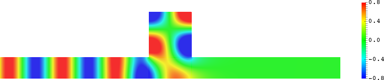
We give examples of waveguides where for well-chosen and . Numerically we set and then we compute for a range of . Finally, we select the such that is maximum. In Figure 12 top, the parameters are set to and (). In Figure 12 bottom, we have and (). As expected, the amplitude of the field is very small in the input lead. In Figure 13, we give another example of geometry where . The waveguide contains two rather large non penetrable obstacles with Neumann boundary condition. Therefore one would expect that some energy would be backscattered. But due to the presence of the vertical branch whose height has been finely tuned, this is not the case and energy is completely transmitted (). In Figure 14, we display a -shaped waveguide where . The geometry is analogous to the one of Figure 18 top right and is unbounded in the left and bottom directions. We play with the length of the diagonal branch. This framework is not exactly the one described in Section 1. However, due to the symmetry, it can be dealt with in a completely similar way.


7.4 Perfect reflectivity
Now in Figures 15 and 16, we provide examples of waveguides where . This time, we select the such that is maximum. In Figure 15 top, the parameters are set to and (). In Figure 15 bottom, we take and (). As expected, the amplitude of the total field is very small in the output lead.


7.5 Perfect invisibility
Finally, we show in Figure 17 an example of waveguide where . We start from the domain
Numerically, first we set and (see the notation in Section 6, Figure 3). Then we approximate the solution of Problem (12) (half-waveguide problem with mixed boundary conditions) for . We select one such that is maximum. Thus we impose . Eventually, we approximate the solution of the initial Problem (2) set in for and we take such that is maximum. We try to cover a range of (relatively) high values of so that remains close to . Indeed, we remind the reader that the error is exponentially small as (see (14)). The parameters are set to , and . As expected, the amplitude of the field is very small both in the input and output leads. Numerically, we obtain a scattering coefficient such that .


8 Concluding remarks
In this article, we have explained how to construct waveguides where non reflectivity (, ), perfect reflectivity (, ) or perfect invisibility (, ) hold. To proceed, we have worked in geometries which are symmetric with respect to the axis and which have one or several vertical branch(es) of finite length. In our presentation, we have always assumed that the branch of finite length is perpendicular to the principal waveguide. Such an assumption is not needed and situations like the ones of Figure 18 top can be considered. We could also investigate settings with truncated periodic waveguides as described in Figure 18 bottom as long as waves can propagate in the vertical branch. Again we mention that we have considered only problems with Neumann boundary condition but higher dimension with other boundary conditions can be dealt with using exactly the same procedure. The analysis we have presented works for the monomode regime (). It seems complicated to extend it to configurations where several propagating modes exist in the horizontal waveguide.
Appendix
In this Appendix, we gather the proofs of two results used in the preceding analysis.
Proposition 8.1.
Proof.
Set and define the segment . Note that the domains , coincide with the strip for . From the expansions (8) and (13) for and , using decomposition in Fourier series, one finds
| (33) |
Define the domain . From the continuity of the trace operator from to (with a constant of continuity independent of ), together with (33), we see that to establish (32), it is sufficient to show the estimate
| (34) |
Here and in what follows is a constant which can change from one line to another but which is independent of . Now we focus our attention on the proof of (34).
First we introduce some notation to reformulate Problem (6) in the bounded domain . Introduce the Dirichlet-to-Neumann map
where is the unique function satisfying
and admitting the expansion . Here and . One can check that is well-defined. Moreover, it is known that is a linear and continuous map from to . Define the space . If is a solution of (6) admitting expansion (8), then solves the problem
| (35) |
with . Here stands for the (bilinear) duality pairing between and . Conversely, if satisfies (35), one can extend as a solution of (6) admitting expansion (8). With the Riesz representation theorem, introduce the bounded operator such that
where denotes the usual inner product of . Under the assumption that the only solution of Problem (12) in is zero (absence of trapped modes), one can show that is invertible for large enough. Moreover there is a constant independent of large enough such that
| (36) |
Here stands for the usual norm on the set of linear operators of . For the proof of this non trivial stability estimate, we refer the reader to [26, Chap. 5, §5.6, Thm. 5.6.3].
We come back to the proof of (34). For large enough, using (36), we can write
| (37) |
Observing that
(we remind the reader that ), we deduce that
| (38) |
Now we assess the right hand side of (38). To proceed, again we need to introduce some notation. For , define the function such that . The family is an orthonormal basis of . Set . Using the equation satisfied by , we obtain the decomposition, for ,
| (39) |
On the other hand, classical results guarantee that for , the norm is equivalent to
| (40) |
with . This allows us to write
Plugging the latter estimate in (38), we deduce
| (41) |
Working on the expansion (39) with formula (40), we can show that
| (42) |
Since , plugging (42) in (41), finally we find
which is nothing but estimate (34). ∎
Proposition 8.2.
The scattering matrix defined in (17) is unitary and symmetric.
Proof.
Define the symplectic (sesquilinear and anti-hermitian ()) form such that for all
Here , on , on and is a given parameter chosen large enough. Moreover, refers to the Sobolev space of functions such that for all bounded domains . Integrating by parts and using that the functions , defined in (16) satisfy the Helmholtz equation, we obtain for . On the other hand, decomposing , in Fourier series on , we find
These relations allow us to prove that , that is to conclude that is unitary. On the other hand, one finds . We deduce that is symmetric. ∎
Acknowledgments
The research of S.A. N. was supported by the grant No. 18-01-00325 of the Russian Foundation on Basic Research. V. P. acknowledges the financial support of the Agence Nationale de la Recherche through the Grant No. DYNAMONDE ANR-12-BS09-0027-01.
References
- [1] G.S. Abeynanda and S.P. Shipman. Dynamic resonance in the high-Q and near-monochromatic regime. MMET, IEEE, 10.1109/MMET.2016.7544100, 2016.
- [2] A. Alù, M.G. Silveirinha, and N. Engheta. Transmission-line analysis of -near-zero–filled narrow channels. Phys. Rev. E, 78(1):016604, 2008.
- [3] A.-S. Bonnet-Ben Dhia, L. Chesnel, and S.A. Nazarov. Non-scattering wavenumbers and far field invisibility for a finite set of incident/scattering directions. Inverse Problems, 31(4):045006, 2015.
- [4] A.-S. Bonnet-Ben Dhia, L. Chesnel, and S.A. Nazarov. Perfect transmission invisibility for waveguides with sound hard walls. J. Math. Pures Appl., 111:79–105, 2018.
- [5] A.-S. Bonnet-Ben Dhia, E. Lunéville, Y. Mbeutcha, and S.A. Nazarov. A method to build non-scattering perturbations of two-dimensional acoustic waveguides. Math. Methods Appl. Sci., 40(2):335–349, 2017.
- [6] A.-S. Bonnet-Ben Dhia and S.A. Nazarov. Obstacles in acoustic waveguides becoming “invisible” at given frequencies. Acoust. Phys., 59(6):633–639, 2013.
- [7] A.-S. Bonnet-Ben Dhia, S.A. Nazarov, and J. Taskinen. Underwater topography “invisible” for surface waves at given frequencies. Wave Motion, 57(0):129–142, 2015.
- [8] E. Bulgakov and A. Sadreev. Formation of bound states in the continuum for a quantum dot with variable width. Phys. Rev. B, 83(23):235321, 2011.
- [9] G. Cardone, S.A. Nazarov, and K. Ruotsalainen. Asymptotic behaviour of an eigenvalue in the continuous spectrum of a narrowed waveguide. Sb. Math., 203(2):153, 2012.
- [10] G. Cattapan and P. Lotti. Bound states in the continuum in two-dimensional serial structures. Eur. Phys. J. B, 66(4):517–523, 2008.
- [11] L. Chesnel, N. Hyvönen, and S. Staboulis. Construction of indistinguishable conductivity perturbations for the point electrode model in electrical impedance tomography. SIAM J. Appl. Math., 75(5):2093–2109, 2015.
- [12] L. Chesnel and S.A. Nazarov. Team organization may help swarms of flies to become invisible in closed waveguides. Inverse Problems and Imaging, 10(4):977–1006, 2016.
- [13] L. Chesnel and S.A. Nazarov. Non reflection and perfect reflection via Fano resonance in waveguides. arXiv preprint arXiv:1801.08889, 2018.
- [14] E.B. Davies and L. Parnovski. Trapped modes in acoustic waveguides. Q. J. Mech. Appl. Math., 51(3):477–492, 1998.
- [15] B. Edwards, A. Alù, M.G. Silveirinha, and N. Engheta. Reflectionless sharp bends and corners in waveguides using epsilon-near-zero effects. J. Appl. Phys., 105(4):044905, 2009.
- [16] D.V. Evans. Trapped acoustic modes. IMA J. Appl. Math., 49(1):45–60, 1992.
- [17] D.V. Evans, M. Levitin, and D. Vassiliev. Existence theorems for trapped modes. J. Fluid. Mech., 261:21–31, 1994.
- [18] D.V. Evans, M. McIver, and R. Porter. Transparency of structures in water waves. In Proceedings of 29th International Workshop on Water Waves and Floating Bodies, 2014.
- [19] U. Fano. Effects of configuration interaction on intensities and phase shifts. Physical Review, 124(6):1866–1878, 1961.
- [20] M. Fernyhough and D.V. Evans. Full multimodal analysis of an open rectangular groove waveguide. Trans. Microw. Theory Techn., 46(1):97–107, 1998.
- [21] R. Fleury and A. Alù. Extraordinary sound transmission through density-near-zero ultranarrow channels. Phys. Rev. Lett., 111(5):055501, 2013.
- [22] Y. Fu, Y. Xu, and H. Chen. Additional modes in a waveguide system of zero-index-metamaterials with defects. Scientific reports, 4, 2014.
- [23] S. Hein, W. Koch, and L. Nannen. Trapped modes and fano resonances in two-dimensional acoustical duct–cavity systems. J. Fluid. Mech., 692:257–287, 2012.
- [24] A.I. Korolkov, S.A. Nazarov, and A.V. Shanin. Stabilizing solutions at thresholds of the continuous spectrum and anomalous transmission of waves. Z. Angew. Math. Mech., 96(10):1245–1260, 2016.
- [25] C.M. Linton and P. McIver. Embedded trapped modes in water waves and acoustics. Wave motion, 45(1):16–29, 2007.
- [26] V.G. Maz’ya, S.A. Nazarov, and B.A. Plamenevskiĭ. Asymptotic theory of elliptic boundary value problems in singularly perturbed domains, Vol. 1. Birkhäuser, Basel, 2000. Translated from the original German 1991 edition.
- [27] N. Moiseyev. Suppression of Feshbach resonance widths in two-dimensional waveguides and quantum dots: a lower bound for the number of bound states in the continuum. Phys. Rev. Lett., 102(16):167404, 2009.
- [28] S.A. Nazarov. Sufficient conditions on the existence of trapped modes in problems of the linear theory of surface waves. J. Math. Sci., 167(5):713–725, 2010.
- [29] S.A. Nazarov. Trapped modes in a T-shaped waveguide. Acoust. Phys., 56(6):1004–1015, 2010.
- [30] S.A. Nazarov. Asymptotic expansions of eigenvalues in the continuous spectrum of a regularly perturbed quantum waveguide. Theor. Math. Phys., 167(2):606–627, 2011.
- [31] S.A. Nazarov. Eigenvalues of the Laplace operator with the Neumann conditions at regular perturbed walls of a waveguide. J. Math. Sci., 172(4):555–588, 2011.
- [32] S.A. Nazarov. Trapped waves in a cranked waveguide with hard walls. Acoust. Phys., 57(6):764–771, 2011.
- [33] S.A. Nazarov. Enforced stability of an eigenvalue in the continuous spectrum of a waveguide with an obstacle. Comput. Math. and Math. Phys., 52(3):448–464, 2012.
- [34] S.A. Nazarov. Enforced stability of a simple eigenvalue in the continuous spectrum of a waveguide. Funct. Anal. Appl., 47(3):195–209, 2013.
- [35] S.A. Nazarov. Scattering anomalies in a resonator above thresholds of the continuous spectrum. Mat. sbornik., 206(6):15–48, 2015. (English transl.: Sb. Math. 2015. V. 206. N 6. P. 782–813).
- [36] S.A. Nazarov and B.A. Plamenevskiĭ. Elliptic problems in domains with piecewise smooth boundaries, volume 13 of Expositions in Mathematics. De Gruyter, Berlin, Germany, 1994.
- [37] S.A. Nazarov and A.V. Shanin. Calculation of characteristics of trapped modes in t-shaped waveguides. Computational Mathematics and Mathematical Physics, 51(1):96–110, 2011.
- [38] S.A. Nazarov and J.H. Videman. Existence of edge waves along three-dimensional periodic structures. J. Fluid. Mech., 659:225–246, 2010.
- [39] V.C. Nguyen, L. Chen, and K. Halterman. Total transmission and total reflection by zero index metamaterials with defects. Phys. Rev. Lett., 105(23):233908, 2010.
- [40] A. Ourir, A. Maurel, and V. Pagneux. Tunneling of electromagnetic energy in multiple connected leads using -near-zero materials. Opt. Lett., 38(12):2092–2094, 2013.
- [41] R. Porter and J.N. Newman. Cloaking of a vertical cylinder in waves using variable bathymetry. J. Fluid Mech., 750:124–143, 2014.
- [42] S.P. Shipman and H. Tu. Total resonant transmission and reflection by periodic structures. SIAM J. Appl. Math., 72(1):216–239, 2012.
- [43] S.P. Shipman and S. Venakides. Resonant transmission near nonrobust periodic slab modes. Phys. Rev. E, 71(2):026611, 2005.
- [44] S.P. Shipman and A.T. Welters. Resonant electromagnetic scattering in anisotropic layered media. J. Math. Phys., 54(10):103511, 2013.
- [45] F. Ursell. Trapping modes in the theory of surface waves. Proc. Camb. Philos. Soc., 47:347–358, 1951.
- [46] L.A. Vainshtein. Diffraction theory and the factorization method. Sov. Radio, Moscow, 1966. (Russian).