Extended chiral Khuri-Treiman formalism for and the role of the , resonances
Abstract
Recent experiments on decays have provided an extremely precise knowledge of the amplitudes across the Dalitz region which represent stringent constraints on theoretical descriptions. We reconsider an approach in which the low-energy chiral expansion is assumed to be optimally convergent in an unphysical region surrounding the Adler zero, and the amplitude in the physical region is uniquely deduced by an analyticity-based extrapolation using the Khuri-Treiman dispersive formalism. We present an extension of the usual formalism which implements the leading inelastic effects from the channel in the final-state interaction as well as in the initial-state interaction. The constructed amplitude has an enlarged region of validity and accounts in a realistic way for the influence of the two light scalar resonances and in the dispersive integrals. It is shown that the effect of these resonances in the low energy region of the decay is not negligible, in particular for the mode, and improves the description of the energy variation across the Dalitz plot. Some remarks are made on the scale dependence and the value of the double quark mass ratio .
1 Introduction
The physics of QCD in the soft regime is dominated by the phenomenon of spontaneous symmetry breaking because of the presence of three light quarks in the standard model. The low-energy dynamics can then be described accurately through an expansion built from a chiral effective theory (e.g. [1] for a recent review). This approach, which applies in both the Euclidean and Minkowski space-times is, to some extent, complementary to the purely numerical lattice simulation method. In the effective theory, however, part of the information on the non-perturbative QCD dynamics is contained as sets of values of the chiral coupling constants. These are not known, a priori, except for their order of magnitude [2] and must be determined as part of the probing of the effective theory.
In QCD, isospin breaking phenomena are driven by , the mass difference of the two lightest quarks. For low-energy observables, an isospin breaking ratio which conveniently absorbs some of the next-to-leading (NLO) chiral coupling constants was introduced in ref. [3]
| (1) |
In general, isospin breaking effects induced by electromagnetism are comparable in size to those proportional to and their precise evaluation is made difficult by the poor knowledge of the associated chiral coupling constants [4]. In this respect, the amplitude plays a special role because these electromagnetic contributions vanish in the chiral limit [5] and are thus expected to be suppressed. This has been confirmed in the work of refs. [6, 7] who evaluated the contributions proportional to , .
A number of recent high-statistics experiments have studied the decay mode of the [8, 9, 10, 11, 12] as well as the charged mode [13, 14, 15, 16]. An extremely precise knowledge of the energy variation of the amplitudes squared across the Dalitz plot, which are traditionally represented by a set of polynomial parameters, has now become available. These accurate experimental results allow for stringent tests of the theoretical description of the amplitude which must obviously be passed before one attempts to determine . The Dalitz plot parameters derived directly from the NLO chiral amplitude, which was first computed in [17], are in clear disagreement with experiment. For instance, the prediction for the parameter , involved in the neutral mode, has the wrong sign. The same problems, essentially, are found in the resummed expansion approach discussed recently in ref. [18]. The computation of the amplitude at the next-to-next-to leading (NNLO) chiral order was performed [19]. The comparison with experiment again fails if one assumes a simple naive model for the couplings (classified in ref. [20]) which are involved as six independent combinations. The decay amplitude thus contains crucial information on the true QCD values of these couplings, which are essentially not known at present.
One obvious deficiency of the chiral expansion when calculating scattering or decay amplitudes in physical regions is the lack of exact unitarity (as emphasised e.g. in ref. [21]) which is restored gradually when going to higher orders. In the case of , a large amount of work was devoted to the problem of estimating these unitarity, or final-state rescattering, higher order corrections [22, 23, 24, 25, 26, 27, 28].
In the present paper we reconsider, more specifically, the approach followed in refs. [22, 24, 25]. The main underlying assumption is that the chiral expansion of the decay amplitude should be optimally converging in an unphysical region of the Mandelstam plane in the neighbourhood of the Adler zero. The amplitude in the physical region is then deduced from a well-defined extrapolation procedure based on the analyticity properties of amplitudes in QCD, which utilise the set of dispersive equations derived initially by Khuri and Treiman [29] and perfected in the work of refs. [22, 24, 25]. These equations implement crossing-symmetry and unitarity in a more complete way than more naive loop-resummation approaches [26].
In previous work, rescattering was assumed to be elastic. This is essentially exact in the physical decay region. However, the dispersive formalism involves integrals over an energy range extending up to infinity. A property of the scattering amplitude in the isoscalar S-wave is the sharp onset of inelasticity associated with the scalar resonance [30, 31]. Because of isospin violation, the amplitude actually exhibits a double resonance effect from both the and the scalars [32] near the threshold. Our aim is to propose a generalisation of the Khuri-Treiman formalism which takes into account inelasticity in the unitarity relations for both scattering and scattering (which may be viewed as an initial-state interaction). Some approximations will be made, which simplify considerably the practical implementation, such that crossing-symmetry is maintained at the level of the amplitudes but not in the amplitudes involving the channel. In this multichannel formalism, the double resonance effect is taken into account in the dispersive integrals and, furthermore, the construction of the amplitude becomes valid in an extended energy region which includes not only the decay region but also a portion of the scattering region. This will allow us to study how the energy dependence induced by the two 1 GeV scalar resonances propagate down to the low energy region and quantitatively affects the Dalitz plot parameters. The fact that these resonances could be influential at low energy was pointed out previously in ref. [33].
The plan of the paper is as follows. We first review in sec. 2 the derivation of the one-channel equations in which the amplitudes satisfy elastic unitarity in the and the -waves. In sec. 3 we write the unitarity relations including the and the channels. A closed system of unitarity equations involves, besides , isospin violating components of , as well as amplitudes. A multichannel set of Khuri-Treiman integral equations is defined such that the solution amplitudes satisfy these unitarity relations. We then discuss in sec. 4 the matching between the chiral expansion amplitudes and the dispersive ones. We adopt a simple approach which consists in imposing that the difference between the chiral NLO and dispersive amplitudes vanishes at order . This provides four equations which, in the single-channel case determine completely the dispersive amplitude provided one had introduced exactly four polynomial parameters in the Khuri-Treiman representation. This is generalised to the multichannel situation, in which one introduces 16 polynomial parameters. Finally, in sec. 5, the results on the Dalitz plot parameters are presented and some remarks are made on the determination of the quark mass ratio .
2 Khuri-Treiman equations in the elastic approximation
We remind below how the dispersion relations-based equations derived by Khuri and Treiman [29] for decay can be generalised and applied to , following [22, 24, 25].
2.1 Single-variable amplitudes for
As initially demonstrated in the case of (see [34]), amplitudes involving four pseudo-Goldstone bosons satisfy, in a certain kinematical range, an approximate representation in terms of functions of a single variable which have simple analyticity properties (see [35] for a review). In the case of , and neglecting quadratic isospin breaking, there are three functions involved [24, 25]: , , . We will follow the notation of ref. [25] and write the amplitude as
| (2) |
with an overall factor11 1 It is convenient to formally factor out but the amplitude is actually of the form: where is the electric charge and is the physical mass squared difference (see appendix A). which is proportional to the isospin breaking double quark mass ratio given in eq. (1)
| (3) |
The Mandelstam variables are defined, as usual, as
| (4) |
and satisfy
| (5) |
General analyticity properties imply that decay and scattering are described by the same function in different regions of the Mandelstam plane. The corresponding physical regions are illustrated in fig. 1. The analogous representation for involves the two functions and only and reads
| (6) |

The representations (2) and (6) are accurate in regions of the Mandelstam plane where the imaginary parts of the partial-wave amplitudes with angular momentum in the , or channels are negligible (compared to those of the partial-waves). In the case of or , this condition is satisfied in the range where , , are sufficiently small compared with the masses squared of the tensor resonances, i.e. . This condition is also satisfied exactly by the amplitude obtained from the chiral expansion up to order [19]. This will prove very useful for writing matching conditions.
The functions are analytic in with a cut on the positive real axis: . Based on Regge theory, we expect that the functions and should not grow faster than at infinity, while should be bounded by a constant. In the one-channel Khuri-Treiman framework, both and are usually assumed to behave linearly in when . With this asymptotic behaviour, there is a family of redefinitions of the functions and which leaves the physical amplitude unmodified [25, 36],
| (7) |
(, , being arbitrary constant parameters) provided one correspondingly redefines as
| (8) |
with
| (9) |
and using the constraint (5). This arbitrariness can be fixed by imposing the three conditions
| (10) |
In the coupled-channel set-up, to be discussed below, the asymptotic condition on will be modified such that goes to a constant when instead of behaving linearly. This restricts the allowed redefinitions of , to those which satisfy . In that case, only the two conditions can be imposed, while is determined from the equations.
These properties of the functions lead to the following dispersive representations
| (11) |
defining
| (12) |
2.2 Isospin amplitudes and crossing relations
We choose the following conventional isospin assignment for the pions and the kaons
| (13) |
Let us consider the amplitudes which correspond to isospin states of the system,
| (14) |
One can express in terms of isospin amplitudes,
| (15) |
Further relations for the isospin amplitudes can be obtained using crossing symmetries. Under and crossing one obtains,
| (16) |
Since the isospin breaking operator in QCD, , transforms as , , one can use the Wigner-Eckart theorem
| (17) |
which yields the following relations among the amplitudes
| (18) |
One can then express the three independent isospin amplitudes in terms of the function
| (19) |
In the following we will simply denote
| (20) |
Inserting the representation (2) we obtain an expression of the three isospin amplitudes in terms of the one-variable functions
| (21) |
2.3 Partial-waves and elastic unitarity relations
In order to derive expressions for the discontinuities , we must consider partial-waves and their unitarity relations. We can define the partial-wave expansion of the isospin amplitudes as
| (22) |
where is the cosine of the scattering angle in the centre-of-mass frame of which is related to the Mandelstam variables by
| (23) |
with
| (24) |
From the representation of the isospin amplitudes, eq. (21) one easily derives the expression for the partial-waves. The result, for the partial-waves, can be written as,
| (25) |
where the functions are given by linear combinations of angular integrals of the functions
| (26) |
with the notation [25]
| (27) |
Writing unitarity relations, one must first consider the unphysical situation where the meson is stable, . The physical case is defined using analytic continuation in as in the classic derivation of generalised unitarity [37]. The contribution from the states to the unitarity relation for the partial-wave , reads
| (28) |
with
| (29) |
and is the partial-wave amplitude, which is related to the scattering phase-shift by
| (30) |
The equality between the imaginary part and the discontinuity in eq. (28) holds when . For the physical value of the right-hand side of eq. (28) continues to give the discontinuity across the unitarity cut, while the imaginary part must be deduced from the dispersive representation.
2.4 Khuri-Treiman equations in the elastic approximation
In the unphysical situation when , the cuts of the functions are located in the region such that eqs. (25) correspond to a splitting of the partial wave amplitudes into two functions which have a separated cut structure. When the mass is increased to its physical value, the prescription must be used [37] and this insures that the complex cut of the functions, which approaches infinitesimally close to the unitarity cut in the region , remains well separated from it (see fig. 4 in ref. [38]). Using the fact that has no discontinuity across the unitarity cut one can deduce from (28) that the discontinuities of the functions along are given by
| (31) |
where when and when . In the sequel, we will drop the subscript in the phase-shift. Eqs. (31) imply that the functions can be written as Muskhelishvili-Omnès (MO) integral representations
| (32) |
where
| (33) |
and where the Omnès functions are given in terms of the phase-shifts by the usual relation
| (34) |
The phase-shifts, in the present context, are usually taken to obey the following asymptotic conditions
| (35) |
which seem rather natural since these conditions are roughly satisfied at the threshold. In the elastic approximation framework, one can thus take the phases to be constant or quasi-constant in the inelastic region, above 1 GeV.
The polynomial part in the MO representation (32) was chosen to have four parameters. This allows one to define a unique dispersive amplitude by implementing four independent matching conditions with the chiral NLO amplitude. Taking into account the asymptotic conditions on the phase-shifts (35) one easily sees that the Khuri-Treiman equations (32) implement the following asymptotic behaviour for the functions
| (36) |
The functions also satisfy the conditions (10) and are thus uniquely defined.
3 Beyond the elastic approximation
Elastic unitarity for scattering is valid exactly below the four pions threshold and approximately up to the threshold. Close to 1 GeV, the phase-shift increases very sharply under the influence of the resonance which also couples strongly to . In order to properly account for the effect of this resonance it is thus necessary to go beyond the elastic unitarity approximation. We discuss in this section how to include both the and the channels into the unitarity relations and then generate a generalisation of the Khuri-Treiman equations. This will allow us to account for both the and the resonances in a realistic way.
3.1 contribution to unitarity
Including the channel in addition to , the unitarity relation becomes
| (37) |
where
| (38) |
and is the partial-wave amplitude. In the energy region where scattering is elastic, which we will assume to extend up to the threshold, is related to the scattering phase-shift by
| (39) |
The partial-wave corresponds to exotic quantum numbers and should thus remain rather small up to the 1 GeV region22 2 A resonance possibly exists in this amplitude [39] with a mass GeV. Therefore, rescattering is expected to affect mainly the two amplitudes and . In the elastic regime, using eq. (37) one easily derives that the relation between the amplitudes on both sides of the unitarity cut reads,
| (40) |
Comparing with the analogous relation in the elastic unitarity case (28) one deduces that including the effect of rescattering in the amplitude (which can be viewed as an initial-state interaction) amounts to simply perform the following replacements in the Omnès representations (32),
| (41) |
In practice, rescattering is expected to become significant when the energy approaches the mass of the resonance. It becomes necessary, then, to also take into account the channel.
3.2 contributions to unitarity
Let us now include the states into the partial-wave unitarity relations.
- a)
: We are concerned mainly with amplitudes but let us consider the amplitude here also for completeness. The contribution reads
(42) The amplitude is isospin violating33 3 The amplitudes are isospin violating (conserving) for odd (even) values of . This can be seen using G-parity: . Since for , for odd values of and for even values while for . and, at linear order in isospin breaking, one can set . We will denote the amplitudes appearing above as
(43) - b)
: For the amplitude now, the contribution reads
(44) The amplitude is isospin conserving in this case, since is even while the amplitude is isospin violating. We will denote the two amplitudes in eq. (44) as
(45) - c)
: Finally, for the amplitude, the contributions to the unitarity relations are
(46)
Let us now separate the isospin conserving and the isospin violating contributions. For the kinematical factors, we introduce
| (47) |
For the amplitudes, the isospin conserving part, , was introduced in eq. (45) and we call the isospin violating one . One has
| (48) |
For the amplitudes, the isospin conserving and the isospin violating amplitudes are denoted as
| (49) |
Using this notation, the contributions in the unitarity relations for the partial-waves can be summarised as follows
| (50) |
These contributions involve new isospin-breaking and amplitudes: , , , . In order to write a closed set of unitarity equations we must also consider amplitudes. For these, the isospin conserving/violating components are denoted ,
| (51) |
Table 1 summarises our notation for the various amplitudes involved.
| cons. | viol. | |
|---|---|---|
4 Multichannel Khuri-Treiman equations
4.1 Closed system of unitarity equations
We can now write down a closed system of unitarity equations. It will be convenient to introduce a matrix notation for the isospin conserving amplitudes with and
| (52) |
The amplitude is now embedded into a system of four coupled unitarity equations
| (53) |
where
| (54) |
while the amplitude is involved in a system of two unitarity equations,
| (55) |
Finally, for the amplitude , the coupled unitarity equations read
| (56) |
In the following, however, we will disregard the inelasticity effects for and continue to use the elastic unitarity equation (28) in this case.
4.2 Coupled Muskhelishvili-Omnès representation
The next step is to write each one of the isospin violating partial-wave amplitudes as a sum of two functions, one having a right-hand cut only and one having a generalised left-hand cut. For physical mass values, the left and right-hand cuts of the various partial-waves appear to be overlapping, but it is possible to separate them unambiguously. In the case of the amplitudes involving the meson, this is done by using the prescription. The amplitude has a left-hand cut which extends on the real axis in the range . Using the prescription shifts this cut above the real axis.
For the amplitudes one writes
| (57) |
which generalises eq. (25) while for the amplitudes one can write
| (58) |
One can now employ the standard Omnès method in order to express the right-cut functions in terms of the left-cut ones. Introducing the matrix notation
| (59) |
the discontinuity relation for the functions is deduced from the unitarity relation (53),
| (60) |
where
| (61) |
and is given in eq. (47). Eq. (60) generalises the one-channel discontinuity relation (31).
Let us now consider the following matrix
| (62) |
where are the Muskhelishvili-Omnès matrices corresponding to the -matrices . Making use of the following discontinuity properties of the MO matrices
| (63) |
one can express the discontinuity of the matrix elements in terms of the functions and
| (64) |
where
| (65) |
An alternative expression for can be derived, using eqs. (63))
| (66) |
which shows that it represents the discontinuity of the following quantity
| (67) |
across the right-hand cut. The quantity is proportional to and it is given by
| (68) |
We can then write a twice subtracted dispersive representation for and generate, via (62), a MO representation for the amplitudes
| (69) |
where is a matrix of polynomial functions,
| (70) |
and the integral parts are
| (71) |
One remarks that in the term the quark mass ratio appears in the denominator and thus cancels with the overall factor in the complete amplitudes. This part is driven by the physical mass difference via the function (see (47)). This mechanism was first studied in ref. [32] who predicted that a large isospin violation should take place at 1 GeV in the scattering amplitude, due to the contributions from both the and the resonances. The set of eqs. (69) account for the other sources of isospin violation as well.
We now consider the case of the amplitudes and we also introduce a matrix notation for the column matrices
| (72) |
From the unitarity relations including the , and contributions we deduce the discontinuity of the functions
| (73) |
As before, we introduce a matrix , multiplying by inverse MO functions,
| (74) |
Its discontinuity relation is expressed in terms of the functions and the MO functions
| (75) |
An alternative useful expression for can be derived
| (76) |
This leads to the following integral MO representation for the matrix ,
| (77) |
with
| (78) |
Eqs. (69) and (77) together with the uncoupled equation for (32) involve 16 polynomial parameters. The polynomial dependence was chosen such that the equations would reduce exactly to the set of elastic equations (32) if one switches off the coupling to the channel as well as rescattering44 4 The one-channel case is recovered by setting and the MO matrices to and .. One remarks that the asymptotic behaviour in the coupled-channel equations is modified as compared to the one-channel case: since the matrix elements of the MO matrices , decrease as when goes to the entries of the matrix (thus the function) behave as constants. The asymptotic behaviour of , in contrast, remains the same as before.
In addition to the polynomial parameters, the right-hand side of eqs. (69), (77) involve a number of “hat functions”. The functions are determined in terms of the functions by the angular integrals (26), but one still needs to determine the other hat functions , , , which are related to the amplitudes. For this purpose, one would have to consider all the related crossed channel amplitudes an write similar sets of equations (which would introduce further one-variable functions). Here, since we are mainly interested in the amplitude we will content with an approximation for the amplitudes involving the channel, simply neglecting the integrals which involve the left-cut functions, i.e. we take
| (79) |
In support of this approximation, one observes that if one were to neglect the left-cut integrals in the amplitude itself, one would still obtain a qualitatively reasonable description (e.g. [40]). With this approximation, eqs. (69) and (77) constitute a closed set of equations which form a coupled-channel generalisation of the Khuri-Treiman equations (32) for and .
4.3 Matching to the chiral amplitudes
We intend to fix the 16 polynomial parameters by matching to the chiral expansions of the amplitudes involved. For the amplitude we will use the NLO expansion also including the part of the electromagnetic contributions of order from ref. [6]. This makes it possible to display explicitly the term induced by the mass difference via unitarity which, in the dispersive representation, is contained in the integrals (see eqs. (68), (71)). The explicit chiral expressions for the functions as used here are given in appendix A.
For the isospin violating amplitudes involving the channel we will use the leading order chiral expansion. At this order, the partial-wave amplitudes have no left-hand cut, which is consistent with the approximation of dropping the left-cut functions in the integral equations. The relevant expressions (including the contributions) are given below
| (80) |
with
| (81) |
and the coupling constant can be related to the mass difference (see appendix A).
We implement matching conditions for the amplitude following the simple method of ref. [38] which differs slightly from that of ref. [25]. Let be the amplitude computed in the chiral expansion at order . The polynomial parameters of the dispersive amplitude must be determined such that the dispersive and chiral amplitudes coincide for small values of the Mandelstam variables. At order one should thus have
| (82) |
This condition is satisfied automatically for the discontinuities, which implies that one can neglect the discontinuity of the differences of the one-variable functions and thus expand these differences as polynomials,
| (83) |
(with , ). Inserting these expansions into the amplitude difference and requiring that the polynomial part vanishes gives four equations. In the elastic Khuri-Treiman framework these determine the four parameters via the following four equations
| (84) |
with
| (85) |
and one must keep in mind that the integrals which appear on the right-hand sides depend linearly on the four parameters. In ref. [25] the first two of eqs. (84) were replaced by two equations related to the position of the Adler zero of the chiral amplitude along the line and the value of its derivative at . We will see below that eqs. (84) do actually implement these Adler zero conditions to a rather good approximation. Additionally, approximations were made in ref. [25] in the determination of and (yielding e.g. ), the validity of which depends on the assumed behaviour of the phase in the inelastic region. Here, the four equations will be solved without approximation. Doing so, one notes that the polynomial parameters get an imaginary part from the contributions of the integrals which, however, is small (less that 10% of the real part).
In the coupled-channel case, the matching of the amplitude again gives rise to four equations. In addition, we can match the values at of each one of the four amplitudes with the chiral ones given in eqs. (80) as well as the values of the first and second derivatives (which are vanishing). Altogether, this provides 16 constraints which fix all the polynomial parameters appearing in the coupled-channel Khuri-Treiman equations. The details of these matching equations are given in appendix B.
5 Results and comparisons with experiment
5.1 Numerical method
The main difficulty which is involved in deriving accurate numerical solutions of the Khuri-Treiman equations is tied to the evaluation of the angular integrals needed to obtain the hat functions and to the treatment of the singularities of these functions in the computation of the integrals which are finite. These technical aspects are discussed in detail in ref. [24]. By a change of variables one can rewrite the angular integrals as integrals over
| (86) |
with
| (87) |
When lies in the range , the endpoints become complex. In fact, using the prescription one sees that and are placed on opposite sides of the unitarity cut when gets larger that . The integral from to must then be evaluated along a complex contour which circles around the unitarity cut of the functions . Rather than computing explicitly for complex values of , as in ref. [24], we follow here the approach of ref. [38] which consists in inserting the dispersive representations (11) of the functions into eq. (86) and computing analytically the integrals. This makes it possible to express the functions in terms of the discontinuities along the positive real axis. The relevant formulae are recalled in appendix C.
The equations are conveniently solved using an iterative procedure. On the first iteration step, one sets the functions equal to zero. Then the integrals are also equal to zero and it is straightforward to compute the values of the polynomial parameters from the matching equations and then the functions , , , , as well as the discontinuities (which are given from eqs. (31) in the one-channel case and (60) (73) in the coupled-channel case). The coupled-channel framework is somewhat more complicated to handle than the single-channel one, essentially because the MO matrices do not obey a simple explicit representation in terms of the -matrix elements and must be solved for numerically, but does not otherwise involve any specific difficulty. Then, on each iteration step, one updates the values of the functions using from the preceding step, and then compute the integrals. Then, one updates the values of the polynomial parameters and derive the new values of all the functions , , , , and those of discontinuities .
Convergence is found to be reasonably fast. Denoting by the result obtained at the iteration step we can estimate the rate of convergence from the quantity
| (88) |
Anticipating on the numerical results to be presented below, with we find: , , . The amplitude is the one which has the slowest convergence rate.


5.2 Input T-matrices
Above the threshold, the and matrices are related by
| (89) |
Two-channel unitarity implies that all the -matrix elements are determined from three real inputs: a) the phase of , b) the modulus of and c) the phase of . For scattering, experimental data exist for these quantities up to 2 GeV, approximately. We will use here a determination based on the experimental data of Hyams et al. [41] for the phase-shifts and the data of refs. [42] and [43] (above 1.3 GeV) for the amplitude55 5 We note, however, that a recent analysis of the Roy equations in a once-subtracted version[44] shows some tension with the data of Cohen et al. [42] assuming that it saturates inelasticity near the threshold.. In the higher energy region, a smooth interpolation is performed with the following asymptotic conditions,
| (90) |
which insure (in general) the existence of a corresponding unique MO matrix [45]. Below the threshold, a determination of the phase-shift based on the data of ref. [41] together with constraints from the Roy equations (in the twice-subtracted version of ref. [46]) is performed. It is assumed that inelasticity can be neglected in this region, which implies that the phase of the amplitude coincides with the phase-shift (Fermi-Watson theorem). This allows one to determine the modulus of this amplitude below the threshold [47] where it is also needed. Details on the parametrisation can be found in refs. [48, 49]. Fig. 2 shows the experimental data used and the fitted curves.


In the case of the -matrix, experimental information on and scattering are indirect and far less detailed than for . We will rely here on the chiral -matrix model proposed in ref. [50] which provides a simple interpolation between certain known properties of the prominent scalar resonances and and the low energy properties constrained by chiral symmetry. The -matrix reproduces, by construction, the and chiral amplitudes at NLO (and more approximately the amplitude ). It depends on the values of the chiral couplings: we use here (as in ref. [50]) a set of values for these taken from a fit of ref. [51]. We note that the value of in this set is . We will use this value also in the computation of the amplitude, for consistency.
A further constraint can be implemented by computing the and scalar form-factors from this -matrix. Chiral symmetry relates the and the scalar radii, which leads to the prediction that should be remarkably small, . This small value can be reproduced provided the phase raises sufficiently slowly above the threshold. The phenomenological parameters of the model are also constrained by the properties of the resonances. Fig. 3 shows a typical result for the phase shift and for the phase and modulus of the amplitude66 6 The phase shown is that of (according to the isospin convention of eq. (13)). It satisfies which corresponds to , within 20% of the chiral result. which we will use in the present work.


Finally, the phase shifts which we used for the -wave and the -wave, for which inelasticity is ignored, are shown in fig. 4. In the energy region GeV, these phase shifts are given by the Roy equations solution parametrisation of ref. [46]. They are fitted to experimental data from [41] (-wave) and [52, 53] () in the region GeV and interpolated to , in the higher energy region.
5.3 Illustration of the role of the inelastic channels


Results for the amplitude obtained from solving numerically the Khuri-Treiman equations are presented in fig. 5 which shows the real part of the amplitude along the line as a function of . Let us consider the role of the inelastic channels in four energy regions
- a)
In the neighbourhood of there is a very sharp energy variation, as one could have easily expected, induced by the interference of the and resonances and the presence of the and thresholds.
- b)
In the region the coupled-channel amplitude displays a large enhancement as compared to the single-channel amplitude.
- c)
In the lower energy region, , on the contrary, the effect of the inelastic channels is to reduce the size of the amplitude. One also observes that in this region the influence of the inelastic channels becomes small.
- d)
In the sub-threshold region, finally, the coupled-channel and single-channel amplitudes are essentially indistinguishable. This is expected since the amplitudes are constrained to satisfy the same chiral matching equations.

It is not difficult to identify the main mechanism which generates the behaviour described above. For this purpose, let us consider the component of the matrix and let us absorb the the effect of the integrals , at into the polynomial matrix, defining
| (91) |
The real parts of the three components of which are related to the channel have the following expressions
| (92) |
These polynomial coefficients are controlled, we recall, by the matching conditions to the LO chiral , , and isospin violating amplitudes (see appendix B). The component is negative in the region and dominates the others in the range . In fact, the corresponding contribution to dominates in the whole region . In this region, the contribution from the inelastic channels can thus be written approximately as
| (93) |
The components of the Omnès matrices which appear in eq. (93) are plotted in fig. 6. The salient feature here is that the real part of the component is positive at low energy and changes sign77 7 The presence of a zero below the threshold follows from Watson’s theorem which is obeyed by the component and leads to the relation . This implies that vanishes when the phase shift goes through . at . This is the main reason why the inelastic channels decrease the amplitude below and increase it above. This behaviour is enhanced by the component which is larger than 1 (reflecting the attractive nature of the interaction below 1 GeV).

The behaviour of the amplitude along the (or ) line, which displays the Adler zero, is shown in fig. 7. In the sub-threshold region, the chiral, the single-channel and the coupled-channel amplitudes are seen to be very close. For the position of the Adler zero, we find
| (94) |
Finally, the results for the amplitude are shown in fig. 8. The influence of the inelastic channels are seen to be quite substantial in this case in the whole low-energy region. One also sees that there is no region in which there is close agreement between the dispersive and the chiral amplitudes. This, of course, is because of the occurrence of the combination and the fact that at least one of the variables , , must lie above the threshold, thus generating significant -wave rescattering chiral corrections.

5.4 Dalitz plot parameters
One traditionally describes the Dalitz plot in terms of two dimensionless variables , such that and the centre of the Dalitz plot corresponds to . In the case of the charged decay amplitude , the variables , are related to the Mandelstam ones by
| (95) |
with . Assuming charge conjugation invariance, the amplitude must be invariant under the transformation and a polynomial parametrisation of the amplitude squared can be written as
| (96) |
In the case of the neutral decay amplitude , must be replaced by in the definition of and . Charge conjugation and Bose symmetry imply that the amplitude must be invariant under the two transformations
| (97) |
with . The amplitude squared can thus be represented as
| (98) |
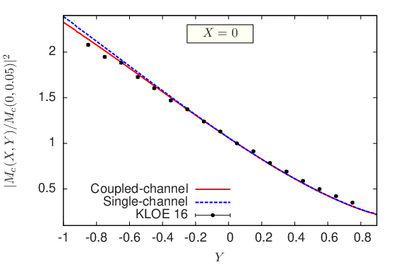
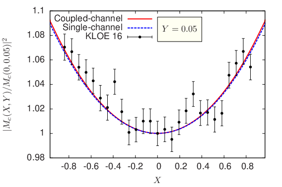
A direct comparison of the dispersive amplitudes squared with the experimental data from KLOE [16] is shown in fig. 9 and our numerical results for the Dalitz plot parameters are collected in table 2. The numbers quoted in the table are obtained in a way which parallels the experimental determination: a discrete binning of the Dalitz plot is performed (with a few hundred bins) and a global least squares fit of the theoretical (chiral or dispersive) amplitudes squared is performed using the representations (96), (98). The table also shows the two most recent experimental determinations [15, 16].
| single-ch. | coupled-ch. | KLOE | BESIII | ||
| a | -1.328 | -1.156 | -1.142 | -1.095(4) | -1.128(15) |
| b | 0.429 | 0.200 | 0.172 | 0.145(6) | 0.153(17) |
| d | 0.090 | 0.095 | 0.097 | 0.081(7) | 0.085(16) |
| f | 0.017 | 0.109 | 0.122 | 0.141(10) | 0.173(28) |
| g | -0.081 | -0.088 | -0.089 | -0.044(16) | – |
| PDG | |||||
| +0.0142 | -0.0268 | -0.0319 | -0.0318(15) | ||
| -0.0007 | -0.0046 | -0.0056 | |||
It is clear, at first, that the amplitudes obtained from solving the Khuri-Treiman equations and constrained to match the chiral NLO amplitudes are in much better agreement with the experimental results in the physical decay region than the NLO amplitude itself. In particular, the parameter which was too large by a factor of three is reduced by a factor of two and the parameter which was positive becomes negative. This is in close agreement with the results obtained a long time ago by Kambor et al. [24]. Our main new result is that taking into account the inelastic channels and the effect of rescattering has a non negligible influence on the Dalitz parameters and tends to further improve the agreement with experiment. The influence of these inelastic channels for the parameters and is small (less than 5%) but quite significant for the parameter which is reduced by 17% and now lies within 15% of the experimental value. This reflects the reduction of the amplitude caused by the inelastic effects at low energy discussed in sec. 5.3. Similarly, the parameter is modified by approximately 20% by the inelastic channels and becomes rather close to the experimental result. The parameter is the only one which shows a mismatch, by a factor of two, with the value measured by KLOE.
Finally, let us consider the sensitivity of the Dalitz plot parameters to the strength of the interaction, which is not precisely known at present. This is illustrated in table 3. The table also shows that varying the coupling has a significant influence, in particular on the parameter .
| no | large | ||
|---|---|---|---|
5.5 The ratio
Let us quote here the results for the ratio of the and the decay rates
| (99) |
We find that the influence of the inelastic channels on this ratio is very small,
| (100) |
As compared with the chiral result
| (101) |
this ratio is thus predicted to increase under the effect of the final-state interactions, by only 2%. The experimental status of this quantity is not completely clear at present, as the PDG[54] quotes two different numbers
| (102) |
Besides, the CLEO collaboration [56] has performed an experiment dedicated to the determinations of the meson decay branching fractions and they quote
| (103) |
as the most precise determination of the ratio.
5.6 The quark mass ratio from the chirally matched dispersive amplitude
It must first be reminded that, once the electromagnetic interaction is taken into account, the quark mass ratio is no longer invariant under the QCD renormalisation group since the quark mass variation with the scale depends on its electric charge
| (104) |
(with , ). This implies the following scale variation for the factor
| (105) |
It can then easily be verified, using the equations of appendix A which include the contributions [6], that the scale invariance of the complete NLO chiral amplitude is restored thanks to the combination of two of the electromagnetic coupling constants [4], . Indeed, as shown in refs. [57, 58] this combination depends not only on the chiral scale but also on the QCD scale and satisfies
| (106) |
In practice, this means that in order to determine from the amplitude we must specify the values of the electromagnetic chiral couplings at the corresponding scale. We choose here GeV and estimate the values of the couplings from a resonance saturation model [59]. Such estimates are qualitative at best but it can be shown, based on general order of magnitude arguments, that the uncertainty induced on the amplitude should not exceed a few percent [6, 7].
Having verified that the dispersive amplitude is in qualitative agreement with experiment concerning the Dalitz plot parameters, we can make an estimate of the value of . In the present approach, the amplitude in the physical decay region is derived as a Khuri-Treiman solution uniquely defined from the chiral NLO amplitude by the set of four matching equations, and thus has a definite dependence on . We can then estimate the value of by the requirement that the dispersive amplitude reproduces the experimental values of the decay widths
| (107) |
taken from the PDG [54] (constrained fit). Doing this, we find
| (108) |
where the quoted errors only reflect the experimental ones on the widths (we comment below on the theoretical error). This shows that the effect of the inelastic channels on the determination of is rather small, of the order of 1%, and tends to decrease its value.
The central value of is somewhat smaller than the results which are obtained from lattice QCD+QED simulations of hadron masses: (ref. [60]), (ref. [61]). The error on associated with the phase-shifts below 1 GeV is rather small, of the order of 1%. The error associated with the NLO amplitude, essentially related to , is of the same order. The largest error arises from chiral NNLO contributions to the amplitude which will modify the determination of the polynomial parameters via the matching conditions. Assuming that they induce a 10% relative error in the determination of each one of the four polynomial parameters , , , and assuming the errors to be independent, gives the following theory error on
| (109) |
being mostly sensitive to the variation of the first two parameters , . We have also varied the remaining 14 polynomial parameters, assuming a 20% relative error, and found that they have a much smaller influence. Within the error (109), the determination based on decay is compatible with the lattice QCD results, which confirms that the size of the NNLO corrections to the decay amplitude in the sub-threshold region should not exceed .
5.7 Further experimental constraints on
Our estimate for the error on (eq. (109)) was based on a general order of magnitude assumption on the size of the NNLO corrections to the four leading polynomial parameters. More precise information on the size of these corrections can be derived by making use of the precise experimental results on the energy dependence across the Dalitz region, imposing that the dispersive amplitude reproduces these via a least-squares fit. Not all the four leading polynomial parameters can get independently constrained in this way since a ratio of amplitudes is involved. We will make the simple choice to fix one of them, , from its chiral value and to perform a variation of the three others , , . We will use the latest KLOE experimental data [16] which consist of a set of amplitudes squared, , measured over 371 energy bins in the Dalitz region and satisfying the normalisation condition
| (110) |
We introduce corresponding theory amplitudes and define the as
| (111) |
allowing for a floating of the normalisation within the experimental error via a parameter .
At first, setting and computing the with our chirally matched central amplitude with we obtain . If, instead, we use the value recently derived in ref. [55] from decays: , one obtains a significantly reduced result: . It thus seems reasonable to use this value as a starting point, which fixes the central value of . We have then searched for a minimum of the by varying the real parts of the three polynomial parameters , , (keeping their imaginary parts fixed) and the normalisation . The other polynomial parameters, in particular , are kept fixed to their chirally-matched value. In this way, we obtain at the minimum: , which corresponds to a value per degree of freedom . The fitted values of the polynomial parameters differ from the chirally-matched values by less than 5% (the numerical values are given in appendix D). This confirms that this difference can be consistently attributed to chiral NNLO effects.
The theory error in this approach is dominated by the variation (by 10%) of the single polynomial parameter (we have also added an error associated with the input -matrices and an error from varying the imaginary parts of the polynomial parameters). The error induced by the variation of the parameters , , is now computed using the covariance matrix as evaluated by the MINUIT fitting program [62] (this matrix is given in appendix D). This error is added in quadrature with the experimental error on the and decay rates. Finally, the result for the quark mass ratio as determined from this fitted amplitude can be written as
| (112) |
We find it useful to quote the theoretical and experimental errors separately since the former is not necessarily gaussian. Previous determinations of which combine chiral constraints and fits to Dalitz plot data have been performed in refs. [63, 28, 64, 65, 66, 67]. In the most sophisticated of these approaches [67], five polynomial parameters are included in the fit and the effect of the mass difference in the amplitudes is accounted for.
Finally, we quote the values of the Dalitz plot parameters which can be predicted from our fitted amplitude
| (113) |
6 Conclusions
We have proposed an extension of the Khuri-Treiman formalism for the amplitude which includes the and the channels in the unitarity equations in addition to the elastic channel. Modulo some approximations (in particular we do not attempt to impose unitarity in the crossed channels involving kaons like or ) the equations for the one-variable functions and are shown to be simply replaced by matrix equations. These are given in eqs. (69) and (77) which involve both the and the Omnès matrices. Eq. (69) exhibits explicitly the contribution induced by the physical mass difference via unitarity in integral form.
The amplitudes derived from this extended framework should be valid in an energy range which covers the physical decay region and also the physical region of the scattering below 1 GeV. Given a fixed number of polynomial parameters, an improved precision at low energy should result from the fact that the effects of the two prominent light scalar resonances and are taken into account in the dispersive integrals.
Using four polynomial parameters in the amplitude we have reconsidered the idea of performing a prediction of the amplitude in the physical region as an extrapolation of the chiral amplitude, uniquely defined by fixing all the polynomial parameters by matching conditions. These are imposed in the form of a set of equations which insure that the differences between the dispersive and the chiral amplitude are of order or higher. One verifies then, that the chiral and the dispersive amplitudes are very close in the neighbourhood of the Adler zero. These conditions also insure, for the charged decay amplitude, that the single and multi-channel dispersive amplitudes are quasi-identical in the whole region , . In contrast, for , one finds that the unitarity induced chiral corrections are significant even in the sub-threshold region.
We have considered the Dalitz plot parameters and we found that the induced influence of the , resonances is not negligible, in particular for the neutral mode. The modifications of the parameters, in the coupled-channel framework, go in the sense of improving the agreement with experiment, in particular for the parameters , , of the charged mode. The parameter , for the neutral mode is modified by 20% by the effects of the resonances and lies rather close to the experimental value. The remaining differences between the experimental and the dispersive-theoretical amplitude suggest that NNLO contributions are needed in the matching conditions, at the 5-10% level, which seems quite plausible. Some of these NNLO effects could be accounted for in a more general framework which would implement both unitarity and crossing symmetry completely for all the channels involved. This is left for future work.
The amplitudes constructed in the present approach inherit a well defined dependence on the quark mass ratio from that of the chiral NLO amplitude. We can then determine such as to reproduce the integrated decay widths. The central value that one obtains is somewhat low compared to the recent determinations from lattice QCD simulations but it is compatible within the uncertainty induced by the NNLO effects in the matching. Some knowledge of these NNLO effects seems necessary in order to improve the precision of the determination of by this method.
Acknowledgements
B. M. acknowledges rewarding discussions with Émilie Passemar. M. A. acknowledges financial support from the Spanish MINECO and European FEDER funds under the contracts 27-13-463B-731 (“Juan de la Cierva” program), FIS2014-51948-C2-1-P, FIS2014-57026-REDT, and SEV-2014-0398, and from Generalitat Valenciana under contract PROMETEOII/2014/0068.
Appendix A The amplitude at chiral order and
We give below the explicit expressions for the three functions in the chiral expansion at order and including contributions as used in the present work. They are given in a form which is manifestly scale invariant independently of the values of , , . The amplitude is identical with the one originally computed in ref. [17] when and the , , values in the NLO part obey the Gell-Mann-Okubo relation . Following ref. [17] the LEC’s , , are expressed in terms of the two physical quantities88 8 In eq. (114) are QCD masses for which we use the values provided by the FLAG review [68] , and (all in GeV) which gives . Also using from this review gives . Elsewhere in the chiral formulae we use MeV (from the PDG), , GeV and .
| (114) |
and in terms of the quark mass ratio (see ref. [3]). We also include the electromagnetic contributions of order evaluated in ref. [6] which allows one to identify the piece induced by the physical mass difference via unitarity. Further electromagnetic corrections which have been computed in ref. [7] are not included here. The expressions for given below also implement the conditions (10), which simplifies somewhat the writing of the matching relations.
Using the following notation
| (115) |
the function reads:
| (116) |
The contributions , are induced by the electromagnetic interaction and proportional to ,
| (117) |
The last contribution, , is induced by the physical mass difference
| (118) |
The parameters and in the above expressions are the chiral coupling constants which appear at order and respectively [4].
The chiral expression for the function reads
| (119) |
and it has no electromagnetic contributions. The function , finally, reads
| (120) |
with the electromagnetic contribution
| (121) |
The coupling can be simply determined from the mass difference,
| (122) |
The couplings are expected to have an order of magnitude but, otherwise, they are not precisely known. Fortunately, in the amplitude, they appear multiplied by . This is in contrast to other isospin violating observables like in which they appear multiplied by the larger factor . A simple resonance saturation estimate [58, 59] gives: , , (with GeV) which suggests that there are cancellations in the combination relevant for
| (123) |
Appendix B Matching equations
We reproduce below the set of matching relations from which we determine the set of 16 polynomial parameters of the Khuri-Treiman coupled-channel equations (i.e. eqs. (69), (77) and the second one of eqs. (32)). In order to simplify the relations it is assumed here that the chiral expressions for the functions satisfy, as in appendix A, the relations . Derivatives at are denoted either by dots or by primes and matrix elements of the MO matrices are denoted here by . The chiral LO expressions for the amplitudes , , and are given in eqs. (80). A first set of five relations is
| (124) |
Then, introducing the notation
| (125) |
we have
| (126) |
and
| (127) |
where denote the matrix elements of the matrix sum (see eqs. (65) (68) (71)). The final four relations read
| (128) |
Appendix C Angular integrals and hat functions
Using the dispersive representations (11) of the functions , one can express the angular integrals in the following form which displays explicitly their singularity when . For one has
| (129) |
where is given in eq. (23). For one has
| (130) |
The functions which control the singularities arise from the part of the integration contour which encircle the unitarity cut, they are given by
| (131) |
(where is given in eq. (87)) in the range
| (132) |
and otherwise. In particular, no divergence occurs when or .
The kernels which are needed here are given by the following expressions
| (133) |
and
| (134) |
The function arises from the parts of the integration contour not taken into account in the functions (the function thus vanishes when , such that the kernels remain finite) it is given by
- 1)
:
(135) - 2)
:
(136) - 3)
(137)
Appendix D Supplementary material
The integral equations for the amplitudes depend linearly on the 16 polynomial parameters. The matching equations are also linear. One can then express the amplitudes in which, for instance, the four leading parameters , , , are fixed to some arbitrary values and the remaining 12 parameters are fixed from the corresponding matching equations in the form of a linear superposition
| (138) |
We provide our numerical results for the amplitudes in which the parameters , , , are either 0 or 1 in five data files: MI_0000.dat, MI_1000.dat, MI_0100.dat, MI_0010.dat, MI_0001.dat. In each file, the first column is (in ) and the other columns are the corresponding real and imaginary parts of , and . We note that these amplitudes depend on the energy value above which the matrix parameters are set to their asymptotic values. We take here GeV. We give below the corresponding values of the four polynomial parameters for several cases considered in this paper.
- 1)
Chirally matched amplitude, :
(139) - 2)
Chirally matched amplitude, :
(140) - 3)
Fitted amplitude:
(141) Note that and the imaginary parts of , , are the same as in 2). The covariance matrix of the three fitted parameters reads
0.261 -0.846 2.847 0.439 -1.439 0.742 and, finally, the value of the normalisation parameter (see eq. (111)) is: .
References
- [1] H. Leutwyler, PoS CD15, 022 (2015), 1510.07511
- [2] H. Georgi, Phys. Lett. B298, 187 (1993), hep-ph/9207278
- [3] J. Gasser, H. Leutwyler, Nucl.Phys. B250, 465 (1985)
- [4] R. Urech, Nucl.Phys. B433, 234 (1995), hep-ph/9405341
- [5] D. Sutherland, Phys.Lett. 23, 384 (1966)
- [6] R. Baur, J. Kambor, D. Wyler, Nucl. Phys. B460, 127 (1996), hep-ph/9510396
- [7] C. Ditsche, B. Kubis, U.G. Meißner, Eur.Phys.J. C60, 83 (2009), 0812.0344
- [8] W.B. Tippens et al. (Crystal Ball), Phys. Rev. Lett. 87, 192001 (2001)
- [9] S. Prakhov et al. (Crystal Ball at MAMI, A2), Phys.Rev. C79, 035204 (2009), 0812.1999
- [10] M. Unverzagt et al. (Crystal Ball at MAMI , TAPS , A2), Eur.Phys.J. A39, 169 (2009), 0812.3324
- [11] C. Adolph et al. (WASA-at-COSY), Phys.Lett. B677, 24 (2009), 0811.2763
- [12] F. Ambrosino et al. (KLOE), Phys.Lett. B694, 16 (2010), 1004.1319
- [13] F. Ambrosino et al. (KLOE), JHEP 0805, 006 (2008), 0801.2642
- [14] P. Adlarson et al. (WASA-at-COSY), Phys.Rev. C90(4), 045207 (2014), 1406.2505
- [15] M. Ablikim et al. (BESIII), Phys. Rev. D92, 012014 (2015), 1506.05360
- [16] A. Anastasi et al. (KLOE-2), JHEP 05, 019 (2016), 1601.06985
- [17] J. Gasser, H. Leutwyler, Nucl.Phys. B250, 539 (1985)
- [18] M. Kolesár, J. Novotný, Eur. Phys. J. C77(1), 41 (2017), 1607.00338
- [19] J. Bijnens, K. Ghorbani, JHEP 0711, 030 (2007), 0709.0230
- [20] J. Bijnens, G. Colangelo, G. Ecker, JHEP 02, 020 (1999), hep-ph/9902437
- [21] T.N. Truong, Phys.Rev.Lett. 61, 2526 (1988)
- [22] A. Neveu, J. Scherk, Annals Phys. 57, 39 (1970)
- [23] C. Roiesnel, T.N. Truong, Nucl. Phys. B187, 293 (1981)
- [24] J. Kambor, C. Wiesendanger, D. Wyler, Nucl.Phys. B465, 215 (1996), hep-ph/9509374
- [25] A. Anisovich, H. Leutwyler, Phys.Lett. B375, 335 (1996), hep-ph/9601237
- [26] B. Borasoy, R. Nißler, Eur. Phys. J. A26, 383 (2005), hep-ph/0510384
- [27] S.P. Schneider, B. Kubis, C. Ditsche, JHEP 1102, 028 (2011), 1010.3946
- [28] K. Kampf, M. Knecht, J. Novotný, M. Zdráhal, Phys.Rev. D84, 114015 (2011), 1103.0982
- [29] N. Khuri, S. Treiman, Phys.Rev. 119, 1115 (1960)
- [30] M. Alston-Garnjost, A. Barbaro-Galtieri, S.M. Flatté, J.H. Friedman, G.R. Lynch, S.D. Protopopescu, M.S. Rabin, F.T. Solmitz, Phys. Lett. B36, 152 (1971)
- [31] S.D. Protopopescu, M. Alston-Garnjost, A. Barbaro-Galtieri, S.M. Flatté, J.H. Friedman, T.A. Lasinski, G.R. Lynch, M.S. Rabin, F.T. Solmitz, Phys. Rev. D7, 1279 (1973)
- [32] N. Achasov, S. Devyanin, G. Shestakov, Phys.Lett. B88, 367 (1979)
- [33] A.M. Abdel-Rehim, D. Black, A.H. Fariborz, J. Schechter, Phys.Rev. D67, 054001 (2003), hep-ph/0210431
- [34] J. Stern, H. Sazdjian, N. Fuchs, Phys.Rev. D47, 3814 (1993), hep-ph/9301244
- [35] M. Zdráhal, J. Novotný, Phys.Rev. D78, 116016 (2008), 0806.4529
- [36] S. Lanz, Ph.D. thesis, University of Bern (2011)
- [37] S. Mandelstam, Phys.Rev.Lett. 4, 84 (1960)
- [38] S. Descotes-Genon, B. Moussallam, Eur. Phys. J. C74, 2946 (2014), 1404.0251
- [39] G.S. Adams et al. (E862), Phys. Lett. B657, 27 (2007), hep-ex/0612062
- [40] J. Bijnens, J. Gasser, Phys. Scripta T99, 34 (2002), hep-ph/0202242
- [41] B. Hyams, C. Jones, P. Weilhammer, W. Blum, H. Dietl et al., Nucl.Phys. B64, 134 (1973)
- [42] D.H. Cohen, D.S. Ayres, R. Diebold, S.L. Kramer, A.J. Pawlicki, A.B. Wicklund, Phys. Rev. D22, 2595 (1980)
- [43] A. Etkin et al., Phys. Rev. D25, 1786 (1982)
- [44] R. García-Martín, R. Kamiński, J.R. Peláez, J. Ruiz de Elvira, F.J. Ynduráin, Phys. Rev. D83, 074004 (2011), 1102.2183
- [45] N.L. Muskhelishvili, Singular Integral Equations (P. Noordhof, Groningen, 1953)
- [46] B. Ananthanarayan, G. Colangelo, J. Gasser, H. Leutwyler, Phys. Rept. 353, 207 (2001), hep-ph/0005297
- [47] W.R. Frazer, J.R. Fulco, Phys. Rev. 117, 1603 (1960)
- [48] R. García-Martín, B. Moussallam, Eur. Phys. J. C70, 155 (2010), 1006.5373
- [49] B. Moussallam, Eur. Phys. J. C71, 1814 (2011), 1110.6074
- [50] M. Albaladejo, B. Moussallam, Eur. Phys. J. C75(10), 488 (2015), 1507.04526
- [51] J. Bijnens, G. Ecker, Ann. Rev. Nucl. Part. Sci. 64, 149 (2014), 1405.6488
- [52] W. Hoogland, S. Peters, G. Grayer, B. Hyams, P. Weilhammer et al., Nucl.Phys. B126, 109 (1977)
- [53] M. Losty, V. Chaloupka, A. Ferrando, L. Montanet, E. Paul et al., Nucl.Phys. B69, 185 (1974)
- [54] C. Patrignani et al. (Particle Data Group), Chin. Phys. C40(10), 100001 (2016)
- [55] G. Colangelo, E. Passemar, P. Stoffer, Eur. Phys. J. C75, 172 (2015), 1501.05627
- [56] A. Lopez et al. (CLEO), Phys. Rev. Lett. 99, 122001 (2007), 0707.1601
- [57] J. Bijnens, J. Prades, Nucl. Phys. B490, 239 (1997), hep-ph/9610360
- [58] B. Moussallam, Nucl. Phys. B504, 381 (1997), hep-ph/9701400
- [59] B. Ananthanarayan, B. Moussallam, JHEP 06, 047 (2004), hep-ph/0405206
- [60] R. Horsley et al., JHEP 04, 093 (2016), 1509.00799
- [61] Z. Fodor, C. Hoelbling, S. Krieg, L. Lellouch, T. Lippert, A. Portelli, A. Sastre, K.K. Szabo, L. Varnhorst, Phys. Rev. Lett. 117(8), 082001 (2016), 1604.07112
- [62] F. James, M. Roos, Comput. Phys. Commun. 10, 343 (1975)
- [63] B.V. Martemyanov, V.S. Sopov, Phys. Rev. D71, 017501 (2005), hep-ph/0502023
- [64] G. Colangelo, S. Lanz, H. Leutwyler, E. Passemar, PoS EPS-HEP2011, 304 (2011)
- [65] P. Guo, I.V. Danilkin, D. Schott, C. Fernández-Ramírez, V. Mathieu, A.P. Szczepaniak, Phys. Rev. D92(5), 054016 (2015), 1505.01715
- [66] P. Guo, I.V. Danilkin, C. Fernández-Ramírez, V. Mathieu, A.P. Szczepaniak, Phys. Lett. B771, 497 (2017), 1608.01447
- [67] G. Colangelo, S. Lanz, H. Leutwyler, E. Passemar, Phys. Rev. Lett. 118(2), 022001 (2017), 1610.03494
- [68] S. Aoki et al., Eur. Phys. J. C74, 2890 (2014), 1310.8555