Well-posedness for a moving boundary model of an evaporation front in a porous medium

Friedrich Lippoth Affiliation: Institute of Applied Mathematics, Leibniz University Hannover, Welfengarten 1, Affiliation: D-30167 Hannover, Germany, lippoth@ifam.uni-hannover.de Affiliation: Georg Prokert Affiliation: Faculty of Mathematics and Computer Science, TU Eindhoven Affiliation: P.O. Box 513 5600 MB Eindhoven, The Netherlands, g.prokert@tue.nl

Abstract

We consider a two-phase elliptic-parabolic moving boundary problem modelling an evaporation front in a porous medium. Our main result is a proof of short-time existence and uniqueness of strong solutions to the corresponding nonlinear evolution problem in an $L^{p}$ -setting. It relies critically on nonstandard optimal regularity results for a linear elliptic-parabolic system with dynamic boundary condition.

Keywords: elliptic-parabolic system, moving boundary, Stefan problem, Hele-Shaw problem, inhomogeneous symbol, parabolic evolution equation

MSC: Primary $35$ R $37$ , Secondary $35$ M $33$ , $76$ T $10$

1 Introduction

The classical Stefan and Hele-Shaw problems are probably the best studied representatives of a wide class of moving boundary problems arising from a broad variety of models in continuum mechanics, other fields of physics as well as in the life sciences. One of the standard techniques for a rigorous mathematical treatment of these problems consists in transforming the problem under consideration to a fixed reference domain by a time-dependent diffeomorphism and to apply methods from functional analysis to the resulting evolution problems. These problems are typically strongly nonlinear, nonlocal, and have parabolic character. In connection with this character, a natural well-posedness condition on the parameters and/or data occurs which often has a direct interpretation in terms of the underlying model.

The present paper starts a discussion, along these lines, of a two-phase problem arising from a model for flow with evaporation in a porous medium, with gravity as driving force. The two phases represent a porous medium whose free pore space is filled either by a liquid (water, phase “ $-$ ”) or by its vapor, resulting in variable humidity (phase “ $+$ ”). Mathematically, this leads to an elliptic governing equation for the liquid pressure (as in Hele-Shaw problems) in the liquid phase and a parabolic governing equation for the humidity (as in Stefan problems) in the vapor phase. The motion of the phase boundary (which is supposed to be a sharp interface) is governed by conservation of mass and the fact that at fixed temperature and vapor pressure, condensation of the vapor occurs at a certain fixed humidity. A remarkable point here is that the water is situated above the vapor, which gives rise to possible instabilities.

This problem has been investigated from a modelling point of view, with emphasis on (in)stability analysis of horizontal equilibria in dependence of the physical parameters, by Schubert and Straus [11], Ilichev and Shargatov [6], and Ilichev and Tsypkin [7]. Our aim here is to give a strict short-time existence and uniqueness result for the nonlinear moving boundary problem and to explicitly identify the well-posedness condition in terms of the initial data and the dimensionless parameters. This condition can be viewed as a generalization to both the well-posedness conditions for the Hele-Shaw and the Stefan problem, as formally neclecting one of the phases recaptures these conditions.

Stefan-type and Hele-Shaw-type problems, both in one- and two-phase settings, have been studied extensively from a mathematical point of view. In problems where the motion of the free boundary is governed by both an elliptic and a parabolic equation in the bulk phase, however, most work has been devoted to surface evolutions dominated by a single highest-order term representing the influence of curvature, as e.g. in the work of Escher in a tumor model [4], the references given there, and in [9], where a Stokes flow problem with osmosis is investigated. The only exception known to us is a result by Bazalii and Degtyarev [1], who show well-posedness for short time for a coupled elliptic-parabolic moving boundary problem (with boundary conditions different from those considered here) by means of parabolic regularization in a Hölder space setting.

As in [1], a specific difficulty arises from the fact that the boundary conditions at the interface do not involve curvature but normal derivatives from both the elliptic and parabolic phase. Because of this feature the corresponding (linear, constant- coefficient, halfspace) model problem is nonstandard, more precisely, its corresponding operator symbol is inhomogeneous. To derive the necessary estimates, we use recently established results on parabolic problems of this type, systematically presented by Denk and Kaip [2]. Based on this, the main technical effort is in carrying over the necessary estimates to the variable coefficient case. Again, although the basic approach of “freezing of coefficients” is straightforward, we cannot rely directly on standard results here due to the coupling of an elliptic and a parabolic phase. Moreover, as we work in an $L^{p}$ -setting oriented at the one used by Solonnikov and Frolova in [5, 12] for the one-phase Stefan problem, one has to work with Besov spaces of “negative differentiability in space” in the elliptic phase, and to exploit the parabolic character of the problem by working simultaneously with vector-valued function spaces from the same class, but with different smoothness parameters, see Theorem 3.1.

The present paper is organized as follows: In the remainder of Section 1 we derive our moving boundary problem (in a spatially periodic setting) from the underlying physical model. We explicitly include the nondimensionalization and formulate the well-posedness condition (1.6) in this setting. Section 2 is devoted to the transformation of our problem to a fixed domain and contains the formulation of our main result, Theorem 2.5. Section 3 discusses a sequence of linear problems, starting from a half-space model problem and leading up to the full linearization of the problem under consideration. The results on this linearization are applied in Section 4 to prove our main well-posedness theorem. The appendix contains a number of technical results whose proofs we include for completeness and convenience, without claiming originality.

1.1 Problem setting

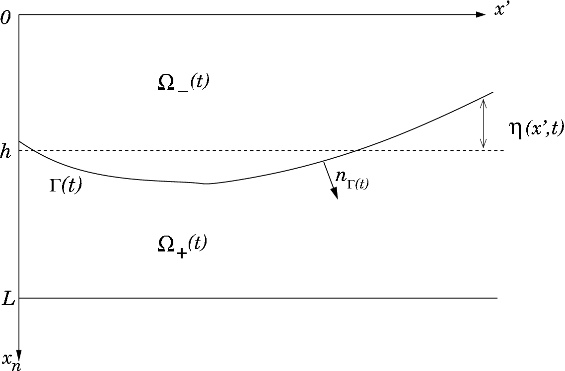
Let $n\in\mathbb{N}$ , $n\geq 2$ , and let $\mathbb{T}^{n-1}:=\mathbb{R}^{n-1}/\mathbb{Z}^{n-1}$ be the $(n-1)$ -dimensional torus. We assume that the porous medium occupies a layer domain $\Omega:=\mathbb{T}^{n-1}\times(0,L)$ , with the $n$ -th unit vector oriented “downwards”, i.e. in the direction of gravity. The domain is separated in two phases by an interface depending on time $t\in[0,T]$ :

$\displaystyle\Omega$	$\displaystyle=$	$\displaystyle\Omega_{-}(t)\cup\Gamma(t)\cup\Omega_{+}(t),$
$\displaystyle\Omega_{-}(t)$	$\displaystyle:=$	$\displaystyle\{(x^{\prime},x_{n})\,\|\,x^{\prime}\in\mathbb{T}^{n-1},\;0<x_{n}<h+\eta(x^{\prime},t)\},$
$\displaystyle\Gamma(t)$	$\displaystyle:=$	$\displaystyle\{(x^{\prime},x_{n})\,\|\,x^{\prime}\in\mathbb{T}^{n-1},x_{n}=h+\eta(x^{\prime},t)\},$
$\displaystyle\Omega_{+}(t)$	$\displaystyle:=$	$\displaystyle\{(x^{\prime},x_{n})\,\|\,x^{\prime}\in\mathbb{T}^{n-1},\;h+\eta(x^{\prime},t)<x_{n}<L\},$

where $h\in(0,L)$ is a fixed reference level and $\eta\in C(\mathbb{R}^{n-1}\times[0,T])$ is such that $h+\eta(x^{\prime},t)\in(0,L)$ for all $(x^{\prime},t)\in\mathbb{R}^{n-1}\times[0,T])$ (cf. Fig. 1.)

Refer to caption — Figure 1: Geometric setting. Note that the $x_{n}$ axis is oriented downwards, and that the liquid phase lies above the vapor phase.

Following [6, 7], we consider the situation in which the upper phase $\Omega_{-}(t)$ is saturated by water under hydrodynamic pressure $P$ while in the lower phase $\Omega_{+}(t)$ the pores of the medium are filled by a vapor-air mixture. This mixture is charaterized by its humidity function $\nu$ given by

\nu=\frac{\rho_{v}}{\rho_{v}+\rho_{a}}\approx\frac{\rho_{v}}{\rho_{a}},

where $\rho_{v}$ and $\rho_{a}$ are the (variable) density of vapor and the (constant) density of air, respectively. The temperature of the mixture and its pressure $P_{a}$ at the interface are assumed constant in time and space. The bulk equations are given just by Darcy’s law with gravity, incompressibility of water, and constant porosity $m$ of the medium, and linear vapor diffusion. Boundary conditions on $\Gamma(t)$ express the pressure balance and fixed evaporation/condensation humidity $\nu^{\ast}$ . A further condition on $\Gamma(t)$ determines its motion from the mass flux balance of water in liquid or vapor form across the phase boundary. From this we get the complete system [7]

\left.\begin{array}[]{rcll}\Delta P&=&0&\mbox{ in $\Omega_{-}(t)$,}\\ (\partial_{t}-D\Delta)\nu&=&0&\mbox{ in $\Omega_{+}(t)$,}\\ \displaystyle\left(1-\frac{\rho_{v}}{\rho_{w}}\right)V_{n}&=&\displaystyle-\frac{k}{m\mu_{w}}\partial_{n_{\Gamma}(t)}(P-\rho_{w}gz)+D\frac{\rho_{a}}{\rho_{w}}\partial_{n_{\Gamma}(t)}\nu&\mbox{ on $\Gamma(t)$,}\\ \nu&=&\nu^{\ast}&\mbox{ on $\Gamma(t)$,}\\ P&=&P_{a}+P_{c}&\mbox{ on $\Gamma(t)$,}\\ P&=&P_{0}&\mbox{ on $\Sigma_{-}$,}\\ \nu&=&\nu_{a}&\mbox{ on $\Sigma_{+}$,}\end{array}\right\}

(1.1)

where $\Sigma_{-}:=\{(x^{\prime},0)\,|\,x^{\prime}\in\mathbb{T}^{n-1}\}$ , $\Sigma_{+}:=\{(x^{\prime},L)\,|\,x^{\prime}\in\mathbb{T}^{n-1}\}$ , $V_{n}$ is the normal velocity of $\Gamma(t)$ , taken positive if $\Omega_{-}(t)$ is expanding, and $n_{\Gamma(t)}$ is the unit normal to $\Gamma(t)$ , exterior to $\Omega_{-}(t)$ .

The following additional constants occur:

$m$ :

porosity of the medium ( $m\in(0,1)$ , fraction of free pore space)
$k$ :

its permeability to water,
$\mu_{w}$ :

viscosity of water,
$D$ :

diffusivity of vapor,
$\rho_{w}$ :

density of water,
$g$ :

gravity,
$P_{c}$ :

capillary pressure,
$P_{0}$ :

hydrodynamic pressure at upper boundary,
$\nu_{a}$ :

humidity at lower boundary.

(Observe that $\rho_{v}$ , which is not constant in the bulk, occurs explicitly only at on $\Gamma(t)$ where we have $\rho_{v}=\rho_{a}\nu\ast={\rm const}$ .)

1.2 Nondimensionalization

Substituting $\nu-\nu_{a}\rightarrow\nu$ , $P-P_{0}\rightarrow P$ , we get

\left.\begin{array}[]{rcll}\Delta P&=&0&\mbox{ in $\Omega_{-}(t)$,}\\ (\partial_{t}-D\Delta)\nu&=&0&\mbox{ in $\Omega_{+}(t)$,}\\ \left(1-\frac{\rho_{v}}{\rho_{w}}\right)V_{n}&=&-\frac{k}{m\mu_{w}}\partial_{n_{\Gamma(t)}}(P-\rho_{w}gz)+D\frac{\rho_{a}}{\rho_{w}}\partial_{n_{\Gamma(t)}}\nu&\mbox{ on $\Gamma(t)$,}\\ \nu&=&\nu^{\ast}-\nu_{a}&\mbox{ on $\Gamma(t)$,}\\ P&=&P_{a}+P_{c}-P_{0}&\mbox{ on $\Gamma(t)$,}\\ P&=&0&\mbox{ on $\Sigma_{-}$,}\\ \nu&=&0&\mbox{ on $\Sigma_{+}$.}\end{array}\right\}

(1.2)

We choose $L$ as characteristic length. The characteristic time $T$ and mass $M$ are defined in view of (1.2)₃, (1.2)₅, from a characteristic pressure and velocity

\frac{M}{LT^{2}}=\rho_{w}gL,\quad\frac{L}{T}=\frac{k\rho_{w}g}{m\mu_{w}}.

This yields the dimensionless formulation

\left.\begin{array}[]{rcll}\Delta P&=&0&\mbox{ in $\Omega_{-}(t)$,}\\ (\partial_{t}-\gamma\Delta)\nu&=&0&\mbox{ in $\Omega_{+}(t)$,}\\ \left(1-\frac{\rho_{v}}{\rho_{w}}\right)V_{n}&=&-\partial_{n_{\Gamma(t)}}P+n_{\gamma}\cdot e_{z}+\frac{\beta}{\nu^{\ast}-\nu_{a}}\partial_{n_{\Gamma(t)}}\nu&\mbox{ on $\Gamma(t)$,}\\ \nu&=&\nu^{\ast}-\nu_{a}&\mbox{ on $\Gamma(t)$,}\\ P&=&\alpha&\mbox{ on $\Gamma(t)$,}\\ P&=&0&\mbox{ on $\Sigma_{-}$,}\\ \nu&=&0&\mbox{ on $\Sigma_{+}$}\end{array}\right\}

(1.3)

with the dimensionless numbers [7]

\alpha=\frac{P_{a}+P_{c}-P_{0}}{\rho_{w}gL},\quad\beta=\frac{D\rho_{a}(\nu^{\ast}-\nu_{a})m\mu_{w}}{k\rho_{w}^{2}gL},\quad\gamma=\frac{DT}{L^{2}}=\frac{Dm\mu_{w}}{k\rho_{w}gL},

see [7] for a physical interpretation of $\alpha$ and $\beta$ . Denoting the scaled function $\eta$ and the scaled region $\Omega$ by the same symbols, the moving interface is now described by

\Gamma(t)=\{(x^{\prime},H+\eta(x^{\prime},t))\}\subset\mathbb{T}^{n-1}\times(0,1),\qquad H=h/L\in(0,1),

(1.4)

the moving domains are

\Omega_{-}(t)=\{(x^{\prime},x_{n})\,|\;0<x_{n}<H+\eta(x^{\prime},t)\},\quad\Omega_{+}(t)=\{(x^{\prime},x_{n})\,|\;H+\eta(x^{\prime},t)<x_{n}<1\},

enclosed by the fixed hyperplanes

\Sigma_{-}=\{(x^{\prime},0)\},\qquad\Sigma_{+}=\{(x^{\prime},1)\}

and subject to

\Omega_{+}(t)\cup\Omega_{-}(t)\cup\Gamma(t)=\Omega=\mathbb{T}^{n-1}\times(0,1).

Normalizing again $\frac{P}{\alpha}\rightarrow P$ , $\frac{\nu}{\nu^{\ast}-\nu_{a}}\rightarrow\nu$ and scaling once more in the time variable finally leads to the system

\left.\begin{array}[]{rcll}\Delta P&=&0&\mbox{ in $\Omega_{-}(t)$,}\\ (\partial_{t}-\Delta)\nu&=&0&\mbox{ in $\Omega_{+}(t)$,}\\ \mu V_{n}&=&-\alpha\partial_{n_{\Gamma(t)}}P+n_{\Gamma(t)}\cdot e_{z}+\beta\partial_{n_{\Gamma(t)}}\nu&\mbox{ on $\Gamma(t)$,}\\ \nu&=&1&\mbox{ on $\Gamma(t)$,}\\ P&=&1&\mbox{ on $\Gamma(t)$,}\\ P&=&0&\mbox{ on $\Sigma_{-}$,}\\ \nu&=&0&\mbox{ on $\Sigma_{+}$,}\end{array}\right\}

(1.5)

which we complement by the initial conditions

\eta(\cdot,0)=\eta_{0}\mbox{ on $\mathbb{T}^{n-1}$},\quad\nu(\cdot,0)=\nu_{0}\mbox{ in $\Omega_{+}(0)$}.

Moreover, we impose the well-posedness condition

\mu\partial_{n_{\Gamma(0)}}\big[\beta\nu_{0}+\alpha P|_{t=0}\big]\leq-\omega_{0}<0\mbox{ on }\Gamma(0).

(1.6)

Observe that this is in fact a demand on $\eta_{0}$ and $\nu_{0}$ only. For later use we collect the facts that

\partial_{n_{\Gamma(t)}}=\frac{1}{\sqrt{1+|\nabla_{x}\eta|^{2}}}(-\nabla_{x}\eta\cdot\nabla_{x}+\partial_{z}),\quad V_{n}=\frac{\partial_{t}\eta}{\sqrt{1+|\nabla_{x}\eta|^{2}}}

and that (1.5)₃ takes the form

\mu\partial_{t}\eta=(-\nabla_{x}\eta\cdot\nabla_{x}+\partial_{z})(-\alpha P+\beta\nu)+1\quad\mbox{ on $\Gamma(t)$.}

2 Transformation

Following a standard approach we aim to transform system (1.5) to a fixed reference geometry. Oriented at [12] we define

\displaystyle\Omega_{-}:=\{(x^{\prime},x_{n})\,|\,x_{n}\in(0,H)\},\quad\Omega_{+}:=\{(x^{\prime},x_{n})\,|\,x_{n}\in(H,1)\},\quad\Gamma:=\{(x^{\prime},H)\},

and consider continuous functions $\hat{\phi}:\Omega\times[0,T]\longrightarrow\mathbb{R}$ such that

\hat{\phi}(\cdot,t)=0\quad\mbox{ on $\Sigma_{\pm}$},\quad\hat{\phi}((z^{\prime},H),t)=\eta(z^{\prime},t),\quad t\in[0,T],

(2.1)

$\hat{\phi}|_{\Omega_{\pm}}$ and $\hat{\phi}|_{\Gamma}$ are sufficiently smooth, and

z\mapsto(z^{\prime},z_{n}+\hat{\phi}(z,t))\in{\rm Diff}(\Omega_{\pm},\Omega_{\pm}(t)),\quad t\in[0,T].

(2.2)

(The function $\hat{\phi}$ we are going to construct in the following will satisfy these demands, see Lemma 2.2, Eqns. (2.9), (2.17) and Theorem 2.5 below.) Denote the inverse of the mapping (2.2) by $Z_{\hat{\phi}}(\cdot,t)$ and define

	$\displaystyle\hat{P}(z,t)$	$\displaystyle=$	$\displaystyle P(Z_{\hat{\phi}}^{-1}(z,t),t),\quad z\in\Omega_{-},$		(2.3)
	$\displaystyle\hat{\nu}(z,t)$	$\displaystyle=$	$\displaystyle\nu(Z_{\hat{\phi}}^{-1}(z,t),t),\quad z\in\Omega_{+}.$		(2.4)

Then system (1.5) is transformed to

\left.\begin{array}[]{rcll}\displaystyle{\cal A}_{\hat{\phi}}\hat{P}-\frac{\hat{P}_{z_{n}}}{1+{\hat{\phi}}_{z_{n}}}{\cal A}_{\hat{\phi}}{\hat{\phi}}&=&0&\mbox{ in $\Omega_{-}\times J$,}\\ \displaystyle L_{\hat{\phi}}\hat{\nu}-\frac{\hat{\nu}_{z_{n}}}{1+{\hat{\phi}}_{z_{n}}}L_{\hat{\phi}}{\hat{\phi}}&=&0&\mbox{ in $\Omega_{+}\times J$,}\\ \mu\partial_{t}{\hat{\phi}}&=&\displaystyle(1+|\nabla^{\prime}{\hat{\phi}}|^{2})\left(\frac{-\alpha\hat{P}_{z_{n}}}{1+{\hat{\phi}}^{-}_{z_{n}}}+\frac{\beta\hat{\nu}_{z_{n}}}{1+{\hat{\phi}}^{+}_{z_{n}}}\right)+1&\mbox{ on $\Gamma\times J$,}\\ \hat{\nu}&=&1&\mbox{ on $\Gamma\times J$,}\\ \hat{P}&=&1&\mbox{ on $\Gamma\times J$,}\\ \hat{P}&=&0&\mbox{ on $\Sigma_{-}\times J$,}\\ \hat{\nu}&=&0&\mbox{ on $\Sigma_{+}\times J$,}\\ \hat{\nu}(\cdot,0)&=&\hat{\nu}_{0}:=\nu_{0}\circ Z^{-1}_{{\hat{\phi}}}(\cdot,0)&\mbox{ in $\Omega_{+}$,}\\ {\hat{\phi}}(\cdot,0)&=&\eta_{0}&\mbox{ on $\Gamma$,}\end{array}\right\}

(2.5)

where

$\displaystyle L_{\hat{\phi}}u$	$\displaystyle:=$	$\displaystyle\partial_{t}u-{\cal A}_{\hat{\phi}}u,$
$\displaystyle{\cal A}_{\hat{\phi}}u$	$\displaystyle:=$	$\displaystyle\sum_{i=1}^{n-1}u_{z_{i}z_{i}}-\vec{a}(\nabla{\hat{\phi}})\cdot\nabla u_{z_{n}},$
$\displaystyle\vec{a}(\nabla{\hat{\phi}})$	$\displaystyle:=$	$\displaystyle\left(\frac{2\nabla^{\prime}{\hat{\phi}}}{1+{\hat{\phi}}_{z_{n}}},-\frac{1+\|\nabla^{\prime}{\hat{\phi}}\|^{2}}{(1+{\hat{\phi}}_{z_{n}})^{2}}\right)$

(Observe that we will assume continuity but not differentiability of ${\hat{\phi}}$ across $\Gamma$ and therefore have to distinguish one-sided derivatives ${\hat{\phi}}^{\pm}_{z_{n}}$ on $\Gamma$ ).

Before we can start to discuss system (2.5) we have to introduce some notation and make some general assumptions which we keep fixed afterwards:

Let $\mathbb{H}^{n}_{\pm}:=\{(x^{\prime},x_{n})\,|\,x^{\prime}\in\mathbb{R}^{n-1},\,x_{n}\gtrless H\}$ , $\mathbb{R}^{n}_{\pm}:=\{(x^{\prime},x_{n})\,|\,x^{\prime}\in\mathbb{R}^{n-1},\,x_{n}\gtrless 0\}$ .

For $s\geq 0$ and a Banach space $Y$ , $M\in\{\Omega_{\pm},\Gamma,\mathbb{R}^{n}_{\pm},\mathbb{H}^{n}_{\pm},[0,T]\}$ ( $T>0$ ) we denote by $H_{p}^{s}(M,Y)$ the Bessel potential space and by $W_{p}^{s}(M,Y)$ the $L^{p}$ -based Sobolev space of order $s$ . In particular, if $s\notin\mathbb{N}$ , this fractional-order Sobolev space coincides with the Besov space $B_{pp}^{s}(M,Y)$ , and for $s\in\mathbb{N}$ the we have $W_{p}^{s}(M,Y)=H_{p}^{s}(M,Y)$ (cf. [13]). For the sake of brevity we write $W_{p}^{s}(M):=W_{p}^{s}(M,\mathbb{R})$ .

Finally, here and in the following we assume that $p>n+3/2+\sqrt{2n+1/4}$ and that

\eta_{0}\in W_{p}^{2-2/p}(\Gamma),\quad\eta_{0}(x^{\prime})\in(\gamma-H,1-\gamma-H)\quad\mbox{for some }\gamma>0.

For technical reasons it is convenient to reduce system (2.5) to the case of homogeneous initial data. For this we need the following two lemmas:

Lemma 2.1

There is a linear extension operator $T\in{\cal L}(W_{p}^{2-1/p}(\Gamma\times\mathbb{R}),H^{2}_{p}(\Omega\times\mathbb{R}))$ with the properties

Tg|_{\Gamma\times\mathbb{R}}=g,\quad\partial_{n}Tg|_{\Gamma\times\mathbb{R}}=0,\qquad g\in W_{p}^{2-1/p}(\Gamma\times\mathbb{R}).

Proof: Define first $T^{-}\in{\cal L}(W_{p}^{2-1/p}(\Gamma\times\mathbb{R}),H^{2}_{p}(\Omega_{-}\times\mathbb{R}))$ by setting (for example) $T^{-}g:=u$ where $u$ solves the elliptic fourth order problem

\Delta^{2}u=0\quad\mbox{in $\Omega_{-}\times\mathbb{R}$},\quad u|_{\Gamma\times\mathbb{R}}=g,\quad u_{z_{n}}|_{\Gamma\times\mathbb{R}}=0,\quad u|_{\Sigma_{-}\times\mathbb{R}}=0,\quad u_{z_{n}}|_{\Sigma_{-}\times\mathbb{R}}=0.

Then construct $T$ by extension using [13] Theorem 3.3.4.

Lemma 2.2

There is a time interval $J=(0,\tau)$ and $\sigma\in H^{2}_{p}(\Omega\times J)$ such that

\sigma|_{\Gamma\times\{0\}}=\eta_{0},\quad\sigma|_{\Sigma_{\pm}\times J}=0.

(2.6)

Moreover, the mapping $\psi(\cdot,t):=[(z^{\prime},z_{n})\mapsto(z^{\prime},z_{n}+\sigma(z,t))]$ is for each $t\in\bar{J}$ a diffeomorphism onto its image satisfying

\inf_{t\in J}\det D\psi(\cdot,t)\geq\delta>0

The numbers $\tau$ , $\|\sigma\|_{H^{2}_{p}(\Omega\times J)}$ , and $\delta$ depend only on $\|\eta_{0}\|_{W_{p}^{2-2/p}(\Gamma)}$ and $\gamma$ .

Proof: Define $\eta_{1}\in W_{p}^{2-1/p}(\Gamma\times\mathbb{R}_{+})$ as solution $u$ to the standard BVP

\Delta u=0\quad\mbox{in $\Gamma\times\mathbb{R}_{+}$,}\quad u|_{\Gamma\times\{0\}}=\eta_{0}.

Extend $\eta_{1}$ to $\eta_{2}\in W_{p}^{2-1/p}(\Gamma\times\mathbb{R})$ by [13] Theorem 2.9.4 and Proposition 2.9.1.2. Let $h:=\eta_{2}+H\in W_{p}^{2-1/p}(\Gamma\times\mathbb{R})$ . Let $T$ be the operator from Lemma 2.1. As $Th$ has Hölder continuous derivatives there are $\eta^{-}\in(H-\gamma/4,H)$ , $\eta^{+}\in(H,H+\gamma/4)$ , $\tau>0$ , such that

Th(z,t)>\frac{3}{4}\gamma,\quad\partial_{n}Th(z,t)>-\frac{1}{2}\qquad\mbox{for $z_{n}\in(\eta^{-},H)$, $t\in[0,\tau]$},

(2.7)

Th(z,t)<1-\frac{3}{4}\gamma,\quad\partial_{n}Th(z,t)>-\frac{1}{2}\qquad\mbox{for $z_{n}\in(H,\eta^{+})$, $t\in[0,\tau]$}.

(2.8)

Let $\chi\in C^{\infty}_{0}(0,1)$ be such that $\mathop{\rm supp}\chi\in(\eta^{-},\eta^{+})$ , $\chi(y)\equiv 1$ near $y=H$ , $\chi^{\prime}\geq 0$ on $(0,H)$ , and $\chi^{\prime}\leq 0$ on $(H,1)$ .

Define $\psi_{n}$ by

\psi_{n}(z,t):=\left\{\begin{array}[]{rl}\displaystyle(1-\chi(z_{n}))\frac{\gamma}{4}z_{n}+\chi(z_{n})(z_{n}-H+Th(z,t)),&\ z\in\Omega_{-},\\ \displaystyle(1-\chi(z_{n}))(1+\frac{\gamma}{4}(z_{n}-1))+\chi(z_{n})(z_{n}-H+Th(z,t)),&\ z\in\Omega_{+}\\ \end{array}\right.

and let

\psi(z,t):=(z^{\prime},\psi_{n}(z,t)).

Then

\psi(z^{\prime},0,t)=0,\quad\psi(z^{\prime},1,t)=1,\quad\psi(z^{\prime},H,t)=h,\quad\partial_{n}\psi(z^{\prime},H,t)=1,\qquad t\in J,

and to prove the lemma it remains to show that $\partial_{n}\psi_{n}\geq\delta>0$ on $\Omega$ . This is clear for $z_{n}\in[0,\eta^{-}]$ and $z_{n}\in[\eta^{+},1]$ . For $z_{n}\in[\eta^{-},H]$ we recall $\chi^{\prime}(z_{n})\geq 0$ , $z_{n}-H>-\gamma/4$ , and (2.7) and conclude

			$\displaystyle\partial_{n}\psi_{n}(z,t)=(1-\chi(z_{n}))\frac{\gamma}{4}+\chi(z_{n})(1+\partial_{n}Th(z,t))$
			$\displaystyle+\chi^{\prime}(z_{n})(z_{n}-H+Th(z,t)-\frac{\gamma}{4}z_{n})$
		$\displaystyle\geq$	$\displaystyle\min(\gamma/4,1/2).$

Similarly, for $z_{n}\in[H,\eta^{+}]$ , we have $\chi^{\prime}(z_{n})\leq 0$ , $z_{n}-H<\gamma/4$ , and conclude from this and (2.8)

			$\displaystyle\partial_{n}\psi_{n}(z,t)=(1-\chi(z_{n}))\frac{\gamma}{4}+\chi(z_{n})(1+\partial_{n}Th(z,t))$
			$\displaystyle+\chi^{\prime}(z_{n})(z_{n}-H+Th(z,t)-1-\frac{\gamma}{4}(z_{n}-1))$
		$\displaystyle\geq$	$\displaystyle\min(\gamma/4,1/2).$

The proof is completed by setting $\sigma(z,t):=\psi_{n}(z,t)-z_{n}$ .

Remark 2.3

For later use we emphasize the fact that for each $\rho\in(0,1)$ we have

\sigma\in W_{p}^{\rho}((0,\tau),W_{p}^{2-\rho}(\Omega))

cf. Lemma 4.3 in [3].

Set

\quad{\hat{\phi}}:=\sigma+\phi,\quad\hat{P}:=Q+p,\quad\hat{\nu}=V+v,

(2.9)

where $Q$ satisfies the (time-) parameter dependent family of elliptic BVPs

\left.\begin{array}[]{rcll}\displaystyle{\cal A}_{\sigma}Q-\frac{Q_{z_{n}}}{1+\sigma_{z_{n}}}{\cal A}_{\sigma}\sigma&=&0&\mbox{ in $\Omega_{-}\times J$,}\\ Q&=&1&\mbox{ on $\Gamma\times J$,}\\ Q&=&0&\mbox{ on $\Sigma_{-}\times J$,}\end{array}\right\}

(2.10)

and $V$ satisfies the parabolic IBVP

\left.\begin{array}[]{rcll}\displaystyle L_{\sigma}V-\frac{V_{z_{n}}}{1+\sigma_{z_{n}}}L_{\sigma}\sigma&=&0&\mbox{ in $\Omega_{+}\times J$,}\\ V&=&1&\mbox{ on $\Gamma\times J$,}\\ V&=&0&\mbox{ on $\Sigma_{+}\times J$,}\\ V(\cdot,0)&=&\hat{\nu}_{0}&\mbox{ in $\Omega_{+}$.}\end{array}\right\}

(2.11)

The functions $Q$ and $V$ are easily seen to be well defined:

Lemma 2.4

Let $\theta\in\left(\frac{1}{p}\,\frac{p-1}{p-n},\frac{1}{2}\left(1-\frac{n+1}{p}\right)\right)$ and assume $\hat{\nu}_{0}\in W_{p}^{2-2/p}(\Omega_{+})$ . For some $T\in(0,\tau)$ the problems (2.10) and (2.11) possess unique solutions $Q\in L_{p}(0,T;W_{p}^{2}(\Omega_{-}))\cap W_{p}^{\theta}((0,T),W_{p}^{2-\theta}(\Omega_{-}))$ and $V\in L_{p}(0,T;W_{p}^{2}(\Omega_{+}))\cap H_{p}^{1}((0,T);L_{p}(\Omega_{+}))$ .

Proof: By construction $1+\sigma_{z_{n}}$ is invertible in the Banach algebra $H_{p}^{1}((0,\tau)\times\Omega)$ and by embedding in the algebras $W_{p}^{\theta}((0,\tau),W_{p}^{1-\theta}(\Omega_{-}))$ , $L_{\infty}((0,\tau),W_{p}^{1-\theta}(\Omega_{-}))$ and $L_{\infty}((0,\tau)\times\Omega_{+})$ , too. The assertion is a consequence of the regularity of $\sigma$ , Lemma A.4, and (a periodic version of) known parabolic theory [8].

We divide equation $\mbox{(\ref{mbp5})}_{(3)}$ by $\mu\neq 0$ and use the same symbols $\alpha$ , $\beta$ again instead of $\alpha/\mu$ , $\beta/\mu$ . This turns Condition (1.6) into

\partial_{n_{\Gamma(0)}}\big[\beta\nu_{0}+\alpha P|_{t=0}\big]\leq-\omega_{0}<0\mbox{ on }\Gamma(0).

(2.12)

In view of Lemma 2.4 the problem (2.5) is reduced to finding $\phi,p,v$ from the (formal) system

F(\sigma+\phi,Q+p,V+v)=0,

(2.13)

where

F(\tau,q,w):=\left(\begin{array}[]{c}\displaystyle{\cal A}_{\tau}q-\frac{q_{z_{n}}}{1+\tau_{z_{n}}}{\cal A}_{\tau}\tau\\ \displaystyle L_{\tau}w-\frac{w_{z_{n}}}{1+\tau_{z_{n}}}L_{\tau}\tau\\ \displaystyle\left.\left(\partial_{t}\tau-(1+|\nabla^{\prime}\tau|^{2})\left(\frac{-\alpha q_{z_{n}}}{1+\tau^{-}_{z_{n}}}+\frac{\beta w_{z_{n}}}{1+\tau^{+}_{z_{n}}}\right)\right)\right|_{\Gamma}-1/\mu\\ q|_{\Gamma}-1\\ w|_{\Gamma}-1\\ q|_{\Sigma_{-}}\\ w|_{\Sigma_{+}}\end{array}\right)

(2.14)

complemented by the given initial conditions. Furthermore, our choices for $\phi$ will ensure that $(\phi,p,v)$ vanishes at $t=0$ and is therefore small in suitable norms for short times. Terms that are quadratic in this triple will therefore be treated as small perturbations to the linearized problem.

Rewrite (2.13) equivalently as

F^{\prime}(\sigma,Q,V)[\phi,p,v]=-F(\sigma,Q,V)-R,

(2.15)

where

$\displaystyle R$	$\displaystyle=$	$\displaystyle\int_{0}^{1}(1-s)\frac{d^{2}}{ds^{2}}[F((\sigma,Q,V)+s(\phi,p,v))]\,ds$
	$\displaystyle=$	$\displaystyle\int_{0}^{1}(1-s)F^{\prime\prime}((\sigma,Q,V)+s(\phi,p,v))[(\phi,p,v),(\phi,p,v)]\,ds$
	$\displaystyle=:$	$\displaystyle(R_{1},R_{2},R_{3},0,0,0,0).$

Observe, in particular,

\partial_{\tau}{\cal A}_{\sigma}w[\phi]=-A(\nabla\sigma)\nabla\phi\cdot\nabla w_{z_{n}},\quad A(p):=D_{p}\vec{a}(p)

(2.16)

From now on, for the sake of convenience we will write $\phi^{\pm}$ for the restrictions of $\phi$ to $\Omega_{\pm}$ and retain the notation $\phi$ for the trace at $\Gamma$ . The demands $(\ref{phihat})$ and $(\ref{demsigma})$ together with the continuity of $\hat{\phi}$ across $\Gamma$ imply

\left.\begin{array}[]{rcll}\phi^{\pm}-\phi&=&0&\mbox{ on $\Gamma\times J$,}\\ \phi^{\pm}&=&0&\mbox{ on $\Sigma_{\pm}\times J$,}\\ \phi(\cdot,0)&=&0&\mbox{ on $\Gamma$.}\end{array}\right\}

(2.17)

Additionally, it will be convenient to write $Q=:U^{-}$ , $V=:U^{+}$ , $p=u^{-}$ , $v=u^{+}$ ${\cal A}_{\sigma}=:\Lambda_{\sigma}^{-}$ , $L_{\sigma}=:\Lambda_{\sigma}^{+}$ . Then (2.15) takes the form

\left.\begin{array}[]{rcll}\tilde{L}^{\pm}u^{\pm}-\frac{U^{\pm}_{z_{n}}}{1+\sigma_{z_{n}}}L^{\pm}\phi^{\pm}&=&K^{\pm}\phi^{\pm}+R^{\pm}(\phi^{\pm},u^{\pm})&\mbox{ in $\Omega_{\pm}\times J$,}\\[4.30554pt] \partial_{t}\phi-\alpha^{-}\phi^{-}_{z_{n}}-\alpha^{+}\phi^{+}_{z_{n}}&&&\\ +\zeta\cdot\nabla^{\prime}\phi-\tilde{\alpha}^{-}u^{-}_{z_{n}}-\tilde{\alpha}^{+}u^{+}_{z_{n}}&=&g_{0}+R^{B}(\phi^{-}\phi^{+},\phi,u^{-},u^{+})&\mbox{ on $\Gamma\times J$},\\[4.30554pt] u^{\pm}&=&0&\mbox{ on $\Sigma_{\pm}\times J$},\\ u^{+}(\cdot,0)&=&0&\mbox{ in $\Omega_{0}$,}\end{array}\right\}

(2.18)

where

$\displaystyle L^{\pm}\phi^{\pm}$	$\displaystyle:=$	$\displaystyle\Lambda_{\sigma}^{\pm}\phi^{\pm}\pm A(\nabla\sigma)\nabla\phi^{\pm}\cdot\nabla\sigma_{z_{n}},$
$\displaystyle\tilde{L}^{\pm}u^{\pm}$	$\displaystyle:=$	$\displaystyle\Lambda_{\sigma}^{\pm}u^{\pm}-\frac{u^{\pm}_{z_{n}}}{1+\sigma_{z_{n}}}\Lambda_{\sigma}\sigma,$
$\displaystyle K^{\pm}\phi^{\pm}$	$\displaystyle:=$	$\displaystyle A(\nabla\sigma)\nabla\phi^{\pm}\cdot\nabla U^{\pm}_{z_{n}}-\frac{U^{\pm}_{z_{n}}}{(1+\sigma_{z_{n}})^{2}}\phi^{\pm}_{z_{n}}\Lambda_{\sigma}\sigma,$

$\displaystyle\alpha^{-}$	$\displaystyle:=\alpha\frac{U^{-}_{z_{n}}(1+\|\nabla^{\prime}\sigma\|^{2})}{(1+\sigma_{z_{n}})^{2}},$	$\displaystyle\alpha^{+}$	$\displaystyle:=-\beta\frac{U^{+}_{z_{n}}(1+\|\nabla^{\prime}\sigma\|^{2})}{(1+\sigma_{z_{n}})^{2}},$
$\displaystyle\tilde{\alpha}^{-}$	$\displaystyle:=-\alpha\frac{1+\|\nabla^{\prime}\sigma\|^{2}}{1+\sigma_{z_{n}}},$	$\displaystyle\tilde{\alpha}^{+}$	$\displaystyle:=\beta\frac{1+\|\nabla^{\prime}\sigma\|^{2}}{1+\sigma_{z_{n}}},$
$\displaystyle\zeta$	$\displaystyle:=\frac{2(\alpha U^{-}_{z_{n}}-\beta U^{+}_{z_{n}})}{1+\sigma_{z_{n}}}\nabla^{\prime}\sigma,$

g_{0}:=1/\mu-\partial_{t}\sigma+\frac{1+|\nabla^{\prime}\sigma|^{2}}{1+\sigma_{z_{n}}}(-\alpha U^{-}_{z_{n}}+\beta U^{+}_{z_{n}}),

			$\displaystyle R^{B}(\phi^{-},\phi^{+},\phi,u^{-},u^{+})$
		$\displaystyle:=$	$\displaystyle(1+\|\nabla^{\prime}\sigma\|^{2})\left(\alpha\left(\frac{u_{z_{n}}^{-}\phi_{z_{n}}^{-}}{(1+\sigma_{z_{n}})(1+\sigma_{z_{n}}+\phi^{-}_{z_{n}})}-\frac{U^{-}_{z_{n}}{\phi^{-}_{z_{n}}}^{2}}{(1+\sigma_{z_{n}})^{2}(1+\sigma_{z_{n}}+\phi^{-}_{z_{n}})}\right)\right.$
			$\displaystyle\left.-\beta\left(\frac{u_{z_{n}}^{+}\phi_{z_{n}}^{+}}{(1+\sigma_{z_{n}})(1+\sigma_{z_{n}}+\phi^{+}_{z_{n}})}-\frac{U^{+}_{z_{n}}{\phi^{+}_{z_{n}}}^{2}}{(1+\sigma_{z_{n}})^{2}(1+\sigma_{z_{n}}+\phi^{+}_{z_{n}})}\right)\right)$
			$\displaystyle+2\nabla^{\prime}\sigma\cdot\nabla^{\prime}\phi\left(-\alpha\left(\frac{u_{z_{n}}^{-}}{1+\sigma_{z_{n}}+\phi^{-}_{z_{n}}}-\frac{U_{z_{n}}^{-}\phi_{z_{n}}^{-}}{(1+\sigma_{z_{n}})(1+\sigma_{z_{n}}+\phi^{-}_{z_{n}})}\right)\right.$
			$\displaystyle\left.+\beta\left(\frac{u_{z_{n}}^{+}}{1+\sigma_{z_{n}}+\phi^{+}_{z_{n}}}-\frac{U_{z_{n}}^{+}\phi_{z_{n}}^{+}}{(1+\sigma_{z_{n}})(1+\sigma_{z_{n}}+\phi^{+}_{z_{n}})}\right)\right)$
			$\displaystyle+\|\nabla^{\prime}\phi\|^{2}\left(-\alpha\frac{U_{z_{n}}^{-}+u_{z_{n}}^{-}}{1+\sigma_{z_{n}}+\phi^{-}_{z_{n}}}+\beta\frac{U_{z_{n}}^{+}+u_{z_{n}}^{+}}{1+\sigma_{z_{n}}+\phi^{+}_{z_{n}}}\right),$

and

			$\displaystyle R_{\pm}(\phi^{\pm},u^{\pm})$
		$\displaystyle:=$	$\displaystyle A(\nabla\sigma)\nabla\phi^{\pm}\nabla u^{\pm}_{z_{n}}+\vec{b}(\nabla\sigma,\nabla\phi^{\pm})(\nabla U^{\pm}_{z_{n}}+\nabla u^{\pm}_{z_{n}})$
			$\displaystyle+\frac{U^{\pm}_{z_{n}}+u^{\pm}_{z_{n}}}{1+\sigma_{z_{n}}+\phi^{\pm}_{z_{n}}}\big(A(\nabla\sigma)\nabla\phi^{\pm}\nabla\phi^{\pm}_{z_{n}}+\vec{b}(\nabla\sigma,\nabla\phi^{\pm})(\nabla\sigma_{z_{n}}+\nabla\phi^{\pm}_{z_{n}})\big)$
			$\displaystyle+\frac{\phi^{\pm}_{z_{n}}L^{\pm}_{\sigma}\sigma}{(1+\sigma_{z_{n}})(1+\sigma_{z_{n}}+\phi^{\pm}_{z_{n}})}(u^{\pm}_{z_{n}}-\frac{U^{\pm}_{z_{n}}\phi^{\pm}_{z_{n}}}{1+\sigma_{z_{n}}}),$

where

\vec{b}(\nabla\sigma,\nabla\phi^{\pm}):=\sum_{i=0}^{n}\int_{0}^{1}(1-s)\partial_{i}A(\nabla\sigma+s\nabla\phi^{\pm})\partial_{i}\phi^{\pm}\cdot\nabla\phi^{\pm}\;ds.

To simplify the equations we use the remaining freedom of choice for $\phi$ to demand

L^{\pm}\phi^{\pm}=0\quad\mbox{ in $\Omega_{\pm}\times J$,}\qquad\phi^{+}(\cdot,0)=0\quad\mbox{ in $\Omega_{+}$.}

(2.19)

Together with (2.17) the demands yield a uniquely solvable time dependent elliptic boundary value problem for $\phi^{-}$ and a uniquely solvable initial boundary value problem for $\phi^{+}$ that determine $\phi^{\pm}$ completely in terms of $\phi$ . In particular, we have $\phi^{-}(\cdot,0)=0$ in $\Omega_{-}$ , and therefore $\sigma={\hat{\phi}}$ at $t=0$ . Comparing now (2.5)_1,5,6 to (2.10) at $t=0$ shows $\hat{P}(\cdot,0)=Q(\cdot,0)$ in $\Omega_{-}$ , and thus also $p(\cdot,0)=u^{-}(\cdot,0)=0$ .

The following theorem is the main result of this paper:

Theorem 2.5

Let $p$ be as specified above, $\theta\in\left(\frac{1}{p}\,\frac{p-1}{p-n},\frac{1}{2}\left(1-\frac{n+1}{p}\right)\right)$ and assume (2.12). There is a positive time $T_{0}\in(0,\tau)$ such that the nonlinear problem (2.17), (2.18), (2.19) possesses a unique solution

$\displaystyle((u^{+},\phi^{+}),(u^{-},\phi^{-}),\phi)$	$\displaystyle\in$	$\displaystyle\quad\big[L_{p}(0,T_{0};W_{p}^{2}(\Omega_{+}))\cap H_{p}^{1}((0,T_{0});L_{p}(\Omega_{+}))\big]^{2}$
		$\displaystyle\times\;\big[L_{p}(0,T_{0};W_{p}^{2}(\Omega_{-}))\cap W_{p}^{\theta}((0,T_{0}),W_{p}^{2-\theta}(\Omega_{-}))\big]^{2}$
		$\displaystyle\times\;L_{p}(0,T_{0};W_{p}^{2-1/p}(\Gamma))\cap H_{p}^{1}((0,T_{0}),W_{p}^{1-1/p}(\Gamma))$
		$\displaystyle\quad\,\cap\;W^{1+\theta}_{p}((0,T_{0}),L_{p}(\Gamma)).$

Remark 2.6

We briefly sketch how to obtain a solution of problem (1.5) from Theorem 2.5. Define $\tilde{\phi}\in C(\bar{\Omega}\times[0,T_{0}])$ by

\tilde{\phi}=\left\{\begin{array}[]{lcr}\phi^{-}&\mbox{ in }&\Omega_{-}\times[0,T_{0}],\\ \phi^{+}&\mbox{ in }&\Omega_{+}\times[0,T_{0}],\\ \phi&\mbox{ on }&\Gamma\times[0,T_{0}],\end{array}\right.

and let

\hat{\phi}:=\sigma+\tilde{\phi},\qquad\eta:=\hat{\phi}|_{\Gamma\times[0,T_{0}]}.

Defining $P$ and $\nu$ by means of $\hat{P}:=U^{-}+u^{-}$ , $\hat{\nu}:=U^{+}+u^{+}$ and (2.3), (2.4), the triple $(P,\nu,\eta)$ is a solution to (1.5).

Our proof of Theorem 2.5 will rely on a careful study of the linear part of (2.18) which is done in the next section.

3 The linearized problem

3.1 Function spaces and optimal regularity for the full linearized problem

Neglecting lower order terms in (2.18) that will be absorbed on the right side we consider the linear elliptic-parabolic problem with dynamic boundary condition

\left.\begin{array}[]{rcll}\displaystyle\tilde{L}^{\pm}u^{\pm}&=&f^{\pm}&\mbox{ in $\Omega_{\pm}$,}\\ L^{\pm}\phi^{\pm}&=&0&\mbox{ in $\Omega_{\pm}$,}\\ \phi^{\pm}-\phi&=&0&\mbox{ on $\Gamma\times J$,}\\ \phi^{\pm}&=&0&\mbox{ on $\Sigma_{\pm}\times J$,}\\ u^{\pm}&=&0&\mbox{ on $\Gamma\cup\Sigma_{\pm}$},\\ \partial_{t}\phi-\alpha^{-}\phi^{-}_{z_{n}}-\alpha^{+}\phi^{+}_{z_{n}}+\zeta\cdot\nabla^{\prime}\phi-\tilde{\alpha}^{-}u^{-}_{z_{n}}-\tilde{\alpha}^{+}u^{+}_{z_{n}}&=&g&\mbox{ on $\Gamma$},\\ u^{+}(\cdot,0)&=&0&\mbox{ in $\Omega_{+}$,}\\ \phi^{+}(\cdot,0)&=&0&\mbox{ in $\bar{\Omega}_{+}$.}\end{array}\right\}

(3.1)

Here and in the following we assume that

\theta,\theta^{\prime}\in\left(\frac{1}{p}\,\frac{p-1}{p-n},\frac{1}{2}\left(1-\frac{n+1}{p}\right)\right).

With $J:=[0,T]$ ( $T\in(0,\tau)$ ) we further define

•

for $M\in\{\mathbb{R}^{n-1},\mathbb{T}^{n-1},\Gamma\}$ :

$\displaystyle X^{B}(M)$	$\displaystyle:=$	$\displaystyle X_{\theta}^{B}(M)$
	$\displaystyle:=$	$\displaystyle L_{p}(J,W_{p}^{2-1/p}(M))\cap H_{p}^{1}(J,W_{p}^{1-1/p}(M))\cap W^{1+\theta}_{p}(J,L_{p}(M)),$
$\displaystyle Y^{B}(M)$	$\displaystyle:=$	$\displaystyle Y_{\theta}^{B}(M):=L_{p}(J,W_{p}^{1-1/p}(M))\cap W^{\theta}_{p}(J,L_{p}(M)),$
$\displaystyle X_{\mathop{\rm tr}}^{-}(M)$	$\displaystyle:=$	$\displaystyle X_{{\mathop{\rm tr}},\theta}^{-}(M):=L_{p}(J,W_{p}^{2-1/p}(M))\cap W_{p}^{\theta}(J,W^{2-\theta-1/p}_{p}(M)),$

•

for $M\in\{\mathbb{H}^{n}_{+},\Omega_{+},\mathbb{R}^{n}_{+}\}$ :

$\displaystyle X^{+}(M)$	$\displaystyle:=$	$\displaystyle L_{p}(J,H_{p}^{2}(M)\cap H_{p}^{1}(J,L_{p}(M)),$
$\displaystyle Y^{+}(M)$	$\displaystyle:=$	$\displaystyle L_{p}(M\times J),$
$\displaystyle Z^{+}(M)$	$\displaystyle:=$	$\displaystyle L_{p}(J,H_{p}^{1}(M))\cap W_{p}^{1/2}(J,L_{p}(M)),$

•

for $M\in\{\mathbb{H}^{n}_{-},\Omega_{-},\mathbb{R}^{n}_{\pm}\}$ :

$\displaystyle X^{-}(M)$	$\displaystyle:=$	$\displaystyle X_{\theta}^{-}(M):=L_{p}(J,H_{p}^{2}(M))\cap W^{\theta}_{p}(J,W^{2-\theta}_{p}(M)),$
$\displaystyle Y^{-}(M)$	$\displaystyle:=$	$\displaystyle Y_{\theta}^{-}(M):=L_{p}(M\times J)\cap W^{\theta}_{p}(J,W^{-\theta}_{p}(M)),$
$\displaystyle Z^{-}(M)$	$\displaystyle:=$	$\displaystyle Z_{\theta}^{-}(M):=L_{p}(J,H_{p}^{1}(\Omega))\cap W_{p}^{\theta}(J,W_{p}^{1-\theta}(\Omega)),$

•

further:

$\displaystyle X^{+}_{\mathop{\rm tr}}(\Gamma)$	$\displaystyle:=$	$\displaystyle L_{p}(J,W_{p}^{2-1/p}(\Gamma))\cap W_{p}^{1-1/(2p)}(J,L_{p}(\Gamma)),$
$\displaystyle Z^{0}(\Omega)$	$\displaystyle:=$	$\displaystyle L_{p}(J,H_{p}^{1}(\Omega))\cap H_{p}^{1}(J,L_{p}(\Omega)),$
$\displaystyle Z^{+}_{\mathop{\rm tr}}(\Gamma)$	$\displaystyle:=$	$\displaystyle L_{p}(J,W_{p}^{1-1/p}(\Gamma))\cap W_{p}^{(1-1/p)/2}(J,L_{p}(\Gamma)),$
$\displaystyle Z^{-}_{\mathop{\rm tr}}(\Gamma)$	$\displaystyle:=$	$\displaystyle Z^{-}_{{\mathop{\rm tr}},\theta}(\Gamma):=L_{p}(J,W_{p}^{1-1/p}(\Gamma))\cap W_{p}^{\theta}(J,W_{p}^{1-1/p-\theta}(\Gamma)).$

For any space $U$ in this list, let $\underaccent{\circ}{U}$ be the (closed) subspace of $U$ for which the traces $u|_{t=0}$ and $\partial_{t}u|_{t=0}$ vanish in case these traces exist. The main result of this section reads as follows:

Theorem 3.1

Let Let $p>n+3/2+\sqrt{2n+1/4}$ , $\theta,\theta^{\prime}\in\left(\frac{1}{p}\,\frac{p-1}{p-n},\frac{1}{2}\left(1-\frac{n+1}{p}\right)\right)$ and assume (2.12). For some $T_{0}\in(0,\tau)$ and

(f^{+},f^{-},g)\in Y^{+}(\Omega_{+})\times Y_{\theta}^{-}(\Omega_{-})\times Y_{\theta}^{B}(\Gamma)=:\mathcal{Y}

the problem (3.1) possesses for each $T\in(0,T_{0}]$ a unique solution

(u^{+},\phi^{+},u^{-},\phi^{-},\phi)\in[X^{+}(\Omega_{+})]^{2}\times X_{\theta}^{-}(\Omega_{-})\times X_{\theta^{\prime}}^{-}(\Omega_{-})\times X^{B}_{\theta}(\Gamma)=:\mathcal{X}.

We have $(\phi^{-},\phi)(0)=0$ and the estimate

\|((u^{+},\phi^{+}),(u^{-},\phi^{-}),\phi)\|_{\mathcal{X}}\;\leq\;C\;\|(f^{+},f^{-},g)\|_{\mathcal{Y}}

is valid with a constant $C>0$ independent of $T\in(0,T_{0}]$ . If $f^{-}(0)=0$ then also $u^{-}(0)=0$ .

3.2 Principal symbol and constant coefficient problems

As a first step in the proof of Theorem 3.1 we need to study the principal symbol of problem (3.18). Let $\alpha,\beta\in\mathbb{R}$ , $c\in\mathbb{R}^{n-1}$ such that $\alpha+\beta>0$ .

For $\kappa\in(0,\pi)$ , $\delta\in(0,\pi/2)$ define $S_{\kappa}:=\{re^{i\phi}\,|\,r>0,|\phi|<\kappa\}$ , $\Sigma_{\delta}:=\{re^{i\phi}\,|\,r\in\mathbb{R}\setminus\{0\},|\phi-\pi/2|<\delta\}$ . Define $P\in\mathop{\rm Hol}(S_{\kappa}\times\Sigma_{\delta}^{n-1})$ by

P(\lambda,z):=\lambda+\alpha|z|_{-}+\beta\sqrt{\lambda+|z|_{-}^{2}}-c\cdot z,\qquad|z|_{-}:=\sqrt{-\sum_{k=1}^{n-1}z_{k}^{2}},

(3.2)

where $\sqrt{w}:=\sqrt{|w|}e^{i\arg(w)/2}$ , $\arg(w)\in(-\pi,\pi]$ for $w\in\mathbb{C}$ .

$P$ will appear as Fourier symbol of an operator on $\mathbb{R}^{n-1}\times\mathbb{R}^{+}$ . As this symbol is not quasihomogeneous, we determine its $\gamma$ -principal part $\pi_{\gamma}P$ for $\gamma\in(0,\infty]$ in the sense of [2] and find

\pi_{\gamma}P(\lambda,z)=\left\{\begin{array}[]{cl}(\alpha+\beta)|z|_{-}-c\cdot z&(\gamma<1),\\ \lambda+(\alpha+\beta)|z|_{-}-c\cdot z&(\gamma=1),\\ \lambda&(\gamma>1).\end{array}\right.

The corresponding Newton polygon is trivial: it is the triangle with vertices $(0,0)$ , $(1,0)$ , $(0,1)$ .

Lemma 3.2

The symbol $P$ is N-parabolic, i.e. there are $\delta,\eta\in(0,\pi/2)$ such that

\pi_{\gamma}P(\lambda,z)\neq 0,\quad(\lambda,z)\in S_{\pi/2+\eta}\times\Sigma^{n-1}_{\delta},\quad\gamma\in(0,\infty].

(3.3)

Proof: This is trivial for $\gamma>1$ . Observe that by homogeneity of $\pi_{\gamma}P$ in $(\lambda,z)$ it is sufficient to show (3.3) under the additional assumption $|z|^{2}:=\sum|z_{k}|^{2}=1$ . Furthermore, if $z_{k}\in\Sigma_{\delta}$ then $|\arg(-z_{k}^{2})|<2\delta$ , hence also $\left|\arg\left(-\sum_{k=1}^{n-1}z_{k}^{2}\right)\right|<2\delta$ and $|\arg|z|_{-}|<\delta$ . On the other hand, $\mathop{\rm Re}(-z_{k}^{2})\geq|z_{k}|^{2}\cos(2\delta)$ and therefore

\textstyle||z|_{-}|^{2}=||z|_{-}^{2}|\geq\mathop{\rm Re}\left(-\sum_{k=1}^{n-1}z_{k}^{2}\right)\geq\cos(2\delta).

Consequently,

\mathop{\rm Re}(|z|_{-})\geq\sqrt{\cos(2\delta)}\cos\delta.

(3.4)

By the Cauchy-Schwarz inequality and the estimate $|\mathop{\rm Re}z_{k}|<|z_{k}|\sin\delta$ we find

\textstyle|\mathop{\rm Re}(c\cdot z)|=\left|\sum_{k=1}^{n-1}c_{k}\mathop{\rm Re}z_{k}\right|\leq\|c\|_{2}\left\|\left(\mathop{\rm Re}z_{k}\right)_{k=1}^{n-1}\right\|_{2}\leq\|c\|_{2}\sin\delta|z|=\|c\|_{2}\sin\delta.

From this and (3.4),

\mathop{\rm Re}((\alpha+\beta)|z|_{-}-c\cdot z)\geq\sqrt{\cos(2\delta)}\cos\delta-\|c\|_{2}\sin\delta>\mu>0

(3.5)

for small $\delta>0$ . This proves (3.3) for $\gamma<1$ .

Finally, as $||z|_{-}|^{2}=\left|\sum_{k=1}^{n-1}z_{k}^{2}\right|\leq|z|^{2}=1$ it is easy to see that

|\mathop{\rm Im}((\alpha+\beta)|z|_{-}-c\cdot z)|\leq|(\alpha+\beta)|z|_{-}-c\cdot z|\leq\alpha+\beta+\|c\|_{2},

and together with (3.5) this implies $(\alpha+\beta)|z|_{-}-c\cdot z\in S_{\pi/2-\eta}$ for a sufficiently small $\eta>0$ . However, if $\lambda\in S_{\pi/2+\eta}$ then $-\lambda\notin S_{\pi/2-\eta}$ , and this implies (3.3) for $\gamma=1$ .

In the next lemmas we identify $\mathbb{R}^{n-1}$ with $\partial\mathbb{R}^{n}_{+}=\mathbb{R}^{n-1}\times\{0\}$ .

Lemma 3.3

(Model problem)

For $g\in\underaccent{\circ}{Y}^{B}_{\theta}(\mathbb{R}^{n-1})$ , there is precisely one

(\phi^{-},\phi^{+},\phi)\in\underaccent{\circ}{X}^{-}_{\theta^{\prime}}(\mathbb{R}^{n}_{+})\times\underaccent{\circ}{X}^{+}(\mathbb{R}^{n}_{+})\times\underaccent{\circ}{X}^{B}_{\theta}(\mathbb{R}^{n-1})

such that

\left.\begin{array}[]{rcll}\Delta\phi^{-}&=&0&\mbox{\rm in $\mathbb{R}^{n}_{+}\times J$,}\\ (\partial_{t}-\Delta)\phi^{+}&=&0&\mbox{\rm in $\mathbb{R}^{n}_{+}\times J$,}\\ \phi^{\pm}-\phi&=&0&\mbox{\rm on $\mathbb{R}^{n-1}\times J$,}\\ \partial_{t}\phi-\alpha\partial_{x_{n}}\phi^{-}-\beta\partial_{x_{n}}\phi^{+}+c\cdot\nabla^{\prime}\phi&=&g&\mbox{\rm on $\mathbb{R}^{n-1}\times J$.}\end{array}\right\}

(3.6)

There is a constant $C=C(K,\theta,\theta^{\prime})$ such that

\|\phi^{-}\|_{X^{-}_{\theta^{\prime}}}+\|\phi^{+}\|_{X^{+}}+\|\phi\|_{X^{B}_{\theta}}\leq C\|g\|_{Y^{B}_{\theta}}),

as long as $\max\{|\alpha|,|\beta|,|c|,(\alpha+\beta)^{-1},T\}\leq K$ .

Proof: Extend $g$ from $J$ to $\mathbb{R}_{+}$ (keeping notation) in such a way that

\|g\|_{\tilde{Y}^{B}_{\theta}(\mathbb{R}^{n-1})}\leq C\|g\|_{Y^{B}_{\theta}(\mathbb{R}^{n-1})},

where the space $\tilde{Y}_{\theta}^{B}(\mathbb{R}^{n-1})$ is obtained from $Y_{\theta}^{B}(\mathbb{R}^{n-1})$ by replacing $J$ by $\mathbb{R}_{+}$ . (Observe that the existence of the extension and, in particular, the independence of $C$ from $T$ are nontrivial and depends on the fact that $g|_{t=0}=0$ . We refer to [10], Proposition 6.1 for the details.)

Denote by $(\xi,x_{n},\lambda)\mapsto\hat{\phi}^{\pm}(\xi,x_{n},\lambda)$ the Fourier transform in the variables $x^{\prime}$ of the Laplace transform in $t$ of (extensions of) $\phi^{\pm}$ and denote by $\hat{\phi}$ , $\hat{g}$ the Fourier-Laplace transforms of $\phi$ and $g$ . Then

\left.\begin{array}[]{rcll}(|\xi|^{2}-\partial^{2}_{x_{n}})\hat{\phi}^{-}&=&0&\mbox{ in $\mathbb{R}^{n}_{+}\times\mathbb{R}_{+}$,}\\ (\lambda+|\xi|^{2}-\partial^{2}_{x_{n}})\hat{\phi}^{+}&=&0&\mbox{ in $\mathbb{R}^{n}_{+}\times\mathbb{R}_{+}$,}\\ \hat{\phi}^{\pm}-\hat{\phi}&=&0&\mbox{ on $\mathbb{R}^{n-1}\times\mathbb{R}_{+}$,}\\ \lambda\hat{\phi}_{1}-\alpha\hat{\phi}^{-}_{x_{n}}-\beta\hat{\phi}^{+}_{x_{n}}-ic\cdot\xi\hat{\phi}&=&\hat{g}&\mbox{ on $\mathbb{R}^{n-1}\times\mathbb{R}_{+}$.}\\ \end{array}\right\}

As we are seeking regular solutions $\phi^{\pm}$ this implies

\hat{\phi}^{-}(\xi,x_{n},\lambda)=e^{-|\xi|x_{n}}\hat{\phi}^{-}(\xi,0,\lambda),\quad\hat{\phi}^{+}(\xi,x_{n},\lambda)=e^{-\sqrt{\lambda+|\xi|^{2}}x_{n}}\hat{\phi}^{+}(\xi,0,\lambda),

and on the boundary

P(\lambda,i\xi)\hat{\phi}(\xi,\lambda)=\hat{g}(\xi,\lambda)

(3.7)

with $P$ from (3.2). Applying [2], Corollary 2.65 and Lemma 3.2 we find that there exists $\omega>0$ and

\phi\in L_{p,\mbox{\tiny loc}}(\mathbb{R}_{+},W_{p}^{2-1/p}(\mathbb{R}^{n-1}))\cap\underaccent{\circ}{H}^{1}_{p,\mbox{\tiny loc}}(\mathbb{R}_{+},W_{p}^{1-1/p}(\mathbb{R}^{n-1}))\cap\underaccent{\circ}{W}^{1+\theta}_{p,\mbox{\tiny loc}}(\mathbb{R}_{+},W_{p}^{1-2\theta-1/p}(\mathbb{R}^{n-1}))

such that $\phi$ satisfies (3.7), and for $\phi_{\omega}$ given by $\phi_{\omega}(t):=e^{-\omega t}\phi(t)$ we have $\phi_{\omega}\in\underaccent{\circ}{\tilde{X}}^{B}_{\theta}(\mathbb{R}^{n-1})$ and

\|\phi_{\omega}\|_{\tilde{X}^{B}_{\theta}}\leq C\|g\|_{\tilde{Y}^{B}_{\theta}},

where the space $\tilde{X}^{B}_{\theta}(\mathbb{R}^{n-1})$ is obtained from $X^{B}_{\theta}(\mathbb{R}^{n-1})$ by replacing $J$ by $\mathbb{R}_{+}$ . Restriction to the interval $J$ yields

\|\phi\|_{X^{B}_{\theta}}\leq C\|g\|_{Y^{B}_{\theta}}.

Observe that $X^{B}_{\theta}(\mathbb{R}^{n-1})\hookrightarrow X^{-}_{{\mathop{\rm tr}},\theta^{\prime}}(\mathbb{R}^{n-1})$ . We read (3.6)₁, (3.6)₃ as Dirichlet problems for $\phi^{-}(\cdot,t)$ and obtain by standard results $\phi^{-}\in\underaccent{\circ}{X}^{-}_{\theta^{\prime}}(\mathbb{R}^{n}_{+})$ and

\|\phi^{-}\|_{X^{-}_{\theta^{\prime}}}\leq C\|\phi\|_{X^{B}_{\theta}}.

Similarly, we read (3.6)₁, (3.6)₃ together with the demand $\phi^{+}|_{t=0}=0$ as an initial-boundary value problem for the heat operator solved by $\phi^{+}$ . The compatibility condition occurring in this problem is satisfied as $h^{+}|_{t=0}=0$ , and so, by standard results, $\phi^{+}\in\underaccent{\circ}{X}^{+}$ and

\|\phi^{+}\|_{X_{\theta}^{+}}\leq C\|\phi\|_{X_{\theta}^{B}}.

The statements of the lemma follow now from gathering the given estimates.

Let $A_{0}=(a_{ij})\in\mathbb{R}^{n\times n}$ be a symmetric positive definite matrix with minimal and maximal eigenvalues $\lambda_{\min}$ , $\lambda_{\max}$ . Let $\alpha,\beta\in\mathbb{R}$ such that $\beta-\alpha>0$ , $c\in\mathbb{R}^{n-1}$ .

Lemma 3.4

(Constant coefficients, principal part)

For $g\in\underaccent{\circ}{Y}^{B}_{\theta}(\mathbb{R}^{n-1})$ , there is precisely one

(\phi^{-},\phi^{+},\phi)\in\underaccent{\circ}{X}^{-}_{\theta^{\prime}}(\mathbb{R}^{n}_{-})\times\underaccent{\circ}{X}^{+}(\mathbb{R}^{n}_{+})\times\underaccent{\circ}{X}^{B}_{\theta}(\mathbb{R}^{n-1})

such that

\left.\begin{array}[]{rcll}a_{ij}\partial_{ij}\phi^{-}&=&0&\mbox{\rm in $\mathbb{R}^{n}_{-}\times J$,}\\ (\partial_{t}-a_{ij}\partial_{ij})\phi^{+}&=&0&\mbox{\rm in $\mathbb{R}^{n}_{+}\times J$,}\\ \phi^{\pm}-\phi&=&0&\mbox{\rm on $\mathbb{R}^{n-1}\times J$,}\\ \partial_{t}\phi-\alpha\partial_{x_{n}}\phi^{-}-\beta\partial_{x_{n}}\phi^{+}+c\cdot\nabla^{\prime}\phi&=&g&\mbox{\rm on $\mathbb{R}^{n-1}\times J$.}\end{array}\right\}

There is a constant $C=C(K,\theta,\theta^{\prime})$ such that

\|\phi^{-}\|_{X^{-}_{\theta^{\prime}}}+\|\phi^{+}\|_{X^{+}}+\|\phi\|_{X^{B}_{\theta}}\leq C\|g\|_{Y^{B}_{\theta}})

as long as $\max\{|\alpha|,|\beta|,|c|,(\beta-\alpha)^{-1},\lambda_{\max},\lambda_{\min}^{-1},T\}\leq K.$

Proof: (cf. [8] §IV.6) There is an $M\in{\cal L}_{is}(\mathbb{R}^{n})$ which leaves $\mathbb{R}^{n}_{\pm}$ and (hence) $\mathbb{R}^{n-1}$ invariant and satisfies $M^{\top}M=A^{-1}$ . Consequently, substituting

\phi^{\pm}=\tilde{\phi}^{\pm}\circ(M|_{\mathbb{R}^{n}_{\pm}}\times\mathop{\rm id}),\quad\phi=\tilde{\phi}\circ(M|_{\mathbb{R}^{n-1}}\times\mathop{\rm id})

yields

\left.\begin{array}[]{rcll}\Delta\tilde{\phi}^{-}&=&0&\mbox{\rm in $\mathbb{R}^{n}_{-}\times J$,}\\ (\partial_{t}-\Delta)\tilde{\phi}^{+}&=&0&\mbox{\rm in $\Omega_{+}\times J$,}\\ \partial_{t}\tilde{\phi}-\tilde{\alpha}\partial_{x_{n}}\tilde{\phi}^{-}-\tilde{\beta}\partial_{x_{n}}\tilde{\phi}^{+}+\tilde{c}\cdot\nabla^{\prime}\tilde{\phi}&=&g\circ(M|_{\mathbb{R}^{n-1}}\times\mathop{\rm id})&\mbox{\rm on $\Gamma\times J$}\end{array}\right\}

with some $\tilde{c}\in\mathbb{R}^{n-1}$ satisfying $|\tilde{c}|\leq C(K)$ . Furthermore $\tilde{\alpha}=M_{nn}\alpha$ , $\tilde{\beta}=M_{nn}\beta$ , where $M_{nn}:=e_{n}^{\top}Me_{n}\in[\lambda_{\max}^{-1},\lambda_{\min}^{-1}]$ , so that

\tilde{\beta}-\tilde{\alpha}\geq\lambda_{\max}^{-1}(\beta-\alpha)>0.

To transform the problem to $\Omega_{+}$ we set

\tilde{\phi}^{-}(x^{\prime},x_{n},t)=\bar{\phi}^{-}(x^{\prime},-x_{n},t)

and obtain a system of the form (3.6) with $\alpha=-\tilde{\alpha}$ , $\beta=\tilde{\beta}$ , $c=\tilde{c}$ , $\phi^{-}=\bar{\phi}^{-}$ , $\phi^{+}=\tilde{\phi}^{+}$ . Now the results follow from Lemma 3.3 and the invariance of all occurring function spaces under regular linear transformations of the spatial variables.

3.3 Variable coefficient problems

We extend the result of Lemma 3.4 to the case of variable coefficients. Let $a_{ij},b_{i}\in Z^{0}(\Omega)$ , $\alpha\in Z^{-}_{{\mathop{\rm tr}},\theta}(\Gamma)$ , $\beta\in Z^{+}_{{\mathop{\rm tr}}}(\Gamma)$ , $c\in Y_{\theta}^{B}(\Gamma)^{n-1}$ with $a_{ij}=a_{ji}$ ,

a_{ij}(x)\xi^{i}\xi^{j}\geq\mu|\xi|^{2},\quad x\in\Omega,\,\xi\in\mathbb{R}^{n},\qquad\beta(x)-\alpha(x)\geq\mu,\quad x\in\Gamma

for some $\mu>0$ .

Lemma 3.5

(Variable coefficients, zero initial data)

For any sufficiently small $T>0$ and $g\in\underaccent{\circ}{Y}^{B}_{\theta}(\Gamma)$ , there is precisely one

(\phi^{-},\phi^{+},\phi)\in\underaccent{\circ}{X}^{-}_{\theta^{\prime}}(\Omega_{-})\times\underaccent{\circ}{X}^{+}(\Omega_{+})\times\underaccent{\circ}{X}^{B}_{\theta}(\Gamma)

such that

\left.\begin{array}[]{rcll}a_{ij}\partial_{ij}\phi^{-}+b_{i}\partial_{i}\phi^{-}&=&0&\mbox{\rm in $\Omega_{-}\times J$,}\\ (\partial_{t}-a_{ij}\partial_{ij})\phi^{+}-b_{i}\partial_{i}\phi^{+}&=&0&\mbox{\rm in $\Omega_{+}\times J$,}\\ \phi^{\pm}-\phi&=&0&\mbox{\rm on $\Gamma\times J$,}\\ \phi^{\pm}&=&0&\mbox{\rm on $\Sigma_{\pm}\times J$,}\\ \partial_{t}\phi-\alpha\partial_{x_{n}}\phi^{-}-\beta\partial_{x_{n}}\phi^{+}+c\cdot\nabla^{\prime}\phi&=&g&\mbox{\rm on $\Gamma\times J$.}\end{array}\right\}

(3.8)

There is a constant $C=C(K,T,\theta,\theta^{\prime})$ such that

\|\phi^{-}\|_{X^{-}_{\theta^{\prime}}(\Omega_{-})}+\|\phi^{+}\|_{X^{+}(\Omega_{+})}+\|\phi^{B}\|_{X^{B}_{\theta}(\Gamma)}\leq C\|g\|_{Y^{B}_{\theta}(\Gamma)},

as long as $\max\{\|a_{ij}\|_{Z^{0}},\|b_{i}\|_{Z^{0}},\|\alpha\|_{Z^{-}_{{\mathop{\rm tr}},\theta}(\Gamma)},\|\beta\|_{Z^{+}_{{\mathop{\rm tr}}}(\Gamma)},\|c\|_{Y^{B}_{\theta}(\Gamma)},\mu^{-1}\}\leq K.$

Proof: To shorten notation we introduce the operators

L^{-}:=a_{ij}\partial_{ij}+b_{i}\partial_{i},\quad L^{+}:=\partial_{t}-a_{ij}\partial_{ij}-b_{i}\partial_{i}

(3.9)

It follows from standard results and Lemma A.4 that we have bounded solution operators

{\cal S}^{-}\in{\cal L}(\underaccent{\circ}{X}^{B}_{\theta}(\Gamma),\underaccent{\circ}{X}^{-}_{\theta^{\prime}}(\Omega_{-})),\quad{\cal S}^{+}\in{\cal L}(\underaccent{\circ}{X}^{B}_{\theta}(\Gamma),\underaccent{\circ}{X}^{+}(\Omega_{+}))

(3.10)

given for $\psi\in\underaccent{\circ}{X}^{B}_{\theta}(\Gamma)$ by ${\cal S}^{\pm}\psi:=\psi^{\pm}$ , where $\psi^{\pm}$ solves

L^{\pm}\psi^{\pm}=0\mbox{ in $\Omega_{\pm}\times J$,}\qquad\psi^{\pm}=\psi\mbox{ on $\Gamma\times J$,}\qquad\psi^{\pm}=0\mbox{ on $\Sigma_{\pm}\times J$.}

(Observe that $\psi^{-}$ has zero time trace automatically while for $\psi^{+}$ this is an additional demand from the choice of the spaces.) Further, we define ${\cal T}\in{\cal L}(\underaccent{\circ}{X}^{B}_{\theta}(\Gamma),\underaccent{\circ}{Y}^{B}_{\theta}(\Gamma))$ by

{\cal T}\psi:=\partial_{t}\psi-\alpha\partial_{x_{n}}{\cal S}^{-}\psi-\beta\partial_{x_{n}}{\cal S}^{+}\psi+c\cdot\nabla^{\prime}\psi.

To prove the lemma it is sufficient to show that ${\cal T}$ is an isomorphism for small $T$ and its inverse has a bound depending only on $K$ and $T$ . This will be done by the construction of a regularizer, i.e. a map $R\in{\cal L}(\underaccent{\circ}{Y}^{B}_{\theta}(\Gamma),\underaccent{\circ}{X}^{B}_{\theta}(\Gamma))$ such that

\|{\cal T}R-I\|_{{\cal L}(\underaccent{\circ}{Y}^{B}_{\theta}(\Gamma))}\leq 1/2,\qquad\|R{\cal T}-I\|_{{\cal L}(\underaccent{\circ}{X}^{B}_{\theta}(\Gamma))}\leq 1/2

(3.11)

(cf. e.g. [8] Ch. IV.7/9).

For small $\lambda>0$ , let $\Gamma$ be covered by finitely many open balls
$\omega^{(k)}=\omega^{(k,\lambda)}:=B(\xi^{(k)},\lambda)$ , $\Omega^{(k)}=\Omega^{(k,\lambda)}:=B(\xi^{(k)},2\lambda)$ in $\mathbb{T}^{n-1}\times(0,1)$ , $\xi^{(k)}=\xi^{(k,\lambda)}\in\Gamma$ , such that there is an $N_{0}$ independent of $\lambda$ such that for all $k_{0}$ there are at most $N_{0}$ balls $\Omega^{(l)}$ with $\Omega^{(l)}\cap\Omega^{(k_{0})}\neq\varnothing$ .

Let $\zeta^{(k)}$ be smooth functions with $\mathop{\rm supp}\zeta^{(k)}\subset\Omega^{(k)}$ , $\zeta^{(k)}(x)\in[0,1]$ for all $x\in\Omega$ , $\zeta^{(k)}\equiv 1$ on $\omega^{(k)}$ , $|\partial^{\alpha}\zeta^{(k)}(x)|\leq C_{|\alpha|}\lambda^{-|\alpha|}$ . Define additionally $\eta^{(k)}$ by

\eta^{(k)}(x):=\frac{\zeta^{(k)}(x)}{\sum_{j}(\zeta^{(j)}(x))^{2}},

so that

\sum_{k}\eta^{(k)}\zeta^{(k)}\equiv 1.

Define $R$ by

Rg:=\sum_{k}\eta^{(k)}w_{k}

where $g\in\underaccent{\circ}{Y}^{B}_{\theta}(\Gamma)$ and $(w^{\pm}_{k},w_{k})$ is the solution of the constant-coefficient problem
( $\tilde{\Gamma}:=\mathbb{R}^{n-1}\times\{H\}$ )

\left.\begin{array}[]{rcll}L_{0,k}^{\pm}w_{k}^{\pm}&=&0&\mbox{ in $\mathbb{H}^{n}_{\pm}\times J$,}\\ w^{\pm}_{k}-w_{k}&=&0&\mbox{ on $\tilde{\Gamma}\times J$,}\\ w^{+}(\cdot,0)&=&0&\mbox{ on $\tilde{\Gamma}$,}\\ {\cal T}_{0,k}w_{k}:=\partial_{t}w_{k}-\alpha_{0,k}\partial_{x_{n}}w_{k}^{-}-\beta_{0,k}\partial_{x_{n}}w_{k}^{+}+c_{0,k}\nabla^{\prime}\cdot w_{k}&=&\zeta^{(k)}g&\mbox{ on $\tilde{\Gamma}\times J$,}\end{array}\right\}

L^{-}_{0,k}:=a_{ij}(\xi^{(k)})\partial_{ij},\quad L^{+}_{0,k}:=\partial_{t}-a_{ij}(\xi^{(k)})\partial_{ij},\quad(\alpha_{0,k},\beta_{0,k},c_{0,k}):=(\alpha,\beta,c)(\xi^{(k)}).

(Here and in the sequel we identify functions supported in $\Omega^{(k)}$ with compactly supported functions on $\tilde{\Gamma}$ .)

Existence, uniqueness, and estimates for the solution of these problems are given in Lemma 3.4. Observe, in particular, that ${\cal T}_{0,k}$ is invertible and

Rg=\sum_{k}\eta^{(k)}{\cal T}_{0,k}^{-1}(\zeta^{(k)}g).

(It is indeed an easy consequence of Remark A.14, Lemma A.16 that the mapping $R\in{\cal L}(\underaccent{\circ}{Y}^{B}_{\theta}(\Gamma),\underaccent{\circ}{X}^{B}_{\theta}(\Gamma))$ is well defined.)

For later use we note that we have the estimate

	$\displaystyle\sum_{k}\\|w_{k}\\|_{X^{B}_{\theta}(\tilde{\Gamma})}^{p}+\sum_{k}\\|w^{+}_{k}\\|_{X^{+}(\mathbb{H}^{n}_{+})}^{p}+\sum_{k}\\|w^{-}_{k}\\|_{X^{-}_{\theta^{\prime}}(\mathbb{H}^{n}_{-})}^{p}$	(3.12)
$\displaystyle\leq$	$\displaystyle C\sum_{k}\\|\zeta^{(k)}g\\|^{p}_{Y^{B}_{\theta}(\tilde{\Gamma})}\leq C\sum_{k}\\|\zeta^{(k)}g\\|^{p}_{Y^{B}_{\theta}(\Gamma)}$
$\displaystyle\leq$	$\displaystyle C(1+\lambda^{-p-n+1}T^{\delta})\\|g\\|_{Y^{B}_{\theta}(\Gamma)}$

for some $\delta>0$ by Lemmas 3.4, A.16.

For an operator $P$ and a function $\phi$ , by $[\phi,P]$ we denote the commutator
$u\mapsto\phi(Pu)-P(\phi u)$ . Choosing smooth cut-off functions $\chi^{(k)}\in\mathcal{D}(\mathbb{R}^{n})$ such that $\chi^{(k)}\equiv 1$ on $\mathop{\rm supp}\eta^{(k)}$ and letting $(\tilde{w}_{k}^{\pm},\tilde{w}_{k}):=\chi^{(k)}(w_{k}^{\pm},w_{k})$ we have

$\displaystyle({\cal T}R-I)g$	$\displaystyle=$	$\displaystyle\sum_{k}{\cal T}(\eta^{(k)}w_{k})-\eta^{(k)}\zeta^{(k)}g$	(3.13)
	$\displaystyle=$	$\displaystyle\sum_{k}\eta^{(k)}({\cal T}\tilde{w}_{k}-\zeta^{(k)}g)-\sum_{k}[\eta^{(k)},{\cal T}]\tilde{w}_{k}$
	$\displaystyle=$	$\displaystyle\sum_{k}\eta^{(k)}({\cal T}-{\cal T}_{0,k})\tilde{w}_{k}-\sum_{k}[\eta^{(k)},{\cal T}]\tilde{w}_{k}-\sum_{k}\eta^{(k)}[\chi^{(k)},{\cal T}_{0,k}]w_{k}.$

Thus, in view of (3.11), we have to estimate the terms

1.

$\sum_{k}\eta^{(k)}({\cal T}-{\cal T}_{0,k})\tilde{w}_{k}$ ,
2.

$\sum_{k}[\eta^{(k)},{\cal T}]\tilde{w}_{k}$ , and
3.

$\sum_{k}\eta^{(k)}[\chi^{(k)},{\cal T}_{0,k}]w_{k}$

in $Y^{B}_{\theta}(\Gamma)$ .

1: Let

\tilde{v}_{k}^{\pm}:={\cal S}^{\pm}\tilde{w}_{k},\quad z^{\pm}_{k}:={\cal S}^{\pm}(\eta^{(k)}w_{k}).

Using this, we rewrite

			$\displaystyle\eta^{(k)}({\cal T}-{\cal T}_{0,k})\tilde{w}_{k}$
		$\displaystyle=$	$\displaystyle\eta^{(k)}\big(\alpha_{0,k}\partial_{x_{n}}\tilde{w}_{k}^{-}+\beta_{0,k}\partial_{x_{n}}\tilde{w}_{k}^{+}-\alpha\partial_{x_{n}}\tilde{v}_{k}^{-}-\beta\partial_{x_{n}}\tilde{v}_{k}^{+}+(c-c_{0,k})\cdot\nabla^{\prime}\tilde{w}_{k}\big)$
		$\displaystyle=$	$\displaystyle\eta^{(k)}\big(\alpha\partial_{x_{n}}(\tilde{w}_{k}^{-}-\tilde{v}_{k}^{-})+\beta\partial_{x_{n}}(\tilde{w}_{k}^{+}-\tilde{v}_{k}^{+})+(\alpha_{0,k}-\alpha)\partial_{x_{n}}\tilde{w}_{k}^{-}+(\beta_{0,k}-\beta)\partial_{x_{n}}\tilde{w}_{k}^{+}$
			$\displaystyle+(c-c_{0,k})\cdot\nabla^{\prime}\tilde{w}_{k}\big)$
		$\displaystyle=$	$\displaystyle\alpha\partial_{x_{n}}(\eta^{(k)}(\tilde{w}_{k}^{-}-\tilde{v}_{k}^{-}))+\beta\partial_{x_{n}}(\eta^{(k)}(\tilde{w}_{k}^{+}-\tilde{v}_{k}^{+}))+\eta^{(k)}(\alpha_{0,k}-\alpha)\partial_{x_{n}}\tilde{w}_{k}^{-}$
			$\displaystyle+\eta^{(k)}(\beta_{0,k}-\beta)\partial_{x_{n}}\tilde{w}_{k}^{+}+\eta^{(k)}(c-c_{0,k})\cdot\nabla^{\prime}\tilde{w}_{k}$
			$\displaystyle+\alpha[\eta^{(k)},\partial_{x_{n}}](\tilde{w}_{k}^{-}-\tilde{v}_{k}^{-})+\beta[\eta^{(k)},\partial_{x_{n}}](\tilde{w}_{k}^{+}-\tilde{v}_{k}^{+})$
		$\displaystyle=$	$\displaystyle\alpha\partial_{x_{n}}(\eta^{(k)}(\tilde{w}_{k}^{-}-\tilde{v}_{k}^{-}))+\beta\partial_{x_{n}}(\eta^{(k)}(\tilde{w}_{k}^{+}-\tilde{v}_{k}^{+}))+\eta^{(k)}(\alpha_{0,k}-\alpha)\partial_{x_{n}}\tilde{w}_{k}^{-}$
			$\displaystyle+\eta^{(k)}(\beta_{0,k}-\beta)\partial_{x_{n}}\tilde{w}_{k}^{+}+\eta^{(k)}(c-c_{0,k})\cdot\nabla^{\prime}\tilde{w}_{k}$

since

[\eta^{(k)},\partial_{x_{n}}](\tilde{w}_{k}^{\pm}-\tilde{v}_{k}^{\pm})=-(\partial_{x_{n}}\eta^{(k)})(\tilde{w}_{k}^{\pm}-\tilde{v}_{k}^{\pm})=0.

As a consequence of Lemma A.13 and Remark A.14 it suffices to estimate

1.1.

$\eta^{(k)}(\tilde{w}_{k}^{\pm}-\tilde{v}_{k}^{\pm})$ in $X^{\pm}(\Omega_{\pm})$ ,
1.2.

$\eta^{(k)}(\alpha-\alpha_{0,k})\partial_{x_{n}}\tilde{w}^{-}_{k}$ , $\eta^{(k)}(\beta-\beta_{0,k})\partial_{x_{n}}\tilde{w}^{+}_{k}$ in $Y^{B}_{\theta}(\Gamma)$ ,
1.3.

$\eta^{(k)}(c-c_{0,k})\nabla^{\prime}\tilde{w}_{k}$ in $Y^{B}_{\theta}(\Gamma)$ .

1.1: Observe that the differences $\eta^{(k)}(\tilde{w}_{k}^{\pm}-\tilde{v}_{k}^{\pm})=\eta^{(k)}(w_{k}^{\pm}-\tilde{v}_{k}^{\pm})$ solve the boundary value problems

\left.\begin{array}[]{rcll}L^{\pm}\big(\eta^{(k)}(\tilde{w}_{k}^{\pm}-\tilde{v}_{k}^{\pm})\big)&=&(L^{\pm}-L_{0,k}^{\pm})(\eta^{(k)}\tilde{w}_{k}^{\pm})\\[2.84526pt] &&-[\eta^{(k)},L_{0,k}^{\pm}]\tilde{w}_{k}^{\pm}+[\eta^{(k)},L^{\pm}]\tilde{v}_{k}^{\pm}&\mbox{ in $\Omega_{\pm}\times J,$}\\ \eta^{(k)}(\tilde{w}_{k}^{\pm}-\tilde{v}_{k}^{\pm})&=&0&\mbox{ on $(\Gamma\cup\Sigma_{\pm})\times J$.}\end{array}\right\}

Hence we have to consider

1.1.1.

$\eta^{(k)}(L^{\pm}-L^{\pm}_{0,k})\tilde{w}_{k}^{\pm}$ ,
1.1.2.

$[\eta^{(k)},L^{\pm}]\tilde{w}_{k}^{\pm}$ , $[\eta^{(k)},L_{0,k}^{\pm}]\tilde{w}_{k}^{\pm}$ , and
1.1.3.

$[\eta^{(k)},L^{\pm}]\tilde{v}_{k}^{\pm}$

in $Y^{\pm}(\Omega_{\pm})$ .

1.1.1: As the $a_{ij}$ are Hölder continuous with an exponent $\kappa>0$ we have

	$\displaystyle\\|\eta^{(k)}(a_{ij}-a_{ij}(\xi^{k}))\partial_{ij}\tilde{w}_{k}^{\pm}\\|_{L^{p}(\Omega\times J)}$	$\displaystyle\leq$	$\displaystyle C\\|\eta^{(k)}(a_{ij}-a_{ij}(\xi^{k}))\\|_{\infty}\\|\partial_{ij}\tilde{w}_{k}^{\pm}\\|_{L^{p}(\Omega\times J)}$
		$\displaystyle\leq$	$\displaystyle C\lambda^{\kappa}\\|\tilde{w}_{k}^{\pm}\\|_{X^{\pm}(\Omega_{\pm})}\leq C\lambda^{\kappa}\\|w_{k}^{\pm}\\|_{X^{\pm}(\mathbb{H}^{n-1}_{\pm})}.$

Fix $\theta_{1,2,3}$ such that $\theta<\theta_{1}<\theta_{2}<\theta_{3}<\frac{1}{2}\left(1-\frac{n+1}{p}\right)$ . Using the multiplication property (cf. Lemmas A.8, A.9)

BUC^{\theta_{1}}(J,BUC^{\theta_{2}}(\Omega_{-}))\cdot W_{p}^{\theta}(J,W_{p}^{-\theta}(\Omega_{-}))\hookrightarrow W_{p}^{\theta}(J,W_{p}^{-\theta}(\Omega_{-}))

and Lemma A.3 we get

			$\displaystyle\\|\eta^{(k)}(a_{ij}-a_{ij}(\xi^{k}))\partial_{ij}\tilde{w}_{k}^{-}\\|_{W_{p}^{\theta}(J,W_{p}^{-\theta}(\Omega_{-}))}$
		$\displaystyle\leq$	$\displaystyle C\\|\eta^{(k)}\\|_{BUC^{\theta_{2}}(\Omega_{-})}\\|a_{ij}-a_{ij}(\xi^{k})\\|_{BUC^{\theta_{1}}(J,BUC^{\theta_{2}}(\Omega_{-}\cap\Omega^{(k)}))}\\|\partial_{ij}\tilde{w}_{k}^{-}\\|_{W_{p}^{\theta}(J,W_{p}^{-\theta}(\Omega_{-}))}$
		$\displaystyle\leq$	$\displaystyle C\lambda^{-\theta_{2}}(T^{\theta_{2}-\theta_{1}}+\lambda^{2\theta_{3}-\theta_{2}})\\|a_{ij}\\|_{Z^{0}(\Omega)}\\|\tilde{w}_{k}^{-}\\|_{X^{-}(\Omega_{-})}$
		$\displaystyle\leq$	$\displaystyle C\lambda^{-\theta_{2}}(T^{\theta_{2}-\theta_{1}}+\lambda^{2\theta_{3}-\theta_{2}})\\|a_{ij}\\|_{Z^{0}(\Omega)}\\|w_{k}^{-}\\|_{X^{-}(\mathbb{H}_{-})}$

1.1.2: Note that formally

			$\displaystyle-[\eta^{(k)},L^{-}]u=[\eta^{(k)},L^{+}]u$
		$\displaystyle=$	$\displaystyle a_{ij}(\partial_{ij}\eta^{(k)}u+\partial_{i}\eta^{(k)}\partial_{j}u+\partial_{j}\eta^{(k)}\partial_{i}u)+b_{i}\partial_{i}\eta^{(k)}u,$

$\displaystyle\\|[\eta^{(k)},L^{\pm}]\tilde{w}_{k}^{\pm}\\|_{L_{p}(\Omega_{\pm}\times J)}$	$\displaystyle\leq$	$\displaystyle C(\\|a\\|_{\infty}+\\|b\\|_{\infty})\\|\eta^{(k)}\\|_{W^{2}_{\infty}(\Omega_{\pm}\times J)}\\|\tilde{w}_{k}^{\pm}\\|_{L_{p}(J,H^{1}_{p}(\Omega_{\pm}))}$
	$\displaystyle\leq$	$\displaystyle C\lambda^{-2}T^{\delta}\\|\tilde{w}_{k}^{\pm}\\|_{X^{\pm}(\Omega_{\pm})}\leq C\lambda^{-2}T^{\delta}\\|\tilde{w}_{k}\\|_{X^{B}(\Gamma)}$
	$\displaystyle\leq$	$\displaystyle C\lambda^{-2}T^{\delta}\\|w_{k}\\|_{X^{B}(\tilde{\Gamma})}$

for some $\delta>0$ . In the $+$ -case, this is what we need to show. In the $-$ -case, we additionally use product estimates parallel to those derived in Lemma A.8 to get

			$\displaystyle\\|[\eta^{(k)},L^{-}]\tilde{w}_{k}^{-}\\|_{W_{p}^{\theta}(J,W_{p}^{-\theta}(\Omega_{-}))}$
		$\displaystyle\leq$	$\displaystyle C\\|[\eta^{(k)},L^{-}]\tilde{w}_{k}^{-}\\|_{W_{p}^{\theta}(J,L_{p}(\Omega_{-}))}$
		$\displaystyle\leq$	$\displaystyle C\lambda^{-2}\big(\\|\tilde{w}_{k}^{-}\\|_{W_{p}^{\theta}(J,H^{1}_{p}(\Omega_{-}))}+\\|\tilde{w}_{k}^{-}\\|_{L_{\infty}(J,W_{\infty}^{1}(\Omega_{-}))}\big)$
		$\displaystyle\leq$	$\displaystyle C\lambda^{-2}T^{\delta}\\|\tilde{w}_{k}^{-}\\|_{X^{-}_{\theta^{\prime}}(\Omega_{-})}\leq C\lambda^{-2}T^{\delta}\\|w_{k}^{-}\\|_{X^{-}_{\theta^{\prime}}(\mathbb{H}^{n-1}_{-})}$

for some $\delta>0$ . The terms $[\eta^{(k)},L_{0,k}^{\pm}]w_{k}^{\pm}$ are treated in the same way.

1.1.3: We use arguments parallel to 1.1.2, using additionally

\|\tilde{v}_{k}^{-}\|_{X_{\theta^{\prime}}^{-}(\Omega_{-})}+\|\tilde{v}_{k}^{+}\|_{X^{+}(\Omega_{+})}\leq C\|\tilde{w}_{k}\|_{X^{B}_{\theta}(\Gamma)}\leq C\|w_{k}\|_{X^{B}_{\theta}(\tilde{\Gamma})}

by standard parabolic theory and Lemma A.4.

1.2: Using

\|\partial_{x_{n}}\tilde{w}_{k}^{\pm}\|_{Y^{B}(\Gamma)}\leq C\|\tilde{w}_{k}^{\pm}\|_{X^{\pm}(\Omega_{\pm})},

these terms can be estimated in the same way as the following

1.3: In general we have by Lemmas A.8, A.9 and A.11

\|uv\|_{Y^{B}(\Gamma)}\leq C(\|u\|_{Y^{B}(\Gamma)}\|v\|_{\infty}+\|u\|_{\infty}\|v\|_{Y^{B}(\Gamma)})\qquad u,v\in\underaccent{\circ}{Y}^{B}(\Gamma),

(3.14)

and

\|u\|_{\infty}\leq CT^{\delta}\|u\|_{Y^{B}(\Gamma)},\qquad u\in\underaccent{\circ}{Y}^{B}(\Gamma)

(3.15)

for some $\delta>0$ (cf. also Remark A.12). As $c$ is Hölder continuous (in space and time) with exponent $\kappa>0$ ,

			$\displaystyle\\|\eta^{(k)}(c-c_{0,k})\nabla^{\prime}\tilde{w}_{k}\\|_{Y^{B}(\Gamma)}$
		$\displaystyle\leq$	$\displaystyle C\big(\\|\eta^{(k)}(c-c_{0,k})\\|_{\infty}\\|\tilde{w}_{k}\\|_{X^{B}(\Gamma)}+\\|\eta^{(k)}(c-c_{0,k})\\|_{Y^{B}(\Gamma)}\\|\nabla^{\prime}\tilde{w}_{k}\\|_{\infty}\big)$
		$\displaystyle\leq$	$\displaystyle C\big(\lambda^{\kappa}\\|\tilde{w}_{k}\\|_{X^{B}(\Gamma)}+T^{\delta}\\|\nabla^{\prime}\tilde{w}_{k}\\|_{Y^{B}(\Gamma)}\big)\leq C(\lambda^{\kappa}+T^{\delta})\\|\tilde{w}_{k}\\|_{X^{B}(\Gamma)}$
		$\displaystyle\leq$	$\displaystyle C(\lambda^{\kappa}+T^{\delta})\\|w_{k}\\|_{X^{B}(\tilde{\Gamma})}$

for some $\delta>0$ .

2: We have

\|\sum_{k}[\eta^{(k)},{\cal T}]\tilde{w}_{k}\|_{Y^{B}_{\theta}(\Gamma)}^{p}\leq C(\lambda)\max_{k}\|[\eta^{(k)},{\cal T}]\tilde{w}_{k}\|_{Y^{B}_{\theta}(\Gamma)}^{p},

	$\displaystyle[\eta^{(k)},{\cal T}]\tilde{w}_{k}$	$\displaystyle=$	$\displaystyle-\alpha[\eta^{(k)},\partial_{x_{n}}]\tilde{v}_{k}^{-}-\beta[\eta^{(k)},\partial_{x_{n}}]\tilde{v}_{k}^{+}$
			$\displaystyle-\alpha\partial_{x_{n}}(z_{k}^{-}-\eta^{(k)}\tilde{v}_{k}^{-})-\beta\partial_{x_{n}}(z_{k}^{+}-\eta^{(k)}\tilde{v}_{k}^{+})+[\eta^{(k)},c\cdot\nabla^{\prime}]\tilde{w}_{k}.$

More explicitly, we get by calculating the commutators and using the definition of $\tilde{v}_{k}$

	$\displaystyle-[\eta^{(k)},\partial_{x_{n}}]\tilde{v}_{k}^{\pm}$	$\displaystyle=$	$\displaystyle\partial_{x_{n}}\eta^{(k)}\tilde{w}_{k},$
	$\displaystyle{}[\eta^{(k)},c\cdot\nabla^{\prime}]\tilde{w}_{k}$	$\displaystyle=$	$\displaystyle-c\cdot(\nabla^{\prime}\eta^{(k)})\tilde{w}_{k},$

so we have to consider

2.1.

$z_{k}^{\pm}-\eta^{(k)}\tilde{v}_{k}^{\pm}$ in $X^{\pm}(\Omega_{\pm})$ ,
2.2.

$c\cdot(\nabla^{\prime}\eta^{(k)})\tilde{w}_{k}$ in $Y^{B}_{\theta}(\Gamma)$ ,
2.3.

$\partial_{x_{n}}\eta^{(k)}\tilde{w}_{k}$ in $Y^{B}_{\theta}(\Gamma)$ .

2.1: The differences $z_{k}^{\pm}-\eta^{(k)}\tilde{v}_{k}^{\pm}$ are solutions to

\left.\begin{array}[]{rcll}L^{\pm}\big(z_{k}^{\pm}-\eta^{(k)}\tilde{v}_{k}^{\pm}\big)&=&[\eta^{(k)},L^{\pm}]\tilde{v}_{k}^{\pm}&\mbox{ in $\Omega_{\pm}\times J,$}\\ z_{k}^{\pm}-\eta^{(k)}\tilde{v}_{k}^{\pm}&=&0&\mbox{ on $(\Gamma\cup\Sigma_{\pm})\times J.$}\end{array}\right\}

Therefore, 2.1 can be estimated parallel to 1.1.2, 1.1.3.

2.2: We have

			$\displaystyle\\|c\cdot(\nabla^{\prime}\eta^{(k)})\tilde{w}_{k}\\|_{Y^{B}(\Gamma)}$
		$\displaystyle\leq$	$\displaystyle\\|c\cdot(\nabla^{\prime}\eta^{(k)})\\|_{Y^{B}(\Gamma)}\\|\tilde{w}_{k}\\|_{Y^{B}(\Gamma)}\leq C\lambda^{1/p-2}\\|\tilde{w}_{k}\\|_{Y^{B}(\Gamma)}\leq C\lambda^{1/p-2}T^{\delta}\\|\tilde{w}_{k}\\|_{X^{B}(\Gamma)}$
		$\displaystyle\leq$	$\displaystyle C\lambda^{1/p-2}T^{\delta}\\|w_{k}\\|_{X^{B}(\tilde{\Gamma})}$

for some $\delta>0$ .

2.3: This is handled in the same fashion as 2.2.

3: Observe that

[\chi^{(k)},\mathcal{T}_{0,k}]w_{k}=w_{k}(c_{0,k}\cdot\nabla^{\prime}-(\alpha_{0,k}+\beta_{0,k})\partial_{x_{n}})\chi^{(k)}.

Using

			$\displaystyle\\|\sum_{k}\eta^{(k)}(w_{k}(c_{0,k}\cdot\nabla^{\prime}-(\alpha_{0,k}+\beta_{0,k})\partial_{x_{n}})\chi^{(k)})\\|_{Y^{B}_{\theta}(\Gamma)}^{p}$
		$\displaystyle\leq$	$\displaystyle C(\lambda)\max_{k}\\|w_{k}(c_{0,k}\cdot\nabla^{\prime}-(\alpha_{0,k}+\beta_{0,k})\partial_{x_{n}})\chi^{(k)}\\|_{Y^{B}_{\theta}(\tilde{\Gamma})}^{p}$

as well as Lemmas A.8, A.9, A.13, A.16 and Remark A.10 it is easily verified that

			$\displaystyle\\|\sum_{k}w_{k}(c_{0,k}\cdot\nabla^{\prime}-(\alpha_{0,k}+\beta_{0,k})\partial_{x_{n}})\chi^{(k)}\\|_{Y^{B}_{\theta}(\tilde{\Gamma})}^{p}$
		$\displaystyle\leq$	$\displaystyle C(\lambda)T^{\delta}\max_{k}\\|w_{k}\\|_{X^{B}_{\theta}(\tilde{\Gamma})}^{p}\leq C(\lambda)T^{\delta}\max_{k}\\|\zeta^{(k)}g\\|^{p}_{Y^{B}_{\theta}(\tilde{\Gamma})}$
		$\displaystyle\leq$	$\displaystyle C(\lambda)T^{\delta}\max_{k}\\|g\\|^{p}_{Y^{B}_{\theta}(\Gamma)},$

where the constant $C(\lambda)$ may differ from term to term.

The first estimate in (3.11) now follows from (3.12) by choosing first $\lambda>0$ and then $T>0$ small enough.

Reversely, we have for $u\in\underaccent{\circ}{X}^{B}_{\theta}(\Gamma)$ that

(R{\cal T}-I)u=\sum_{k}\big(\eta^{(k)}T_{0,k}^{-1}(\zeta^{(k)}{\cal T}u)-\eta^{(k)}\zeta^{(k)}u\big)=\sum_{k}\eta^{(k)}T_{0,k}^{-1}\big(\zeta^{(k)}{\cal T}u-{\cal T}_{0,k}(\zeta^{(k)}u)\big)

and

\zeta^{(k)}{\cal T}u-{\cal T}_{0,k}(\zeta^{(k)}u)=\zeta^{(k)}({\cal T}-{\cal T}_{0,k})(\chi^{(k)}u)+[\zeta^{(k)},{\cal T}_{0,k}](\chi^{(k)}u)+\zeta^{(k)}[\chi^{(k)},{\cal T}]u.

The second estimate in (3.11) can be obtained using (A.17) in Remark A.17, Lemma 3.4 and arguments parallel to those used to treat the terms $\eta^{(k)}({\cal T}-{\cal T}_{0,k})\tilde{w}_{k}$ , $[\chi^{(k)},{\cal T}_{0,k}]w_{k}$ and $[\eta^{(k)},{\cal T}]\tilde{w}_{k}$ above. This proves the lemma.

Lemma 3.6

(Inhomogeneous initial data)

For any sufficiently small $T>0$ and $g\in Y^{B}_{\theta}(\Gamma)$ , there is precisely one

(\phi^{-},\phi^{+},\phi)\in\underaccent{\circ}{X}^{-}_{\theta^{\prime}}(\Omega_{-})\times\underaccent{\circ}{X}^{+}(\Omega_{+})\times X^{B}_{\theta}(\Gamma)

satisfying (3.8). There is a constant $C=C(K,T,\theta,\theta^{\prime})$ such that

\|\phi^{-}\|_{X^{-}_{\theta^{\prime}}(\Omega_{-})}+\|\phi^{+}\|_{X^{+}(\Omega_{+})}+\|\phi^{B}\|_{X^{B}_{\theta}(\Gamma)}\leq C\|g\|_{Y^{B}_{\theta}(\Gamma)},

Proof: From [3], Theorem 4.5., it follows that there is a $\tilde{\phi}=\tilde{\phi}(g)\in X_{\theta}^{B}$ such that

\tilde{\phi}|_{t=0}=0,\quad\partial_{t}\tilde{\phi}|_{t=0}=g,\quad\|\tilde{\phi}\|_{X_{\theta}^{B}}\leq C\|g\|_{Y_{\theta}^{B}}

with $C$ independent of $g$ . Using the solution operators defined in (3.10) we split

(\phi^{-},\phi^{+},\phi)=(\phi_{1}^{-},\phi_{1}^{+},\phi_{1})+({\cal S}^{-}\tilde{\phi},{\cal S}^{-}\tilde{\phi},\tilde{\phi}),

where $(\phi_{1}^{-},\phi_{1}^{+},\phi_{1})\in\underaccent{\circ}{X}^{-}_{\theta^{\prime}}\times\underaccent{\circ}{X}^{+}\times\underaccent{\circ}{X}^{B}_{\theta}(\Gamma)$ satisfies (cf. (3.9))

\left.\begin{array}[]{rcll}L^{\pm}\phi_{1}^{\pm}&=&0&\mbox{ in $\Omega_{\pm}\times J$,}\\ \phi_{1}^{\pm}-\phi_{1}&=&0&\mbox{ on $\Gamma\times J$,}\\ \phi_{1}^{\pm}&=&0&\mbox{ on $\Sigma_{\pm}\times J$,}\\ \partial_{t}\phi_{1}-\alpha\partial_{x_{n}}\phi_{1}^{-}-\beta\partial_{x_{n}}\phi_{1}^{+}+c\cdot\nabla^{\prime}\phi_{1}&=&g_{1}&\mbox{ on $\Gamma\times J$,}\end{array}\right\}

(3.16)

with

g_{1}:=g-\partial_{t}\tilde{\phi}+\alpha\partial_{x_{n}}{\cal S}^{-}\tilde{\phi}+\beta\partial_{x_{n}}{\cal S}^{+}\tilde{\phi}-c\cdot\nabla^{\prime}\tilde{\phi}\in\underaccent{\circ}{Y}_{\theta}^{B}(\Gamma).

From (3.10) we have

\|{\cal S}^{-}\tilde{\phi}\|_{X^{-}_{\theta^{\prime}}(\Omega_{-})}\leq C\|g\|_{Y^{B}_{\theta}(\Gamma)},\quad\|{\cal S}^{+}\tilde{\phi}\|_{X^{+}}(\Omega_{+})\leq C\|g\|_{Y^{B}_{\theta}(\Gamma)},

and consequently

\|g_{1}\|_{Y^{B}_{\theta}(\Gamma)}\leq C\|g\|_{Y^{B}_{\theta}(\Gamma)}.

The lemma follows from this and the application of Lemma 3.5 to the system (3.16).

Proof of Theorem 3.1: System (3.1) splits into the problems

\left.\begin{array}[]{rcll}\displaystyle\tilde{L}^{\pm}u^{\pm}&=&f^{\pm}&\mbox{ in $\Omega_{\pm}$,}\\ u^{\pm}&=&0&\mbox{ on $\Gamma\cup\Sigma_{\pm}$},\\ u^{+}(\cdot,0)&=&0&\mbox{ in $\Omega_{+}$,}\\ \end{array}\right\}

(3.17)

and

\left.\begin{array}[]{rcll}\displaystyle L^{\pm}\phi^{\pm}&=&0&\mbox{ in $\Omega_{\pm}$,}\\ \phi^{\pm}-\phi&=&0&\mbox{ on $\Gamma\times J$,}\\ \phi^{\pm}&=&0&\mbox{ on $\Sigma_{\pm}\times J$,}\\ \partial_{t}\phi-\alpha^{-}\phi^{-}_{z_{n}}-\alpha^{+}\phi^{+}_{z_{n}}+\zeta\cdot\nabla^{\prime}\phi&=&g+\tilde{\alpha}^{-}u^{-}_{z_{n}}+\tilde{\alpha}^{+}u^{+}_{z_{n}}&\mbox{ on $\Gamma$},\\ \phi^{+}(\cdot,0)&=&0&\mbox{ in $\bar{\Omega}_{+}$.}\end{array}\right\}

(3.18)

Moreover, Condition (2.12) implies that

(\alpha_{+}-\alpha_{-})(t)=\big[(-\beta U^{+}_{z_{n}}-\alpha U^{-}_{z_{n}})\frac{1+|\nabla^{\prime}\sigma|^{2}}{(1+\sigma_{z_{n}})^{2}}\big](t)\geq\omega_{1}>0\quad\mbox{on }\Gamma

for small $t\geq 0$ by continuity. The assertion follows from first applying Lemma A.4 and standard parabolic theory to (3.17) and then applying Lemma 3.6 to (3.18).

4 The nonlinear problem

Let $p$ be as specified in Section $3$ and $\theta,\theta^{\prime}\in\left(\frac{1}{p}\,\frac{p-1}{p-n},\frac{1}{2}\left(1-\frac{n+1}{p}\right)\right)$ be such that $\theta^{\prime}>\theta$ . Observe that

\theta+\theta^{\prime}<1-n/p,\quad\mbox{ hence }\quad W_{p}^{1-\theta^{\prime}}(\Omega_{-})\cdot W_{p}^{-\theta}(\Omega_{-})\hookrightarrow W_{p}^{-\theta}(\Omega_{-}).

Recall the definitions of the spaces $\mathcal{X}$ and $\mathcal{Y}$ from Theorem 3.1 , and let $L^{\pm}$ , $\tilde{L}^{\pm}$ , $\alpha^{\pm}$ , $\tilde{\alpha}^{\pm}$ , $\zeta$ be the operators and coefficient functions introduced in (2.18). Let $\tilde{\mathcal{X}}$ be the closed subspace of $\mathcal{X}$ consisting of those $\mathcal{U}=(u^{+},\phi^{+},u^{-},\phi^{-},\phi)$ that satisfy

\mathcal{U}(0)=0,\quad\phi^{\pm}=\phi\mbox{ on $\Gamma$,}\quad L^{\pm}\phi^{\pm}=0\mbox{ in $\Omega_{\pm}$,}\quad u^{\pm}=0\mbox{ on $\Gamma\cup\Sigma_{\pm}$,}\quad\phi^{\pm}=0\mbox{ on $\Sigma_{\pm}$.}

Let further $\tilde{\mathcal{Y}}$ be the closed subspace of $\mathcal{Y}$ consisting of those $(f^{+}f^{-},g)\in\mathcal{Y}$ that satisfy $f^{-}(0)=0$ . By Theorem 3.1, the linear operator $\mathcal{C}:\tilde{\mathcal{X}}\longrightarrow\tilde{\mathcal{Y}}$ given by

\mathcal{C}\mathcal{U}=(\tilde{L}^{+}u^{+},\tilde{L}^{-}u^{-},\partial_{t}\phi-\alpha^{-}\phi_{z_{n}}^{-}-\alpha^{+}\phi_{z_{n}}^{+}+\zeta\cdot\nabla^{{}^{\prime}}\phi-\tilde{\alpha}^{-}u_{z_{n}}^{-}-\tilde{\alpha}^{+}u_{z_{n}}^{+})

is an isomorphism.

We rewrite system (2.17)–(2.19) equivalently as

\mathcal{C}\mathcal{U}=\mathcal{F}(\mathcal{U})+\mathcal{G}_{0},\qquad\mathcal{U}\in\tilde{\mathcal{X}},

(4.1)

where

$\displaystyle\mathcal{F}(\mathcal{U})$	$\displaystyle:=$	$\displaystyle(K^{+}\phi^{+}+R^{+}(\phi^{+},u^{+}),K^{-}\phi^{-}+R^{-}(\phi^{-},u^{-}),R^{B}(\mathcal{U})),$
$\displaystyle\mathcal{G}_{0}$	$\displaystyle:=$	$\displaystyle(0,0,g_{0}),$
$\displaystyle g_{0}$	$\displaystyle:=$	$\displaystyle 1/\mu-\partial_{t}\sigma+\frac{1+\|\nabla^{\prime}\sigma\|^{2}}{1+\sigma_{z_{n}}}(-\alpha U^{-}_{z_{n}}+\beta U^{+}_{z_{n}})$

Observe that $g_{0}\in Y^{B}_{\theta}(\Gamma)$ . Hence $\mathcal{G}_{0}\in\tilde{\mathcal{Y}}$ , and after substituting $\mathcal{V}:=\mathcal{U}-\mathcal{F}_{0}$ , $\mathcal{F}_{0}:=\mathcal{C}^{-1}\mathcal{G}_{0}=:(0,\phi^{+}_{0},0,\phi^{-}_{0},\phi_{0})$ our problem takes the form

\mathcal{V}=\mathcal{C}^{-1}(\mathcal{F}(\mathcal{V}+\mathcal{F}_{0})),\qquad\mathcal{V}\in\tilde{\mathcal{X}}.

We are going to show that the mapping $\Phi:\mathcal{V}\mapsto\mathcal{C}^{-1}(\mathcal{F}(\mathcal{V}+\mathcal{F}_{0}))$ has a fixed point in the closed ball $\mathbb{B}$ of radius $1$ in the space $\tilde{\mathcal{X}}$ provided $T>0$ is small enough. First we make sure that $\Phi$ maps this ball into itself:

In view of Theorem 3.1 it suffices to show that there exist $c,\delta>0$ such that

\|\mathcal{F}(\mathcal{V}+\mathcal{F}_{0})\|_{\tilde{\mathcal{Y}}}\leq c\;T^{\delta},\quad\mathcal{V}\in\mathbb{B},\;T\leq\tau_{0}\in(0,\tau),

which is implied by the estimates ( $\tilde{\phi}^{\pm}=\phi^{\pm}+\phi_{0}^{\pm}$ )

\begin{array}[]{rcl}\|K^{+}(\tilde{\phi}^{+})+R^{+}(\tilde{\phi}^{+},u^{+})\|_{Y^{+}(\Omega_{+})}&\leq&c\;T^{\delta},\\ \|K^{-}(\tilde{\phi}^{-})+R^{-}(\tilde{\phi}^{-},u^{-})\|_{Y_{\theta}^{-}(\Omega_{-})}&\leq&c\;T^{\delta},\\ \|R^{B}(\tilde{\phi}^{\pm},\phi,u^{\pm})\|_{Y_{\theta}^{B}(\Gamma)}&\leq&c\;T^{\delta}\end{array}

(4.2)

$(\mathcal{V}\in\mathbb{B})$ . Let us first consider the parts from the elliptic phase.

Observe that the matrices $A(p)$ , $\partial_{i}A(p)$ have entries of the form $\frac{P(p_{1},...,p_{n-1})}{(1+p_{n})^{j}}$ , where $P$ is a polynomial of degree $\leq 2$ (possibly $0$ ) and $j\geq 1$ .

In view of Lemmas A.8, A.9 we need to estimate the terms $(1+\sigma_{z_{n}}+s\tilde{\phi}^{-}_{z_{n}})^{-1}$ ( $s\in[0,1]$ ) in the norms of $W_{p}^{\theta}((0,T),W_{p}^{1-\theta}(\Omega_{-}))$ and $L_{\infty}(0,T;W_{p}^{1-\theta}(\Omega_{-}))$ .

Recall that $1+\sigma_{z_{n}}$ is invertible in the Banach algebras $H_{p}^{1}((0,\tau)\times\Omega)$ ,
$W_{p}^{\theta}((0,\tau),W_{p}^{1-\theta}(\Omega_{-}))$ and $L_{\infty}((0,\tau),W_{p}^{1-\theta}(\Omega_{-}))$ . Since the group of invertible elements of a Banach algebra is open, it follows from Corollary A.6 and $\tilde{\phi}^{-}\in\underaccent{\circ}{X}^{-}(\Omega_{-})$ that $f:=1+\sigma_{z_{n}}+s\tilde{\phi}^{-}_{z_{n}}$ is invertible in $L_{\infty}(0,T;W_{p}^{1-\theta}(\Omega_{-}))$ provided $T<\tau$ is small enough. Moreover, the inversion formula

(1+\sigma_{z_{n}}+s\tilde{\phi}^{-}_{z_{n}})^{-1}=(1+\sigma_{z_{n}})^{-1}\sum_{j=0}^{\infty}\big(s\tilde{\phi}^{-}_{z_{n}}(1+\sigma_{z_{n}})^{-1}\big)^{j}

and Corollary A.6 imply that $(1+\sigma_{z_{n}}+s\tilde{\phi}^{-}_{z_{n}})^{-1}$ can be assumed to be bounded in $L_{\infty}(0,T;W_{p}^{1-\theta}(\Omega_{-}))$ independently of $s\in[0,1]$ , $T\in(0,\tau)$ sufficiently small and
$\|\phi^{-}\|_{\underaccent{\circ}{X}^{-}(\Omega_{-})}\leq 1$ . From

\begin{array}[]{cl}&\displaystyle\int_{0}^{T}\int_{0}^{T}\frac{\|\frac{1}{f(t)}-\frac{1}{f(s)}\|^{p}_{W_{p}^{1-\theta}(\Omega_{-})}}{|t-s|^{1+\theta p}}\;dt\,ds\\ \leq&\displaystyle\Big\|\frac{1}{f}\Big\|^{2p}_{L_{\infty}(0,T;W_{p}^{1-\theta}(\Omega_{-}))}\int_{0}^{T}\int_{0}^{T}\frac{\|f(t)-f(s)\|^{p}_{W_{p}^{1-\theta}(\Omega_{-})}}{|t-s|^{1+\theta p}}\;dt\,ds\end{array}

(4.3)

one easily concludes that $(1+\sigma_{z_{n}}+s\tilde{\phi}^{-}_{z_{n}})^{-1}\in W_{p}^{\theta}((0,T),W_{p}^{1-\theta}(\Omega_{-}))$ and that it can be assumed to be bounded in this class independently of $s\in[0,1]$ , $T\in(0,\tau)$ sufficiently small and $\|\phi^{-}\|_{\underaccent{\circ}{X}_{\theta}^{-}(\Omega_{-})}\leq 1$ .

From this, Lemmas 2.4, A.8, A.9, Remark 2.3 and $\phi^{-},\phi_{0}^{-}\in\underaccent{\circ}{X}_{\theta^{\prime}}^{-}$ (which is contained in $\underaccent{\circ}{X}_{\theta}^{-}$ ) one can easily derive the estimate

\|K^{-}(\tilde{\phi}^{-})\|_{Y_{\theta}^{-}(\Omega_{-})}\leq c\;T^{\delta}.

For example, we may estimate

			$\displaystyle\Big\\|\frac{U^{-}_{z_{n}}}{(1+\sigma_{z_{n}})^{2}}\tilde{\phi}^{-}_{z_{n}}\Lambda_{\sigma}\sigma\Big\\|_{W_{p}^{\theta}((0,T),W_{p}^{-\theta}(\Omega_{-}))}$
		$\displaystyle\leq$	$\displaystyle C\;\Big[\Big\\|\frac{U^{-}_{z_{n}}}{(1+\sigma_{z_{n}})^{2}}\Big\\|_{L_{\infty}(0,T;W_{p}^{1-\theta}(\Omega_{-}))}\\|\tilde{\phi}^{-}_{z_{n}}\Lambda_{\sigma}\sigma\\|_{W_{p}^{\theta}((0,T),W_{p}^{-\theta}(\Omega_{-}))}$
			$\displaystyle+\Big\\|\frac{U^{-}_{z_{n}}}{(1+\sigma_{z_{n}})^{2}}\Big\\|_{W_{p}^{\theta}((0,T),W_{p}^{1-\theta}(\Omega_{-}))}\\|\tilde{\phi}^{-}_{z_{n}}\Lambda_{\sigma}\sigma\\|_{L_{\infty}(0,T;W_{p}^{-\theta}(\Omega_{-}))}\Big]$

(Lemmas A.8, A.9 Remark 2.3),

$\displaystyle\\|\tilde{\phi}^{-}_{z_{n}}\Lambda_{\sigma}\sigma\\|_{L_{\infty}(0,T;W_{p}^{-\theta}(\Omega_{-}))}$	$\displaystyle\leq$	$\displaystyle C\;\\|\tilde{\phi}^{-}_{z_{n}}\Lambda_{\sigma}\sigma\\|_{W_{p}^{\theta}((0,T),W_{p}^{-\theta}(\Omega_{-}))}$
	$\displaystyle\leq$	$\displaystyle C\;\big[\\|\Lambda_{\sigma}\sigma\\|_{L_{\infty}(0,\tau;W_{p}^{-\theta}(\Omega_{-}))}\\|\tilde{\phi}^{-}_{z_{n}}\\|_{W_{p}^{\theta}((0,T),W_{p}^{1-\theta^{\prime}}(\Omega_{-}))}$
		$\displaystyle+\\|\tilde{\phi}^{-}_{z_{n}}\\|_{L_{\infty}(0,T;W_{p}^{1-\theta}(\Omega_{-}))}\\|\Lambda_{\sigma}\sigma\\|_{W_{p}^{\theta}((0,\tau),W_{p}^{-\theta}(\Omega_{-}))}\big]$

(Lemma A.8, A.9, Remark 2.3) and

	$\displaystyle\\|\tilde{\phi}^{-}_{z_{n}}\\|_{L_{\infty}(0,T;W_{p}^{1-\theta}(\Omega_{-}))}$	$\displaystyle\leq$	$\displaystyle c\;T^{\delta},\qquad\delta\in(0,\theta-1/p),$
	$\displaystyle\\|\tilde{\phi}^{-}_{z_{n}}\\|_{W_{p}^{\theta}((0,T),W_{p}^{1-\theta^{\prime}}(\Omega_{-}))}$	$\displaystyle\leq$	$\displaystyle c\;(T^{1/p+\delta}+T^{\theta^{\prime}-\theta})$

(Corollary A.6), since $\tilde{\phi}^{-}(0)=0$ .

By construction, $R^{-}(\tilde{\phi}^{-},u^{-})$ and $R^{B}(\tilde{\phi}_{0}^{\pm},\phi,u^{\pm})$ are quadratic in terms that vanish at $t=0$ . Hence, the second and third inequality in (4.2) are easy consequences of Lemmas A.8, A.9 and A.11 (cf. also Remarks A.10, A.12).

The ’parabolic parts’ of (4.2) can be treated along the lines of [12]. We restrict ourselves to give a remark on the invertibility of the terms $1+\sigma_{z_{n}}+s\tilde{\phi}^{+}_{z_{n}}$ in $L_{\infty}((0,T)\times\Omega_{+})$ : Since $p>n+\frac{3}{2}+\sqrt{2n+\frac{1}{4}}>n+2$ there is a $\sigma\in(\frac{1}{p},\frac{1-N/p}{2})$ . We choose $\delta>0$ such that $\sigma>\frac{1}{p}+\delta$ . Then

\tilde{\phi}^{+}_{z_{n}}\in\underaccent{\circ}{W}_{p}^{\sigma}((0,T),W_{p}^{1-2\sigma}(\Omega_{+}))\hookrightarrow\underaccent{\circ}{W}_{p}^{\sigma}((0,T),C(\bar{\Omega}_{+})).

Hence the ’uniform invertibility’ of $1+\sigma_{z_{n}}+s\tilde{\phi}^{+}_{z_{n}}$ follows from Corollaries A.6, A.7.

The same kind of arguments (oriented again at [12]) show that there exist $c,\delta>0$ such that

\|\Phi(\mathcal{V}_{1})-\Phi(\mathcal{V}_{2})\|_{\mathcal{X}}\leq c\;T^{\delta}\;\|\mathcal{V}_{1}-\mathcal{V}_{2}\|_{\mathcal{X}}\quad(\mathcal{V}_{1},\mathcal{V}_{2}\in\mathbb{B}),

showing that $\Phi$ is a contraction on $\mathbb{B}$ provided $T>0$ is small enough. This finally proves Theorem 2.5.

Appendix A Appendix

A.1 Parameter dependent elliptic problems

Remark A.1

Let $X_{i}$ , $Y_{i}$ , $i=0,1$ be Banach spaces, $q\in(1,\infty)$ , $J=(0,T)$ . Assume $Y_{1}\hookrightarrow Y_{0}$ ,

\begin{array}[]{rl}A\in&L_{\infty}(J,{\cal L}_{is}(X_{1},Y_{1})),\\ A^{-1}\in&L_{\infty}(J,{\cal L}_{is}(Y_{1},X_{1})),\\ K\in&L_{q}(J,{\cal L}(X_{0},Y_{1}))\;\cap\;L_{\infty}(J,{\cal L}(X_{0},Y_{0})),\\ A+K\in&L_{\infty}(J,{\cal L}_{is}(X_{0},Y_{0})),\\ (A+K)^{-1}\in&L_{\infty}(J,{\cal L}_{is}(Y_{0},X_{0})),\\ F\in&L_{\infty}(J,Y_{0})\;\cap\;L_{q}(J,Y_{1}).\end{array}

and define $u\in L_{\infty}(J,X_{0})$ by

u(t):=(A(t)+K(t))^{-1}F(t).

Then $u(t)=A(t)^{-1}(F(t)-K(t)u(t))$ and therefore $u\in L_{q}(J,X_{1})$ , with estimate

$\displaystyle\\|u\\|_{L_{q}(J,X_{1})}$	$\displaystyle\leq$	$\displaystyle\\|A^{-1}\\|_{L_{\infty}(J,{\cal L}_{is}(Y_{1},X_{1}))}(\\|F\\|_{L_{q}(J,Y_{1})}+\\|K\\|_{L_{q}(J,{\cal L}(X_{0},Y_{1}))}\\|u\\|_{L_{\infty}(J,X_{0})})$
	$\displaystyle\leq$	$\displaystyle\\|A^{-1}\\|_{L_{\infty}(J,{\cal L}_{is}(X_{1},Y_{1}))}(\\|F\\|_{L_{q}(J,Y_{1})}$
		$\displaystyle+\\|K\\|_{L_{q}(J,{\cal L}(X_{0},Y_{1}))}\\|(A+K)^{-1}\\|_{L_{\infty}(J,{\cal L}_{is}(Y_{0},X_{0}))}\\|F\\|_{L_{\infty}(J,Y_{0})}).$

Lemma A.2

Let $0<\beta<\alpha<1$ , $\subset\mathbb{R}^{n}$ be a domain with $d:=\mathop{\rm diam}D\leq 1$ and $\phi\in BUC^{\alpha}(D)$ such that $\phi(x_{0})=0$ for some $x_{0}\in D$ . Then

\|\phi\|_{BUC^{\beta}(D)}\leq d^{\alpha-\beta}\|\phi\|_{BUC^{\alpha}(D)}.

Proof: We have for $x,y\in D$

	$\displaystyle\|\phi(x)\|$	$\displaystyle=$	$\displaystyle\|\phi(x)-\phi(x_{0})\|\leq d^{\alpha}\\|\phi\\|_{BUC^{\alpha}(D)},$
	$\displaystyle\|\phi(x)-\phi(y)\|$	$\displaystyle\leq$	$\displaystyle\|x-y\|^{\alpha}\\|\phi\\|_{BUC^{\alpha}(D)}\leq d^{\alpha-\beta}\|x-y\|^{\beta}\\|\phi\\|_{BUC^{\alpha}(D)}.$

Lemma A.3

(Hölder estimates for coefficients in remainder terms)

Let

0<\theta_{1}<\theta_{2}<\theta_{3}<\frac{1}{2}\left(1-\frac{n+1}{p}\right),

$a\in Z^{0}(\Omega)$ , $\xi_{0}\in\Omega$ , $a(\xi_{0},0)=0$ , $\lambda\in(0,1)$ , $\tau_{0}\in J$ . Let $\Omega_{\lambda}:=\Omega_{-}\cap B(\xi_{0},\lambda)\neq\emptyset$ , $Q_{\lambda,\tau_{0}}:=\Omega_{\lambda}\times(0,\tau_{0})$ . Then

a|_{Q_{\lambda,\tau_{0}}}\in BUC^{\theta_{1}}((0,\tau_{0}),BUC^{\theta_{2}}(\Omega_{\lambda}))

and

\|a|_{Q_{\lambda,\tau_{0}}}\|_{BUC^{\theta_{1}}((0,\tau_{0}),BUC^{\theta_{2}}(\Omega_{\lambda}))}\leq C(\tau_{0}^{\theta_{2}-\theta_{1}}+\lambda^{2\theta_{3}-\theta_{2}})\|a\|_{Z^{0}(\Omega)}.

Proof: We rewrite

a(x,t)=\hat{a}(x,t)+a(x,0),\qquad x\in\Omega,\,t\in J

and estimate the terms on the right separately. (The second term will be interpreted both as a function on $\Omega$ and as a function on $\Omega\times J$ which is constant with respect to $t$ .) Trace and embedding theorems yield $a(\cdot,0)\in BUC^{2\theta_{3}}(\Omega)$ ,

\|a(\cdot,0)\|_{BUC^{2\theta_{3}}(\Omega)}\leq C\|a\|_{Z^{0}(\Omega)},

and thus by Lemma A.2

\|a(\cdot,0)|_{\Omega_{\lambda}}\|_{BUC^{\theta_{2}}(\Omega_{\lambda})}\leq C\lambda^{2\theta_{3}-\theta_{2}}\|a\|_{Z^{0}(\Omega)}.

(A.1)

Furthermore, as $2\theta_{2}<1-\frac{n+1}{p}$ we have by embedding

\hat{a}\in BUC^{\theta_{2}}(J,BUC^{\theta_{2}}(\Omega))

and by restriction

\hat{a}|_{Q_{\lambda,\tau_{0}}}\in BUC^{\theta_{2}}((0,\tau_{0}),BUC^{\theta_{2}}(\Omega_{\lambda}))

with estimate

\|\hat{a}|_{Q_{\lambda,\tau_{0}}}\|_{BUC^{\theta_{2}}((0,\tau_{0}),BUC^{\theta_{2}}(\Omega_{\lambda}))}\leq C\|a\|_{Z^{0}(\Omega)}.

Consequently, using $\hat{a}|_{t=0}=0$ ,

\|\hat{a}|_{Q_{\lambda,\tau_{0}}}\|_{BUC^{\theta_{1}}((0,\tau_{0}),BUC^{\theta_{2}}(\Omega_{\lambda}))}\leq C\tau_{0}^{\theta_{2}-\theta_{1}}\|a\|_{Z^{0}(\Omega)}.

Together with (A.1) this implies the result.

Let $a_{ij}\in Z^{0}(\Omega)$ be uniformly elliptic, i.e.

a_{ij}\xi_{i}\xi_{j}\geq\mu|\xi|^{2}\mbox{ in $\Omega\times J$}

(A.2)

for some $\mu>0$ . Let $b_{i}\in Y^{-}(\Omega_{-})$ , $f\in Y^{-}(\Omega_{-})$ , $g\in X^{-}_{{\mathop{\rm tr}}}(\Omega_{-})$ .

Lemma A.4

Let $M=\max\{\|a_{ij}\|_{Z^{0}},\|b_{i}\|_{Y^{-}},\mu^{-1}\}.$ There are constants $C(M)$ , $T_{0}(M)$ such that for $T\leq T_{0}$ , there is precisely one solution $u\in X^{-}$ to the time-dependent elliptic problem

\left.\begin{array}[]{rcll}a_{ij}\partial_{ij}u+b_{i}\partial_{i}u&=&f&\mbox{ in $\Omega_{-}\times J$,}\\ u&=&g&\mbox{ on $\Gamma\times J$,}\\ u&=&0&\mbox{ on $\Sigma_{-}\times J$.}\end{array}\right\}

It satisfies

\|u\|_{X^{-}(\Omega_{-})}\leq C(M)(\|f\|_{Y^{-}(\Omega_{-})}+\|g\|_{X^{-}_{\mathop{\rm tr}}(\Omega_{-})})

If $g=0$ and $f\in\underaccent{\circ}{Y}^{-}(\Omega_{-})$ then $u\in\underaccent{\circ}{X}^{-}(\Omega_{-})$ .

Proof: 1. We first show $u\in L_{p}(J,H^{2}_{p}(\Omega_{-}))$ with the corresponding estimate. For this we set

$\displaystyle X_{0}$	$\displaystyle:=$	$\displaystyle W_{p}^{2-\theta}(\Omega_{-}),$
$\displaystyle X_{1}$	$\displaystyle:=$	$\displaystyle H^{2}_{p}(\Omega_{-}),$
$\displaystyle Y_{0}$	$\displaystyle:=$	$\displaystyle W_{p}^{-\theta}(\Omega_{-})\times W_{p}^{2-\theta-1/p}(\Gamma)\times W_{p}^{2-\theta-1/p}(\Sigma_{-}),$
$\displaystyle Y_{1}$	$\displaystyle:=$	$\displaystyle L_{p}(\Omega_{-})\times W_{p}^{2-1/p}(\Gamma)\times W_{p}^{2-1/p}(\Sigma_{-}),$
$\displaystyle A$	$\displaystyle:=$	$\displaystyle(a_{ij}\partial_{ij},{\mathop{\rm Tr}}_{\Gamma},{\mathop{\rm Tr}}_{\Sigma}),$
$\displaystyle K$	$\displaystyle:=$	$\displaystyle(b_{i}\partial_{i},0,0),$
$\displaystyle F$	$\displaystyle:=$	$\displaystyle(f,g,0)$

and aim at the application of Remark A.1. $F$ clearly satisfies the assumptions.

1.1. For $v\in X_{0}$ , $t\in J$ we have

\|K(t)v\|_{Y_{0}}=\|b_{i}\partial_{i}v\|_{W^{-\theta}_{p}(\Omega_{-})}\leq C\|\vec{b}\|_{Y^{-}}\|v\|_{X_{0}}

due to the embedding $X_{0}\hookrightarrow BUC^{1+\theta^{\prime}}(\Omega_{-})$ for a suitable $\theta^{\prime}\in(\theta,1)$ and the pointwise multiplicator property ([13] Theorem 3.3.2)

BUC^{\theta^{\prime}}(\Omega_{-})\cdot W_{p}^{-\theta}(\Omega_{-})\hookrightarrow W_{p}^{-\theta}(\Omega_{-}).

(A.3)

So $K\in L_{\infty}(J,{\cal L}(X_{0},Y_{0}))$ . Furthermore,

			$\displaystyle\int_{J}\\|K(t)\\|_{{\cal L}(X_{0},Y_{1})}^{p}\,dt=\int_{J}\left(\sup_{\\|v\\|_{X_{0}}=1}\\|b_{i}\partial_{i}v\\|_{L_{p}(\Omega_{-})}\right)^{p}\,dt$
		$\displaystyle=$	$\displaystyle\int_{J}\sup_{\\|v\\|_{X_{0}}=1}\int_{\Omega_{-}}\|b_{i}\partial_{i}v\|^{p}\,dxdt\leq C\\|\vec{b}\\|^{p}_{Y^{-}(\Omega_{-})},$

where we use the embedding $X_{0}\hookrightarrow BUC^{1}(\Omega_{-})$ . This shows $K\in L_{p}({\cal L}(X_{0},Y_{1}))$ .

1.2. By parallel reasonings, we get $A\in BUC(J,{\cal L}(X_{1},Y_{1}))$ , $A+K\in BUC(J,{\cal L}(X_{0},Y_{0}))$ with norms depending only on $\|a_{ij}\|_{Z^{0}(\Omega)}$ , $\|b_{i}\|_{Y^{-}(\Omega_{-})}$ . The fact that for $t\in J$ we have $A(t)\in{\cal L}_{is}(X_{1},Y_{1})$ , with $\|A(t)^{-1}\|_{{\cal L}(Y_{1},X_{1})}$ depending only on $\|a_{ij}\|_{Z^{0}(\Omega)}$ and $\mu$ follows from standard theory on elliptic boundary value problems. To get $A(t)+K(t)\in{\cal L}_{is}(X_{0},Y_{0})$ one proceeds as in the proof of [13] Theorem 4.3.3., with slight modifications due to the fact that the coefficients of $A$ and $K$ are not $C^{\infty}$ . The proof remains valid, anyway, as by (A.3) and interpolation we have estimates for the lower order term of the type

	$\displaystyle\\|b_{i}(t)\partial_{i}w\\|_{W_{p}^{-\theta}(\Omega_{-})}$	$\displaystyle\leq$	$\displaystyle C\\|\vec{b}\\|_{Y^{-}(\Omega_{-})}\\|w\\|_{BUC^{1+\theta^{\prime}}(\Omega_{-})}$
		$\displaystyle\leq$	$\displaystyle\varepsilon\\|w\\|_{X_{0}}+C(\varepsilon,\\|\vec{b}\\|_{Y^{-}(\Omega_{-})})\\|w\\|_{W_{p}^{-\theta}(\Omega_{-})}$

for any $\varepsilon>0$ . Note also that we have to use (A.3) together with Lemma A.2 (with $\beta=\theta$ , $\alpha=\theta^{\prime}$ ) to estimate the highest-order error terms occurring from freezing of the coefficients.

As all assumptions of the above remark are valid, we conclude $u\in L_{p}(J,H^{2}_{p}(\Omega_{-}))$ and

\|u\|_{L_{p}(J,H^{2}_{p}(\Omega_{-}))}\leq C(\|f\|_{Y^{-}(\Omega_{-})}+\|g\|_{X^{-}_{\mathop{\rm tr}}(\Omega_{-})}).

2. By arguments as above, we have

			$\displaystyle\int_{J}\int_{J}\frac{\\|(K(t)-K(s))\\|_{{\cal L}(X_{0},Y_{0})}^{p}}{\|t-s\|^{1+p\theta}}\;ds\,dt$
		$\displaystyle=$	$\displaystyle\int_{J}\int_{J}\frac{\Big(\displaystyle\sup_{\\|v\\|_{X_{0}}=1}\\|(b_{i}(t)-b_{i}(s))\partial_{i}v\\|_{W^{-\theta}_{p}(\Omega_{-})}\Big)^{p}}{\|t-s\|^{1+p\theta}}\;ds\,dt$
		$\displaystyle\leq$	$\displaystyle C\int_{J}\int_{J}\frac{\\|\vec{b}(t)-\vec{b}(s)\\|_{W^{-\theta}_{p}(\Omega_{-})}^{p}}{\|t-s\|^{1+p\theta}}\sup_{\\|v\\|_{X_{0}}=1}\\|v\\|_{BUC^{1+\theta^{\prime}}(\Omega_{-})}^{p}\;ds\,dt\leq C\\|\vec{b}\\|_{Y^{-}(\Omega_{-})}^{p},$

hence $K\in W_{p}^{\theta}(J,{\cal L}(X_{0},Y_{0}))$ and by parallel arguments $A\in W_{p}^{\theta}(J,{\cal L}(X_{0},Y_{0}))$ , with norms depending on $\|a_{ij}\|_{Z^{0}(\Omega)}$ , $\|b_{i}\|_{Y^{-}(\Omega_{-})}$ . Write $\hat{A}:=A+K$ . By Step 1.2, $\hat{A}(0)\in{\cal L}_{is}(X_{0}.Y_{0})$ , and therefore there is a $\delta>0$ such that the open ball ${\cal B}$ in ${\cal L}(X_{0},Y_{0})$ centered at $\hat{A}(0)$ with radius $\delta$ lies in ${\cal L}_{is}(X_{0},Y_{0})$ , and the operator $\mathop{\rm inv}$ given by $\mathop{\rm inv}(B)=B^{-1}$ is in $BUC^{1}({\cal B},{\cal L}(Y_{0},X_{0}))$ . Because $\hat{A}$ is continuous in time with values in ${\cal L}(X_{0},Y_{0})$ , by shrinking $J$ if necessary, we can arrange that $\hat{A}(t)\in{\cal B}$ for all $t\in J$ . Therefore we have

\|\hat{A}(t)^{-1}-\hat{A}(s)^{-1}\|_{{\cal L}(Y_{0},X_{0})}\leq C\|\hat{A}(t)-\hat{A}(s)\|_{{\cal L}(X_{0},Y_{0})},

and from this it follows straightforwardly that $\mathop{\rm inv}\circ\hat{A}\in W_{p}^{\theta}(J,{\cal L}(Y_{0},X_{0}))$ . Finally from this and $F\in W_{p}^{\theta}(J,Y_{0})$ we get $u\in W_{p}^{\theta}(J,W_{p}^{-\theta}(\Omega_{-}))$ and

\|u\|_{W_{p}^{\theta}(J,W_{p}^{-\theta}(\Omega_{-}))}\leq C(\|f\|_{Y^{-}(\Omega_{-})}+\|g\|_{X^{-}_{\mathop{\rm tr}}(\Omega_{-})}).

A.2 Uniform anisotropic embeddings, multiplications and related estimates

Lemma A.5

Let $m\in\mathbb{N}$ , $q\in(1,\infty)$ , $\sigma_{1}=0$ or $\sigma_{1}\in(1/q,1]$ . Let further $1/q<\sigma_{2}\leq\cdots\leq\sigma_{m}\leq 1$ and $\sigma_{1}\leq\sigma_{2}$ . Let $X_{1},...,X_{m}$ be Banach spaces such that $X_{1}\hookrightarrow X_{2}\hookrightarrow\cdots\hookrightarrow X_{m}$ . Given $T\in(0,\infty]$ , let

W(T):=\bigcap_{i=1}^{m}W_{q}^{\sigma_{i}}((0,T),X_{i}),\qquad W:=W(\infty).

There exist bounded linear operators $\mathcal{E}_{T}:W(T)\rightarrow W$ and a constant $C>0$ such that

\|\mathcal{E}_{T}u\|_{L_{q}(0,\infty;X_{i})}\leq C\|u\|_{L_{q}(0,T;X_{i})}

for all $T\in(0,\infty]$ , $u\in L_{q}(0,T;X_{i})$ and $i=1,...,m$ , and (in case that either $\sigma_{1}\in(1/q,1]$ or $\sigma_{1}=0$ and $m\geq 2$ )

\|\mathcal{E}_{T}u\|_{W}\leq C\|u\|_{W(T)}

for all $T\in(0,\infty]$ and $u\in\underaccent{\circ}{W}(T)$ .

Proof: For $m=1$ and $0<T\leq T_{0}$ this is stated and proved in Proposition $6.1$ in [10]. The case of a general $m\in\mathbb{N}$ is an immediate consequence. Moreover, a careful inspection of the proof shows that the constant $C$ can be chosen independent of $T>T_{0}$ , too.

Corollary A.6

Let $q\in(1,\infty)$ , $\delta\geq 0$ , $1/q+\delta<\sigma\leq 1$ and let $X$ be a Banach space. Given $T\in(0,\infty]$ we have $W_{q}^{\sigma}((0,T),X)\hookrightarrow BUC^{\delta}((0,T),X)$ . There exists a constant $C>0$ such that

\|u\|_{BUC^{\delta}((0,T),X)}\leq C\|u\|_{W_{q}^{\sigma}((0,T),X)}

for all $T\in(0,\infty]$ and $u\in\underaccent{\circ}{W}_{q}^{\sigma}((0,T),X)$ .

Corollary A.7

Let $q\in(1,\infty)$ , $2\delta+\sigma\leq 2$ . Given $T\in(0,\infty]$ we have

W_{q}^{1}((0,T),W_{q}^{2}(\Omega_{+}))\cap L_{q}((0,T),W_{q}^{2}(\Omega_{+}))\hookrightarrow W_{q}^{\delta}((0,T),W_{q}^{\sigma}(\Omega_{+})).

There exists a constant $C>0$ such that

\|u\|_{W_{q}^{\delta}((0,T),W_{q}^{\sigma}(\Omega_{+}))}\leq C\|u\|_{W_{q}^{1}((0,T),W_{q}^{2}(\Omega_{+}))\cap L_{q}((0,T),W_{q}^{2}(\Omega_{+}))}

for all $T\in(0,\infty]$ and $u\in\underaccent{\circ}{W}_{q}^{1}((0,T),W_{q}^{2}(\Omega_{+}))\cap L_{q}((0,T),W_{q}^{2}(\Omega_{+}))$ .

Let $X,Y,Z$ be Banach spaces whose elements can be interpreted as real-valued functions on the same domain of definition. Then there is a pointwise product $(u,v)\mapsto uv$ on $X\times Y$ . We write

X\cdot Y\hookrightarrow Z

if for all $(u,v)\in X\times Y$ we have $uv\in Z$ and there is an $M>0$ such that

\|uv\|_{Z}\leq M\|u\|_{X}\|v\|_{Y},\qquad(u,v)\in X\times Y.

Lemma A.8

Let $q\in(1,\infty)$ , $1>\rho>\sigma>1/q$ , $T>0$ and let $X,Y,Z$ be Banach spaces s.t. $X\cdot Y\hookrightarrow Z$ . The following holds true:

i)

$C([0,T],X)\cdot L_{q}(0,T;Y)\hookrightarrow L_{q}(0,T;Z)$ and

$\|uv\|_{L_{q}(0,T;Z)}\leq M\|u\|_{C([0,T],X)}\|v\|_{L_{q}(0,T;Y)}$

for all $u\in C([0,T],X)$ , $v\in L_{q}(0,T;Y)$ .

ii)

$C^{\rho}([0,T],X)\cdot W_{q}^{\sigma}((0,T),Y)\hookrightarrow W_{q}^{\sigma}((0,T),Z)$ and

	$\displaystyle\\|uv\\|_{W_{q}^{\sigma}((0,T),Z)}$	$\displaystyle\leq$	$\displaystyle C(\rho,\sigma,q,M)\;\big[\\|u\\|_{L_{\infty}(0,T;X)}\\|v\\|_{W_{q}^{\sigma}((0,T),Y)}$
			$\displaystyle+\,T^{\rho-\sigma+1/q}\\|v\\|_{L_{\infty}(0,T;Y)}\\|u\\|_{C^{\rho}([0,T],X)}\big]$

for all $u\in C^{\rho}([0,T],X)$ , $v\in W_{q}^{\sigma}((0,T),Y)$ .

iii)

$W_{q}^{\sigma}((0,T),X)\cdot W_{q}^{\sigma}((0,T),Y)\hookrightarrow W_{q}^{\sigma}((0,T),Z)$ and

	$\displaystyle\\|uv\\|_{W_{q}^{\sigma}((0,T),Z)}$	$\displaystyle\leq$	$\displaystyle C(q,M)\;\big[\\|u\\|_{L_{\infty}(0,T;X)}\\|v\\|_{W_{q}^{\sigma}((0,T),Y)}$
			$\displaystyle+\,\\|v\\|_{L_{\infty}(0,T;Y)}\\|u\\|_{W_{q}^{\sigma}((0,T),X)}\big]$

for all $u\in W_{q}^{\sigma}((0,T),X)$ , $v\in W_{q}^{\sigma}((0,T),Y)$ .

Proof: The first statement is trivial. Let $u\in C^{\rho}([0,T],X)$ , $v\in W_{q}^{\sigma}((0,T),Y)$ . We have

\int_{0}^{T}\|u(t)v(t)\|_{Z}^{q}\;dt\leq M\|u\|_{L_{\infty}(0,T;X)}^{q}\int_{0}^{T}\|v(t)\|_{Y}^{q}\;dt

and

$\displaystyle\int_{0}^{T}\int_{0}^{T}\frac{\\|u(t)v(t)-u(s)v(s)\\|_{Z}^{q}}{\|t-s\|^{1+\sigma q}}\;dt\,ds$	$\displaystyle\leq$	$\displaystyle(2M)^{q}\;\big[\;\int_{0}^{T}\int_{0}^{T}\frac{\\|u(t)\\|_{X}^{q}\\|v(t)-v(s)\\|_{Y}^{q}}{\|t-s\|^{1+\sigma q}}\;dt\,ds$	(A.4)
		$\displaystyle+\;\int_{0}^{T}\int_{0}^{T}\frac{\\|v(s)\\|_{Y}^{q}\\|u(t)-u(s)\\|_{X}^{q}}{\|t-s\|^{1+\sigma q}}\;d(t,s)\;\big]$
	$\displaystyle\leq$	$\displaystyle(2M)^{q}\;\big[\;\\|u\\|_{L_{\infty}(0,T;X)}^{q}\\|v\\|_{W_{q}^{\sigma}((0,T),Y)}^{q}$
		$\displaystyle+\;\\|v\\|_{L_{\infty}(0,T;Y)}^{q}\\|u\\|_{C^{\rho}([0,T],X)}^{q}$
		$\displaystyle\times\;\int_{0}^{T}\int_{0}^{T}\|t-s\|^{(\rho-\sigma)q-1}\;dt\,ds\;\big].$

All our assertions follow easily from these estimates.

An immediate consequence is the following

Lemma A.9

Under the assumptions of Lemma A.8 we have

	$\displaystyle\\|uv\\|_{W_{q}^{\sigma}((0,T),Z)}$	$\displaystyle\leq$	$\displaystyle C(\rho,\sigma,q,M)\;\big[T^{\rho}\;\\|u\\|_{C^{\rho}([0,T],X)}\\|v\\|_{W_{q}^{\sigma}((0,T),Y)}$
			$\displaystyle+\,T^{\rho+\varepsilon-\sigma+1/q}\;\\|v\\|_{W_{q}^{\sigma}((0,T),Y)}\\|u\\|_{C^{\rho}([0,T],X)}\big]$

for all $u\in\underaccent{\circ}{C}^{\rho}([0,T],X)$ , $v\in\underaccent{\circ}{W}_{q}^{\sigma}((0,T),Y)$ and $0\leq\varepsilon<\sigma-1/q$ . Moreover,

\|uv\|_{W_{q}^{\sigma}((0,T),Z)}\leq C(q,M)\;T^{\varepsilon}\;\|u\|_{W_{q}^{\sigma}((0,T),X)}\|v\|_{W_{q}^{\sigma}((0,T),Y)}

for all $u\in\underaccent{\circ}{W}_{q}^{\sigma}((0,T),X)$ , $v\in\underaccent{\circ}{W}_{q}^{\sigma}((0,T),Y)$ and $0\leq\varepsilon<\sigma-1/q$ .

Remark A.10

[product estimate, elliptic phase] Let $q\in(1,\infty)$ , $N\in\mathbb{N}$ and let $D\subset\mathbb{R}^{N}$ be open. Lemmas A.8 and A.9 guarantee smallness of terms

\|D^{2}uDv\|_{L_{q}(0,T;L_{q}(D))\cap W_{q}^{\sigma}((0,T),W_{q}^{-\sigma}(D))}

for small values of $T$ and $u,v\in L_{q}(0,T;W_{q}^{2}(D))\cap\underaccent{\circ}{W}_{q}^{\sigma}((0,T),W_{q}^{2-\sigma}(D))$ by choosing $Y=Z=W_{q}^{-\sigma}(D)$ , $X=W_{q}^{1-\sigma}(D)$ ( $1/q<\sigma<1/2$ ) and $Y=Z=L_{q}(D)$ , $X=W_{q}^{1-\sigma}(D)$ ( $1/q<\sigma<1-N/q$ ), respectively.

Observe that the conditions $1/q<\sigma<1/2$ and $1/q<\sigma<1-N/q$ are both satisfied if $\frac{1}{q}\frac{q-1}{q-N}<\sigma<\frac{1}{2}(1-\frac{N+1}{q})$ and $q>N-1$ .

Lemma A.11

Let $N\in\mathbb{N}$ , $1>\sigma>1/q$ , $1\geq r>\frac{N-1}{q-1/\sigma}$ and let $U$ be an open set in $\mathbb{R}^{N-1}$ . For $T\in(0,\infty]$ let

E(T):=L_{q}(0,T;W_{q}^{r}(U))\cap W_{q}^{\sigma}((0,T),L_{q}(U)).

Then $E(T)\hookrightarrow BUC((0,T)\times U)$ and $E(T)$ is a Banach algebra. There exists a constant $C>0$ such that

i)

$\|u\|_{\infty}\leq C\|u\|_{E(T)}$ for all $T\in(0,\infty]$ and $u\in\underaccent{\circ}{E}(T)$ ;
ii)

$\|uv\|_{E(T)}\leq C(\|u\|_{\infty}\|v\|_{E(T)}+\|v\|_{\infty}\|u\|_{E(T)})$ for all $T\in(0,\infty]$ and $u,v\in\underaccent{\circ}{E}(T)$

(where $\|\cdot\|_{\infty}$ denotes the sup of a function over the set $(0,T)\times M$ ).

If $\delta\in[0,1]$ , $r>\frac{N-1}{q(1-\delta)}$ and $\delta\sigma>1/q+\varepsilon$ , then $E(T)\hookrightarrow BUC^{\varepsilon}((0,T),BUC(U))$ and there is a constant $C>0$ such that

iii)

$\|u\|_{\infty}\leq CT^{\varepsilon}\|u\|_{E(T)}$

for all $T\in(0,\infty]$ and $u\in\underaccent{\circ}{E}(T)$ .

Proof: The embedding $E(T)\hookrightarrow BUC((0,T)\times U)$ is stated and proved in Lemma $4.4$ in [3] and the estimate i) follows straightforwardly from Lemma A.5, Corollary A.6. Observe that for a.e. $t\in(0,T)$

\|u(t)v(t)\|_{W_{q}^{r}(D)}\leq C(q)\big(\;\|u(t)\|_{C(\bar{U})}\|v(t)\|_{W_{q}^{r}(U)}+\|v(t)\|_{C(\bar{U})}\|u(t)\|_{W_{q}^{r}(U)}\;\big),

since $r>\frac{N-1}{q-1/\sigma}>\frac{N-1}{q}$ . Hence,

\begin{array}[]{rcl}\int_{0}^{T}\|u(t)v(t)\|_{W_{q}^{r}(U)}^{q}\;dt&\leq&C(q)\;\big(\;\|u\|_{\infty}^{q}\|v\|_{L_{q}(0,T;W_{q}^{r}(U))}^{q}\\ &&+\|v\|_{\infty}^{q}\|u\|_{L_{q}(0,T;W_{q}^{r}(U))}^{q}\;\big)\end{array}

and, as calculations similar to (A.4) show,

[uv]_{\sigma,q,L_{q}(U)}^{q}\leq C(q)\big(\;\|u\|_{\infty}^{q}\|v\|_{W_{q}^{\sigma}((0,T),L_{q}(U))}^{q}+\|v\|_{\infty}^{q}\|u\|_{W_{q}^{\sigma}((0,T),L_{q}(U))}^{q}\;\big)

Assertion ii) is now an easy consequence of this and of Lemma A.5, Corollary A.6. Assertion iii) follows from Lemma $4.3$ in [3] and again Lemma A.5, Corollary A.6.

Remark A.12

For $r=1-1/q$ the conditions $r>\frac{N-1}{q-1/\sigma}$ , $\sigma>1/q$ are satisfied if $\sigma>\frac{1}{q}\frac{q-1}{q-N}$ . In this case, $1/(q\sigma)<(q-N)/(q-1)$ . If $\delta\in(1/(q\sigma),(q-N)/(q-1))$ , we have $1-1/q>(N-1)/(q(1-\delta))$ and $\delta\sigma>1/q$ . Thus, (identifying $\Gamma$ with $\mathbb{R}^{n-1}$ ) Lemma A.11 applies to the space $Y_{\theta}^{B}(\Gamma)$ frequently used in this paper.

A.3 Some auxiliary results concerning localizations

Let $r\in(0,1)$ , $q\in[1,\infty)$ , and let $\{\Omega^{(k)}\}_{k\in\mathcal{K}}$ be the collection of sets defined in the proof of Lemma 3.5. Suppose further that

•

$f\in C^{\infty}(\Gamma)$ , $\{f_{k}\},\{g_{k}\}\subset C^{\infty}(\Gamma)$ , $\mbox{supp}(f_{k})\subset\Omega^{(k)}$ ( $k\in\mathcal{K}$ );
•

$\{\psi_{k}\}\subset C^{\infty}(\Gamma)$ are such that $\mbox{supp}(\psi_{k})\subset\Omega^{(k)}$ and $|\partial^{\alpha}\psi_{k}|_{\infty}\leq C\lambda^{-\alpha}$ uniformly for $k\in\mathcal{K}$ .

Lemma A.13

We have

\Big\|\sum_{k\in\mathcal{K}}f_{k}\Big\|_{L_{q}(\Gamma)}^{q}\leq(N_{0})^{q}\sum_{k\in\mathcal{K}}\|f_{k}\|_{L_{q}(\Gamma)}^{q}

(A.5)

and

\Big\|\sum_{k\in\mathcal{K}}f_{k}\Big\|_{W^{r}_{q}(\Gamma)}^{q}\leq 2(2N_{0})^{q}\sum_{k\in\mathcal{K}}\|f_{k}\|_{W^{r}_{q}(\Gamma)}^{q}.

(A.6)

Proof:

1. Let $x\in\Gamma$ . Since $x$ is an element of at most $N_{0}$ of the sets $\Omega^{(k)}$ , the sum $\sum_{k\in\mathcal{K}}|f_{k}(x)|$ has at most $N_{0}$ nonzero summands. Hence

\Big(\sum_{k\in\mathcal{K}}|f_{k}(x)|\Big)^{q}\leq(N_{0})^{q}\sum_{k\in\mathcal{K}}|f_{k}(x)|^{q}.

2. Let $(x,y)\in\Gamma\times\Gamma$ . Then the sum $\sum_{k\in\mathcal{K}}|f_{k}(x)-f_{k}(y)|$ has at most $2N_{0}$ nonzero summands. Hence

\Big(\sum_{k\in\mathcal{K}}|f_{k}(x)-f_{k}(y)|\Big)^{q}\leq(2N_{0})^{q}\sum_{k\in\mathcal{K}}|f_{k}(x)-f_{k}(y)|^{q}.

The assertion follows from the definition of the intrinsic norms

	$\displaystyle\\|f_{k}\\|_{W^{r}_{q}(\Gamma)}$	$\displaystyle:=$	$\displaystyle\\|f_{k}\\|_{L_{q}(\Gamma)}+[f_{k}]^{q}_{q,r,\Gamma}$
		$\displaystyle:=$	$\displaystyle\\|f_{k}\\|_{L_{q}(\Gamma)}+\int_{\Gamma}\int_{\Gamma}\frac{\|f_{k}(x)-f_{k}(y)\|^{q}}{\|x-y\|^{n-1+rq}}\;d\sigma(x)\;d\sigma(y).$

Remark A.14

A special case of Lemma A.13 are the estimates

\Big\|\sum_{k\in\mathcal{K}}\psi_{k}f\Big\|_{L_{q}(\Gamma)}^{q}\leq(N_{0})^{q}\sum_{k\in\mathcal{K}}\|\psi_{k}f\|_{L_{q}(\Gamma)}^{q}

(A.7)

and

\Big\|\sum_{k\in\mathcal{K}}\psi_{k}f\Big\|_{W^{r}_{q}(\Gamma)}^{q}\leq 2(2N_{0})^{q}\sum_{k\in\mathcal{K}}\|\psi_{k}f\|_{W^{r}_{q}(\Gamma)}^{q}.

(A.8)

A direct consequence of Lemma A.13 and a standard approximation argument is

Corollary A.15

Let $V_{\theta}^{B}(\Gamma)$ , $V\in\{X,Y\}$ and $p$ be as in Section 4.1. Then

\Big\|\sum_{k\in\mathcal{K}}\psi_{k}u_{k}\Big\|_{V_{\theta}^{B}(\Gamma)}^{p}\leq C(N_{0},p)\sum_{k\in\mathcal{K}}\|\psi_{k}u_{k}\|_{V_{\theta}^{B}(\Gamma)}^{p}

(A.9)

for $u_{k}\in V_{\theta}^{B}(\Gamma)$ .

Lemma A.16

We have that

	$\displaystyle\sum_{k\in\mathcal{K}}\\|\psi_{k}g_{k}\\|^{q}_{L_{q}(\Gamma)}$	$\displaystyle\leq$	$\displaystyle C^{q}\,\sum_{k\in\mathcal{K}}\\|g_{k}\\|^{q}_{L_{q}(\Gamma)},$		(A.10)
	$\displaystyle\sum_{k\in\mathcal{K}}\\|\psi_{k}f\\|^{q}_{L_{q}(\Gamma)}$	$\displaystyle\leq$	$\displaystyle(CN_{0})^{q}\,\\|f\\|^{q}_{L_{q}(\Gamma)},$		(A.11)

\displaystyle\sum_{k\in\mathcal{K}}[\psi_{k}g_{k}]^{q}_{q,r,\Gamma}

\displaystyle\leq

\displaystyle C^{q}\sum_{k\in\mathcal{K}}\|g_{k}\|^{q}_{W^{r}_{q}(\Gamma)}+\tilde{C}\,\lambda^{-q}\,\sum_{k\in\mathcal{K}}\|g_{k}\|^{q}_{L_{\infty}(\Gamma)}

(A.12)

and

\displaystyle\sum_{k\in\mathcal{K}}[\psi_{k}f]^{q}_{q,r,\Gamma}

\displaystyle\leq

\displaystyle(CN_{0})^{q}\,\|f\|^{q}_{W^{r}_{q}(\Gamma)}+\tilde{C}\,\lambda^{-q-n+1}\,\|f\|^{q}_{L_{\infty}(\Gamma)}.

(A.13)

Proof: Inequality (A.10) is obvious. For (A.11) note that

\sum_{k\in\mathcal{K}}\sup_{x\in\Gamma}|\psi_{k}(x)|\leq CN_{0}.

This implies

			$\displaystyle\sum_{k\in\mathcal{K}}\int_{\Gamma}\int_{\Gamma}\frac{\|\psi_{k}(x)\|^{q}\|f(x)-f(y)\|^{q}}{\|x-y\|^{n-1+rq}}\;d\sigma(x)\;d\sigma(y)$		(A.14)
		$\displaystyle\leq$	$\displaystyle(CN_{0})^{q}\,\int_{\Gamma}\int_{\Gamma}\frac{\|f(x)-f(y)\|^{q}}{\|x-y\|^{n-1+rq}}\;d\sigma(x)\;d\sigma(y).$		(A.14)

Inequality (A.12) follows from

$\displaystyle[\psi_{k}]^{q}_{q,r,\Gamma}$	$\displaystyle=$	$\displaystyle\int_{\Gamma}\int_{\Gamma}\frac{\|\psi_{k}(x)-\psi_{k}(y)\|^{q}}{\|x-y\|^{n-1+rq}}\;d\sigma(x)\;d\sigma(y)$	(A.15)
	$\displaystyle\leq$	$\displaystyle C^{q}\,\lambda^{-q}\,\int_{\mathbb{T}^{n-1}}\int_{\mathbb{T}^{n-1}}\|x-y\|^{-n+1+q(1-r)}\;d\sigma(x)\;d\sigma(y)$
	$\displaystyle\leq$	$\displaystyle\tilde{C}\,\lambda^{-q},$

and (A.13) is obtained by combining (A.14), (A.15) and the fact that $|\mathcal{K}|\sim\lambda^{-n+1}$ .

Remark A.17

In the same way as above one obtains

	$\displaystyle\sum_{k\in\mathcal{K}}[\partial_{i}(\psi_{k}g_{k})]^{q}_{q,r,\Gamma}$	$\displaystyle\leq$	$\displaystyle C^{q}\lambda^{-q}\sum_{k\in\mathcal{K}}\\|g_{k}\\|^{q}_{W^{r}_{q}(\Gamma)}+\tilde{C}\,\lambda^{-q-1}\,\sum_{k\in\mathcal{K}}\\|\partial_{i}(g_{k})\\|^{q}_{L_{\infty}(\Gamma)}$		(A.16)
			$\displaystyle+\;\tilde{C}\,\lambda^{-q}\,\sum_{k\in\mathcal{K}}\\|\partial_{i}g_{k}\\|^{q}_{L_{\infty}(\Gamma)}+C^{q}\sum_{k\in\mathcal{K}}\\|\partial_{i}g_{k}\\|^{q}_{W^{r}_{q}(\Gamma)},$		(A.16)

$i=1,\dots,n-1$ . From this one concludes

\sum_{k\in\mathcal{K}}\|\psi_{k}u_{k}\|_{X_{\theta}^{B}(\Gamma)}^{p}\leq C(\lambda,p)T^{\delta}\sum_{k\in\mathcal{K}}\|u_{k}\|_{X_{\theta}^{B}(\Gamma)}^{p}+C^{p}\sum_{k\in\mathcal{K}}\|u_{k}\|_{X_{\theta}^{B}(\Gamma)}^{p}

(A.17)

for $u_{k}\in\underaccent{\circ}{X}_{\theta}^{B}(\Gamma)$ , $p$ as in Section 4.1, and some $\delta>0$ .

Acknowledgements:

The research leading to this paper was carried out in part while the second author enjoyed the hospitality of the Institute of Applied Mathematics of Leibniz University Hannover. Moreover, we express our gratitude to E.V. Frolova, J. Seiler, and M. Wilke for helpful comments and discussions.

References

[1] Bazalii, B.V., Degtyarev, S.P.: Solvability of a problem with an unknown boundary between the domains of a parabolic and an elliptic equations, Ukr. Math. J. 41 (10) (1989), 1155–1160
[2] Denk, R., Kaip, M.: General Parabolic Mixed Order Systems in $L_{p}$ and Applications, Operator Theory: Advances and Applications Vol. 239, Birkhäuser 2013
[3] Denk, R., Saal, J., Seiler, J.: Inhomogeneous symbols, the Newton Polygon, and Maximal $L^{p}$ -Regularity, Russian Journal of Mathematical Physics 15 (2008) 171–191
[4] Escher, J.: Classical solutions to a moving boundary problem for an elliptic-parabolic system, Interfaces and Free Boundaries 6 (2004) 175–193
[5] Frolova, E.: Solvability in Sobolev Spaces of a Problem for a Second Order Parabolic Equation with Time Derivative in the Boundary Condition, Portugaliae Mathematica 56 (1999) 419–441
[6] Il’ichev, A.T., Shargatov, V.A.: Dynamics of Water evaporation fronts, Comp. Math. and Math. Phys. 53 (2013)
[7] Il’ichev, A.T., Tsypkin, G.G.: Catastrophic transition to instability of evaporation front in a porous medium, Eur. Journ. Mech. B/ Fluids 27 (2008) 665–677
[8] Ladyženskaya, O.A., Solonnikov, V.A., Ural’ceva, N.N.: Linear and Quasi-linear Equations of Parabolic Type, AMS 1968
[9] Lippoth, F., Prokert, G.: Stability of Equilibria of a two-phase Stokes-Osmosis problem, Interfaces and Free Boundaries 18 (2016) 161–179
[10] Prüss, J., Saal, J., Simonett, G.: Existence of Analytic Solutions for the Classical Stefan Problem, Math. Ann. 338 (2007), 703–755
[11] Schubert, G., Straus, J.M.: Gravitational stability of water over steam in vapour-dominated geothermal systems, J. Geoph. Res. 85 (1980) 6505–6512
[12] Solonnikov, V.A., Frolova, E.V.: $L_{p}$ -Theory for the Stefan problem, Journ. Math. Sciences 99 (2000) 989–1006
[13] Triebel, H: Theory of Function Spaces, Birkhäuser 1983

	$\displaystyle\\|\eta^{(k)}(a_{ij}-a_{ij}(\xi^{k}))\partial_{ij}\tilde{w}_{k}^{\pm}\\|_{L^{p}(\Omega\times J)}$	$\displaystyle\leq$	$\displaystyle C\\|\eta^{(k)}(a_{ij}-a_{ij}(\xi^{k}))\\|_{\infty}\\|\partial_{ij}\tilde{w}_{k}^{\pm}\\|_{L^{p}(\Omega\times J)}$
		$\displaystyle\leq$	$\displaystyle C\lambda^{\kappa}\\|\tilde{w}_{k}^{\pm}\\|_{X^{\pm}(\Omega_{\pm})}\leq C\lambda^{\kappa}\\|w_{k}^{\pm}\\|_{X^{\pm}(\mathbb{H}^{n-1}_{\pm})}.$

			$\displaystyle\\|\eta^{(k)}(a_{ij}-a_{ij}(\xi^{k}))\partial_{ij}\tilde{w}_{k}^{-}\\|_{W_{p}^{\theta}(J,W_{p}^{-\theta}(\Omega_{-}))}$
		$\displaystyle\leq$	$\displaystyle C\\|\eta^{(k)}\\|_{BUC^{\theta_{2}}(\Omega_{-})}\\|a_{ij}-a_{ij}(\xi^{k})\\|_{BUC^{\theta_{1}}(J,BUC^{\theta_{2}}(\Omega_{-}\cap\Omega^{(k)}))}\\|\partial_{ij}\tilde{w}_{k}^{-}\\|_{W_{p}^{\theta}(J,W_{p}^{-\theta}(\Omega_{-}))}$
		$\displaystyle\leq$	$\displaystyle C\lambda^{-\theta_{2}}(T^{\theta_{2}-\theta_{1}}+\lambda^{2\theta_{3}-\theta_{2}})\\|a_{ij}\\|_{Z^{0}(\Omega)}\\|\tilde{w}_{k}^{-}\\|_{X^{-}(\Omega_{-})}$
		$\displaystyle\leq$	$\displaystyle C\lambda^{-\theta_{2}}(T^{\theta_{2}-\theta_{1}}+\lambda^{2\theta_{3}-\theta_{2}})\\|a_{ij}\\|_{Z^{0}(\Omega)}\\|w_{k}^{-}\\|_{X^{-}(\mathbb{H}_{-})}$

$\displaystyle\\|[\eta^{(k)},L^{\pm}]\tilde{w}_{k}^{\pm}\\|_{L_{p}(\Omega_{\pm}\times J)}$	$\displaystyle\leq$	$\displaystyle C(\\|a\\|_{\infty}+\\|b\\|_{\infty})\\|\eta^{(k)}\\|_{W^{2}_{\infty}(\Omega_{\pm}\times J)}\\|\tilde{w}_{k}^{\pm}\\|_{L_{p}(J,H^{1}_{p}(\Omega_{\pm}))}$
	$\displaystyle\leq$	$\displaystyle C\lambda^{-2}T^{\delta}\\|\tilde{w}_{k}^{\pm}\\|_{X^{\pm}(\Omega_{\pm})}\leq C\lambda^{-2}T^{\delta}\\|\tilde{w}_{k}\\|_{X^{B}(\Gamma)}$
	$\displaystyle\leq$	$\displaystyle C\lambda^{-2}T^{\delta}\\|w_{k}\\|_{X^{B}(\tilde{\Gamma})}$

			$\displaystyle\\|[\eta^{(k)},L^{-}]\tilde{w}_{k}^{-}\\|_{W_{p}^{\theta}(J,W_{p}^{-\theta}(\Omega_{-}))}$
		$\displaystyle\leq$	$\displaystyle C\\|[\eta^{(k)},L^{-}]\tilde{w}_{k}^{-}\\|_{W_{p}^{\theta}(J,L_{p}(\Omega_{-}))}$
		$\displaystyle\leq$	$\displaystyle C\lambda^{-2}\big(\\|\tilde{w}_{k}^{-}\\|_{W_{p}^{\theta}(J,H^{1}_{p}(\Omega_{-}))}+\\|\tilde{w}_{k}^{-}\\|_{L_{\infty}(J,W_{\infty}^{1}(\Omega_{-}))}\big)$
		$\displaystyle\leq$	$\displaystyle C\lambda^{-2}T^{\delta}\\|\tilde{w}_{k}^{-}\\|_{X^{-}_{\theta^{\prime}}(\Omega_{-})}\leq C\lambda^{-2}T^{\delta}\\|w_{k}^{-}\\|_{X^{-}_{\theta^{\prime}}(\mathbb{H}^{n-1}_{-})}$

			$\displaystyle\\|\eta^{(k)}(c-c_{0,k})\nabla^{\prime}\tilde{w}_{k}\\|_{Y^{B}(\Gamma)}$
		$\displaystyle\leq$	$\displaystyle C\big(\\|\eta^{(k)}(c-c_{0,k})\\|_{\infty}\\|\tilde{w}_{k}\\|_{X^{B}(\Gamma)}+\\|\eta^{(k)}(c-c_{0,k})\\|_{Y^{B}(\Gamma)}\\|\nabla^{\prime}\tilde{w}_{k}\\|_{\infty}\big)$
		$\displaystyle\leq$	$\displaystyle C\big(\lambda^{\kappa}\\|\tilde{w}_{k}\\|_{X^{B}(\Gamma)}+T^{\delta}\\|\nabla^{\prime}\tilde{w}_{k}\\|_{Y^{B}(\Gamma)}\big)\leq C(\lambda^{\kappa}+T^{\delta})\\|\tilde{w}_{k}\\|_{X^{B}(\Gamma)}$
		$\displaystyle\leq$	$\displaystyle C(\lambda^{\kappa}+T^{\delta})\\|w_{k}\\|_{X^{B}(\tilde{\Gamma})}$