*mps*
Multiply Quantized Vortices in Fermionic Superfluids: Angular Momentum, Unpaired Fermions, and Spectral Asymmetry
Abstract
We compute the orbital angular momentum of an -wave paired superfluid in the presence of an axisymmetric multiply quantized vortex. For vortices with winding number , we find that in the weak-pairing BCS regime is significantly reduced from its value in the Bose-Einstein condensation (BEC) regime, where is the total number of fermions. This deviation results from the presence of unpaired fermions in the BCS ground state, which arise as a consequence of spectral flow along the vortex sub-gap states. We support our results analytically and numerically by solving the Bogoliubov-de-Gennes equations within the weak-pairing BCS regime.
Quantized vortices are a hallmark of superfluids (SFs) and superconductors. These topological defects form in response to external rotation or magnetic field and play a key role in understanding a broad spectrum of phenomena, such as the Berezinskii-Kosterlitz-Thouless transition in two-dimensional (2D) SFs [1, 2], superconductor/insulator transitions [3, 4, 5], turbulence [6], and dissipation [7, 8]. In fermionic -wave paired states, the structure of the ground state and low lying excitations of an axisymmetric singly quantized vortex has been established through analytical and numerical studies in both the strong-pairing regime (where the SF phase is understood as a Bose-Einstein condensate (BEC) of bosonic molecules) and in the weak-pairing Bardeen Cooper Schrieffer (BCS) regime. In the BEC regime, the microscopic Gross-Pitaevskii equation provides a reliable framework [9, 10], while in the BCS regime the (self-consistent) Bogoliubov-deGennes (BdG) theory is key in identifying the structure of the ground state [11, 12] and the spectrum of sub-gap fermionic excitations [13].
Multiply quantized vortices (MQVs) have however not received much attention. Generically in a homogeneous bulk system, the logarithmic repulsion between vortices, which scales as the square of the vortex winding number , energetically favors an instability of a multiply quantized vortex into separated elementary unit vortices [14]. However, MQVs are of interest since under certain circumstances, the interaction between vortices is not purely repulsive and can support multi-vortex bound states, at least as metastable defects. This can happen, for instance, in type-II mesoscopic superconductors, where MQVs have been predicted [15] and experimentally observed [16, 17, 18, 19]. In addition, it has been argued that MQVs are expected to be energetically stable in multicomponent superconductors [20, 21] and in chiral -wave superconductors [22, 23]. In fermionic SFs, a doubly quantized vortex was predicted [24] and observed in 3He-A [25]. It has further been argued that fast rotating Fermi gases trapped in an anharmonic potential will support an MQV state [26, 27, 28]. Similar vortex states have been created in rotating BEC experiments [29, 30, 31, 32].

Surprisingly, as we demonstrate in this Letter, there is a fundamental difference between a singly quantized vortex () and an MQV () in a weakly-paired fermionic -wave SF. This difference is manifested most clearly in the orbital angular momentum (OAM) , as illustrated in Fig. 1. At zero temperature in the BEC regime, a microscopic Gross-Pitaevskii calculation predicts , where is the total number of fermions. Intuitively, this corresponds to a simple picture where an MQV induces a quantized OAM per molecule. For an elementary vortex, this result also holds in the BCS regime, as confirmed within the self-consistent BdG framework [11, 12]. As we show in this Letter, for vortices with however, the BCS ground state contains unpaired fermions which carry OAM opposite to that carried by the Cooper pairs, thereby significantly reducing the total from its BEC value by an amount , where is the Fermi momentum and the coherence length. While the proportionality constant is non-universal and depends on the vortex core structure, the scaling with and is robust, being independent of any boundary effects.
To derive our main result we consider a 2D11 1 Due to the axial symmetry of the vortex line, it is sufficient to consider a two-dimensional BdG problem with a point vortex. -wave paired SF in the weak-pairing BCS regime at zero temperature within the BdG framework. The mean-field Hamiltonian in the presence of an axisymmetric MQV with winding number is , where the Nambu spinor satisfies . Here, are Pauli matrices, , and the elementary fermion mass are set to unity, and is the chemical potential. In principle, should be determined self-consistently but since our results depend only weakly on its form, we use a fixed pairing term that for our numerical analysis is taken to be = , where and is the BCS gap.
Due to the pairing term, neither the total particle number nor the OAM commutes with , and so neither are separately conserved. Instead, as pointed out in [34, 35], the generalized OAM operator generates a symmetry and thus, the BdG ground state and all quasi-particle excitations carry a sharp quantum number. More generally, in a chiral SF with pairing symmetry and with an MQV, the conserved operator is (see Supplemental Material [36]). While the OAM of vortex-free chiral paired SFs () was analysed in [37, 38, 39], here we focus on -wave SFs () with MQVs, noting that our results readily generalize to chiral states with MQVs.
Physically, measures the deviation of OAM in the BCS ground state from its expectation value in the BEC regime (with ). The suppression of in the BCS regime will hence be reflected in the eigenvalue of , evaluated in the ground state of the BdG Hamiltonian. We consider a disc geometry with Dirichlet boundary conditions, i.e., and . Expanding the fermionic operators in a single particle basis as where satisfies , the Hamiltonian becomes
| (1) |
with and where are the radial and angular momentum quantum numbers respectively. Denoting the single-particle Hamiltonian matrix as , particle-hole (PH) symmetry connects the different -sectors through and the spectrum is hence PH symmetric about .
The ground state of the BdG Hamiltonian is constructed using a generalized Bogoliubov transformation [40, 41] whose main steps we present here (see Supplemental Material [36] for details). First, we regularize the BdG Hamiltonian by introducing a cutoff on . Generically, will have a different number of positive and negative eigenvalues, and respectively. The (unitary) Bogoliubov transformation is then written as
| (2) |
where , , and . The Bogoliubov operator annihilates a quasi-particle with positive energy , -charge 22 2 The quasi-particle operators carry a sharp -charge , rather than an quantum number. Nevertheless, since the former differs from by a constant shift, it is convenient to continue labelling the states by . , and spin . Alternatively, by PH symmetry we can interpret it as the creation operator for a spin state with negative energy and -charge . In addition, we introduce the operator that creates a spin state with negative energy and -charge .
In terms of these operators, the ground state is defined as the vacuum for all positive energy quasi-particles and thus satisfies and . For systems with , the ground state closely resembles a Fermi sea with all negative energy states occupied
| (3) |
where is the Fock vacuum for . This ground state can be understood in terms of Cooper pairs, where spin quasi-particles with -charge (created by ) are paired with quasi-particles of the opposite spin and with the opposite -charge (created by ). Re-expressing the quasi-particle operators in terms of elementary fermions, we find a familiar exponential form, , where is an matrix (derived in Supplemental Material [36]), and the sum over is implicit. Since and carry opposite -charge, the ground state Eq. (3) has a vanishing eigenvalue.
When however, the ground state is no longer given by Eq. (3) since there will exist an imbalance between the number of quasi-particles with -charge and with -charge . This mismatch is quantified by the spectral asymmetry of the energy spectrum , where are the eigenvalues of . In order to demonstrate that the presence of a non-trivial leads to unpaired fermions in the ground state, we perform a judiciously chosen unitary rotation on to a new basis of fermions via a conventional (non-Bogoliubov) rotation which does not mix creation and annihilation operators (see Supplemental Material [36]). Through a separate unitary rotation, we simultaneously transform the Bogoliubov operators into a new basis . The new fermions and Bogoliubov quasi-particles are related through a Bogoliubov transformation which, as always, takes the schematic form , where the matrix-valued coefficients satisfy . Following [41], we find that the preceding transformations naturally distinguish between operators for which either vanishes exactly: (occupied levels), or vanishes exactly: (empty levels), with the remaining operators, for which both , describing paired levels. In the new basis, the ground state is superficially similar to Eq. (3) since it can be expressed as
| (4) |
Importantly however, the restricted products here run only over paired and occupied levels. Bogoliubov operators for empty states, which are linear super-positions of ’s, annihilate the bare vacuum and are thus disallowed in Eq. (4). Conversely, occupied states contribute to Eq. (4) but since these states create unitarily rotated fermions with certainty, , they do not participate in pairing. The expression (4) is in turn equivalent to (see Supplemental Material [supmatfordetails]
| (5) |
where and are the number of occupied (and also empty) and levels respectively. In terms of these parameters, the spectral asymmetry , with .
The exponential part of explicitly illustrates the singlet pairing while signals the presence of unpaired fermions in the ground state. The eigenvalue of can now be obtained directly from Eq. (4) by summing the individual contributions of the filled quasi-particle states and noting that carry the same -charges as . While contributions from the paired levels cancel out, the occupied levels lead to
| (6) |
Alternatively, this equation can be derived directly from Eq. (5), and has previously appeared in the literature in the context of chiral SFs [37, 38], where is replaced by the chirality . Physically, Eq. (6) quantifies the contribution of unpaired fermions to the OAM.
The physics originating from unpaired fermions in the ground state of a paired state was previously identified and studied in nuclear physics [41], FFLO superfluids [43], and chiral superfluids paired in higher partial waves [37, 39, 44, 45, 38]. We now demonstrate that for a weakly-paired -wave SF with an MQV, a nontrivial and the associated unpaired fermions arise as a consequence of vortex core states.
In the BCS regime, the spectrum of the vortex core (vc) states for a singly quantized vortex was calculated analytically by Caroli-deGennes-Matricon (CdGM) [13] who found a single branch (per spin projection) that crosses the Fermi level. This branch is PH symmetric with respect to itself, and at low energies () behaves linearly , where the mini-gap . By numerically diagonalizing for , we find that for all and hence there are no unpaired fermions in the BCS ground state of an -wave paired SF with an elementary vortex. Eq. (6) then predicts and thus the ground state expectation value , which agrees with self-consistent BdG calculations [11]. The physics here is analogous to that of weakly paired SFs, where there is a single PH symmetric edge mode that carries no OAM [46, 47, 37].
For an MQV with winding number , the CdGM method can be generalized and the vortex core spectrum analytically calculated within the BdG framework (see Supplemental Material [36]). In agreement with an argument relating the number of vortex core branches to a topological invariant [48], we find that branches (per spin projection) cross the Fermi level. At low energies these branches disperse linearly, , where indexes the branches and the ’s are the angular momenta at which the branches cross the Fermi level. This is consistent with results obtained by numerically diagonalizing the BdG Hamiltonian (for , see Fig. 2) and with previous results on MQVs in superconductors, obtained through quasi-classical approximations [48, 49, 50] and numerical simulations [51, 52, 53, 54].
Since in the BEC regime the spectrum is completely gapped for any , we find for all and thus the ground state OAM is exactly . On the other hand, in the weakly-paired regime the energy spectrum of an MQV exhibits a nontrivial spectral asymmetry. We consider the case first (Fig. 2), where there exist two vortex core branches with linear dispersions at low energies, with . Under PH symmetry, these branches are exchanged as which fixes . As shown in Fig. 2, we find that at these crossing points acquires a non-zero value: for and for , with at . Intuitively, this can be understood as follows—at large negative , the branches are merged into the bulk and since there are no sub-gap states, . On increasing , the branches begin separating from the bulk but since both have positive energy, still vanishes. At however, one of the branches crosses the Fermi energy, creating a difference of precisely two between the number of negative and positive energy eigenvalues of . At , necessarily vanishes due to PH symmetry, which also fixes for . In contrast with , the branches are not PH symmetric with respect to themselves, allowing the spectral asymmetry to acquire a non-zero value in the BCS regime. The fact that changes from the BEC to the BCS regime can also be understood as a consequence of spectral flow along the vortex core states, since (and hence ) cannot change its value in any other way.


A non-zero spectral asymmetry appears generally for any within the BCS regime: for even (see Fig. 2), there are pairs of branches such that the branches within each pair are PH symmetric with each other. then changes by whenever one of these branches crosses the Fermi level; for odd (see Fig. 2) there are pairs that contribute to a non-trivial , since the branches within each pair go into each other under a PH transformation, while the remaining branch is PH symmetric with respect to itself and therefore does not contribute to .
Having established the existence of a non-vanishing , we see that there must exist unpaired fermions in the BCS ground state for , and as a consequence of Eq. (6), acquires a non-trivial ground state eigenvalue. For , this is , where we used PH symmetry to relate to . Importantly, the analytic calculation of the vortex core states (performed in Supplemental Material [36]) demonstrates that the positions of the crossing points are located at with the pre-factor fixed by the form of . This scaling persists in self-consistent numerical calculations [52, 53, 54]. Eq. (6) along with this scaling thus establishes the reduction of the OAM of the MQV in the weakly paired regime. To leading order in , . As a result, the OAM is significantly suppressed from since in the BCS regime (). This analysis confirms that the unpaired fermions carry angular momentum opposite to that carried by the Cooper pairs. On a disc, , leading to , where is an constant fixed by . As an independent check, we have verified this behavior by numerically calculating using the full BdG solution (see Supplemental Material [36] for details). In Fig. 3, the quadratic scaling is shown to be in good agreement with the numerical data. We thus expect a substantial reduction of the OAM in the BCS regime, where can be comparable to [16]. We also expect that when two elementary vortices merge into a MQV [49, 50], the ground state OAM decreases from by an amount .

A central feature of our result is that the suppression of for is independent of any boundary effects and is solely determined by the splitting between the vortex core branches. Given this insensitivity to boundary details, we expect our results to hold for more general sample geometries, which may lack axial symmetry. Unlike the ground state energy, which might depend strongly on the gap profile, the OAM thus exhibits universal scaling behavior in the weak pairing BCS regime. The lack of dependence of the OAM on the system boundary is in stark contrast with weakly-paired chiral (e.g., ) SFs, where it was shown [37, 39] that the OAM is suppressed due to the topological edge modes, but that this effect is strongly dependent on the edge details [44, 45, 38, 55]. Our analysis hence suggests that -wave SFs with MQVs may prove to be a more robust platform for investigating the intriguing suppression of the OAM in paired SFs. While the OAM has been measured in SFs [56, 57, 58], we also expect signatures of unpaired fermions—which create a current localized around the vortex core that flows counter to the superflow—in local supercurrent density measurements in MQV states [17].
Acknowledgements:
We acknowledge useful discussions with Egor Babaev, Masaki Oshikawa, Michael Stone, Yasuhiro Tada, and Grigory Volovik. A.P. thanks W. Cairncross for helpful comments on the draft. A.P. and V.G. acknowledge support by NSF grants DMR-1205303 and PHY-1211914. The work of S.M. is supported by the Emmy Noether Programme of German Research Foundation (DFG) under grant No. MO 3013/1-1. This research was supported in part by the National Science Foundation under Grant No. DMR-1001240 (L.R.), through the KITP under Grant No. NSF PHY-1125915 (S.M. and L.R.) and by the Simons Investigator award from the Simons Foundation (L.R.). We thank the KITP for its hospitality during our stay as part of the “Universality in Few-Body Systems” (SM), ”Synthetic Quantum Matter” (L.R.), and sabbatical (L.R.) programs, when part of this work was completed.
References
- [1] V. L. Berezinskii, Zh. Eksp. Teor. Fiz 59, 907 (1970), [Sov. Phys. JETP. 32, 493 (1971)].
- [2] J. M. Kosterlitz and D. J. Thouless, J. Phys. C: Solid St. Phys. 6, 1181 (1973).
- [3] M. P. A. Fisher, Phys. Rev. Lett. 65, 923 (1990).
- [4] M. E. Peskin, Ann. Phys. 113, 122 (1978).
- [5] C. Dasgupta and B. I. Halperin, Phys. Rev. Lett. 47, 1556 (1981).
- [6] R. Feynman, in Progress in Low Temperature Physics, Vol. 1 (Elsevier, New York, 1955) pp. 17 – 53.
- [7] P. W. Anderson, Rev. Mod. Phys. 38, 298 (1966).
- [8] J. Bardeen and M. J. Stephen, Phys. Rev. 140, A1197 (1965).
- [9] E. P. Gross, Il Nuovo Cimento (1955-1965) 20, 454 (1961).
- [10] L. P. Pitaevskii, Sov. Phys. JETP. 13, 451 (1961).
- [11] N. Nygaard, G. M. Bruun, C. W. Clark, and D. L. Feder, Phys. Rev. Lett. 90, 210402 (2003).
- [12] R. Sensarma, M. Randeria, and T.-L. Ho, Phys. Rev. Lett. 96, 090403 (2006).
- [13] C. Caroli, P. De Gennes, and J. Matricon, Phys. Lett. 9, 307 (1964).
- [14] C. J. Pethick and H. Smith, Bose Einstein Condensation in Dilute Gases:, 2nd ed. (Cambridge University Press, Cambridge, 2008).
- [15] V. A. Schweigert, F. M. Peeters, and P. S. Deo, Phys. Rev. Lett. 81, 2783 (1998).
- [16] A. K. Geim, S. V. Dubonos, J. J. Palacios, I. V. Grigorieva, M. Henini, and J. J. Schermer, Phys. Rev. Lett. 85, 1528 (2000).
- [17] A. Kanda, B. J. Baelus, F. M. Peeters, K. Kadowaki, and Y. Ootuka, Phys. Rev. Lett. 93, 257002 (2004).
- [18] I. V. Grigorieva, W. Escoffier, V. R. Misko, B. J. Baelus, F. M. Peeters, L. Y. Vinnikov, and S. V. Dubonos, Phys. Rev. Lett. 99, 147003 (2007).
- [19] T. Cren, L. Serrier-Garcia, F. Debontridder, and D. Roditchev, Phys. Rev. Lett. 107, 097202 (2011).
- [20] V. H. Dao, L. F. Chibotaru, T. Nishio, and V. V. Moshchalkov, Phys. Rev. B 83, 020503 (2011).
- [21] E. Babaev, J. Carlstróm, M. Silaev, and J. Speight, Physica (Amsterdam) 533C, 20 (2017).
- [22] J. Garaud and E. Babaev, Sci. Rep. 5, 17540 (2015).
- [23] J. A. Sauls and M. Eschrig, New J. Phys. 11, 075008 (2009).
- [24] G. E. Volovik and N. B. Kopnin, Pis’ma Zh. Eksp. Teor. Fiz. 25, 26 (1977), [JETP Lett. 25, 22 (1977)].
- [25] R. Blaauwgeers, V. B. Eltsov, M. Krusius, J. J. Ruohio, R. Schanen, and G. E. Volovik, Nature 404, 471 (2000).
- [26] E. Lundh, New J. Phys. 8, 304 (2006).
- [27] E. Lundh and A. Cetoli, Phys. Rev. A 80, 023610 (2009).
- [28] K. Howe, A. R. P. Lima, and A. Pelster, Eur. Phys. Journal. D 54, 667 (2009).
- [29] P. Engels, I. Coddington, P. C. Haljan, V. Schweikhard, and E. A. Cornell, Phys. Rev. Lett. 90, 170405 (2003).
- [30] V. Bretin, S. Stock, Y. Seurin, and J. Dalibard, Physical review letters 92, 050403 (2004).
- [31] A. E. Leanhardt, A. Görlitz, A. P. Chikkatur, D. Kielpinski, Y. Shin, D. E. Pritchard, and W. Ketterle, Phys. Rev. Lett. 89, 190403 (2002).
- [32] M. F. Andersen, C. Ryu, P. Cladé, V. Natarajan, A. Vaziri, K. Helmerson, and W. D. Phillips, Phys. Rev. Lett. 97, 170406 (2006).
- [33] Due to the axial symmetry of the vortex line, it is sufficient to consider a two-dimensional BdG problem with a point vortex.
- [34] M. M. Salomaa and G. E. Volovik, Rev. Mod. Phys. 59, 533 (1987).
- [35] G. E. Volovik, Pis’ma Zh. Eksp. Teor. Fiz. 61, 935 (1995), [JETP Lett. 61, 958 (1995)].
- [36] See Supplemental Material at http://link.aps.org/ supplemental/10.1103/PhysRevLett.119.067003 for details on the generalized OAM operator, construction of the ground state, analytic solution for vortex subgap states, and calculating observables from BdG solutions, which includes Refs. [59, 60, 61].
- [37] Y. Tada, W. Nie, and M. Oshikawa, Phys. Rev. Lett. 114, 195301 (2015).
- [38] T. Ojanen, Phys. Rev. B 93, 174505 (2016).
- [39] G. E. Volovik, JETP Letters 100, 742 (2015).
- [40] G. Labonté, Comm. Math. Phys. 36, 59 (1974).
- [41] P. Ring and P. Schuck, The Nuclear Many-Body Problem (Springer-Verlag, Berlin New York, 1980).
- [42] The quasi-particle operators carry a sharp -charge , rather than an quantum number. Nevertheless, since the former differs from by a constant shift, it is convenient to continue labelling the states by .
- [43] D. E. Sheehy and L. Radzihovsky, Ann. Phys. 322, 1790 (2007).
- [44] W. Huang, E. Taylor, and C. Kallin, Phys. Rev. B 90, 224519 (2014).
- [45] W. Huang, S. Lederer, E. Taylor, and C. Kallin, Phys. Rev. B 91, 094507 (2015).
- [46] M. Stone and R. Roy, Phys. Rev. B 69, 184511 (2004).
- [47] M. Stone and I. Anduaga, Ann. Phys. 323, 2 (2008).
- [48] G. E. Volovik, Pis’ma Zh. Eksp. Teor. Fiz. 57, 233 (1993), [JETP Lett., 57, 244 (1993)].
- [49] A. S. Mel’nikov and M. A. Silaev, JETP Letters 83, 578 (2006).
- [50] A. S. Mel’nikov, D. A. Ryzhov, and M. A. Silaev, Phys. Rev. B 78, 064513 (2008).
- [51] Y. Tanaka, A. Hasegawa, and H. Takayanagi, Solid State Commun. 85, 321 (1993).
- [52] K. Tanaka, I. Robel, and B. Jankó, PNAS 99, 5233 (2002).
- [53] D. Rainer, J. A. Sauls, and D. Waxman, Phys. Rev. B 54, 10094 (1996).
- [54] S. M. M. Virtanen and M. M. Salomaa, Phys. Rev. B 60, 14581 (1999).
- [55] Y. Tada, Phys. Rev. B 92, 104502 (2015).
- [56] F. Chevy, K. W. Madison, and J. Dalibard, Phys. Rev. Lett. 85, 2223 (2000).
- [57] E. Hodby, S. A. Hopkins, G. Hechenblaikner, N. L. Smith, and C. J. Foot, Phys. Rev. Lett. 91, 090403 (2003).
- [58] S. Riedl, E. R. S. Guajardo, C. Kohstall, J. H. Denschlag, and R. Grimm, New Journal of Physics 13, 035003 (2011).
- [59] J. Bardeen, R. Kümmel, A. E. Jacobs, and L. Tewordt, Phys. Rev. 187, 556 (1969).
- [60] C. Berthod, Phys. Rev. B 71, 134513 (2005).
- [61] G. Möller, N. R. Cooper, and V. Gurarie, Phys. Rev. B 83, 014513 (2011).
I Supplemental Material
I.1 A. Proof of
Consider the BdG Hamiltonian for a two-dimensional superfluid (SF) with an MQV carrying the winding number
| (S1) |
Here the case corresponds to the -wave spin-singlet paring, while spin-singlet chiral SFs are obtained by taking non-zero even values of . The fermionic operators satisfy canonical anti-commutation relations: . In terms of Nambu spinors
| (S2) |
that satisfy
| (S3) |
the Hamiltonian becomes
| (S4) |
The angular momentum and particle number operators are
| (S5) |
respectively, where are the Pauli matrices and . We work in polar coordinates, where
| (S6) |
In addition, the anti-commutation relations Eq. (S3) lead to the following identity
| (S7) |
Putting everything together, it is straightforward now to show that
| (S8) |
From this it follows that
| (S9) |
commutes with . The above calculation easily generalizes to the case of spin-triplet chiral SFs (where is odd) with MQVs, where the same operator Eq. (S9) is conserved.
I.2 B. Construction of ground state wave function
A generalized framework for deriving the ground state of a paired Hamiltonian through a Bogoliubov transformation was constructed in [40]. Here, we present a self-contained discussion and obtain the ground state wave functions for SFs with MQVs. While we focus on -wave SFs here, this construction can be readily generalized to chiral SFs with vortices as well.
The eigenstates of the BdG Hamiltonian satisfy
| (S10) |
where we have introduced a cut-off on the radial quantum numbers . Suppose the number of positive and negative eigenvalues of are and respectively, with . In the absence of spectral asymmetry, , but in general, . Let us now order the energies such that , with
| (S11) |
Next, we introduce the (inverse) Bogoliubov transformation
| (S12) |
Here, are Bogoliubov operators that annihilate a spin state with energy and -charge . We can exploit the PH symmetry of the system to alternatively interpret as the creation operator for a spin state with energy and -charge . In addition, we have introduced another set of Bogoliubov operators
| (S13) |
such that the operator creates a spin state with energy and -charge . As a matter of principle, we note that since the pairing Hamiltonian does not commute with the angular momentum operator , the Bogoliubov quasi-particles and carry -charge rather than an quantum number and thus the energy eigenvalues should be labelled instead by their quantum number, . However, since is simply shifted by a constant, it is more convenient to continue labelling the eigenvalues and quasi-particles by .
The BCS ground state is defined as the vacuum with respect to all positive energy quasi-particles, , and must thus satisfy
| (S14) |
When , the ground state may be expressed as the state with all negative energy excitations occupied, with
| (S15) |
where is the Fock vacuum with respect to elementary fermions . The paired nature of this state is evident in the wave function Eq. (S15) as expressed in terms of the Bogoliubov operators, since a spin quasi-particle with -charge (created by ) is paired with a spin quasi-particle with -charge (created by ).
However, when , there will be some states left unpaired as a consequence of the asymmetry in the spectrum. In order to elucidate the nature of the ground state in the presence of unpaired fermions, it is instructive to transform to a particular bases of elementary fermions and of Bogoliubov quasi-particles in which the structure of the ground state becomes especially transparent. Before presenting technical details of this procedure, we briefly describe the steps involved.
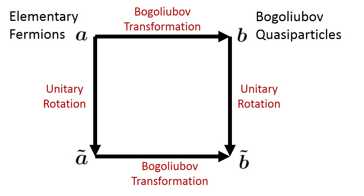
Fig. S1 illustrates the series of transformations that we perform in order to express in a transparent form. First, we unitarily rotate the elementary fermions operators into a new basis of fermionic operators (where the ’s are linear combinations of only ’s but not ’s). While the states destroyed by operators carry well defined spin and angular momentum quantum numbers, and respectively, they are not energy eigenstates of the non-interacting Hamiltonian. In a similar spirit, we will unitarily rotate the quasi-particle operators into a new basis of quasi-particle operators . Importantly, since this operation does not mix quasi-particle creation and annihilation operators, the ground state is still defined as the vacuum with respect to positive energy excitations and hence satisfies and .
Having established these new bases, we will then relate the rotated fermions to the rotated quasi-particles through a Bogoliubov transformation akin to Eq. (S12). This relation then allows us to express in terms of the rotated fermions in a manner that makes explicit the nature of pairing in the ground state since it naturally distinguishes between paired and unpaired states. We note that the purpose of these transformations is not to diagonalize the BdG Hamiltonian (which is diagonalized by the original Bogoliubov transformation Eq. (S12)) but rather to explicitly construct the ground state wave function for an -wave SF with an MQV.
We now discuss the above procedure in detail. To begin, we first invert Eq. (S12) and write the unitary Bogoliubov transformation as
| (S16) |
where are and are dimensional matrices, respectively. Next, we perform a singular value decomposition on the matrices and , where are unitary matrices and is a rectangular diagonal matrix with non-negative real entries. We then perform unitary rotations on the elementary fermions and the Bogoliubov quasi-particles, and ,
| (S17) |
It is straightforward to check that these transformed operators satisfy the canonical anti-commutation relations. In this new basis, the Bogoliubov transformation is expressed as
| (S18) |
where and . Before proceeding with the construction of the ground state, it is necessary to establish some properties of and . In particular, we will show now that in the presence of a non-trivial spectral asymmetry , either one of or have entries on the diagonal which are equal to one. To prove this, let us assume without loss of generality that . Since the Bogoliubov transformation is unitary, the transformation matrix satisfies . This leads to the conditions
| (S19) |
Since and are Hermitian matrices, they have real eigenvalues and eigenvectors,
| (S20) |
Eq. (S19) then implies
| (S21) |
The singular values of , however, are the square roots of the non-zero eigenvalues of both and . Since has exactly more eigenvalues than , those extra eigenvalues must necessarily be zero. This in turn implies that has unity eigenvalues, or equivalently, that has precisely unity entries on the diagonal. In addition, since is a rectangular diagonal matrix, its last rows contain only zeros.
Following this discussion, in general for any and we can define the quantities and . Using the fact that , we can also show that and . From this, it follows that
| (S22) |
Combining the above results with the unitarity of the Bogoliubov transformation Eq. (S18), we conclude that in the presence of spectral asymmetry we will have cases where or , which will give rise to unpaired fermions in the ground state.
Specifically, we find that the Bogoliubov transformation Eq. (S18) splits into three classes
| (S23) |
| (S24) |
and
| (S25) |
where we have omitted the superscript to simplify notation. Physically, these three classes correspond to three different kinds of quasi-particle operators [41]:
- •
Occupied levels Eq. (S23) are those where or . These operators create a unitarily rotated fermion with unit probability.
- •
Paired levels Eq. (S24) are those for which and are non-trivial superpositions of and .
- •
Empty levels Eq. (S25) and are linear superpositions of ’s and ’s, respectively. These operators annihilate the Fock vacuum .
The ground state is still the vacuum with respect to all positive energy quasi-particles and, in terms of the unitarily rotated Bogoliubov quasi-particles, it is given by with
| (S26) |
where the restricted product runs over all paired and occupied levels. Since empty levels annihilate the Fock vacuum, they are not included in Eq. (S26). By construction this state satisfies
| (S27) |
for all and . We can further simplify the ground state since it factorizes into unpaired and paired terms,
| (S28) |
The first two terms in the product clearly indicate that for , there are unpaired fermions in the ground state. Following [40], we can now write the paired part of the ground state in terms of creation operators of elementary (unitarily rotated) fermions
| (S29) |
where the kernel satisfies
| (S30) |
with .
In order to derive Eq. (6) in the main text, we note that we can express the conserved operator in terms of the elementary fermions as
| (S31) |
where the last equality follows since the ’s are unitarily related to the ’s. Since the set of operators that appear in the exponential part of anti-commute with those that appear in the products (unpaired fermions), we can consider the action of on these separately. First, we evaluate the commutator
| (S32) |
and similarly,
| (S33) |
which follows from the usual anti-commutation relations satisfied by the rotated fermions . Next, we consider the action of on the exponential (paired) sector of the wave function. This is done by first calculating the contribution from the spin sector,
| (S34) |
and then observing that the contribution from the spin sector
| (S35) |
exactly compensates for that coming from the spin sector. Hence, we see that commutes with the exponential part of the wave function and so the paired levels do not contribute to ,
| (S36) |
Since the ’s are unitarily related to the ’s, is also the Fock vacuum with respect to . Putting the above together, we hence find that the eigenvalue of the operator when evaluated in the ground state , with given by Eq. (S29), is
| (S37) |
where .
I.3 C. Analytic solution for vortex core states
We generalize the CdGM method [13] for obtaining the vortex core bound states in an -wave superconductor to the case of multiply quantized vortices. For a step-like pair-potential, an explicit solution was obtained previously in [59, 60]. The procedure presented here applies more generally to any pairing term and agrees with that calculation where the regimes of validity overlap.
We start with an -wave state with a vortex of vorticity . The (symmetric) gap function is thus where and . The BdG equations are hence
| (S38) |
Separating the angular and radial dependence of the BdG solutions, we let
| (S39) |
where if , such that Eq. (S38) becomes
| (S40) |
We now rewrite these equations in the form
| (S41) |
where we have defined and .
In order to derive an analytic solution for these coupled equations, we introduce a radius such that , where is the Fermi momentum and is the coherence length. We then consider the BdG equations (S38) separately in the limits where and where . Demanding that the wave function be continuous, we then match the solutions from these two regimes at to arrive at a solution that holds over the entire range.
We first consider the limit where . For physically relevant pairing terms, in this limit and we are hence justified in ignoring the pairing term. The BdG equations (S38) thus decouple in this limit,
| (S42) |
The solutions to these equations are Bessel functions parametrized by . Since we are interested in understanding the nature of the vortex core states close to zero energy, we make an additional approximation and consider energies such that . Reinstating all the proper units, this corresponds to
| (S43) |
where we have defined . Thus, the solutions for are
| (S44) |
where and are arbitrary constants and where the Bessel functions of the second kind are chosen to have vanishing amplitudes since we require a well behaved solution in the limit .
Next, we consider the case where . In this limit, we expect that the pairing term is approximately constant . Hence, we write the BdG solutions as rapidly oscillating Hankel functions enveloped by functions that vary slowly i.e.,
| (S45) |
where are Hankel functions of the first and second kind. Substituting this ansatz into the BdG equations (S38) and considering only the component of the solution (since the other follows from this immediately), we find
| (S46) |
Here, . Since we are in the regime , we use the asymptotic expansion for the Hankel functions
| (S47) |
and drop the terms , which is justified since we are considering the limit . With these further approximations, we find that the slowly varying envelope functions satisfy
| (S48) |
To solve these coupled equations, we treat the right hand side as a perturbation. To zeroth order,
| (S49) |
Imposing the condition that the solutions remain well behaved as , we find that the solutions are
| (S50) |
In order to find the solution to first order in , we make the ansatz
| (S51) |
which when substituted into Eq. (S48) leads to
| (S52) |
Approximating , this is equivalent to
| (S53) |
the solution to which is
| (S54) |
With this, we find that the leading order solution of Eq. (S38) in the limit is
| (S55) |
with given by Eq. (S54).
We have thus constructed the general solution of the BdG equations (S38), with the solution in the limits and given by Eq. (S44) and Eq. (S55) respectively. In order to completely fix the undetermined coefficients and to get the quantization condition on the energy, we demand that the solution be continuous and match the solution in the regime with that in the regime .
Since we wish to extend the solution for Eq. (S44) to the vicinity of , we use the asymptotic expansion
| (S56) |
such that Eq. (S44) becomes
| (S57) |
Similarly, we want to extend the solution from the opposite regime () towards the vicinity of and we use the asymptotic expansion
| (S58) |
such that Eq. (S55) becomes
| (S59) |
where . We must now match the solutions from Eqs. (S57) and (S59) at in order to find a continuous solution.
We first match . Making the ansatz and and matching the solutions at leads to a condition on
| (S60) |
Next, we match , which leads to
| (S61) |
Here, . Comparing Eqs. (S60) and (S61), we find that the parameter is
| (S62) |
Thus, we find that at the function is approximately
| (S63) |
However, recall that we earlier found that is given by Eq. (S54) while constructing the BdG solution in the regime . Hence, in order to have a consistent solution, we must compare the approximate solution Eq. (S63) with Eq. (S54). Since we want to understand the behavior of in the regime where , as a first approximation we can drop the term . This is justified since the pairing term approaches 0 at least linearly and, as we are working in the regime where , we can approximate this term as . Thus, in order to understand the behavior of in the vicinity of we need only consider the integral
| (S64) |
We write where
| (S65) |
We can now approximate as
| (S66) |
and can further write
| (S67) |
Integrating by parts, we find
| (S68) |
We can then approximate as
| (S69) |
since we only make an exponentially small error in extending the integral (which is further suppressed by a factor of ) over the entire range. Thus, we approximate Eq. (S64) as
| (S70) |
In the vicinity of , we hence find that the function (Eq. (S54)) is approximately
| (S71) |
Comparing this asymptotic behavior with Eq. (S63), we find the vortex core energies
| (S72) |
where
| (S73) |
For an elementary vortex , is a half integer, and thus with , we reproduce the CdGM solution [13]. For an MQV with , we see that we cannot get a zero-energy solution since . Moreover, for any , we find branches of vortex core states by taking the appropriate values of such that since our calculation is only valid in this regime. While our method does not reproduce the detailed structure of the sub-gap states away from zero energy, it allows us to analytically estimate the spectral asymmetry, since we can extract the separation between the branches from the spectrum found above.
In order to better understand the nature of the vortex core states, we now consider the specific pairing profile used in our numerical analysis,
| (S74) |
Since the coherence length , we find that
| (S75) |
where and . From this, we then see that the mini-gap and furthermore, we find (pseudo) zero-energy states when
| (S76) |
where . Imposing the condition , we see that we should restrict to which gives us exactly branches of vortex core states. Our calculation thus demonstrates that the angular momenta where the branches cross zero energy, called crossing points in the main text, are separated by an amount , in agreement with our numerical results. Furthermore, we observe that taking a different form of the pair profile simply changes the constant (e.g., for , we find ) but does not affect the scaling of the crossing points with and .
We note that while the spectrum for chiral states with singly quantized vortices has previously been calculated [61], the method presented here easily generalizes to chiral states with MQVs.
I.4 D. Observables from BdG solutions
The particle number and OAM in the BCS ground state can be found by numerically diagonalizing the BdG Hamiltonian . To obtain a finite spectrum we introduce a cutoff on the radial quantum numbers such that is a Hermitian matrix. The eigenstates of the BdG Hamiltonian satisfy
| (S77) |
and are normalized as . Given these, we obtain
| (S78) |
where the sum over is restricted to the positive part of the energy spectrum.