A “Quantal Regret” Method for Structural Econometrics in Repeated Games
Abstract
We suggest a general method for inferring players’ values from their actions in repeated games. The method extends and improves upon the recent suggestion of (Nekipelov et al., EC 2015) and is based on the assumption that players are more likely to exhibit sequences of actions that have lower regret.
We evaluate this “quantal regret” method on two different datasets from experiments of repeated games with controlled player values: those of (Selten and Chmura, AER 2008) on a variety of two-player 2x2 games and our own experiment on ad-auctions (Noti et al., WWW 2014). We find that the quantal-regret method is consistently and significantly more precise than either “classic” econometric methods that are based on Nash equilibria, or the “min-regret” method of (Nekipelov et al., EC 2015).
1 Introduction
Motivation
Consider some on-line computational platform where users interact repeatedly in some strategic context. Natural examples abound including ad-auctions, dating sites, or dynamic allocation of cloud resources. In such settings human players are interacting in some repeated strategic game that is defined by the platform. The on-line platform observes the players’ actions in this game (e.g., a sequence of bids in an auction), but does not have access to their private information (e.g., players’ values in the auction). This latter information is what is really important to the designer and to the users of the platform, as the goals and the level of success of the platform are really defined in terms of this “real world” underlying information. Thus, reliable estimates of this private information are essential for the platform designer to evaluate how well does his platform do, or how may it further be improved. For example, the identification of cases where the revenue (or welfare) of an on-line auction platform may be improved requires reliable estimates of the players’ true values in these cases. Can we reliably estimate the unknown private information of participants from their observed actions?
This challenge has received specific attention in the case of ad-auctions: [Varian, 2007, Athey and Nekipelov, 2010] invoke “classic” econometric methods assuming that players are close to an equilibrium, and as the equilibrium is a function of the private values of the players, they compute in the inverse direction and deduce the private values from the observed equilibrium. This econometric assumption that players reach equilibrium is rather problematic: first, it is often quite unclear which equilibrium to assume: Pure Nash? mixed-Nash? Which one of the multiple ones? Correlated? Bayes-Nash? Which prior? Even more importantly, do we really expect humans to reach a mathematically-defined equilibrium? A much more robust approach was suggested in [Nekipelov et al., 2015]: they instead assume that players are able to (almost) minimize their regret. Formally, this is a weaker assumption since whenever players reach an equilibrium (any Nash, correlated, or even coarse-correlated one) they also minimize their regret. Furthermore, this assumption seems more plausible from a human behavior perspective. In a previous paper [Nisan and Noti, 2017], we evaluated this “min-regret” econometric method on data from an ad-auction experiment that we have previously performed [Noti et al., 2014], and found that it was indeed at least as good as the previous “equilibrium-based” methods. Unfortunately there was only a minor – usually not statistically significant – improvement in the rather low estimation precision.
In this paper we propose a new method for this estimation, one that does not assume that players exactly minimize their regret but rather only that they are more likely to behave in less regretful ways. This is similar in spirit to “quantal response” modeling of human behavior in games [McKelvey and Palfrey, 1995], but is applied to the regret in the repeated game rather than to utilities in a single game. The method is general and easy to implement, and should apply to most computerized repeated game settings. We evaluate our method – and compare it to previous methods – not only on data from our ad-auction experiment, but also on data from an experiment of [Selten and Chmura, 2008] on repeated two-player 2x2 games (a context in which we are not aware of any previous work on this estimation task.)
Let us start by demonstrating our method (and previous ones) on a simple example.
An Example
Consider the following 2x2 two-player game in figure 1(a), where we are only given six of the eight parameters defining the game, and need to infer the unknown ones, and , from empirical data on players’ actions when repeatedly playing the game. This game (with some specific values of and ) is one of those that [Selten and Chmura, 2008] have run in experiments with human subjects, and the empirical frequency of play in one of their sessions is given in figure 1(b). What would your prediction of the missing parameter be?


A classic equilibrium-based approach would be to assume that the players reach (approximately) a mixed Nash equilibrium of the game. In the single mixed equilibrium of the game, the column player must be playing with a probability , so we can estimate .11 1 Note that since we must have , and indeed otherwise is dominated by .
An adaptation of the regret based approach suggested by [Nekipelov et al., 2015] would assume that players (nearly) minimize their regret. Under this assumption it would calculate for every possible value of , what would have been the regret of the row player, had the missing parameter been . The regret here is defined as the difference between the utility that could have been obtained using the best fixed strategy in hindsight (and the other players still behaving as they did empirically) and the utility that was obtained under the empirical play. For example, for the row player’s empirical utility is , while had he always played his utility would have been and had he always played his utility would have been . Thus the row player’s regret is . More generally, one may calculate the regret of the row player for every possible value of (in some grid in some valuation range), by: . The regret of the row player as a function of the “hidden value” is graphed in Figure 1(c). The basic “min-regret” method would take as its estimate the value with the lowest regret,22 2 The specific implementation in [Nekipelov et al., 2015] actually looked for the lowest relative regret, but as we demonstrate in Appendix A, using absolute regret gives better estimates, so in the rest of the paper we use the simpler and more precise absolute regret method as a tougher benchmark for comparison. which happens to be .33 3 Here we are assuming that possible values are only integers; it is not difficult to see that the lowest regret among all possible real-valued is obtained at the same point of the equilibrium estimate above, 13.7, as is the case in all 2x2 games (but not generally). As can be seen in Table 1(a), the restriction to integer values gives more precise estimates for 2x2 games, so, again, we use the more precise method as a tougher benchmark for comparison.
Our suggested quantal regret method would first take into account that humans are never exact optimizers. It would then look at the regret graph (1(c)) and notice that it is much steeper to the right of the min-regret point than it is to its left. Thus, it may seem more likely that the real value of is lower than 13 (where the player only loses a bit from acting the way he did) than that it is higher than 13 (where the player loses a lot). We may utilize this observation by taking a weighted average of the possible values of , where the weights are decreasing with the regret. Specifically, we take exponentially decreasing weights, as follows: . For a value of (say) this would evaluate44 4 The summation in this example is over integers in the range , although due to the exponential decay, values over 20 or so have essentially no effect on the result. to . As the value of the “regret aversion” constant grows to infinity, the quantal regret estimate approaches the min-regret estimate.
For the curious reader let us reveal that in the actual experiment of [Selten and Chmura, 2008] the value taken was , and indeed in this specific instance the estimate of the quantal regret method was significantly closer to reality than that of the min-regret method of [Nekipelov et al., 2015] which in turn was slightly better than the “classic” method. As we will show below, this is the usual state of affairs in our data: the quantal regret method consistently and significantly outperforms the min-regret method which in turn somewhat outperforms classic methods in the two scenarios of repeated games that we have looked at.
Experimental Results
We have evaluated the qunatal-regret method by computing its error on data obtained in two different experiments of repeated games. In both cases, a game was designed by an experimenter who controlled all of its parameters, and observed humans playing the game repeatedly. We “hid from ourselves” a basic parameter of the game , and tried to infer this hidden parameter using the observed data. We then “un-hid” the actual value of this estimated parameter and compared this real value with our estimate.
We compared three basic econometric methods: a classical one that assumes that players are in an equilibrium (EQ), the min-regret (MR) method suggested in [Nekipelov et al., 2015] and our proposed quantal regret (QR) method. Our basic comparison metric is the root mean square error (RMSE) over the estimation errors in a specific setting. Specifically, the estimation error of an estimate for a parameter whose true value is is the estimate’s distance from this true value, i.e., , and the RMSE of a set of estimates is . We also look at the average of all estimation errors, as well as at the “ hit-rate”, which is the fraction of estimates that are within an interval of from the true value.
| 2x2 Games – Over All Sessions | |||
|---|---|---|---|
| EQ | MR | QR | |
| RMSE | 3.41 | 3.25 | 2.29 |
| Average Error | 2.99 | 2.84 | 2.04 |
| Hit Rate | 68.87% | 75.00% | 81.60% |
| Ad auctions – VCG Sessions | Ad auctions – GSP Sessions | ||||||
|---|---|---|---|---|---|---|---|
| EQ | MR | QR | EQ1 | EQ2 | MR | QR | |
| RMSE | 6.46 | 6.26 | 4.22 | 9.73 | 9.87 | 8.02 | 5.09 |
| Average Error | 5.38 | 5.13 | 3.42 | 7.74 | 8.02 | 6.32 | 3.85 |
| Hit Rate | 61.67% | 63.33% | 81.67% | 48.33% | 41.67% | 56.67% | 81.67% |
Our first dataset is from [Selten and Chmura, 2008], where human subjects were given a two-player 2x2 game and played it for 200 turns.55 5 The exact setup is a bit more complicated as the players were split into “groups” with 4 row players and 4 column players who were re-matched at random with each other for each of the 200 periods. See the details in Section 3. The data that we have is the empirical frequency of play of each of the four possible strategy profiles, , , , , during these 200 plays of the game – exactly like in the example above. 12 different games were investigated, half of which are constant-sum, where for each game we have data from multiple independent sessions: 12 sessions for each of the constant-sum games and 6 sessions for each of the non-constant sum games; for a total of 108 sessions.
For each of these 108 sessions we estimated (separately) each of the 8 parameters (payoffs) defining the game, using each of the three methods. The bottom line, as shown in Table 1(a), is that the quantal regret method has a large and statistically significant advantage over the other two methods, while the min-regret method is just slightly better than the Nash equilibrium method.66 6 As mentioned previously, for this case of 2x2 games, the variant of the min-regret estimator that allows real values would be identical to the Nash equilibrium method. The min-regret method reported here allows only integer values and gives slightly better results since it usually manages to round in the “correct direction” where the regret rises less steeply.
Moreover, these results were very robust: First, the quntal-regret method outperformed the two other methods for each one of the 12 games studied (except for a single one where all three methods gave nearly identical excellent results). Second, we tried several variants of handling the nuanced details of the experiment, and all gave similar results. Third, the method was robust to varying the range of valuations or the grid size that were used for the regret calculation. Finally, the method is robust to the choice of the regret aversion parameter , and Figure 2(a) shows that the quantal regret outperforms the other two methods for a very wide range of values. See Section 3 for more details regarding the setup and the analysis of the 2x2 game dataset.
Our second dataset is from an ad-auction experiment that we ran [Noti et al., 2014]. Each session in this experiment had 5 “advertisers” repeatedly competing for 5 ad-slots, with differing “click through rates” in a sequence of 1500 auctions. This experiment used both the common “GSP” auction rule and the theoretically appealing “VCG” auction rule, and also varied whether players were explicitly given their values or had to “learn” them from their feedback. For each setting there were 6 different sessions (all together 24 sessions with a total of 120 bidders). Each of the five bidders in a session was given a value per click from a fixed set of values. The econometric task tries to recover the value of each of the players only from the sequence of bids of all players in the repeated auction. As mentioned above, in a previous paper [Nisan and Noti, 2017] we compared classical equilibrium-based methods to the min-regret method suggested by [Nekipelov et al., 2015], and the bottom line is that there was a slight – usually not statistically significant – advantage to the min-regret method. Here we find, as summarized in Table 1(b), that the qunatal regret method has a large and statistically significant advantage over both.
Again, the advantage of the quantal regret method is very robust: it holds for each of the different experimental settings (GSP vs. VCG and “Given-Value” vs. “Deduced-Value”) separately, as well as in almost all of the comparisons according to player types. It is also robust to variants of implementation used in the previous paper, such as discarding an initial learning phase or looking at relative error rather than absolute one. Finally, as demonstrated in Figures 2(b) and 2(c), the results hold for a wide range of values of the regret aversion parameter . We provide a more detailed description of the setting as well as describe our analysis in Section 4.


The rest of the paper describes and discusses the qunatal regret method in detail in Section 2, and then goes into the specific analysis of our two datasets in Sections 3 and 4. We believe that the quantal regret method is applicable and can give estimates that are much more precise than existing methods in a variety of repeated game settings. The validation or refutation of this on further datasets is the main challenge that we leave.
2 The Quantal Regret Method
2.1 Setting
We are looking at players repeatedly playing a game. We have partial information about the game, where the unknown information is captured by a parameter , and the game is defined by known utility functions . We are given the actual play of the players for a duration of repetitions of the game: at each time step , each player has played the action , where is player ’s action space. Our task is to estimate the unknown parameter given the observed behavior of the players. We also have some prior on the possible values of .
In the most common special case we have that (1) , where captures all unknown information about the “value” of player , i.e., that the utility functions are given by ; (2) the ’s are independent of each other, i.e., ; and (3) the distribution is simply uniform over (and thus also the marginal distributions are uniform).
2.2 The Method
The quantal regret method takes the actual play as input and computes (in principle) for each possible and for each player , the player’s regret had his utility in the game been defined by this value of :
Our prediction from player is given by the weighted average of the possible values of , where the weight of each is updated from the prior in a way that is exponentially decreasing with its total regret. I.e.:
| (1) |
where the normalization constant is given by .
In the common special case defined above, the regret of each player only depends on , which implies that each can be evaluated separately: , where the normalization constant is given by . In natural cases where the are scalar (or low-dimensional) it is feasible to literally compute for every possible value of (at least in a sufficiently fine grid), and then explicitly compute the weighted expected value with these weights.
We note that this method is general and quite easy to implement: calculating the regret of a given player for a given possible value of and an empirical sequence of play is straightforward from the definition, as long as the set of possible actions of the player in the stage game is small enough. For a continuous range of actions, taking a fine enough grid will certainly suffice. The method requires also going over all possible values of . In the common case where and each captures the information for a single player , as mentioned above, each of these can be computed separately, and each of these is typically low-dimensional enough as to feasibly allow trying all values in a reasonably fine grid.
This method is parametrized by the regret aversion parameter . A value of close to zero corresponds to the regret having no significant effect on players’ behavior, in which case we get very little information from the empirical play and our estimate is simply the expected value of according to the prior distribution. A very large value of implies that players are much more likely to act in a way that has less regret than one with more regret, and thus the prediction becomes the maximum likelihood , which is the basic form of the suggestion in [Nekipelov et al., 2015]. A reasonable choice for the value for would depend on our assesment of the minimal gap in utilities that our human players would consider significant in the specific type of game that is considered. A reasonable rule of thumb for games with non-negative “values” could take to be a few percentage points of a player’s typical value in the game. Choosing to be the inverse of would mean that we assume that a regret that is larger by amount is times less likely. For high-stakes games, or games that are well understood by the players, or if the prior knowledge of the range is especially poor, could reasonably be somewhat increased. In this paper we use “round” values of that correspond to being about of the “average value” in the game. We also discuss the empirically optimal values of and demonstrate that rather wide ranges of values of still give good estimates.
2.3 The Procedure
Next we describe how to apply the quantal regret estimation method. For concreteness, we exemplify all the technical details in a simple first-price auction setting, and the generalization to any other game setting is straightforward. In our first-price auction, each player has a private value for the auctioned item, which we do not know and seek to estimate. We may assume that we do know some bounded range from which these may come, and due to any lack of further knowledge we assume a uniform prior over this range. We observe a sequence of bids of the players for repetitions of this auction (each time for a fresh copy of the good, where players’ values remain constant throughout).
An equilibrium-based approach would perhaps assume that players somehow approach a Nash equilibrium of the full information game (since the repetitions presumably allowed them to learn the information required for that), which has the highest-value player bidding just above the second-highest value, and the second-highest player bidding his true value. The actual value of the highest bidder and the values of other bidders do not affect this equilibrium and in principle could not be estimated using the equilibrium assumption.
Here, in contrast, is an implementation of the quantal regret method:
- 1.
First we choose a reasonable grid on of possible values. Since it is hard to believe that our estimate will have less than a error (of the interval size), it seems that taking the grid points is good enough. Let us denote the points on the grid by .
- 2.
For notational convenience, let us denote by the set of time steps in which won the auction, i.e., .77 7 Throughout this example we assume that wins ties; more generally, one should adjust the expressions according to the tie breaking rules.
- 3.
Next, for each player and each possible grid value , we calculate the regret of player had his value been :
- (a)
The player’s empirical utility had his value been is .
- (b)
To calculate the optimal fixed bid for player , had his value been , let be the number of times that bidding would make player the winner of the auction. So . Algorithmically, one may perform this maximization by exhaustive search over the possible . In principle, one has to go over all maximal bids of other players, but often there will be some bidding grid that is implied by the auction setting, or one may alternatively use our grid for the bids.
- (c)
Now the regret is:
- (a)
- 4.
We now need to choose a value for . One may roughly follow the rule of thumb suggested above and take , where is, say, of the average bid.
- 5.
Our total estimate for each would be .
2.4 Rationale
The basic assumption behind this method is that players tend to succeed in minimizing their regret in a long repeated play, however they do not do so perfectly but rather are less likely to achieve higher regret than to achieve lower regret. This assumption – which this paper tests empirically – makes sense from several perspectives.
As argued in [Nekipelov et al., 2015], the basic ability
of players to learn enough about the environment as to be able to minimize their regret is a rather weak assumption,
and in particular is strictly weaker
than assuming that they reach a Nash equilibrium or even a correlated [Aumann, 1974] or coarse-correlated [Young, 2004] one (since in
any such equilibrium the players must all be minimizing their regret). Furthermore, there are many natural dynamics
that are known to indeed minimize regret in the long run – see, e.g., [Blum and Mansour, 2007, Arora et al., 2012, Hart and Mas-Colell, 2000].
Note also that such dynamics
are possible even when players have very little knowledge about the game that they are playing, but only
receive feedback about their utilities (the “bandit” setting).
Nevertheless, it is worth emphasizing that this assumption is far from trivial in two senses: first that the players
are sufficiently smart and rational and posses sufficient information as to succeed in minimizing their regret, and,
second, that the players are not even smarter and cooperative as to reach a threat-based equilibrium of the repeated game
which may have high regret even though it may Pareto-dominate all equilibria of the stage game.
It is possible to justify the quantal regret method as the one that minimizes the expected square error after a Bayesian update of the prior based on the assumption that the regret affects the probability that a player plays any particular sequence of actions in a way that is proportional to . Formally our assumption is that where is some prior likelihood of the sequence and is just a normalization constant ensuring that all probabilities sum to : . While in this formula may depend on , we further assume, simply due to lack of any knowledge, that it is a constant.88 8 This assumption cannot really be interpreted as a direct reasonable model of the world, but since our assumption regarding is really quite under-specified (i.e. it could be that each has a separate set of possible in it support), together these assumptions suggest our lack of knowledge about beyond that given by the prior.
Once we take this behavioral assumption then our estimate is simply the one that minimizes the posterior expected square distance between and . Specifically, using Bayes’ rule on our assumption that yields that the posterior probability over after observing the sequence of actions to be: . The estimate that minimizes the expected square error, is exactly the weighted average according to this posterior, which is how we chose our estimate.
3 Estimation in 2x2 Games
3.1 The 2x2 Game Dataset
The first dataset that we use to evaluate the quantal regret method is from an experiment of repeated 2x2 games of [Selten and Chmura, 2008]. In their experiment they investigated 12 games for two players (“row” and “column” players), 6 of which were constant sum and 6 non-constant sum games. Each of the games had non-negative utilities and was “completely mixed”, i.e., had only one equilibrium point in which every pure strategy is used with positive probability. The utility matrices of the games are fully depicted in Appendix B. There were 12 independent subject groups (‘‘sessions’’) for each constant sum game and 6 for each non-constant sum game, to a total of 108 sessions. Each session consisted of eight human players -- four in the role of the row players and four in the role of the column players.99 9 In fact, [Selten and Chmura, 2008] ran two independent subject groups of eight players each in every session, however here we refer to each independent subject group as a separate session. For the full details regarding the experimental setup see [Selten and Chmura, 2008].
In the beginning of every session, the players were informed about the game matrix, including the payoffs of both players. They interacted over 200 periods, always in the same role, and were re-matched in every period within their subject group. In each period every row player had to choose between two actions and , and every column player chose between and . After each period, every player received feedback about the other player’s choice and payoff, period number, and their cumulative payoff. In the end of the experimental session, every player was paid proportionally to his accumulated payoff in addition to a show up fee.
The data consist of the utility matrices of the 12 games, as well as of the empirical frequency of play for each player over his 200 plays. Specifically, for each of the 8 players, in each of the 108 sessions, we observe the empirical frequency of each of the 4 strategy profiles: , , , , during the 200 periods. For illustration, Figure 1(a) presents one of the games in the dataset (with one pair of utilities hidden for estimation), and Figure 1(b) shows the average of the empirical frequency of play that was obtained in one of the sessions of this game.
3.2 The Quantal Regret Method in the 2x2 Game Setting
Our econometric estimation task in the 2x2 game setting is to estimate each of the 8 parameters defining the game (the 4 utilities of the row player and the 4 of the column player), using the observed data. Specifically, we “hid from ourselves” each of the 8 parameters, one at a time, and attempt to infer this hidden parameter using the empirical frequency of play and the rest of the (unhidden) parameters.
In this section we define the estimation in the session level, which is the general level that ignores the specific experimental setup described above, and in the next section we show the robustness of the results to other levels of estimation. In the session-level approach, we compute for each independent subject group (session) the empirical play by averaging the empirical frequencies of the eight players in the group (for each of the four strategy profiles). We consider this average as if it was the empirical frequency played by two (global) players in the session, and use it to estimate the 8 parameters in the game – 4 parameters of the (global) row player and 4 of the (global) column player.
We applied the quantal regret method according to the procedure described in Section 2.3, to estimate the 8 parameters in each session. In this section we set the regret aversion parameter by , which corresponds to of about 3% of the average value in the games (as suggested in Section 2.2), and for each session, the regret for each of the two players was computed for each of his 4 parameters over the integers in the interval . In the next section we show the robustness of the results to different implementation variants.
We compare the estimates obtained using the quantal regret (QR) method with those obtained using the min-regret (MR) and the equilibrium-based (EQ) methods. As described in Section 1, the min-regret method takes as the estimate the value that minimizes the regret. The equilibrium-based method assumes that the empirical frequency of play is the mixed Nash equilibrium of the game, and utilizes it to derive value estimate for each of the parameters, as was demonstrated in Section 1. For a fair comparison, since the estimates of the regret-based methods are restricted to the parameter range , we keep the EQ estimates in the same range. We define the session estimation error as the RMSE over the estimation errors of the 8 parameters in the session, and, as explained in Section 1, we compare the success of the estimation methods based on the RMSE, on the average of the estimation errors, and on the hit-rate, in a given setting.
Table 1(a) presents the bottom line of the comparison results over all 108 sessions in the experiment. It clearly shows that the quantal regret method outperforms the two other methods, which in turn have similar performance with a small advantage to the min-regret method (as could be expected, since the MR method rounds the EQ estimates in the correct direction, see Section 1). Specifically, the RMSE of the QR method was far lower than the RMSE of the MR and the EQ methods, and the difference was statistically significant: the estimation errors using the QR method were significantly lower than the errors using each of the other two methods (paired two-sided Wilcoxon signed rank test, N=108 sessions, ). In addition, although smaller, the difference between the errors of the MR and the EQ methods was statistically significant (). Moreover, Table 1(a) shows that the quantal regret method has the highest hit-rate, with 81.6% of the parameter estimates within a delta of 3 from the true values.
The quantal regret method outperforms the other two methods also when considering the constant and the non-constant sum games separately. Table 2 shows the estimation results over the 72 sessions of the constant sum games and over the 36 sessions of the non-constant sum games. It can be seen that for both types of games, the RMSE of the QR method is lower than the RMSE of the other methods, and the differences were statistically significant at the 1% level in both cases (paired two-sided Wilcoxon signed rank tests, N=72 or 36 sessions). Also the errors using the MR method were significantly lower than those using the EQ method at the 1% level for both types of games. Moreover, Table 9 shows that the quantal regret outperforms the other methods in each of the 12 games separately; except for Game 6 for which all methods perform very well, the QR method has lower RMSE than the others in estimating each of the games, and usually by a large gap.
| Constant Sum Games | Non-Constant Sum Games | |||||
|---|---|---|---|---|---|---|
| EQ | MR | QR | EQ | MR | QR | |
| RMSE | 3.42 | 3.27 | 2.14 | 3.39 | 3.23 | 2.57 |
| Avg Err | 3.02 | 2.86 | 1.93 | 2.93 | 2.81 | 2.25 |
| Hit Rate | 69.27% | 75.00% | 83.68% | 68.06% | 75.00% | 77.43% |
3.3 Robustness of the Results
After seeing that one implementation of the quantal regret method manages to estimate the 2x2 game dataset better than the other two methods, let us now show that this is robust to other implementation variants.
Robustness to the estimation level
In the previous section we took a general approach and tested the session-level estimates. We tried several variants of handling the specific setup of the experiment, where in every session there were 4 row players and 4 column players, who were re-matched in every period, and thus interacted directly or indirectly with each other (see Section 3.1). First, we estimated the parameters in each session by a fine grained aggregation of the players, i.e., by aggregating the 4 row players and the 4 column players separately. For the regret-based methods QR and MR, this implies deriving the 4 parameters of players of the same type by their total regret. For the QR method this is exactly like Equation 1 specifies, with reduced proportionally to 3/4. Table 3 shows that although this fine grained aggregation of the players improved the MR results relative to its session-level results, it hardly affected the QR results, and overall the results remained qualitatively the same.
Second, we tried to derive the parameter estimates in the player-level, obtaining 4 estimates from each of the 8 players separately for each session. This approach, that derives the estimates based on less information and is thus more prone to noise, increased the error for all three methods, as could be expected. Third, taking a more general approach and deriving the parameter estimates in the game-level (i.e., based on the average of the empirical frequencies over all sessions for a game), improved the estimation results for all three methods, as expected. Table 3 summarizes the estimation results and shows that overall the results reported in the previous section, where the QR method outperforms the other methods, are robust to the different estimation levels.
| Estimation Level | EQ | MR | QR | |
|---|---|---|---|---|
| Game-level estimate | RMSE | 3.12 | 2.91 | 2.01 |
| Average Error | 2.71 | 2.54 | 1.76 | |
| Hit Rate | 72.92% | 77.08% | 82.29% | |
| Session-level estimate (Baseline) | RMSE | 3.41 | 3.25 | 2.29 |
| Average Error | 2.99 | 2.84 | 2.04 | |
| Hit Rate | 68.87% | 75.00% | 81.60% | |
| Fine grained aggregation of players | RMSE | 3.41 | 3.04 | 2.30 |
| Average Error | 2.99 | 2.63 | 2.05 | |
| Hit Rate | 68.87% | 78.70% | 81.13% | |
| Player-level estimate | RMSE | 4.72 | 3.40 | 2.95 |
| Average Error | 4.57 | 3.08 | 2.77 | |
| Hit Rate | 56.66% | 73.15% | 73.29% |
Lastly, while up to here the estimation was for a general 2x2 game, estimation for the constant sum games can take into account the constant sum property of the game. In this case, the estimation task is of estimating only 4 parameters rather than 8 (e.g., the 4 payoffs of the row player), and these parameters can be estimated from the aggregation of the two players in the session-level. In Appendix F we show that, as expected, the aggregation of the two players improves the estimation results for all the three estimation methods. We note though that the improvement for the MR method is sharper and in the aggregated case it outperforms the QR method.
Robustness to the parameter selection
Let us now return to the session-level estimates and show that the results presented in the previous section are robust to different selection of the parameters. First, while we demonstrated that the quantal regret method outperforms the other methods using the regret aversion parameter , it is in fact true for all reasonable values of . Figure 2(a) shows the RMSE of the quantal regret method as a function of the parameter , for all 108 sessions, compared with the RMSE of the min-regret and the equilibrium-based methods. As can be seen, the RMSE of the quantal regret method is consistently lower than the RMSE of the other methods, and as expected approaches the RMSE of the min-regret method as grows large. The best results with RMSE of 2.29 are achieved at . For very low values of where the quantal regret method effectively doesn’t consider the regret levels in the estimation process, the error is large.
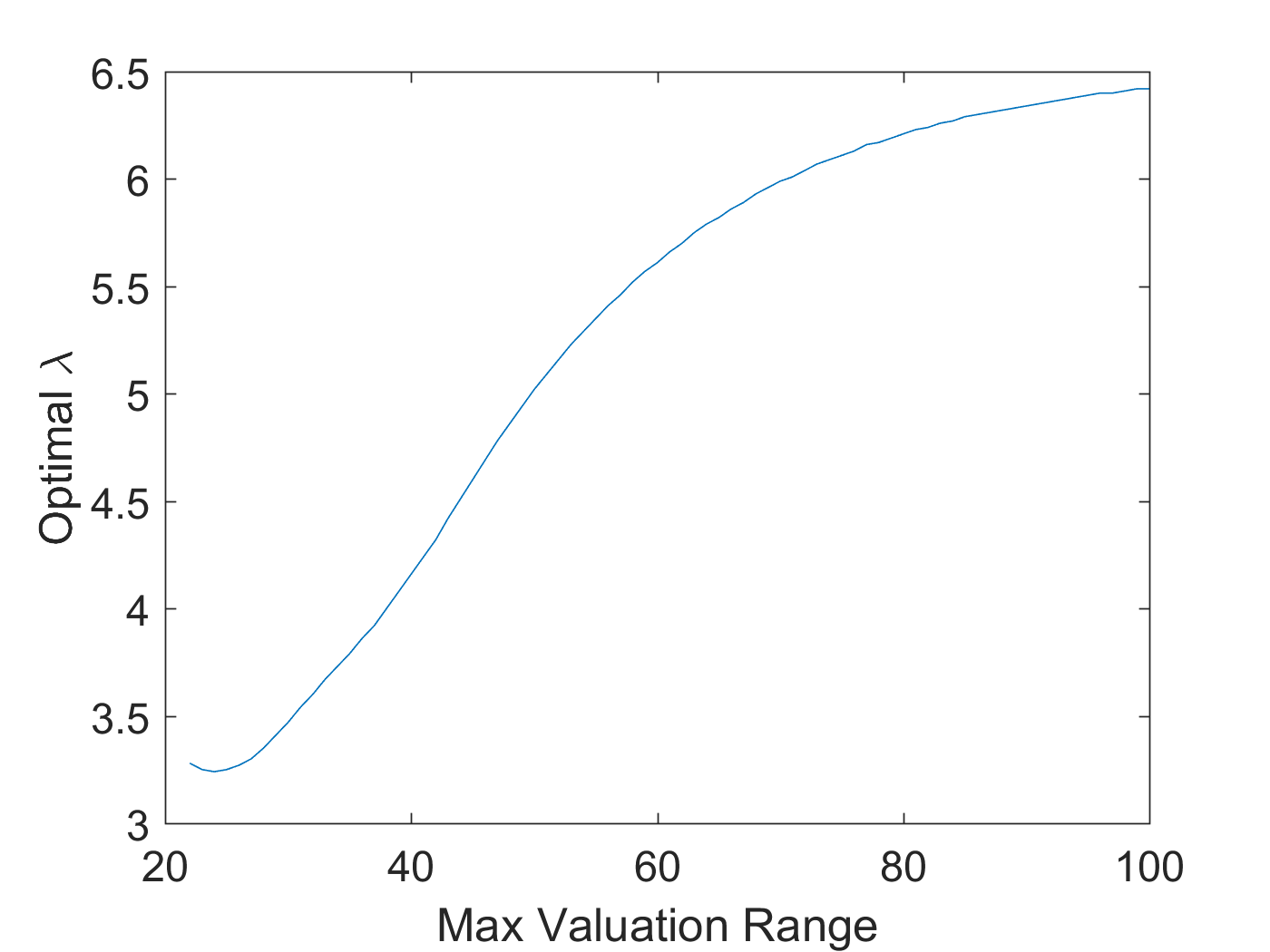
Second, in the previous section we assumed that we know a quite accurate range of valuations from which the parameters may come, however good results are obtained even when the prior is much less accurate, as is shown in Figure 3(a). The graph also shows that with a less accurate prior it is better to use a higher value, while for a good prior it is better to use a lower value, and Figure 3(b) shows how the optimal value of increases with the valuation range that is considered. Finally, Table 7 in Appendix F shows that the quantal regret is robust to varying the resolution of the grid being used for the regret calculation, while as expected with a more accurate grid the min-regret estimates become closer to the equilibrium-based estimates.

4 Estimation in Ad Auctions
4.1 The Ad Auction Dataset
The second dataset is from a previous experiment that we ran, where human subjects were asked to participate in a simulation of ad auctions, similar to those held by search engines like Google or Microsoft (also known as “sponsored-search auctions”). This experiment was described in [Noti et al., 2014], which contains all the details as well as the results. In the experiment, groups of five participants simulated the roles of advertisers and had to compete in a stream of ad auctions that lasted 25 minutes. The auctions were conducted continuously, one auction per second, to a total of 1500 auctions. The participants could modify their bids at any time, and each auction was performed with the current settings of the bids. Each player was assigned a “type” at random, which was his private “valuation,” i.e., the monetary value that he obtained from each user who clicked on his ad (we used 21, 27, 33, 39, 45 “coins”). Players did not know the values of the other players nor the bids that the others made. Each ad auction sold five ad positions with varying (commonly known) Click Through Rates (CTR) (we used 2%, 11%, 20%, 29%, 38%), which were displayed in a decreasing order of CTRs, such that the position on the top of the page received the highest CTR. Every time an advertiser with a valuation won a position with CTR , he got an income of from that auction. This income was added to his balance and the appropriate payment according to the auction rule was deducted from his balance. The players were given a graphical user interface in which they could modify their bids as often as they wished, and follow the results of the auctions so far. Appendix D presents a screen shot of the user interface. In the end of the experiment players were paid for their participation proportionally to their final balance (in addition to a fixed participation fee).
The experiment had a two-way (2x2) between-participant design; thus there were four experimental conditions. The two factors were:
- 1.
Payment Rule (the Auction Mechanism): The (theoretically appealing) VCG payment rule was compared with the (commonly used) GSP payment rule. Both VCG and GSP auctions make the same allocation of positions – by decreasing order of bids – but their payment rule is different. Unlike GSP, the VCG is truthful; i.e., in every VCG auction it is a dominant strategy for every player to bid his true value (see [Edelman et al., 2007, Varian, 2007]).
- 2.
Valuation Knowledge: While the starting point of analyzing behavior in auctions is the “valuation” of the bidder, it is questionable to what extent users are explicitly aware of this valuation. We compared the case where bidders were directly given their valuation (given value, GV), and were explained its significance, and the case where bidders were not directly given the valuation, but rather only see their payoffs – information from which the valuation may be deduced, but could alternatively be directly used to guide the bidding (deduced value, DV).
There were a total of 24 experimental sessions, 6 sessions for each of the 4 experimental conditions (thus there were 12 sessions for each factor). The groups (of five players each) were randomly assigned to the four experimental conditions, giving a total of = 120 participants. For further details regarding the experimental setup see [Noti et al., 2014].
4.2 The Quantal Regret Method in the Ad Auction Setting
Our econometric task in the ad auction setting is to estimate the private values of the bidders from the observational data in the ad auction game. That is, we now assume that we do not know the private values and wish to recover these values from the observed sequence of bids that was played, the observed CTRs, and the utility functions of the players.
We applied the quantal regret method to derive value estimates for each of the players, as described in Section 2.3. We computed the regret in the ad auction game (over the 1500 auctions) for each of the bidders, over the integer values in the range . Figure 4 presents the regret results as a function of these values, averaged over players of the same type and by the four experimental conditions. The min-regret method suggested by [Nekipelov et al., 2015] takes the minimum point for each player as the estimate for his value, which is clearly visible in the graphs. In contrast, the quantal regret method takes a weighted average of the possible values, with weights that are exponentially decreasing with the regret. In this section we use as the regret aversion parameter, which corresponds to of the average utility in the auction game (as suggested by the rule in Section 2.2), and in the next section we show the robustness of the results to different values of this parameter as well as to other implementation variants.
We compare the estimates obtained using the quantal-regret method with those obtained using the min-regret method and using econometric methods that rely on the standard equilibrium assumption. Since in [Nisan and Noti, 2017] we have already compared min-regret with the standard econometric methods on the same ad auction data, here we focus on the performance of the newly suggested quantal-regret method. We evaluate the results separately for GSP and VCG, since the standard methods are different for these two auctions due to their different equilibria predictions, however notice that the two regret-based methods are general and work just the same for both cases. Again, our main measure for the quality of the estimation methods is the RMSE over the estimation errors in a given setting. Specifically, we compute for every player whose true value is , the absolute estimation error by: , where is the value estimate for player . The estimation error on a set of players is the RMSE of the players in : . Additionally, we look at the average estimation error and at the hit-rate achieved in a given setting, as explained in Section 1.

4.2.1 Evaluating Estimations in VCG Auctions
We start by considering the VCG auction which is a simple case for standard econometrics: in VCG bidding truthfully is a dominant strategy, and so it should be a strong prediction that players will all bid their true value in equilibrium. Thus, the classic econometric method is simply taking the average bid that a bidder played in a sequence of auctions as the estimate for his value in these auctions.
Table 1(b) summarizes the bottom line of the estimation results over all 60 VCG bidders, for the quantal regret (QR) method, the min-regret (MR) method, and the standard equilibrium-based (EQ) method of taking the average bid. It clearly shows that the quantal regret method succeeded much better than the other two methods, which, in turn, had similar performance. Specifically, the RMSE of the QR method was about 30% lower than the RMSE of the others, and the difference was statistically significant: the estimation errors using the QR method were significantly lower than the errors using each of the other two methods (paired two-sided Wilcoxon signed rank tests, N=12 sessions, ). In addition, while the QR method achieved the highest hit-rate of 81.7%, the MR and the EQ methods had very poor hit-rates; only 61.7% of the estimates using the EQ method were withing a delta of 6 coins from the true value, despite the fact that this method is based on the particularly strong prediction of the truthful dominant strategy.
Quantal regret consistently outperforms the other two methods also when considering the estimation errors by information settings and by types of players. Figures 5(a) and 5(b) present the RMSE by the different experimental settings and Table 10 (left column) provides the full estimation results by setting. First, Figure 5(a) shows that both when players are given with their values (the GV setting) or when they have to deduce their own value (the DV setting), the quantal regret method has lower RMSE than each of the other two methods, again by a large gap, and this was significant at the 5% level for both settings (paired two-sided Wilcoxon signed rank tests, N=6 sessions). In addition, all three methods succeed somewhat better in estimating values in the given-value setting than in the deduced-value one, as could be expected, however these differences were not statistically significant for neither of the methods.


Second, also when considering each type separately, we found that the RMSE of the quantal regret method is consistently lower than the RMSE of the other methods, and it achieved much higher hit-rates than the others (see Figure 5(b) and Table 10, except for type 33 for which the min-regret is better). In addition, as was found and discussed in depth in [Nisan and Noti, 2017], using the basic min-regret method there is a significant negative correlation between the estimation error and the player type (, ), indicating that it tends to perform better on the higher type players than on the lower types. The quantal-regret method “flattens” the errors (due to a larger improvement on the two lowest types) and reduces this correlation to only (). Finally, Figure 5(c) plots the average estimates of the three methods alongside the true value for each player type. As can be seen, the three methods tend to err to the same direction, overestimating the values of the lower type players and underestimating the values of players of the highest type.
To conclude, in the VCG setting, the estimates obtained by the quantal regret method are consistently and significantly better than the estimates using the other two methods: it improves upon the min-regret method, as well as upon the standard method that relies on the specific and strong prediction of the truthful equilibrium for the VCG.
4.2.2 Evaluating estimations in GSP auctions
For the GSP auction the situation is much more complicated for equilibrium-based econometric methods, since there are no dominant strategies and there exist multiple equilibria. There are two basic approaches in the literature for deducing bidders’ valuations in GSP auctions, and we use them to compare the quantal regret performance. The first method was suggested in [Varian, 2007] and is based on the assumption that the players reach the “VCG-like” equilibrium of the GSP, which is the equilibrium of the full-information one-shot game that gives the VCG-prices (we denote this method by “EQ1”). The second method was suggested by [Athey and Nekipelov, 2010], where bidders participate in a large number of auctions, and receive feedback that can vary from auction to auction, and the basic assumption is that each bidder is best-responding to the distribution that he faces (we denote this method by “EQ2”). For more details regarding these two methods see Appendix E.
Table 1(b) presents the bottom line of the comparison results of the quantal regret method with the min-regret method and the two “classic” equilibrium-based methods, over all 60 GSP bidders. As can be seen, the quantal regret method outperforms the min-regret method, which in turn outperforms the two equilibrium-based methods. The RMSE of the QR method is far lower than the RMSE of the other methods, and the differences are statistically significant: the estimation errors obtained using the QR method are significantly lower than the errors obtained using each of the other three methods (paired two-sided Wilcoxon signed rank tests, N=12 sessions, ), with an average error of a less than half of that obtained using the two classic equilibrium-based methods. The advantage of the min-regret over EQ1 and EQ2 is also statistically significant over all GSP players (). 1010 10 This is different from the results in [Nisan and Noti, 2017], where MR was found to be significantly different only from the EQ1 method. The difference is due to the use of the entire auction game (rather than using only the second half in [Nisan and Noti, 2017]), and the use of the absolute estimation error (rather than using the relative error) which seems to help the MR method that tends to have higher error on the lower value bidders. In Section 4.3 (Tables 4 and 5) we show that the new quantal regret method is completely robust to these variants. Furthermore, quantal regret is the only method that achieves a reasonable hit-rate with 81.67% of the estimates within a delta of 6 coins of the true value, while all other methods perform poorly and only manage to achieve hit-rates below 60%.


As in the case of VCG, the advantage of the quantal regret method is robust to whether considering the estimation errors by information settings or by types of players, as can be seen in Figures 6(a) and 6(b) and in Table 10 (right column). First, in both information settings GV and DV (Figure 6(a)), the estimation errors using the QR method were significantly lower than the errors using each of the three other methods (paired two-sided Wilcoxon signed rank tests, N=6 sessions, ). In addition, the QR method as well as the other methods have higher error in the deduced-value setting than in the given-value setting, as could be expected, and these effects are statistically significant for the QR and the EQ1 methods (two-sample t-test, N=6 sessions, for QR and EQ1; testing for MR and EQ2 result in and , respectively).
Second, the quantal regret method has much lower RMSE than the other methods also when looking at each type separately (see Figure 6(b)), as well as much higher hit-rates (see Table 10). In addition, as was found and discussed in depth in [Nisan and Noti, 2017], we again find that the min-regret method succeeds better in estimating values of higher-type players than of the lower-types – it has a significant negative correlation between the error and the player-type (, ), and similar to the case of VCG above we find that the quantal regret method flattens the error and reduces this correlation to (). Finally, Figure 6(c) plots the average estimates of the four methods for each type, and shows that all methods err to the same direction relative to the true value.
To conclude, we find that also in GSP, the quantal regret method consistently and significantly improves upon the performance of the basic min-regret method, as well as upon the two “classic” equilibrium based methods that make stronger assumptions and are specific to the GSP auction rules.
4.3 Further Robustness of the Results
| VCG Sessions | GSP Sessions | ||||||
|---|---|---|---|---|---|---|---|
| EQ | MR | QR | EQ1 | EQ2 | MR | QR | |
| RMSE | 6.51 | 6.01 | 3.45 | 8.00 | 7.96 | 6.60 | 4.46 |
| Avg Err | 5.04 | 5.00 | 2.63 | 6.02 | 5.83 | 5.08 | 3.23 |
| Hit Rate | 61.67% | 73.33% | 88.33% | 61.67% | 56.67% | 63.33% | 91.67% |
| VCG Sessions | GSP Sessions | ||||||
|---|---|---|---|---|---|---|---|
| EQ | MR | QR | EQ1 | EQ2 | MR | QR | |
| RMSE | 22.4% | 24.1% | 14.3% | 35.6% | 33.5% | 30.1% | 18.0% |
| Avg Err | 17.9% | 18.1% | 11.3% | 26.8% | 26.4% | 22.1% | 13.0% |
| Hit Rate | 63.33% | 66.67% | 85.00% | 48.33% | 43.33% | 56.67% | 83.33% |
In the previous section we showed how one implementation of the quantal regret method performs better than the other methods and that these results are robust to the different experimental settings. In this section we show the robustness of the results to other implementation variants.
First, the results reported above were obtained using the regret aversion parameter , however in fact quantal regret outperforms the other methods for all reasonable values of . Figures 2(b) and 2(c) show the RMSE using the quantal regret method for players in the VCG and the GSP sessions, respectively, with different values of , compared with the min-regret method and the classic equilibrium-based methods. As can be seen, while the minimal RMSE of the quantal regret method is obtained around , it remains lower than the other methods and (as expected) approaches the RMSE of the MR method as grows large. The QR error is large for , where it effectively ignores the regrets and simply averages all values according to the prior distribution (which is the uniform distribution in our case).
Second, since the players in the ad auction experiment had only partial information about the game, it might be that the equilibrium-based methods which assume stability could have won had we performed the evaluation after the game has stabilized (rather than based on the entire auction game). However, Table 4 shows that the quantal regret method outperforms the other methods, according to all three criteria, also when using only the second half of the auction game (750 auctions), excluding the first half as an initial learning phase (as was done in [Nisan and Noti, 2017]). Finally, for consistency with [Nisan and Noti, 2017], we report that comparing the quantal regret with the other methods based on the relative error (i.e., by considering the error relative to the true value) had lead to similar results and even slightly increased the gap between the quantal regret and the other methods, as can be seen in Table 5.
ACKNOWLEDGMENTS
We would like to thank Thorsten Chmura for generously sharing with us his 2x2 game dataset.
This research is supported by ISF grant 1435/14 administered by the Israeli Academy of Sciences, by Israel-USA Bi-national Science Foundation (BSF) grant number 2014389, and by the Adams Fellowship Program of the Israel Academy of Sciences and Humanities.
References
- [Arora et al., 2012] Arora, S., Hazan, E., and Kale, S. (2012). The multiplicative weights update method: a meta-algorithm and applications. Theory of Computing, 8(1):121–164.
- [Athey and Nekipelov, 2010] Athey, S. and Nekipelov, D. (2010). A structural model of sponsored search advertising auctions.
- [Aumann, 1974] Aumann, R. J. (1974). Subjectivity and correlation in randomized strategies. Journal of Mathematical Economics, 1(1):67 – 96.
- [Blum and Mansour, 2007] Blum, A. and Mansour, Y. (2007). Learning, regret minimization, and equilibria. In Algorithmic Game Theory. Cambridge: Cambridge University Press.
- [Edelman et al., 2007] Edelman, B., Ostrovsky, M., and Schwarz, M. (2007). Internet advertising and the generalized second-price auction: Selling billions of dollars worth of keywords. American Economic Review, 97(1):242–259.
- [Hart and Mas-Colell, 2000] Hart, S. and Mas-Colell, A. (2000). A simple adaptive procedure leading to correlated equilibrium. Econometrica, 68(5):1127–1150.
- [McKelvey and Palfrey, 1995] McKelvey, R. D. and Palfrey, T. R. (1995). Quantal response equilibria for normal form games. Games and Economic Behavior, 10(1):6 – 38.
- [Nekipelov et al., 2015] Nekipelov, D., Syrgkanis, V., and Tardos, E. (2015). Econometrics for learning agents. In Proceedings of the Sixteenth ACM Conference on Economics and Computation, EC ’15, pages 1–18, New York, NY, USA. ACM.
- [Nisan and Noti, 2017] Nisan, N. and Noti, G. (2017). An experimental evaluation of regret-based econometrics. Proceedings of the 26th International Conference on World Wide Web.
- [Noti et al., 2014] Noti, G., Nisan, N., and Yaniv, I. (2014). An experimental evaluation of bidders’ behavior in ad auctions. In Proceedings of the 23rd International Conference on World Wide Web, WWW ’14, pages 619–630, New York, NY, USA. ACM.
- [Selten and Chmura, 2008] Selten, R. and Chmura, T. (2008). Stationary concepts for experimental 2x2-games. American Economic Review, 98(3):938–66.
- [Varian, 2007] Varian, H. R. (2007). Position auctions. International Journal of Industrial Organization, 25(6):1163–1178.
- [Young, 2004] Young, H. P. (2004). Strategic learning and its limits. OUP Oxford.
APPENDICES
Appendix A The Min-Regret Method Using the Relative Regret
| 2x2 Games – Over All Sessions | |||
|---|---|---|---|
| EQ | MR | MR-REL | |
| RMSE | 3.41 | 3.25 | 3.25 |
| Average Error | 2.99 | 2.84 | 2.85 |
| Hit Rate | 68.87% | 75.00% | 75.00% |
| Ad auctions – VCG Sessions | Ad auctions – GSP Sessions | ||||||
|---|---|---|---|---|---|---|---|
| EQ | MR | MR-REL | EQ1 | EQ2 | MR | MR-REL | |
| RMSE | 6.46 | 6.26 | 7.15 | 9.73 | 9.87 | 8.02 | 11.06 |
| Average Error | 5.38 | 5.13 | 5.95 | 7.74 | 8.02 | 6.32 | 9.37 |
| Hit Rate | 61.67% | 63.33% | 56.67% | 48.33% | 41.67% | 56.67% | 43.33% |
Appendix B Game Utilities in the 2x2 Game Dataset

Appendix C Robustness of the results in the 2x2 Game Dataset – Additional Tables
C.1 Robustness to the Grid Selection
Table 7 shows the estimation results for the 2x2 game dataset, when varying the resolution of the grid being used for the regret-based methods in section 3.2. As can be seen, increasing the grid resolution rarely affects the results of the quantal regret method, and it outperforms the two other methods in all cases. In contrast, the min-regret results become closer and closer to the EQ results, as expected, since the estimates of the MR estimator that allows real values would be identical to those of the EQ method (as explained in Section 1).
| Grid | EQ | MR | QR | |
|---|---|---|---|---|
| 1 | RMSE | 3.413 | 3.254 | 2.290 |
| Average Error | 2.986 | 2.844 | 2.041 | |
| Hit Rate | 68.87% | 75.00% | 81.60% | |
| 0.1 | RMSE | 3.413 | 3.400 | 2.316 |
| Average Error | 2.986 | 2.974 | 2.081 | |
| Hit Rate | 68.87% | 69.10% | 81.13% | |
| 0.01 | RMSE | 3.413 | 3.411 | 2.319 |
| Average Error | 2.986 | 2.984 | 2.086 | |
| Hit Rate | 68.87% | 69.10% | 81.13% | |
| 0.001 | RMSE | 3.413 | 3.413 | 2.319 |
| Average Error | 2.986 | 2.986 | 2.086 | |
| Hit Rate | 68.87% | 68.87% | 81.13% |
C.2 Special Treatment for the Constant Sum Games
Table 8 shows the estimation results for the three estimation methods for the constant sum games, when the estimation takes into account the constant sum property of the game, i.e., that for each of the four game outcomes the payoffs of the two players sum up to some constant . In this case, the estimation is of the 4 parameters defining the constant sum game, by aggregating the results of the two players in the session level, using the parameter range (where is the game constant). As can be seen, the aggregation improves the estimation results for all three methods (QR, EQ, and MR), as could be expected. The improvement for the MR method is sharper and in the aggregated case the MR outperforms the QR method.
| Estimation Procedure For Constant Sum Games | EQ | MR | QR | |
|---|---|---|---|---|
| Session-level estimate | RMSE | 3.06 | 2.90 | 2.33 |
| (8 parameters) | Average Error | 2.70 | 2.55 | 2.17 |
| Hit Rate | 73.78% | 78.65% | 80.56% | |
| Session-level estimates aggregated | RMSE | 2.35 | 1.66 | 1.94 |
| (4 parameters) | Average Error | 2.06 | 1.45 | 1.82 |
| Hit Rate | 75.69% | 93.40% | 85.07% | |
C.3 Estimation Results by Game
| Constant Sum Games | Non-Constant Sum Games | |||||||
|---|---|---|---|---|---|---|---|---|
| Game | EQ | MR | QR | Game | EQ | MR | QR | |
| RMSE | 1 | 4.92 | 4.65 | 3.01 | 7 | 5.90 | 5.47 | 4.02 |
| Avg Err | 4.84 | 4.57 | 2.95 | 5.89 | 5.46 | 3.98 | ||
| Hit Rate | 50.00% | 52.08% | 65.63% | 33.33% | 33.33% | 41.67% | ||
| RMSE | 2 | 3.52 | 3.36 | 2.49 | 8 | 2.94 | 2.92 | 2.49 |
| Avg Err | 3.38 | 3.21 | 2.36 | 2.82 | 2.79 | 2.32 | ||
| Hit Rate | 54.17% | 66.67% | 71.88% | 58.33% | 70.83% | 83.33% | ||
| RMSE | 3 | 4.36 | 4.15 | 2.08 | 9 | 3.65 | 3.55 | 3.04 |
| Avg Err | 4.25 | 4.04 | 2.06 | 3.46 | 3.37 | 2.84 | ||
| Hit Rate | 54.17% | 60.42% | 83.33% | 58.33% | 66.67% | 66.67% | ||
| RMSE | 4 | 2.71 | 2.59 | 1.66 | 10 | 2.80 | 2.70 | 2.35 |
| Avg Err | 2.65 | 2.52 | 1.62 | 2.70 | 2.61 | 2.32 | ||
| Hit Rate | 66.67% | 77.08% | 88.54% | 66.67% | 79.17% | 72.92% | ||
| RMSE | 5 | 2.54 | 2.50 | 2.01 | 11 | 1.83 | 1.72 | 1.20 |
| Avg Err | 2.07 | 1.99 | 1.66 | 1.74 | 1.64 | 1.13 | ||
| Hit Rate | 90.63% | 93.75% | 92.71% | 91.67% | 100.00% | 100.00% | ||
| RMSE | 6 | 0.99 | 1.00 | 1.02 | 12 | 1.07 | 1.04 | 0.97 |
| Avg Err | 0.90 | 0.84 | 0.95 | 0.95 | 0.96 | 0.93 | ||
| Hit Rate | 100.00% | 100.00% | 100.00% | 100.00% | 100.00% | 100.00% | ||
| RMSE | All | 3.42 | 3.27 | 2.14 | All | 3.39 | 3.23 | 2.57 |
| Avg Err | 1-6 | 3.02 | 2.86 | 1.93 | 7-12 | 2.93 | 2.81 | 2.25 |
| Hit Rate | 69.27% | 75.00% | 83.68% | 68.06% | 75.00% | 77.43% | ||
Appendix D Game Interface in the Ad Auction Experiment

Appendix E Summary of Existing Estimation Methods for GSP
E.1 The VCG-like-NE Method (Denoted by “EQ1”)
In [Varian, 2007] it is suggested that the players should reach the equilibrium of the full-information one-shot GSP game that gives the VCG-prices (hence the “VCG-like” equilibrium). Assuming that this is indeed the case, then at each time step in a sequence of auctions, one may deduce values for all players from the actual bids , such that the bids are this VCG-like equilibrium of these deduced values. The final estimate is then the average of these . Some complications arise when this is attempted on real data since it is often the case that the bids do not correspond to an equilibrium of any tuple of values. In these cases we follow [Varian, 2007] and perturb the bid observations in the minimal possible way so as to satisfy the equilibrium constraints, and set the final estimates to the perturbed values.1111 11 In fact, only 13.3% of the auctions were consistent with the equilibrium inequalities without perturbing their data. However, similar to [Varian, 2007], we observed that the required perturbations were relatively small. These and other complications of this method are discussed in [Varian, 2007] and in the full version of [Nisan and Noti, 2017].
E.2 The Best-Response Method (Denoted by “EQ2”)
A second method was suggested by [Athey and Nekipelov, 2010] where bidders participate in a large number of auctions, and receive feedback that can vary from auction to auction. The basic assumption is that each bidder is best-responding to the distribution that he faces (by placing a single bid). Specifically, given a sequence of auctions, define functions and as the expected CTR and the expected total expenditure, respectively, of bidder by bidding . Thus, his expected utility with valuation is . Against smooth distributions the best bid would be a strictly increasing function of the value. In these cases, the valuation of bidder who maximizes his expected utility by bidding can be recovered using the first-order condition by . When applying this method to actual data complications arise, and there are many possible implementations. We have tested several implementation variants, and in the implementation we chose (denoted by “EQ2” in this paper), we used the average bid that a bidder played as his best-response to the distribution of the bids of the others (since bids were not constant), and found the value by optimizing directly using grid search (since the empirical derivatives had their own complications). Details of implementation and complications of this method are discussed in [Athey and Nekipelov, 2010] and in the full version of [Nisan and Noti, 2017].
Appendix F Robustness of the Results in the Ad Auction Dataset – Additional Tables
| VCG Sessions | GSP Sessions | |||||||
|---|---|---|---|---|---|---|---|---|
| Setting | EQ | MR | QR | EQ1 | EQ2 | MR | QR | |
| RMSE | All Players | 6.46 | 6.26 | 4.22 | 9.73 | 9.87 | 8.02 | 5.09 |
| Avg Err | 5.38 | 5.13 | 3.42 | 7.74 | 8.02 | 6.32 | 3.85 | |
| Hit Rate | 61.67% | 63.33% | 81.67% | 48.33% | 41.67% | 56.67% | 81.67% | |
| RMSE | GV | 5.95 | 6.05 | 3.98 | 6.91 | 8.22 | 5.72 | 3.71 |
| Avg Err | 5.04 | 5.03 | 3.07 | 5.46 | 6.92 | 4.90 | 2.81 | |
| Hit Rate | 63.33% | 63.33% | 76.67% | 70.00% | 50.00% | 70.00% | 90.00% | |
| RMSE | DV | 6.93 | 6.47 | 4.44 | 11.91 | 11.28 | 9.80 | 6.17 |
| Avg Err | 5.72 | 5.23 | 3.77 | 10.01 | 9.12 | 7.73 | 4.88 | |
| Hit Rate | 60.00% | 63.33% | 86.67% | 26.67% | 33.33% | 43.33% | 73.33% | |
| RMSE | Type 21 | 7.64 | 9.31 | 4.16 | 11.03 | 9.70 | 10.06 | 4.72 |
| Avg Err | 7.15 | 8.67 | 3.77 | 10.14 | 9.08 | 9.67 | 4.14 | |
| Hit Rate | 41.67% | 25.00% | 91.67% | 16.67% | 16.67% | 16.67% | 75.00% | |
| RMSE | Type 27 | 4.32 | 5.61 | 3.84 | 12.29 | 10.76 | 10.30 | 6.66 |
| Avg Err | 3.50 | 4.92 | 2.87 | 9.20 | 7.83 | 7.00 | 4.51 | |
| Hit Rate | 75.00% | 66.67% | 91.67% | 50.00% | 50.00% | 58.33% | 75.00% | |
| RMSE | Type 33 | 7.30 | 4.90 | 5.72 | 10.00 | 9.31 | 6.38 | 6.16 |
| Avg Err | 6.20 | 4.17 | 5.04 | 8.19 | 6.92 | 4.92 | 5.05 | |
| Hit Rate | 58.33% | 75.00% | 58.33% | 41.67% | 66.67% | 75.00% | 75.00% | |
| RMSE | Type 39 | 5.60 | 3.19 | 3.07 | 7.61 | 9.63 | 5.49 | 4.16 |
| Avg Err | 4.12 | 2.17 | 2.45 | 6.05 | 7.46 | 4.67 | 3.43 | |
| Hit Rate | 75.00% | 91.67% | 91.67% | 58.33% | 41.67% | 66.67% | 83.33% | |
| RMSE | Type 45 | 6.84 | 6.61 | 3.84 | 6.58 | 9.90 | 6.62 | 2.72 |
| Avg Err | 5.94 | 5.75 | 2.96 | 5.11 | 8.79 | 5.33 | 2.10 | |
| Hit Rate | 58.33% | 58.33% | 75.00% | 75.00% | 33.33% | 66.67% | 100.00% | |