跳到论文正文
W Papers独立论文阅读器 arXiv:1702.04048 论文正文 计算阅读时间 · 0%
引用这篇论文根据当前论文元数据生成,正式投稿前建议核对。


License: arXiv.org perpetual non-exclusive license
arXiv:1702.04048v3 [math.NA] 24 Feb 2017

Analysis of the Residual Type and the Recovery Type a Posteriori Error Estimators for a Consistent Atomistic-to-Continuum Coupling Method in 1DThanks: H.W. was supported by NSFC grant 11501389, 11471214 and Sichuan University Starting Up Research Funding No. 2082204194117. S.Y. was supported by the President’s Graduate Fellowship of National University of Singapore.

Hao Wang Address: Hao Wang
College of Mathematics
Sichuan University
No.24 South Section One, Yihuan Road
Chengdu, 610065
China
Email address: wangh@scu.edu.cn
and Siyao Yang Address: Siyao Yang
Department of Mathematics, Faculty of Science
National University of Singapore
21 Lower Kent Ridge Road, 119077
Singpaore
Email address: siyao_yang@u.nus.edu
Date: August 24, 2026
Abstract.

We consider the a posteriori error estimation for an atomistic-to-continuum coupling scheme for a generic one-dimensional many-body next-nearest-neighbour interaction model in 1D. We derive and rigorously prove the efficiency of the residual type estimator. We prove the equivalence between the residual type and the gradient recovery type estimator in the continuum region and propose a (novel) hybrid a a posteriori error estimator by combining the two types of estimators. Our numerical experiments illustrate the optimal convergence rate of the adaptive algorithms using these estimators whose efficiency factors are also presented.

Key words and phrases: 
atomistic-to-continuum coupling; quasicontinuum method; a posteriori error analysis
2010 Mathematics Subject Classification
65N12, 65N15, 70C20

1. Introduction

Atomistic-to-continuum coupling methods (a/c methods) are a class of multiscale methods for coupling an atomistic description of a solid to a matching continuum elasticity model. Such methods combine the accuracy of the atomistic simulation and the efficiency of the continuum model in the way that the atomistic model is applied in the region where localized crystal defects, such as vacancies, dislocations and defects, may happen and the continuum model is used in the elastic far field together with finite element discretization to reduce the degree of freedom. We refer to [20, 34, 11, 13, 31, 32, 28, 29] for the construction of such methods and [17, 18, 23] for the reviews.

Numerical analysis for the a/c methods has been an important research field in the computational mathematics community and considerable effort has been given to the a priori analysis [14, 15, 25, 9, 19, 21, 26, 22, 24] where the issue of model error which is committed by the artificial coupling interface between different models has been extensively discussed. However, the problems of a posteriori error control and adaptivity for the coupling methods has attracted comparatively little attention. First noticable results on the a posteriori error analysis were given in [1, 2, 3, 30] where the goal-oriented a posteriori error estimator have been derived for the original energy-based quasicontinuum method [20]. Such approach requires the use of the solutions of dual problems which may cause additional cost of computation. Moreover, since the original energy-based quasicontinuum method exhibits large model error on the coupling interface, the size of the atomistic region tends to be larger than needed and thus further increase the computational effort. The residual based a posteriori error estimate, which is the first approach employed in the current work, is first derived in [25] for a coarse-grained atomistic model. However, since no coupling of different models occurs, the coarse-grained scheme in [25] is essentially different from the a/c methods we analyze. A recent advance in this direction is the a posteriori error estimates for consistent energy-based coupling methods in one- and two-dimensional settings [27] and [37] in which a posteriori error estimators are derived through a residual based approach which is similar to [25] with the coupling feature of a/c method being kept.

In the computational material science community, adaptivity has always been used with a/c coupling methods since the methods were developed. One of the most commonly used a posteriori error estimators is the gradient recovery error estimator which was first developed for second order elliptic equations in [38] and appeared in a/c literature in [33]. The advantage of the gradient average error estimator lies in its simplicity and consequently low cost of computation especially in higher dimensions. However, no rigorous justification of using gradient recovery estimator for a/c method has been given.

The present work attempts to bridge the gap between theoretical analysis and computational practice.

The first goal of the present work can be considered as an extension of the analysis in [27] where we derive the residual based error estimator for the geometry reconstruction based atomistic-to-continuum coupling (GRAC) method [28, 29] which can be applied to many-body finite range interaction models. In addition to that, we prove the efficiency of the residual based error estimator which essentially shows that such error estimator, up to a computable constant, provides a local lower bound for the true error.

The second goal of the present work is to construct and analyze the gradient recovery type a posteriori error estimator for a/c method which is much more widely used in computational practice. We prove the equivalence between the gradient recovery type error estimator and the residual based error estimator in the continuum region. In addition, to fully reflect the influence of the interface, we formulate the so called hybrid type a posteriori error estimator by combing the recovery type and the residual type error estimators.

We restrict our analysis to a 1D periodic many-body next-nearest-neighbour interaction atomistic system in order to present our idea in a simple setting. Although in a 1D setting, the technicality and subtlety of the analysis makes the present work nontrivial which we consider as a valuable step towards the analysis in higher dimensional cases.

1.1. Outline

In 2, we formulate the atomistic model and its GRAC approximation. We define the weak problems according to the formulations of the two different models. We also introduce the notation that is used throughout the derivation and the analysis.

In 3, we establish the residual based a posteriori error estimator for the GRAC method and in Section 4, we prove the efficiency of the residual based a posteriori error estimator.

In 5, we construct and analyze the gradient recovery a posteriori error estimator [36] for the a/c method we consider and formulate the hybrid a posteriori error estimator which preserves certain good properties.

In 6, we describe the mesh refinement algorithms according to different a posteriori error estimators and present numerical examples to illustrate the convergence of these algorithms.

2. The Atomistic Model and its GRAC approximation

2.1. Atomistic model

We consider a model problem in the domain Ω=(−1,1]\Omega=(-1,1] containing 2​N2N atoms, with the set of indices of the lattice sites ℒ:={−N+1,−N+2,…,N−1,N}\mathcal{L}:=\{-N+1,-N+2,\ldots,N-1,N\} and the periodic extentions Ω♯=ℝ\Omega_{\sharp}=\mathbb{R} and ℒ♯=ℤ\mathcal{L}_{\sharp}=\mathbb{Z}. Let ε=1/N\varepsilon=1/N be the lattice spacing, and let F>0F>0 be a macroscopic deformation gradient. Following previous works [9, 21, 26, 27] and to avoid unnecessary diffculties with boundaries, we impose periodic and mean zero boundary conditions on the space of displacements and define

𝒰ε:={u:ℒ♯→ℝℤ:vℓ+2​N=vℓand∑ℓ=−N+1Nvℓ=0}.\displaystyle\mathcal{U}^{\varepsilon}:=\{u:\mathcal{L}_{\sharp}\rightarrow\mathbb{R}^{\mathbb{Z}}:v_{\ell+2N}=v_{\ell}~and~\sum_{\ell=-N+1}^{N}v_{\ell}=0\}. (2.1)

The corresponding admissible set of deformations is defined by

𝒴ε:={y:ℒ♯→ℝℤ:yℓ=εFℓ+vℓ,v∈𝒰ε}.\displaystyle\mathcal{Y}^{\varepsilon}:=\left\{y:\mathcal{L}_{\sharp}\rightarrow\mathbb{R}^{\mathbb{Z}}:y_{\ell}=\varepsilon F\ell+v_{\ell},v\in\mathcal{U}^{\varepsilon}\right\}. (2.2)

For a map y∈𝒴εy\in\mathcal{Y}^{\varepsilon}, we define the finite difference operators

D1​yℓ:=(yℓ+1−yℓ)/ε,D2​yℓ:=(yℓ+2−yℓ)/ε,\displaystyle D_{1}y_{\ell}:=(y_{\ell+1}-y_{\ell})/{\varepsilon},D_{2}y_{\ell}:=(y_{\ell+2}-y_{\ell})/\varepsilon,
D−1​yℓ:=(yℓ−1−yℓ)/ε,D−2​yℓ:=(yℓ−2−yℓ)/ε,\displaystyle D_{-1}y_{\ell}:=(y_{\ell-1}-y_{\ell})/\varepsilon,D_{-2}y_{\ell}:=(y_{\ell-2}-y_{\ell})/\varepsilon, (2.3)

and D​yℓ:=(D1​yℓ,D2​yℓ,D−1​yℓ,D−2​yℓ)Dy_{\ell}:=(D_{1}y_{\ell},D_{2}y_{\ell},D_{-1}y_{\ell},D_{-2}y_{\ell}). Note D±1​yℓD_{\pm 1}y_{\ell} are essentially the forward and backward finite differences and denote the rescaled nearest-neghbour distances whereas D±2​yℓD_{\pm 2}y_{\ell} denote the rescaled next-nearest-neighbour distances.

We assume that the atomistic system is modeled by a next-nearest-neighbor many-body site energy, which include models such as the Embedded Atom Method (EAM) [8, 35], and the internal energy in one period under y∈𝒴εy\in\mathcal{Y}^{\varepsilon} is

ℰa​(y):=ε​∑ℓ∈ℒV⁡(D​yℓ),\mathscr{E}_{{\rm a}}(y):=\varepsilon\sum_{\ell\in\mathcal{L}}V(Dy_{\ell}), (2.4)

where V∈C3((0,+∞]4;ℝ)V\in C^{3}((0,+\infty]^{4};{\mathbb{R}}).

We include a periodic dead load f∈𝒰εf\in\mathcal{U}^{\varepsilon} in the model to create a nontrivial deformation that mimics the influence of a dislocation or a defect which may appear in higher dimensional cases. The external energy (per period) under a given deformation is defined by −⟨f,y⟩ε:=−ε∑ℓ∈ℒfℓyℓ-\langle f,y\rangle_{\varepsilon}:=-\varepsilon\sum_{\ell\in\mathcal{L}}f_{\ell}y_{\ell} and the total energy (per period) under a deformation y∈𝒴y\in\mathcal{Y} is then given by

Ea​(y):=ℰa​(y)−⟨f,y⟩ε,E_{{\rm a}}(y):=\mathscr{E}_{{\rm a}}(y)-\langle f,y\rangle_{\varepsilon}, (2.5)

and the solution we seek for the atomistic problem is

ya∈argmin​Ea​(𝒴).y_{{\rm a}}\in{\rm argmin}E_{{\rm a}}(\mathcal{Y}). (2.6)

The following proposition characterizes the first optimality condition of the atomistic problem (2.6).

Proposition 1. Let yay_{{\rm a}} be a solution to the atomistic problem (2.6) and assume minℓ⁡D​yℓa>0\min_{\ell}Dy^{{\rm a}}_{\ell}>0. Suppose further that VV is differentiable at yay_{{\rm a}}. Then yay_{{\rm a}} satisfies the following variational problem

⟨δ​ℰa​(y),v⟩:=ε​∑ℓ∈ℒσℓa​(y)​vℓ′=ε​∑ℓ∈ℒfℓ​vℓ=⟨f,v⟩ε​∀v∈𝒰ε,\langle\delta\mathscr{E}_{{\rm a}}(y),v\rangle:=\varepsilon\sum_{\ell\in\mathscr{L}}\sigma^{{\rm a}}_{\ell}(y)v^{\prime}_{\ell}=\varepsilon\sum_{\ell\in\mathscr{L}}f_{\ell}v_{\ell}=\langle f,v\rangle_{\varepsilon}\ \forall v\in\mathcal{U}^{\varepsilon}, (2.7)

where vℓ′:=D1​vℓv_{\ell}^{\prime}:=D_{1}v_{\ell} and the atomistic stress tensor σℓa​(ya)\sigma^{{\rm a}}_{\ell}(y_{{\rm a}}) is given by

σℓa​(y):=\displaystyle\sigma^{{\rm a}}_{\ell}(y):= ∂1V⁡(D​yℓ−1)−∂−1V⁡(D​yℓ)\displaystyle\partial_{1}V(Dy_{\ell-1})-\partial_{-1}V(Dy_{\ell})
+∂2V(Dyℓ−2)+∂2V(Dyℓ−1)−∂−2V(Dyℓ)−∂−2V(Dyℓ+1),\displaystyle+\partial_{2}V(Dy_{\ell-2})+\partial_{2}V(Dy_{\ell-1})-\partial_{-2}V(Dy_{\ell})-\partial_{-2}V(Dy_{\ell+1}), (2.8)

where ∂iV⁡(𝐠):=∂V⁡(𝐠)/∂(gi)\partial_{i}V(\boldsymbol{g}):=\partial V(\boldsymbol{g})/\partial(g_{i}) for 𝐠:=(g1,g2,g−1,g−2)∈ℝ+4\boldsymbol{g}:=(g_{1},g_{2},g_{-1},g_{-2})\in{\mathbb{R}^{+}}^{4}.

2.2. Atomistic-to-continuum Coupling

We adopt the geometry reconstruction based atomistic-to-continuum coupling (GRAC) method as our coupling model. This coupling method was first proposed in [11] for 2D many-body system with flat coupling interfaces and was extended in [28, 29] for general interfaces. We use the same idea to construct our A/C coupling model for our 1D system.

2.2.1. The interface energy

To formulate the coupling method, we first decompose the lattice ℒ\mathcal{L} into 𝒜,ℐ\mathcal{A},\mathcal{I} and 𝒞\mathcal{C}, where 𝒜\mathcal{A} denotes the set of lattice sites inside which full atomistic accuracy is required, ℐ\mathcal{I} denotes the set of interface lattice sites such that

ℐ:={l∈ℒ∖𝒜|l+j∈𝒜,j=1,2,−1,−2},\mathcal{I}:=\{l\in\mathcal{L}\setminus\mathcal{A}|l+j\in\mathcal{A},j=1,2,-1,-2\}, (2.9)

and 𝒞:=ℒ∖(𝒜∪ℐ)\mathcal{C}:=\mathcal{L}\setminus(\mathcal{A}\cup\mathcal{I}) then denotes the remaining lattice sites. The coupling energy in one period (without coarse-graining) for a y∈𝒴εy\in\mathcal{Y}^{\varepsilon} is then given by

ℰac​(y)\displaystyle\mathscr{E}_{{\rm ac}}(y) =ε​∑ℓ∈𝒜V⁡(D​yℓ)+ε​∑ℓ∈ℐVℓi​(D​yℓ)+ε​∑ℓ∈𝒞Vc​(D​yℓ),\displaystyle=\varepsilon\sum_{\ell\in\mathcal{A}}V(Dy_{\ell})+\varepsilon\sum_{\ell\in\mathcal{I}}V^{{\rm i}}_{\ell}(Dy_{\ell})+\varepsilon\sum_{\ell\in\mathcal{C}}V^{{\rm c}}(Dy_{\ell}), (2.10)

where VcV^{{\rm c}} is the continuum site energy which is obtained by Cauchy-Born rule [6, 5] and in our case is defined by

Vc​(D​yℓ)=V⁡(D1​yℓ,2​D1​yℓ,D−1​yℓ,2​D−1​yℓ).V^{{\rm c}}(Dy_{\ell})=V(D_{1}y_{\ell},2D_{1}y_{\ell},D_{-1}y_{\ell},2D_{-1}y_{\ell}). (2.11)

ViV^{{\rm i}} is the reconstructed interface site energy such that the so called patch test conditions are satisfied, i.e., ∀ℓ∈ℐ\forall\ell\in\mathcal{I} and F∈ℝF\in\mathbb{R}

Vℓi​(D​yℓF)=V⁡(D​yℓF), and ​fℓac​(yF):=∂ℰac∂yℓ​(yF)=0,V^{{\rm i}}_{\ell}(Dy^{F}_{\ell})=V(Dy^{F}_{\ell}),\ \text{ and }f^{{\rm ac}}_{\ell}(y^{F}):=\frac{\partial\mathscr{E}_{{\rm ac}}}{\partial y_{\ell}}(y^{F})=0, (2.12)

where yℓF=ε​F​ℓy^{F}_{\ell}=\varepsilon F\ell is a uniform deformation under the deformation gradient FF. The interface site energy we use in the present work is defined by

Vℓi​(D​y)={V⁡(D1​yℓ,D2​yℓ,D−1​yℓ,2​D−1​yℓ), if ​ℓ+j∈𝒜​j=1,2,V⁡(D1​yℓ,2​D1​yℓ,D−1​yℓ,D−2​yℓ), if ​ℓ+j∈𝒜​j=−1,−2,\displaystyle V_{\ell}^{{\rm i}}(Dy)=\left\{\begin{array}[]{l l}V(D_{1}y_{\ell},D_{2}y_{\ell},D_{-1}y_{\ell},2D_{-1}y_{\ell}),&\text{ if }\ell+j\in\mathcal{A}\ j=1,2,\\ V(D_{1}y_{\ell},2D_{1}y_{\ell},D_{-1}y_{\ell},D_{-2}y_{\ell}),&\text{ if }\ell+j\in\mathcal{A}\ j=-1,-2,\end{array}\right.

and one may easily check that (2.2.1) satisfies (2.12).

Remark 1. The construction of ViV^{\rm i} is not unique. The general form of an interface energy is Vℓi​(D​y)=V⁡(D​yℓ​Cℓ)V_{\ell}^{{\rm i}}(Dy)=V(Dy_{\ell}C_{\ell}), where the coefficient matrix CℓC_{\ell} is given by

Cℓ=(Cℓ,1,1Cℓ,2,1Cℓ,3,1Cℓ,4,1Cℓ,1,2Cℓ,2,2Cℓ,3,2Cℓ,4,2Cℓ,1,−1Cℓ,2,−1Cℓ,3,−1Cℓ,4,−1Cℓ,1,−2Cℓ,2,−2Cℓ,3,−2Cℓ,4,−2),C_{\ell}=\begin{pmatrix}C_{\ell,1,1}&C_{\ell,2,1}&C_{\ell,3,1}&C_{\ell,4,1}\\ C_{\ell,1,2}&C_{\ell,2,2}&C_{\ell,3,2}&C_{\ell,4,2}\\ C_{\ell,1,-1}&C_{\ell,2,-1}&C_{\ell,3,-1}&C_{\ell,4,-1}\\ C_{\ell,1,-2}&C_{\ell,2,-2}&C_{\ell,3,-2}&C_{\ell,4,-2}\end{pmatrix},

where the Cℓ,i,jC_{\ell,i,j} are the reconstruction parameters which are chosen so that (2.12) is satisfied. We adopt the current form of ViV^{\rm i} simply because it reduces to the QNL method [34, 26] if VV consists only pair potentials. However, we need to note that our analysis does not depend on the method we choose. We refer to [11, 28, 29, 22] for detail of the geometry reconstruction-based atomistic-to-continuum coupling methods and [31, 32, 16, 13] for different approaches. ∎

2.2.2. The coupling energy with coarse-graining

We proceed with the decomposition of the computational domain Ω\Omega into the atomistic region Ωa\Omega_{{\rm a}}, the interface region Ωi\Omega_{{\rm i}} and the continuum region Ωc\Omega_{{\rm c}} according to 𝒜\mathcal{A}, ℐ\mathcal{I} and 𝒞\mathcal{C} respectively and apply a continuum model to transform the coupling energy from a pointwise summation rule to an integral form in the continuum region and coarse grain the continuum region by the finite element method to further reduce the number of degrees of freedom.

To make the above statement rigorous, we partition Ω\Omega by choosing a small number, say KK, lattice sites as the finite element nodes and constructing the mesh 𝒯h={Tk}k=1K\mathscr{T}_{h}=\{T_{k}\}_{k=1}^{K} on Ω\Omega with the following properties.

  • (T1)

    With slight abuse of notation, the indices of the nodes are identified with the indices of the lattice sites by ℓ:{1,…,K}→ℒ\ell:\{1,\ldots,K\}\rightarrow\mathcal{L} such that ℓk:=ℓ⁡(k)\ell_{k}:=\ell(k) is the index of the lattice site which is also the kk’th node in 𝒯h\mathscr{T}_{h}. We thus have Tk:=[xk−1,xk]T_{k}:=[x_{k-1},x_{k}] and xk=ε​ℓkx_{k}=\varepsilon\ell_{k} for all k=1,…​Kk=1,\ldots K. The length of TkT_{k} is given by hTk:=|Tk|=xk−xk−1h_{T_{k}}:=|T_{k}|=x_{k}-x_{k-1}. The number of atoms in a given element TkT_{k} is represented by NTkN_{T_{k}} where NTk=hTkεN_{T_{k}}=\frac{h_{T_{k}}}{\varepsilon}.

  • (T2)

    Only one atomistic region Ωa\Omega_{{\rm a}} exists in Ω\Omega which is given by Ωa:=(ε​ℓK1,ε​ℓK2)\Omega_{{\rm a}}:=(\varepsilon\ell_{K_{1}},\varepsilon\ell_{K_{2}}) for some 1<K1<K2<K1<K_{1}<K_{2}<K and 𝒜={ℓK1+1,ℓK1+2,…,ℓK2−1}\mathcal{A}=\{\ell_{K_{1}+1},\ell_{K_{1}+2},\ldots,\ell_{K_{2}-1}\} which implies that 𝒯h\mathscr{T}_{h} has the atomistic resolution in Ωa\Omega_{{\rm a}}, i.e., every lattice site in 𝒜\mathcal{A} is a finite element node in 𝒯h\mathscr{T}_{h}.

  • (T3)

    The interface region is defined to be Ωi:=[ε​ℓK1−1,ε​ℓK1]∪[ε​ℓK2,ε​ℓK2+1]\Omega_{{\rm i}}:=[\varepsilon\ell_{K_{1}-1},\varepsilon\ell_{K_{1}}]\cup[\varepsilon\ell_{K_{2}},\varepsilon\ell_{K_{2}+1}] and ℐ={ℓK1−1,ℓK1,ℓK2,ℓK2+1}\mathcal{I}=\{\ell_{K_{1}-1},\ell_{K_{1}},\ell_{K_{2}},\ell_{K_{2}+1}\}.

  • (T4)

    The continuum region Ωc=Ω\(Ωa∪Ωi)\Omega_{{\rm c}}=\Omega\backslash(\Omega_{{\rm a}}\cup\Omega_{{\rm i}}) is defined by Ωc:=[−εN,εℓK1−1)∪(εℓK2+1,εN]\Omega_{{\rm c}}:=[-\varepsilon N,\varepsilon\ell_{K_{1}-1})\cup(\varepsilon\ell_{K_{2}+1},\varepsilon N] and 𝒞={1,…,ℓK1−2,ℓK2+2,…,ℓK}\mathcal{C}=\{1,\ldots,\ell_{K_{1}-2},\ell_{K_{2}+2},\ldots,\ell_{K}\}.

  • (T5)

    The first element adjacent to the interface in the continuum region has length ε\varepsilon which implies that the first atom outside the atomistic and interface region is a node of 𝒯h\mathscr{T}_{h}.

The structure of the mesh is illustrated in Fig. 1.

Refer to caption
Figure 1. mesh strategy for the model problem

We also define 𝒯h♯\mathscr{T}_{h}^{\sharp} and Ωac♯\Omega^{\sharp}_{{\rm ac}} to be periodic extensions of 𝒯h\mathscr{T}_{h} and Ωac\Omega_{{\rm ac}} for ac∈{a,i,c}{\rm ac}\in\{{\rm a},{\rm i},{\rm c}\} such that xk+K=2+xkx_{k+K}=2+x_{k} for all k∈ℤk\in\mathbb{Z} and Ωac♯:=(Ωac+2​ℤ)\Omega^{\sharp}_{{\rm ac}}:=(\Omega_{{\rm ac}}+2\mathbb{Z}). The set of the indices of the nodes in 𝒯h\mathscr{T}_{h} in different regions are defined by 𝒦a:={K1+1,…,K2−1}\mathscr{K}^{{\rm a}}:=\{K_{1}+1,...,K_{2}-1\}, 𝒦i:={K1−1,K1,K2,K2+1}\mathscr{K}^{{\rm i}}:=\{K_{1}-1,K_{1},K_{2},K_{2}+1\} and 𝒦c:={1,…,K1−2,K2+2,…,K}\mathscr{K}^{{\rm c}}:=\{1,\ldots,K_{1}-2,K_{2}+2,\ldots,K\} respectively and we define 𝒦ac:=𝒦c∪𝒦a∪𝒦i\mathscr{K}^{{\rm ac}}:=\mathscr{K}^{{\rm c}}\cup\mathscr{K}^{{\rm a}}\cup\mathscr{K}^{{\rm i}}.

The coarse-grained space of displacement is defined to be

𝒰h:={uh∈𝒫1​(𝒯h):uh​(x+1)=uh​(x)​ and ​∫Ωuh​(x)​𝑑x=0},\mathcal{U}^{h}:=\left\{u_{h}\in\mathcal{P}_{1}(\mathscr{T}_{h}):u_{h}(x+1)=u_{h}(x)\text{ and }\int_{\Omega}u_{h}(x)\,{\rm d}x=0\right\}, (2.15)

and the coarse-grained admissible set of deformation

𝒴h:={yh∈𝒫1​(𝒯h):yh−F​x∈𝒰h},\mathcal{Y}^{h}:=\left\{y_{h}\in\mathcal{P}_{1}(\mathscr{T}_{h}):y_{h}-Fx\in\mathcal{U}_{h}\right\}, (2.16)

where 𝒫1​(𝒯h)\mathcal{P}_{1}(\mathscr{T}_{h}) denotes the space of continuous piecewise affine functions with respect to 𝒯h\mathscr{T}_{h}.

Remark 2. Note that we have changed our solution sets from sets of pointwise defined functions to those of continuous piecewise affine functions. We emphasize that the two definitions are equivalent given the values of the function on the nodes and we therefore take the two point of views liberally for functions in 𝒰cp\mathcal{U}^{{\rm cp}} and 𝒴cp\mathcal{Y}^{{\rm cp}} for cp∈{ε,h}{\rm cp}\in\{\varepsilon,h\}. Another observation is that 𝒰h⊂𝒰ε\mathcal{U}^{h}\subset\mathcal{U}^{\varepsilon} and 𝒴h⊂𝒴ε\mathcal{Y}^{h}\subset\mathcal{Y}^{\varepsilon} which results from the constrain that all nodes in 𝒯h\mathscr{T}_{h} are on the lattice sites. Such property will exclude the nonconformity of the solutions spaces to enable us to keep the presentation simple and focus on the main issues. ∎

Having the finite element discretization, we are able to transform the coupling energy from a summation rule (2.10) to an integral form. We first define the Cauchy-Born energy functional for a given y∈W1,∞​(Ω,ℝ)y\in W^{1,\infty}(\Omega;\mathbb{R})

ℰc​(y):=∫ΩW⁡(∇y)​𝑑x,\mathcal{E}_{{\rm c}}(y):=\int_{\Omega}W(\nabla y)\,{\rm d}x, (2.17)

where W⁡(F):=V⁡(F,2​F,−F,−2​F)∈C3​(0,+∞)W(F):=V(F,2F,-F,-2F)\in C^{3}(0,+\infty) is the Cauchy-Born stored energy density[28].

Let v​o​r​(ℓ)vor(\ell) be the Voronoi cell (see [29]) associated with ℓ\ell (obviously |v​o​r​(ℓ)|≡ε|vor(\ell)|\equiv\varepsilon). For ℓ∈Ωi\ell\in\Omega_{{\rm i}}, we choose a modified interface site potential VℓiV^{{\rm i}}_{\ell} and the effective cell vℓi=v​o​r​(ℓ)v^{{\rm i}}_{\ell}=vor(\ell) associated with ℓ\ell and define the effective volume associated with ℓ\ell as ωℓi:=|vℓi|\omega_{\ell}^{{\rm i}}:=|v^{{\rm i}}_{\ell}|. In addition, for each element T∈𝒯hT\in\mathscr{T}_{h} we define the effective volume ωT:=|T\⋃ℓ∈Ωivℓi|\omega_{T}:=|T\backslash\bigcup_{\ell\in\Omega^{{\rm i}}}v^{{\rm i}}_{\ell}|. Letting yℓh:=yh​(ε​ℓ)y^{h}_{\ell}:=y_{h}(\varepsilon\ell) we redefine the A/C coupling energy for yh∈𝒴hy_{h}\in\mathcal{Y}^{h} to be

ℰac​(y)\displaystyle\mathscr{E}_{{\rm ac}}(y) =ε​∑ℓ∈𝒜V⁡(D​yℓh)+ε​∑ℓ∈ℐωℓi​Vℓi​(D​yℓh)+∑T∈𝒯hωT​W​(∇yh|T)\displaystyle=\varepsilon\sum_{\ell\in\mathcal{A}}V(Dy^{h}_{\ell})+\varepsilon\sum_{\ell\in\mathcal{I}}\omega_{\ell}^{{\rm i}}V_{\ell}^{{\rm i}}(Dy^{h}_{\ell})+\sum_{T\in\mathscr{T}_{h}}\omega_{T}W(\nabla{y^{h}}|_{T})
=ε​∑ℓ∈𝒜V⁡(D​yℓh)+ε​∑ℓ∈ℐVℓi​(D​yℓh)+∫Ωc\⋃ℓ∈ΩivℓiW⁡(∇yh|T)​𝑑x.\displaystyle=\varepsilon\sum_{\ell\in\mathcal{A}}V(Dy^{h}_{\ell})+\varepsilon\sum_{\ell\in\mathcal{I}}V_{\ell}^{i}(Dy^{h}_{\ell})+\int_{\Omega_{{\rm c}}\backslash\bigcup_{\ell\in\Omega_{{\rm i}}}v^{{\rm i}}_{\ell}}W(\nabla{y^{h}}|_{T})dx. (2.18)

Remark 3. In a pointwise summation rule (2.10), the energy is associated with the Voronoi cell of an atom whereas in an integral form the energy is locally defined. Since the interface energy is associated with the interface atoms, certain amount of energy should be subtracted from the energy of the adjacent continuum element and hence the effective volumes appear in the formulation (2.18) as an correction to keep the total energy consistent. By (T5) we let the lengths of elements adjacent to the interface to be ε\varepsilon, i.e., ωTK1−1=ωTK2+2=12​ε\omega_{T_{K_{1}-1}}=\omega_{T_{K_{2}+2}}=\frac{1}{2}\varepsilon, which keeps the correction local and simplifies our analysis. ∎

2.2.3. Total energy and its variation

Given f∈𝒰εf\in\mathcal{U}^{\varepsilon} and yh∈𝒴hy_{h}\in\mathcal{Y}^{h}, we define the external energy to be −⟨f,yh⟩ε:=−ε∑ℓ=−N+1Nfℓyℓh-\langle f,y_{h}\rangle_{\varepsilon}:=-\varepsilon\sum_{\ell=-N+1}^{N}f_{\ell}y^{h}_{\ell}. Upon defining the set of indices of lattice sites inside and on the right boundary of the element TkT_{k} by

ℒTk:={ℓk−1+1,…,ℓk},\mathcal{L}_{T_{k}}:=\{\ell_{k-1}+1,\ldots,\ell_{k}\}, (2.19)

and the indication function χ⁡(T,ℓ)\chi(T;\ell) such that

χ⁡(T,ℓ)={1,ℓ∈ℒT,0, otherwise,\chi(T;\ell)=\left\{\begin{array}[]{l l}1,&\ell\in\mathcal{L}_{T},\\ 0,&\text{ otherwise},\end{array}\right. (2.20)

we are able to associate the external energy with the nodal values of yhy_{h} (see the proof in Appendix B.2)

−⟨f,yh⟩ε=−∑k∈𝒦acεf¯kyℓkh,-\langle f,y_{h}\rangle_{\varepsilon}=-\sum_{k\in\mathscr{K}^{{\rm ac}}}\varepsilon\bar{f}_{k}y^{h}_{\ell_{k}}, (2.21)

where the nodewise force f¯k\bar{f}_{k} is defined by

f¯k={fℓk,k∈𝒦a∪𝒦i,∑ℓ∈ℒTkℓ−ℓk−1ℓk−ℓk−1​fℓ,k=K1−2,∑ℓ∈ℒTk∪{K2+2}(1−ℓ−ℓkℓk+1−ℓk)​fℓ,k=K2+2,∑ℓ∈ℒTk∪ℒTk+1[ℓ−ℓk−1ℓk−ℓk−1​χ​(Tk,ℓ)+(ℓk+1−ℓℓk+1−ℓk)​χ​(Tk+1,ℓ)]​fℓ,o​t​h​e​r​w​i​s​e.\displaystyle\bar{f}_{k}=\left\{\begin{array}[]{l l}f_{\ell_{k}},&k\in\mathscr{K}^{{\rm a}}\cup\mathscr{K}^{{\rm i}},\\ \sum_{\ell\in\mathcal{L}_{T_{k}}}\frac{\ell-\ell_{k-1}}{\ell_{k}-\ell_{k-1}}f_{\ell},&k=K_{1}-2,\\ \sum_{\ell\in\mathcal{L}_{T_{k}}\cup\{K_{2}+2\}}(1-\frac{\ell-\ell_{k}}{\ell_{k+1}-\ell_{k}})f_{\ell},&k=K_{2}+2,\\ \sum_{\ell\in\mathcal{L}_{T_{k}}\cup\mathcal{L}_{T_{k+1}}}[\frac{\ell-\ell_{k-1}}{\ell_{k}-\ell_{k-1}}\chi(T_{k};\ell)+(\frac{\ell_{k+1}-\ell}{\ell_{k+1}-\ell_{k}})\chi(T_{k+1};\ell)]f_{\ell},&otherwise.\end{array}\right.

The total energy for the coupling model with coarse graining is given by

Eac​(yh):=ℰac​(yh)−⟨f,yh⟩ε,E_{{\rm ac}}(y_{h}):=\mathscr{E}_{{\rm ac}}(y_{h})-\langle f,y_{h}\rangle_{\varepsilon}, (2.22)

and we wish to compute

yac∈argmin​Eac​(𝒴h).y_{{\rm ac}}\in{\rm argmin}E_{{\rm ac}}(\mathcal{Y}_{h}). (2.23)

The following proposition characterizes the first optimality condition of the a/c coupling problem (2.23).

Proposition 2. Let yacy_{{\rm ac}} be a solution to the a/c coupling problem (2.23) and assume mink⁡(∇yh|Tk)>0\min_{k}(\nabla y_{h}|_{T_{k}})>0. Suppose further that VV is differentiable at yacy_{{\rm ac}}. Then there exists a unique elementwise a/c coupling stress tensor σ¯ka​c​(yh)\bar{\sigma}^{ac}_{k}(y_{h}) whose detailed formulation is given in A.2, such that yacy_{{\rm ac}} satisfies the following variational problem

⟨δℰac(yh),vh⟩:=∑k∈𝒦a​chTkσ¯kac(yh)∇vh|Tk=∑k∈𝒦acf¯kvℓkh=⟨f,vh⟩ε∀vh∈𝒰h.\langle\delta\mathscr{E}_{{\rm ac}}(y_{h}),v_{h}\rangle:=\sum_{k\in\mathscr{K}^{ac}}h_{T_{k}}\bar{\sigma}^{{\rm ac}}_{k}(y_{h})\nabla{v_{h}}|_{T_{k}}=\sum_{{k}\in\mathscr{K}^{{\rm ac}}}\bar{f}_{{k}}v^{h}_{\ell_{k}}=\langle f,v_{h}\rangle_{\varepsilon}\ \forall v_{h}\in\mathcal{U}^{h}. (2.24)

Moreover, using the identity which is a consequence of the 1D setting of our problem

∇vh|T=εhT​∑ℓ∈ℒTD​vℓ,\nabla v_{h}|_{T}=\frac{\varepsilon}{h_{T}}\sum_{\ell\in\mathcal{L}_{T}}Dv_{\ell}, (2.25)

we have the equivalent form for the first variation of the coupling model associated with the lattice

⟨δℰac(yh),vh⟩=∑k∈𝒦a​chTkσ¯kac(yh)∇vh|Tk=ε∑ℓ∈ℒσℓac(yh)Dvℓh∀vh∈𝒰h,\langle\delta\mathscr{E}_{{\rm ac}}(y_{h}),v_{h}\rangle=\sum_{k\in\mathscr{K}^{ac}}h_{T_{k}}\bar{\sigma}^{{\rm ac}}_{k}(y_{h})\nabla v_{h}|_{T_{k}}=\varepsilon\sum_{\ell\in\mathscr{L}}\sigma^{{\rm ac}}_{\ell}(y_{h})Dv^{h}_{\ell}\ \forall v_{h}\in\mathcal{U}^{h}, (2.26)

where

σℓac​(yh)={σ¯kac​(yh),k∈𝒦a∪𝒦i∪{K2+2}​ and ​ℓ=ℓk,W′​(∇yh|Tk),k∈𝒦c∖{K2+2}​ and ​ℓ∈ℒTk.\displaystyle\sigma^{{\rm ac}}_{\ell}(y_{h})=\left\{\begin{array}[]{l l}\bar{\sigma}^{{\rm ac}}_{k}(y_{h}),&k\in\mathscr{K}^{a}\cup\mathscr{K}^{i}\cup\{K_{2}+2\}\text{ and }\ell=\ell_{k},\\ W^{\prime}(\nabla y_{h}|_{T_{k}}),&k\in\mathscr{K}^{c}\setminus\{K_{2}+2\}\text{ and }\ell\in\mathcal{L}_{T_{k}}.\\ \end{array}\right.

Remark 4. We do not approximate the external energy by a quadrature rule to avoid substantial technical difficulty for the analysis of the efficiency. However, We note that the use of a quadrature rule (for example the trapezium rule where ⟨f,yh⟩ε\langle f,y_{h}\rangle_{\varepsilon} is approximated by ∑k∈𝒦a​cfℓk​yℓkh\sum_{k\in\mathscr{K}^{ac}}f_{\ell_{k}}y^{h}_{\ell_{k}}) has only marginal effect in the error estimates which is negligible in computation. We refer to Section 3.3 and 3.4 of [27] for a thorough discussion. ∎

2.3. Notation and Assumptions

Before we give the detailed analysis, we fix some notation and list the assumptions that will be commonly used in the rest of the paper. Further notation will be defined as the analysis proceeds.

2.3.1. Notation for lattice functions

Let 𝒟\mathcal{D} be a subset of ℤ\mathbb{Z}. For a vector v∈ℝℤv\in\mathbb{R}^{\mathbb{Z}}, we define

‖v‖ℓεp​(𝒟):={(∑ℓ∈𝒟ε​|vℓ|p)1/p,1≤p<∞,maxℓ∈𝒟⁡|vℓ|,p=∞.\displaystyle\|v\|_{\ell^{p}_{\varepsilon}(\mathcal{D})}:=\left\{\begin{array}[]{l l}\Big(\sum_{\ell\in\mathcal{D}}\varepsilon|v_{\ell}|^{p}\Big)^{1/p},&1\leq p<\infty,\\ \max_{\ell\in\mathcal{D}}|v_{\ell}|,&p=\infty.\end{array}\right.

If the label 𝒟\mathcal{D} is omitted, we understand this to mean 𝒟={−N+1,…,N}\mathcal{D}=\{-N+1,\dots,N\}.

We define the first order discrete derivatives vℓ′:=(vℓ−vℓ−1)/εv_{\ell}^{\prime}:=(v_{\ell}-v_{\ell-1})/\varepsilon for v∈𝒰εv\in\mathcal{U}^{\varepsilon}and equip the space 𝒰ε\mathcal{U}^{\varepsilon} with the discrete Sobolev norm

‖v‖𝒰1,2:=‖v′‖ℓεp for ​v∈𝒰ε.\|v\|_{\mathcal{U}^{1,2}}:=\|v^{\prime}\|_{\ell^{p}_{\varepsilon}}\quad\text{ for }v\in\mathcal{U}^{\varepsilon}.

The norm on the dual space (𝒰ε)∗(\mathcal{U}^{\varepsilon})^{*} is defined by

‖T‖𝒰−1,2:=supv∈𝒰ε‖v‖𝒰1,2=1T⁡[v].\|T\|_{\mathcal{U}^{-1,2}}:=\sup_{\begin{subarray}{c}v\in\mathcal{U}^{\varepsilon}\\ \|v\|_{\mathcal{U}^{1,2}}=1\end{subarray}}T[v].

2.3.2. Sets of indices of nodes and elements

We define the set which contains the indices of the elements in the continuum region that are not adjacent to the interface region as

𝒦𝒯hc:=𝒦c∖{K2+2};\displaystyle\mathscr{K}^{c}_{\mathscr{T}_{h}}:=\mathscr{K}^{c}\setminus\{K_{2}+2\}; (2.29)

the set which contains the indices of elements in the continuum region that are ’further inside’ the continuum region as

𝒦̊𝒯hc:=𝒦𝒯hc∖{K1−2,K2+3};\displaystyle\mathring{\mathscr{K}}^{c}_{\mathscr{T}_{h}}:=\mathscr{K}^{c}_{\mathscr{T}_{h}}\setminus\{K_{1}-2,K_{2}+3\}; (2.30)

and the set which contains the indices of the nodes that are not adjacent to the interface nodes as

𝒦̊c:=𝒦c∖{K1−2,K2+2}.\displaystyle\mathring{\mathscr{K}}^{c}:=\mathscr{K}^{c}\setminus\{K_{1}-2,K_{2}+2\}. (2.31)

2.3.3. Assumptions on the interaction potential

We make the following assumptions on the second order partial derivatives of the interaction potential VV. Such assumptions play important roles in proving the equivalence of the error estimator based on residuals and that based on gradient recovery and they essentially reflect the feature of nearest neighbour dominating.

Let E⊂ℝE\subset\mathbb{R} be the closed interval such that

infk∈𝒦c∪𝒦i∪{K1+1}∇yac|Tk=infE​ and ​supk∈𝒦c∪𝒦i∪{K1+1}∇yac|Tk=supE.\inf_{k\in\mathscr{K}^{c}\cup\mathscr{K}^{i}\cup\{K_{1}+1\}}\nabla y_{{\rm ac}}|_{T_{k}}=\inf E\text{ and }\sup_{k\in\mathscr{K}^{c}\cup\mathscr{K}^{i}\cup\{K_{1}+1\}}\nabla y_{{\rm ac}}|_{T_{k}}=\sup E. (2.32)

Let 𝒈:=(g1,g2,g3,g4)\boldsymbol{g}:=(g_{1},g_{2},g_{3},g_{4}) for gi∈ℝg_{i}\in\mathbb{R} and E×4:=E×2E×−E×−2EE^{\times 4}:=E\times 2E\times-E\times-2E. Upon defining

𝒮NNN1:=\displaystyle\mathcal{S}^{{\rm NNN}_{1}}:= {±(1,−1),±(2,2)},\displaystyle\{\pm(1,-1),\pm(2,2)\}, (2.33)
𝒮NNN2:=\displaystyle\mathcal{S}^{{\rm NNN}_{2}}:= {±(1,2),±(2,1),±(−2,1),±(−1,2)},\displaystyle\{\pm(1,2),\pm(2,1),\pm(-2,1),\pm(-1,2)\}, (2.34)
𝒮NNN3:=\displaystyle\mathcal{S}^{{\rm NNN}_{3}}:= {±(2,−2)},\displaystyle\{\pm(2,-2)\}, (2.35)

we make the following assumption which is tested a posteriorily for some typical potentials in Section 6.2 and illustrated in Figure 4.

Assumption 1. The second order derivatives of VV satisfy

sup𝒈∈E×4,(i,j)∈𝒮NNN1|∂i​jV⁡(𝒈)|≤150​inf𝒈∈E×4,i=±1|∂i​iV⁡(𝒈)|:=\displaystyle\sup_{\begin{subarray}{c}\boldsymbol{g}\in E^{\times 4},\\ (i,j)\in\mathcal{S}^{{\rm NNN}_{1}}\end{subarray}}|\partial_{ij}V(\boldsymbol{g})|\leq\frac{1}{50}\inf_{\begin{subarray}{c}\boldsymbol{g}\in E^{\times 4},\\ i=\pm 1\end{subarray}}|\partial_{ii}V(\boldsymbol{g})|:= 150​m2NN\displaystyle\frac{1}{50}m_{2}^{{\rm NN}}
≤\displaystyle\leq 150​sup𝒈∈E×4,i=±1|∂i​iV⁡(𝒈)|:=150​M2N​N,\displaystyle\frac{1}{50}\sup_{\begin{subarray}{c}\boldsymbol{g}\in E^{\times 4},\\ i=\pm 1\end{subarray}}|\partial_{ii}V(\boldsymbol{g})|:=\frac{1}{50}M_{2}^{NN}, (2.36)
sup𝒈∈E×4,(i,j)∈𝒮NNN2|∂i​jV⁡(𝒈)|≤\displaystyle\sup_{\begin{subarray}{c}\boldsymbol{g}\in E^{\times 4},\\ (i,j)\in\mathcal{S}^{{\rm NNN}_{2}}\end{subarray}}|\partial_{ij}V(\boldsymbol{g})|\leq 110​inf𝒈∈E×4,(i,j)∈𝒮NNN1|∂i​iV⁡(𝒈)|,\displaystyle\frac{1}{10}\inf_{\begin{subarray}{c}\boldsymbol{g}\in E^{\times 4},\\ (i,j)\in\mathcal{S}^{{\rm NNN}_{1}}\end{subarray}}|\partial_{ii}V(\boldsymbol{g})|,
and ​sup𝒈∈E×4,(i,j)∈𝒮NNN3|∂i​jV⁡(𝒈)|≤\displaystyle\text{and~}\sup_{\begin{subarray}{c}\boldsymbol{g}\in E^{\times 4},\\ (i,j)\in\mathcal{S}^{{\rm NNN}_{3}}\end{subarray}}|\partial_{ij}V(\boldsymbol{g})|\leq 110​inf𝒈∈E×4,(i,j)∈𝒮NNN2|∂i​jV⁡(𝒈)|.\displaystyle\frac{1}{10}\inf_{\begin{subarray}{c}\boldsymbol{g}\in E^{\times 4},\\ (i,j)\in\mathcal{S}^{{\rm NNN}_{2}}\end{subarray}}|\partial_{ij}V(\boldsymbol{g})|. (2.37)

We also assume that

∂i​iV(𝒈)>0,i=±1, and ∂j​jV(𝒈)<0,j=±2∀𝒈∈E×4.\partial_{ii}V(\boldsymbol{g})>0,i=\pm 1,\text{~and~}\partial_{jj}V(\boldsymbol{g})<0,j=\pm 2~\forall\boldsymbol{g}\in E^{\times 4}. (2.38)

3. Residual based error estimator

In this section, we will derive the residual based a posteriori error estimator for the GRAC method for the many-body next-nearest-neighbour system. Such error estimator has been derived for the QNL and ACC method for pair potential systems in [21] and [27] respectively. Though the analysis is similar, we nevertheless include it here for the completeness and will quote related results in the previous works when necessary.

We first insert the QC solution yacy_{{\rm ac}} into the weak formulation of the atomistic problem to obtain the residual. Using the identity (2.2.3) and letting vh:=Ih​v∈𝒰hv_{h}:=I_{h}v\in\mathcal{U}^{h} to be the pointwise interpolant of v∈𝒰εv\in\mathcal{U}^{\varepsilon} such that vℓkh=vℓkv^{h}_{\ell_{k}}=v_{\ell_{k}}, we obtain the residual operator R∈(𝒰ε)∗R\in(\mathcal{U}^{\varepsilon})^{*} such that

R⁡[v]:=\displaystyle R[v]:= ⟨δ​ℰa​(yac),v⟩−⟨f,v⟩ε\displaystyle\langle\delta\mathscr{E}_{{\rm a}}(y_{{\rm ac}}),v\rangle-\langle f,v\rangle_{\varepsilon}
=\displaystyle= [⟨δ​ℰa​(yac),v⟩−⟨f,v⟩]−[⟨δ​ℰac​(yac),vh⟩−⟨f,vh⟩]\displaystyle\big[\langle\delta\mathscr{E}_{{\rm a}}(y_{{\rm ac}}),v\rangle-\langle f,v\rangle\big]-\big[\langle\delta\mathscr{E}_{{\rm ac}}(y_{{\rm ac}}),v_{h}\rangle-\langle f,v_{h}\rangle\big]
=\displaystyle= [⟨δ​ℰa​(yac),v⟩−⟨δ​ℰac​(yac),v⟩]\displaystyle\big[\langle\delta\mathscr{E}_{{\rm a}}(y_{{\rm ac}}),v\rangle-\langle\delta\mathscr{E}_{{\rm ac}}(y_{{\rm ac}}),v\rangle\big]
+[⟨δ​ℰac​(yac),v⟩−⟨δ​ℰac​(yac),vh⟩+⟨f,v⟩ε−⟨f,vh⟩ε],\displaystyle+\big[\langle\delta\mathscr{E}_{{\rm ac}}(y_{{\rm ac}}),v\rangle-\langle\delta\mathscr{E}_{{\rm ac}}(y_{{\rm ac}}),v_{h}\rangle+\langle f,v\rangle_{\varepsilon}-\langle f,v_{h}\rangle_{\varepsilon}\big],
=\displaystyle= :Rmo​[v]+Rcg​[v],\displaystyle:R_{{\rm mo}}[v]+R_{{\rm cg}}[v], (3.1)

where we separate the residual operator into Rm​oR_{mo} and Rc​gR_{cg} which correspond to the model residual and the corse-graining residual respectively. We then estimate RmoR_{{\rm mo}} and RcgR_{{\rm cg}} separately.

3.1. Model Residual

We begin our analysis for the model residual by defining

Rℓmo:=σℓa​(yac)−σℓac​(yac),R^{{\rm mo}}_{\ell}:=\sigma^{{\rm a}}_{\ell}(y_{{\rm ac}})-\sigma^{{\rm ac}}_{\ell}(y_{{\rm ac}}), (3.2)

which corresponds to the discrepancy of the stress tensors of different models. We estimate the model residual in the following theorem.

Theorem 3. Let yh∈𝒴hy_{h}\in\mathcal{Y}^{h} such that mink⁡∇yh|Tk>0\min_{k}\nabla y_{h}|_{T_{k}}>0. With the assumption that the size of the element whose index is in 𝒦𝒯hc\mathscr{K}^{c}_{\mathscr{T}_{h}} to be larger than or equal to 6​ε6\varepsilon, which is purely for the sake of the simplicity of presentation, the model residual is estimated by

‖Rmo‖𝒰−1,2≤{∑k∈𝒦c(ηkmo)2}12≡{∑k∈𝒦𝒯hc(ηTkmo)2}12=:ηmo,\|R_{{\rm mo}}\|_{\mathcal{U}^{-1,2}}\leq\Big\{\sum_{k\in\mathscr{K}^{c}}(\eta^{{\rm mo}}_{{k}})^{2}\Big\}^{\frac{1}{2}}\equiv\Big\{\sum_{k\in\mathscr{K}^{c}_{\mathscr{T}_{h}}}(\eta^{{\rm mo}}_{T_{k}})^{2}\Big\}^{\frac{1}{2}}=:\eta^{{\rm mo}}, (3.3)

where the nodewise upper bound of the model residual is given by

ηkmo={{ε​∑ℓ=ℓk−2ℓk+3(Rℓmo)2}12,k∈𝒦̊c,{ε​∑ℓ=ℓk−2ℓk+4(Rℓmo)2}12,k=K1−2,{ε​∑ℓ=ℓk−3ℓk+3(Rℓmo)2}12,k=K2+2,\displaystyle\eta^{{\rm mo}}_{{k}}=\left\{\begin{array}[]{l l}\Big\{\varepsilon\sum_{\ell=\ell_{k}-2}^{\ell_{k}+3}\big(R^{{\rm mo}}_{\ell}\big)^{2}\Big\}^{\frac{1}{2}},&k\in\mathring{\mathscr{K}}^{c},\\ \Big\{\varepsilon\sum_{\ell=\ell_{k}-2}^{\ell_{k}+4}(R^{{\rm mo}}_{\ell})^{2}\Big\}^{\frac{1}{2}},&k=K_{1}-2,\\ \Big\{\varepsilon\sum_{\ell=\ell_{k}-3}^{\ell_{k}+3}(R^{{\rm mo}}_{\ell})^{2}\Big\}^{\frac{1}{2}},&k=K_{2}+2,\\ \end{array}\right.

and the elementwise upper bound of the model residual is given by

ηTkmo={{12​ε​[∑ℓ=ℓk−1−2ℓk−1+3(Rℓmo)2+∑ℓ=ℓk−2ℓk+3(Rℓmo)2]}12,k∈𝒦̊𝒯hc,{12​ε​[∑ℓ=ℓk−1−2ℓk−1+3(Rℓmo)2]+(ηkmo)2}12,k=K1−2,{(ηk−1mo)2+12​ε​[∑ℓ=ℓk−2ℓk+3(Rℓmo)2]}12,k=K2+3.\displaystyle\eta^{{\rm mo}}_{T_{k}}=\left\{\begin{array}[]{l l}\Bigg\{\frac{1}{2}\varepsilon\Big[\sum_{\ell=\ell_{k-1}-2}^{\ell_{k-1}+3}(R^{{\rm mo}}_{\ell})^{2}+\sum_{\ell=\ell_{k}-2}^{\ell_{k}+3}(R^{{\rm mo}}_{\ell})^{2}\Big]\Bigg\}^{\frac{1}{2}},&k\in\mathring{\mathscr{K}}^{c}_{\mathscr{T}_{h}},\\ \Bigg\{\frac{1}{2}\varepsilon\Big[\sum_{\ell=\ell_{k-1}-2}^{\ell_{k-1}+3}(R^{{\rm mo}}_{\ell})^{2}\Big]+(\eta^{{\rm mo}}_{k})^{2}\Bigg\}^{\frac{1}{2}},&k=K_{1}-2,\\ \Bigg\{(\eta^{{\rm mo}}_{k-1})^{2}+\frac{1}{2}\varepsilon\Big[\sum_{\ell=\ell_{k}-2}^{\ell_{k}+3}(R^{{\rm mo}}_{\ell})^{2}\Big]\Bigg\}^{\frac{1}{2}},&k=K_{2}+3.\end{array}\right.

Remark 5.

  1. (1)

    ηmo\eta^{{\rm mo}} is a reminiscent of the flux (or stress) jump terms that occur in the classical residual based error estimator for elliptic equations, but has a different origin: it results from the model approximation rather than just the finite element discretization.

  2. (2)

    ηkmo\eta^{{\rm mo}}_{k}’s are often used in the analysis, whereas ηTkmo\eta^{{\rm mo}}_{T_{k}}’s are used in computation for the adaptivity of the mesh. We also note that the residual on the interface is included in the second element in the continuum region as a result of our mesh structure and not being able to further refine the elements whose sizes are equal to the lattice spacing ε\varepsilon.

∎

Proof.

By 2.7 and 2.26, we have:

Rmo​[v]=ε​∑ℓ∈ℒ(σℓa​(yac)−σℓac​(yac))​vℓ′=ε​∑ℓ∈ℒRℓmo​vℓ′.R_{{\rm mo}}[v]=\varepsilon\sum_{\ell\in\mathcal{L}}(\sigma^{{\rm a}}_{\ell}(y_{{\rm ac}})-\sigma^{{\rm ac}}_{\ell}(y_{{\rm ac}}))v_{\ell}^{\prime}=\varepsilon\sum_{\ell\in\mathcal{L}}R^{{\rm mo}}_{\ell}v_{\ell}^{\prime}. (3.10)

We notice that Rℓmo≡0R^{{\rm mo}}_{\ell}\equiv 0 in the ’central atomistic region’ when ℓ=ℓK1+3,…,ℓK2−2\ell=\ell_{K_{1}}+3,\ldots,\ell_{K_{2}}-2 and inside each finite element TkT_{k} when ℓ∈ℒTk∖{ℓk−1+1,ℓk−1+2,ℓk−1+3}∪{ℓk−2,ℓk−1,ℓk}\ell\in\mathcal{L}_{T_{k}}\setminus\{\ell_{k-1}+1,\ell_{k-1}+2,\ell_{k-1}+3\}\cup\{\ell_{k}-2,\ell_{k}-1,\ell_{k}\}. Therefore, by Cauchy-Schwarz inequality, we have

Rmo​[v]=\displaystyle R_{{\rm mo}}[v]= ∑k∈𝒦̊cε​∑ℓ=ℓk−2ℓk+3Rℓmo​vℓ′+ε​∑ℓ=ℓK1−2−2ℓK1+2Rℓmo​vℓ′+ε​∑ℓ=ℓK2−1ℓK2+2+3Rℓmo​vℓ′\displaystyle\sum_{k\in\mathring{\mathscr{K}}^{c}}\varepsilon\sum_{\ell=\ell_{k}-2}^{\ell_{k}+3}R^{{\rm mo}}_{\ell}v_{\ell}^{\prime}+\varepsilon\sum_{\ell=\ell_{K_{1}-2}-2}^{\ell_{K_{1}+2}}R^{{\rm mo}}_{\ell}v_{\ell}^{\prime}+\varepsilon\sum_{\ell=\ell_{K_{2}-1}}^{\ell_{K_{2}+2}+3}R^{{\rm mo}}_{\ell}v_{\ell}^{\prime}
≤\displaystyle\leq {∑k∈𝒦̊cε​∑ℓ=ℓk−2ℓk+3(Rℓmo)2+ε​∑ℓ=ℓK1−2−2ℓK1+2(Rℓmo)2+ε​∑ℓ=ℓK2−1ℓK2+2+3(Rℓmo)2}12​‖v′‖ℓε2.\displaystyle\Big\{\sum_{k\in\mathring{\mathscr{K}}^{c}}\varepsilon\sum_{\ell=\ell_{k}-2}^{\ell_{k}+3}(R^{{\rm mo}}_{\ell})^{2}+\varepsilon\sum_{\ell=\ell_{K_{1}-2}-2}^{\ell_{K_{1}}+2}(R^{{\rm mo}}_{\ell})^{2}+\varepsilon\sum_{\ell=\ell_{K_{2}-1}}^{\ell_{K_{2}+2}+3}(R^{{\rm mo}}_{\ell})^{2}\Big\}^{\frac{1}{2}}\|v^{\prime}\|_{\ell_{\varepsilon}^{2}}. (3.11)

Regrouping the residuals with respect to nodes and elements, we obtain the stated results. ∎

3.2. Coarse-graining Residual

We then consider the coarse-graining residual

Rcg​[v]=⟨δ​ℰac​(yac),v⟩−⟨δ​ℰac​(yac),vh⟩+⟨f,v⟩ε−⟨f,vh⟩ε,R_{{\rm cg}}[v]=\langle\delta\mathscr{E}_{{\rm ac}}(y_{{\rm ac}}),v\rangle-\langle\delta\mathscr{E}_{{\rm ac}}(y_{{\rm ac}}),v_{h}\rangle+\langle f,v\rangle_{\varepsilon}-\langle f,v_{h}\rangle_{\varepsilon}, (3.12)

whose estimate is given in the following theorem.

Theorem 4. Let yh∈𝒴hy_{h}\in\mathcal{Y}^{h} such that mink⁡∇yh|Tk>0\min_{k}\nabla y_{h}|_{T_{k}}>0; then

‖Rcg‖𝒰−1,2≤\displaystyle\|R_{{\rm cg}}\|_{\mathcal{U}^{-1,2}}\leq {∑k∈𝒦𝒯hc(ηTkcg)2+12​∑k∈𝒦𝒯hchTk2​(‖f−f¯Tk‖ℓε2​(ℒTk))2}12\displaystyle\big\{\sum_{k\in\mathscr{K}^{c}_{\mathscr{T}_{h}}}(\eta^{{\rm cg}}_{T_{k}})^{2}+\frac{1}{2}\sum_{k\in\mathscr{K}^{c}_{\mathscr{T}_{h}}}h_{T_{k}}^{2}(\|f-\bar{f}_{T_{k}}\|_{\ell_{\varepsilon}^{2}(\mathcal{L}_{T_{k}})})^{2}\big\}^{\frac{1}{2}}
=\displaystyle= {∑k∈𝒦c(ηkcg)2+12​∑k∈𝒦𝒯hchTk2​(‖f−f¯Tk‖ℓε2​(ℒTk))2}12\displaystyle\big\{\sum_{k\in\mathscr{K}^{c}}(\eta^{{\rm cg}}_{k})^{2}+\frac{1}{2}\sum_{k\in\mathscr{K}^{c}_{\mathscr{T}_{h}}}h_{T_{k}}^{2}(\|f-\bar{f}_{T_{k}}\|_{\ell_{\varepsilon}^{2}(\mathcal{L}_{T_{k}})})^{2}\big\}^{\frac{1}{2}} (3.13)

where f¯Tk∈ℝ\bar{f}_{T_{k}}\in\mathbb{R} is a certain average of ff on TkT_{k} and

(ηTkcg)2:=(12​hTk​‖f¯Tk‖ℓε2​(ℒTk))2=12​hTk2​ε​∑ℓ∈ℒTk(f¯Tk)2,\displaystyle(\eta^{{\rm cg}}_{T_{k}})^{2}:=(\frac{1}{\sqrt{2}}h_{T_{k}}\|\bar{f}_{T_{k}}\|_{\ell_{\varepsilon}^{2}(\mathcal{L}_{T_{k}})})^{2}=\frac{1}{2}h_{T_{k}}^{2}\varepsilon\sum_{\ell\in\mathcal{L}_{T_{k}}}(\bar{f}_{T_{k}})^{2},

and

ηkcg={22​(ηTkcg)2+(ηTk+1cg)2,k∈𝒦̊c,22​ηTK1−2cg,k=K1−2,22​ηTK2+3cg,k=K2+2.\displaystyle\eta^{{\rm cg}}_{k}=\left\{\begin{array}[]{l l}\frac{\sqrt{2}}{2}\sqrt{(\eta^{{\rm cg}}_{T_{k}})^{2}+(\eta^{{\rm cg}}_{T_{k+1}})^{2}},&k\in\mathring{\mathscr{K}}^{c},\\ \frac{\sqrt{2}}{2}\eta^{{\rm cg}}_{T_{K_{1}-2}},&k=K_{1}-2,\\ \frac{\sqrt{2}}{2}\eta^{{\rm cg}}_{T_{K_{2}+3}},&k=K_{2}+2.\end{array}\right.

We also define (ηcg)2:=∑k∈𝒦𝒯hc(ηTkcg)2=∑k∈𝒦c(ηkcg)2(\eta^{{\rm cg}})^{2}:=\sum_{k\in\mathscr{K}^{c}_{\mathscr{T}_{h}}}(\eta^{{\rm cg}}_{T_{k}})^{2}=\sum_{k\in\mathscr{K}^{c}}(\eta^{{\rm cg}}_{k})^{2} for later usage.

Proof.

By the identity in (2.26) we have

⟨δ​ℰac​(yac),v⟩=⟨δ​ℰac​(yac),vh⟩.\langle\delta\mathscr{E}_{{\rm ac}}(y_{{\rm ac}}),v\rangle=\langle\delta\mathscr{E}_{{\rm ac}}(y_{{\rm ac}}),v_{h}\rangle. (3.18)

We thus only have to analyze the coarse-graining residual of the external force

Rcg​[v]=ε​∑ℓ∈𝒞fℓ​(vℓ−vℓh)≤\displaystyle R_{{\rm cg}}[v]=\varepsilon\sum_{\ell\in\mathcal{C}}f_{\ell}(v_{\ell}-v^{h}_{\ell})\leq ∑k∈𝒦𝒯hc{ε​∑ℓ∈ℒTkfℓ2}12​{ε​∑ℓ∈ℒTk(vℓ−vℓh)2}12\displaystyle\sum_{k\in\mathscr{K}^{c}_{\mathscr{T}_{h}}}\big\{\varepsilon\sum_{\ell\in\mathcal{L}_{T_{k}}}f_{\ell}^{2}\big\}^{\frac{1}{2}}\big\{\varepsilon\sum_{\ell\in\mathcal{L}_{T_{k}}}(v_{\ell}-v^{h}_{\ell})^{2}\big\}^{\frac{1}{2}}
≤\displaystyle\leq {∑𝒦𝒯hc(12​hTk​‖f‖ℓε2​(ℒTk))2}12​‖v′‖ℓε2,\displaystyle\bigg\{\sum_{\mathscr{K}^{c}_{\mathscr{T}_{h}}}(\frac{1}{2}h_{T_{k}}\|f\|_{\ell_{\varepsilon}^{2}(\mathcal{L}_{T_{k}})})^{2}\bigg\}^{\frac{1}{2}}\|v^{\prime}\|_{\ell_{\varepsilon}^{2}}, (3.19)

where the discrete Poincaré inequality ‖v−Iε​vh‖ℓε2​(ℒTk)≤12​hTk​‖v′‖ℓε2​(ℒTk)\|v-I_{\varepsilon}v_{h}\|_{\ell_{\varepsilon}^{2}(\mathcal{L}_{T_{k}})}\leq\frac{1}{2}h_{T_{k}}\|v^{\prime}\|_{\ell_{\varepsilon}^{2}(\mathcal{L}_{T_{k}})} has been applied (c.f. [25]). Upon introducing f¯Tk\bar{f}_{T_{k}} and applying the triangle inequality and the inequality of arithmetic means, we obtain the stated result. ∎

Remark 6. We postpone our choice of f¯Tk\bar{f}_{T_{k}} to Section 6 so that it adapts to the external load we apply in our numerical experiments to make the data oscillation hTk​‖f−f¯Tk‖ℓε​(ℒTk)h_{T_{k}}\|f-\bar{f}_{T_{k}}\|_{\ell_{\varepsilon}(\mathcal{L}_{T_{k}})} be a higher order term compare with ηk\eta_{k} which will be proved in Appendix B.5 (see also Remark 1.7 of [36]). ∎

3.3. Stability and error estimate

We need an a posteriori stability condition to give the residual based a posteriori error estimator. However, such condition has been derived and discussed in depth in [27, 12, 37] whose detailed formulation is of little relevance to the problem we consider. Therefore, here we just assume there exists an a posteriori stability constant cac_{{\rm a}} which depends on the computed solution yhy_{h} such that

ca​(yh)​‖ya′−yac′‖ℓε22≤\displaystyle c_{{\rm a}}(y_{h})\|y^{\prime}_{{\rm a}}-y^{\prime}_{{\rm ac}}\|^{2}_{\ell_{\varepsilon}^{2}}\leq ⟨δ​ℰa​(yac),yac−ya⟩−⟨δ​ℰa​(ya),yac−ya⟩\displaystyle\langle\delta\mathscr{E}_{{\rm a}}(y_{{\rm ac}}),y_{{\rm ac}}-y_{{\rm a}}\rangle-\langle\delta\mathscr{E}_{{\rm a}}(y_{{\rm a}}),y_{{\rm ac}}-y_{{\rm a}}\rangle
=\displaystyle= ⟨δ​ℰa​(yac),yac−ya⟩−⟨f,yac−ya⟩ε\displaystyle\langle\delta\mathscr{E}_{{\rm a}}(y_{{\rm ac}}),y_{{\rm ac}}-y_{{\rm a}}\rangle-\langle f,y_{{\rm ac}}-y_{{\rm a}}\rangle_{\varepsilon}
=\displaystyle= R⁡[yac−ya].\displaystyle R[y_{{\rm ac}}-y_{{\rm a}}]. (3.20)

Consequently, we have the a posteriori error estimate

‖ya′−yac′‖ℓε2≤\displaystyle\|y^{\prime}_{{\rm a}}-y^{\prime}_{{\rm ac}}\|_{\ell_{\varepsilon}^{2}}\leq 1ca​(yh){(ηmo)2+(ηcg)2+12∑k∈𝒦𝒯hchTk2(∥f−f¯Tk∥ℓε2​(ℒTk))2]}12.\displaystyle\frac{1}{c_{{\rm a}}(y_{h})}\big\{(\eta^{{\rm mo}})^{2}+(\eta^{{\rm cg}})^{2}+\frac{1}{2}\sum_{k\in\mathscr{K}^{c}_{\mathscr{T}_{h}}}h_{T_{k}}^{2}(\|f-\bar{f}_{T_{k}}\|_{\ell_{\varepsilon}^{2}(\mathcal{L}_{T_{k}})})^{2}\big]\big\}^{\frac{1}{2}}. (3.21)

4. Efficiency of The Residual Based Error Estimator

In this section, we will show the residual based error estimator, up to a constant and data oscillation, provides a lower bound for the true error locally.

4.1. Efficiency of the coarse-graining residual

We begin with the efficiency of the coarse-graining residual. The analysis closely follows that for the efficiency of the residual based error estimator for Poisson equation (c.f. [36, Chapter 1.2]). However, we need to make certain modifications and assumptions due to the discrete and the nonlocal features of our problem.

We first consider the elements whose sizes are greater than or equal to 8​ε8\varepsilon. We define the discrete element bubble function bTk∈𝒰εb^{T_{k}}\in\mathcal{U}^{\varepsilon} (c.f. Chapter 1.1 in [36]) by

bℓTk:={4​λℓTk,1​λℓTk,2,ℓ∈{ℓk−1+4,…,ℓk−3},0,o​t​h​e​r​w​i​s​e,\displaystyle b^{T_{k}}_{\ell}:=\left\{\begin{array}[]{l l}4\lambda^{T_{k},1}_{\ell}\lambda^{T_{k},2}_{\ell},&\ell\in\{\ell_{k-1}+4,\ldots,\ell_{k}-3\},\\ 0,&otherwise,\end{array}\right.

where λℓTk,1=ℓk−3−ℓℓk−ℓk−1−6\lambda^{T_{k},1}_{\ell}=\frac{\ell_{k}-3-\ell}{\ell_{k}-\ell_{k-1}-6} and λℓTk,2=ℓ−ℓk−1−3ℓk−ℓk−1−6\lambda^{T_{k},2}_{\ell}=\frac{\ell-\ell_{k-1}-3}{\ell_{k}-\ell_{k-1}-6}. We note that the support of bTkb^{T_{k}} is only on ’shrunken’ TkT_{k} that contains the set of atoms

ℒ̊Tk:={ℓk−1+4,…,ℓk−3},\mathring{\mathcal{L}}_{T_{k}}:=\{\ell_{k-1}+4,\ldots,\ell_{k}-3\}, (4.3)

and such retraction of the bubble function guarantees the efficiency estimate holds precisely in TkT_{k} which will commented after the proof of 4.1. We first introduce the properties of bTkb^{T_{k}} whose proofs are given in Appendix B.1.

Proposition 5. The following estimates hold for be the discrete element bubble function bTkb^{T_{k}} defined in (4.1) :

|bℓTk|≤1,∀ℓ∈ℒ̊Tk,\displaystyle|b^{T_{k}}_{\ell}|\leq 1,\forall\ell\in\mathring{\mathcal{L}}_{T_{k}}, (4.4)
‖(bTk)′‖ℓε2​(ℒ̊Tk)=C1​1−(εh̊Tk)2​(h̊Tk)−12≤C1​(h̊Tk)−12,\displaystyle\|(b^{T_{k}})^{\prime}\|_{\ell_{\varepsilon}^{2}(\mathring{\mathcal{L}}_{T_{k}})}=C_{1}\sqrt{1-(\frac{\varepsilon}{\mathring{h}_{T_{k}}})^{2}}(\mathring{h}_{T_{k}})^{-\frac{1}{2}}\leq C_{1}(\mathring{h}_{T_{k}})^{-\frac{1}{2}}, (4.5)
‖bTk‖ℓε2​(ℒ̊Tk)=C2​1−(εh̊Tk)4​(h̊Tk)12≤C2​(h̊Tk)12,\displaystyle\|b^{T_{k}}\|_{\ell_{\varepsilon}^{2}(\mathring{\mathcal{L}}_{T_{k}})}=C_{2}\sqrt{1-(\frac{\varepsilon}{\mathring{h}_{T_{k}}})^{4}}(\mathring{h}_{T_{k}})^{\frac{1}{2}}\leq C_{2}(\mathring{h}_{T_{k}})^{\frac{1}{2}}, (4.6)
ε​∑ℓ∈ℒ̊TkbℓTk=23​[1−(εh̊Tk)2]​h̊Tk≥12​h̊Tk,\displaystyle\varepsilon\sum_{\ell\in\mathring{\mathcal{L}}_{T_{k}}}b^{T_{k}}_{\ell}=\frac{2}{3}[1-(\frac{\varepsilon}{\mathring{h}_{T_{k}}})^{2}]\mathring{h}_{T_{k}}\geq\frac{1}{2}\mathring{h}_{T_{k}}, (4.7)

where h̊Tk=hTk−6​ε\mathring{h}_{T_{k}}=h_{T_{k}}-6\varepsilon, C1=43C_{1}=\frac{4}{\sqrt{3}} and C2=430C_{2}=\frac{4}{\sqrt{30}}.

We then obtain the local efficiency estimates of the coarse-graining residual using the properties of bTb^{T} in the following theorem.

Theorem 6. Suppose the length of the element TkT_{k} is greater than or equal to 8​ε8\varepsilon, i.e., hTk≥8​εh_{T_{k}}\geq 8\varepsilon. We have the following efficiency estimate

ηTkcg=hTk2​‖f¯Tk‖ℓε2​(ℒTk)≤C1cg​DTk32​‖ya′−yac′‖ℓε2​(ℒTk)+C2cg​DTk​hTk​‖f−f¯Tk‖ℓε2​(ℒTk),\displaystyle{\eta}^{{\rm cg}}_{T_{k}}=\frac{h_{T_{k}}}{\sqrt{2}}\|\bar{f}_{T_{k}}\|_{\ell_{\varepsilon}^{2}(\mathcal{L}_{T_{k}})}\leq C^{{\rm cg}}_{1}D_{T_{k}}^{\frac{3}{2}}\|y^{\prime}_{{\rm a}}-y^{\prime}_{{\rm ac}}\|_{\ell_{\varepsilon}^{2}(\mathcal{L}_{T_{k}})}+C^{{\rm cg}}_{2}D_{T_{k}}h_{T_{k}}\|f-\bar{f}_{T_{k}}\|_{\ell_{\varepsilon}^{2}(\mathcal{L}_{T_{k}})}, (4.8)

where

DTk:=hTkh̊Tk,C1cg=3​2​C1​M2NN=4​6​M2NN​ and ​C2cg=2​C2=415,D_{T_{k}}:=\frac{h_{T_{k}}}{\mathring{h}_{T_{k}}},\ \ C^{{\rm cg}}_{1}=3\sqrt{2}C_{1}M^{{\rm NN}}_{2}=4\sqrt{6}M^{{\rm NN}}_{2}\text{ and }\ C^{{\rm cg}}_{2}=\sqrt{2}C_{2}=\frac{4}{\sqrt{15}}, (4.9)

in which M2NNM_{2}^{{\rm NN}} is defined in (2.36).

Proof.

Let wTk=f¯Tk​bTk∈𝒰εw^{T_{k}}=\bar{f}_{T_{k}}b^{T_{k}}\in\mathcal{U}^{\varepsilon} be the specifically constructed test function. Multiplying f¯Tk\bar{f}_{T_{k}} by wTkw^{T_{k}} and sum over ℒTk\mathcal{L}_{T_{k}}, we have

ε​∑ℓ=ℓk−1+1ℓkf¯Tk​wℓTk\displaystyle\varepsilon\sum_{\ell=\ell_{k-1}+1}^{\ell_{k}}\bar{f}_{T_{k}}w^{T_{k}}_{\ell}
=\displaystyle= ε​∑ℓ=ℓk−1+1ℓkfℓ​wℓTk+ε​∑ℓ=ℓk−1+1ℓk(f¯Tk−fℓ)​wℓTk\displaystyle\varepsilon\sum_{\ell=\ell_{k-1}+1}^{\ell_{k}}f_{\ell}w^{T_{k}}_{\ell}+\varepsilon\sum_{\ell=\ell_{k-1}+1}^{\ell_{k}}(\bar{f}_{T_{k}}-f_{\ell})w^{T_{k}}_{\ell}
=\displaystyle= ε​∑ℓ=ℓk−1+1ℓkfℓ​wℓTk−ε​∑ℓ=ℓk−1+1ℓkσℓac​(yac)​(wTk)ℓ′+ε​∑ℓ=ℓk−1+1ℓk(f¯Tk−fℓ)​wℓTk,\displaystyle\varepsilon\sum_{\ell=\ell_{k-1}+1}^{\ell_{k}}f_{\ell}w^{T_{k}}_{\ell}-\varepsilon\sum_{\ell=\ell_{k-1}+1}^{\ell_{k}}\sigma^{{\rm ac}}_{\ell}(y_{{\rm ac}})({w^{T_{k}}})^{\prime}_{\ell}+\varepsilon\sum_{\ell=\ell_{k-1}+1}^{\ell_{k}}(\bar{f}_{T_{k}}-f_{\ell})w^{T_{k}}_{\ell}, (4.10)

where we have used the property of wTkw^{T_{k}} that it vanishes near the element boundary and σℓac​(yac)\sigma^{{\rm ac}}_{\ell}(y_{{\rm ac}}) does not change inside each element so that

∑ℓ=ℓk−1+1ℓkσℓac​(yac)​(wTk)ℓ′=σ¯kac​(yac)​(wℓk−3Tk−wℓk−1+4Tk)=0.\sum_{\ell=\ell_{k-1}+1}^{\ell_{k}}\sigma^{{\rm ac}}_{\ell}(y_{{\rm ac}})({w^{T_{k}}})^{\prime}_{\ell}=\bar{\sigma}^{{\rm ac}}_{k}(y_{{\rm ac}})({w^{T_{k}}_{\ell_{k}-3}}-{w^{T_{k}}_{\ell_{k-1}+4}})=0.

Applying the weak formulation of the atomistic problem (2.7) to the first term on the right hand side of (4.10) and using 4.1 and the fact that ℒ̊Tk⊂ℒTk\mathring{\mathcal{L}}_{T_{k}}\subset\mathcal{L}_{T_{k}}, we obtain by Cauchy-Schwarz inequality

ε​∑ℓ=ℓk−1+1ℓkf¯Tk​wTk\displaystyle\varepsilon\sum_{\ell=\ell_{k-1}+1}^{\ell_{k}}\bar{f}_{T_{k}}w^{T_{k}}
=\displaystyle= ε​∑ℓ=ℓk−1+1ℓk[σℓa​(ya)−σℓac​(yac)]​(wTk)ℓ′+ε​∑ℓ=ℓk−1+1ℓk(f¯Tk−fℓ)​wℓTk\displaystyle\varepsilon\sum_{\ell=\ell_{k-1}+1}^{\ell_{k}}[\sigma^{{\rm a}}_{\ell}(y_{{\rm a}})-\sigma^{{\rm ac}}_{\ell}(y_{{\rm ac}})]({w^{T_{k}}})^{\prime}_{\ell}+\varepsilon\sum_{\ell=\ell_{k-1}+1}^{\ell_{k}}(\bar{f}_{T_{k}}-f_{\ell})w^{T_{k}}_{\ell}
≤\displaystyle\leq |f¯Tk|​{‖σa​(ya)−σac​(yac)‖ℓε2​(ℒ̊Tk)​‖bTk′‖ℓε2​(ℒ̊Tk)+‖f−f¯Tk‖ℓε2​(ℒ̊Tk)​‖bTk‖ℓε2​(ℒ̊Tk)}\displaystyle|\bar{f}_{T_{k}}|\{\|\sigma^{{\rm a}}(y_{{\rm a}})-\sigma^{{\rm ac}}(y_{{\rm ac}})\|_{\ell_{\varepsilon}^{2}(\mathring{\mathcal{L}}_{T_{k}})}\|{b^{T_{k}}}^{\prime}\|_{\ell_{\varepsilon}^{2}(\mathring{\mathcal{L}}_{T_{k}})}+\|f-\bar{f}_{T_{k}}\|_{\ell_{\varepsilon}^{2}(\mathring{\mathcal{L}}_{T_{k}})}\|b^{T_{k}}\|_{\ell_{\varepsilon}^{2}(\mathring{\mathcal{L}}_{T_{k}})}\}
≤\displaystyle\leq ‖f¯Tk‖ℓε2​(ℒTk)​{C1​(h̊Tk​hTk)−12​‖σa​(ya)−σac​(yac)‖ℓε2​(ℒ̊Tk)+C2​‖f−f¯Tk‖ℓε2​(ℒTk)}.\displaystyle\|\bar{f}_{T_{k}}\|_{\ell_{\varepsilon}^{2}(\mathcal{L}_{T_{k}})}\big\{C_{1}(\mathring{h}_{T_{k}}h_{T_{k}})^{-\frac{1}{2}}\|\sigma^{{\rm a}}(y_{{\rm a}})-\sigma^{{\rm ac}}(y_{{\rm ac}})\|_{\ell_{\varepsilon}^{2}(\mathring{\mathcal{L}}_{T_{k}})}+C_{2}\|f-\bar{f}_{T_{k}}\|_{\ell_{\varepsilon}^{2}(\mathcal{L}_{T_{k}})}\big\}. (4.11)

On the other hand, by (4.7) we have the stability of the left hand side of (4.10) such that

ε​∑ℓ=ℓk−1+1ℓkf¯Tk​wℓTk=|f¯Tk|2​ε​∑ℓ=ℓk−1+1ℓkbTk​(ℓ)≥h̊Tk2​hTk​‖f¯Tk‖ℓε2​(ℒTk)2.\varepsilon\sum_{\ell=\ell_{k-1}+1}^{\ell_{k}}\bar{f}_{T_{k}}w^{T_{k}}_{\ell}=|\bar{f}_{T_{k}}|^{2}\varepsilon\sum_{\ell=\ell_{k-1}+1}^{\ell_{k}}b_{T_{k}}(\ell)\geq\frac{\mathring{h}_{T_{k}}}{2h_{T_{k}}}\|\bar{f}_{T_{k}}\|^{2}_{\ell_{\varepsilon}^{2}(\mathcal{L}_{T_{k}})}. (4.12)

Consequently

‖f¯Tk‖ℓε2​(ℒTk)≤2​C1​DTk12​h̊Tk−1​‖σa​(ya)−σac​(yac)‖ℓε2​(ℒ̊Tk)+2​C2​DTk​‖f−f¯Tk‖ℓε2​(ℒTk).\|\bar{f}_{T_{k}}\|_{\ell_{\varepsilon}^{2}(\mathcal{L}_{T_{k}})}\leq 2C_{1}D_{T_{k}}^{\frac{1}{2}}\mathring{h}^{-1}_{T_{k}}\|\sigma^{{\rm a}}(y_{{\rm a}})-\sigma^{{\rm ac}}(y_{{\rm ac}})\|_{\ell_{\varepsilon}^{2}(\mathring{\mathcal{L}}_{T_{k}})}+2C_{2}D_{T_{k}}\|f-\bar{f}_{T_{k}}\|_{\ell_{\varepsilon}^{2}(\mathcal{L}_{T_{k}})}. (4.13)

Fianlly, by the definitions of σℓa​(y)\sigma^{a}_{\ell}(y) in (2.8) and σℓac​(yac)\sigma^{{\rm ac}}_{\ell}(y_{{\rm ac}}) in (2.2.3) and 2.3.3 for the interaction potential, we obtain by algebraic manipulations that

‖σa​(ya)−σac​(yac)‖ℓε2​(ℒ̊Tk)≤3​M2NN​‖y′−yh′‖ℓε2​(ℒTk).\|\sigma^{{\rm a}}(y_{{\rm a}})-\sigma^{{\rm ac}}(y_{{\rm ac}})\|_{\ell^{2}_{\varepsilon}(\mathring{\mathcal{L}}_{T_{k}})}\leq 3M^{{\rm NN}}_{2}\|y^{\prime}-y^{\prime}_{h}\|_{\ell^{2}_{\varepsilon}(\mathcal{L}_{T_{k}})}. (4.14)

Combining (4.13) and (4.14), we obtain the results stated in the theorem. ∎

The final steps of the proof implies why bTkb^{T_{k}} has a ’shrunken’ support. Suppose bTkb^{T_{k}} has support on whole ℒTk\mathcal{L}_{T_{k}}. We will then have ‖σa​(ya)−σac​(yac)‖ℓε2​(ℒTk)\|\sigma^{{\rm a}}(y_{{\rm a}})-\sigma^{{\rm ac}}(y_{{\rm ac}})\|_{\ell^{2}_{\varepsilon}(\mathcal{L}_{T_{k}})} on the right hand side of (4.13). Since the definition of σa​(y)\sigma^{a}(y) is nonlocal, we will inevitably encouter the error terms yℓ′−yh′|Tky^{\prime}_{\ell}-y^{\prime}_{h}|_{T_{k}} in the estimate comparable to (4.14), where ℓ∈{ℓk−1−j}j=14∪{ℓk+j}j=13\ell\in\{\ell_{k-1}-j\}_{j=1}^{4}\cup\{\ell_{k}+j\}_{j=1}^{3} is outside ℒTk\mathcal{L}_{T_{k}}. Such error is of no interest to us but we will not be able to get rid of it unless making the assumption of the closeness between the ya′{y^{\prime}_{{\rm a}}} around ℒTk\mathcal{L}_{T_{k}} and yac′|Tky^{\prime}_{{\rm ac}}|_{T_{k}} which may not hold especially if the element is large.

To complete the efficiency estimate of the coarse-graining residual, we need to consider the ’small’ elements (the elements whose sizes are smaller than 8​ε8\varepsilon) which typically gather around the atomistic region. The idea for tacking this issue is simple: we just glue several ’small’ elements together to make a whole piece whose size is large enough to carry out similar analysis as in the proof of Theorem 4.1. In that case, the efficiency holds in the form that

(∑T(ηTkcg)2)12≲(∑T‖ya′−yac′‖ℓε2​(ℒTk)2+∑ThTk2​‖f−f¯Tk‖ℓε2​(ℒTk)2)12.\displaystyle(\sum_{T}({\eta}^{{\rm cg}}_{T_{k}})^{2})^{\frac{1}{2}}\lesssim\big(\sum_{T}\|y^{\prime}_{{\rm a}}-y^{\prime}_{{\rm ac}}\|_{\ell_{\varepsilon}^{2}(\mathcal{L}_{T_{k}})}^{2}+\sum_{T}h_{T_{k}}^{2}\|f-\bar{f}_{T_{k}}\|_{\ell_{\varepsilon}^{2}(\mathcal{L}_{T_{k}})}^{2}\big)^{\frac{1}{2}}. (4.15)

However, we need to note that such estimate is no longer elementwise local as opposed to similar estimate for Poisson equation. We also note that the requirement for the minimum length of an element should be 4​ε4\varepsilon, which should not be difficult for the mesh generation, to include the error contribution on that element. We will not pursue the precise formulation further to limit the length of the current work but move on the the discussion for the model residual.

4.2. Efficiency of the model residual

We proceed with the analysis for the efficiency of the model residual. Because of the complexity of the interface, we will analyze the model residuals on the nodes in 𝒦̊c\mathring{\mathscr{K}}^{c} and those on the nodes in 𝒦c∖𝒦̊c\mathscr{K}^{c}\setminus\mathring{\mathscr{K}}^{c} separately.

4.2.1. Away from the interface

We define ω~k:=Tk∪Tk+1\widetilde{\omega}_{k}:=T_{k}\cup T_{k+1} be the union of the elements on either side of the kk’th node and |𝒟||\mathcal{D}| refers to the cardinality of a given countable set 𝒟\mathcal{D}. The following sets are also defined for later use:

ℒ̊ω~k:={ℓk−1+4,…,ℓk+1−3}​ and ​ℒΛkc:={ℓk−3,…,ℓk+3},\mathring{\mathcal{L}}_{\widetilde{\omega}_{k}}:=\{\ell_{k-1}+4,...,\ell_{k+1}-3\}\text{ and }\mathcal{L}_{\Lambda^{c}_{k}}:=\{\ell_{k}-3,...,\ell_{k}+3\}, (4.16)

which contain the indices of lattice in the ’centre’ of ω~k\widetilde{\omega}_{k} and the indices near the boundary of TkT_{k} and Tk+1T_{k+1}. We then have the following estimate for the efficiency of the model residual.

Lemma 7. Let NT:=|ℒT|N_{T}:=|\mathcal{L}_{T}|. For k∈𝒦̊ck\in\mathring{\mathscr{K}}^{c}, we have

ε[(Rℓkmo)2+(Rℓk+1mo)2]≤ηkmo{∑T⊂ω~k\displaystyle\varepsilon[(R^{{\rm mo}}_{\ell_{k}})^{2}+(R^{{\rm mo}}_{\ell_{k}+1})^{2}]\leq\eta^{{\rm mo}}_{k}\Big\{\sum_{T\subset\widetilde{\omega}_{k}} C1mo​(T)​‖ya′−yac′‖ℓε2​(ℒT)\displaystyle C^{{\rm mo}}_{1}(T)\|y_{{\rm a}}^{\prime}-y_{{\rm ac}}^{\prime}\|_{\ell_{\varepsilon}^{2}(\mathcal{L}_{T})}
+\displaystyle+ ε∑T⊂ω~kC2mo(T)∥f−f¯T∥ℓε2​(ℒT)},\displaystyle\varepsilon\sum_{T\subset\widetilde{\omega}_{k}}C^{{\rm mo}}_{2}(T)\|f-\bar{f}_{T}\|_{\ell_{\varepsilon}^{2}(\mathcal{L}_{T})}\Big\}, (4.17)

where

C1mo​(T)=\displaystyle C^{{\rm mo}}_{1}(T)= 4​2​C1cgNT3/2​DT32+6​M2NN=(32​3NT3/2​DT32+6)​M2NN,\displaystyle\frac{4\sqrt{2}C^{{\rm cg}}_{1}}{N_{T}^{3/2}}D^{\frac{3}{2}}_{T}+6M^{{\rm NN}}_{2}=(\frac{32\sqrt{3}}{N_{T}^{3/2}}D^{\frac{3}{2}}_{T}+6)M^{{\rm NN}}_{2},
C2mo​(T)=\displaystyle C^{{\rm mo}}_{2}(T)= (4​2​C2cgNT1/2​DT+2)=3230​NT1/2​DT+2.\displaystyle(\frac{4\sqrt{2}C^{{\rm cg}}_{2}}{N_{T}^{1/2}}D_{T}+2)=\frac{32}{\sqrt{30}N_{T}^{1/2}}D_{T}+2. (4.18)
Proof.

For any w∈𝒰εw\in\mathcal{U}^{\varepsilon} whose support is ℒΛkc\mathcal{L}_{\Lambda^{c}_{k}}, we have by Abel transform that

ε​∑ℓ∈ℒΛkcσℓa​(yac)​wℓ′\displaystyle\varepsilon\sum_{\ell\in\mathcal{L}_{\Lambda^{c}_{k}}}\sigma^{{\rm a}}_{\ell}(y_{{\rm ac}})w^{\prime}_{\ell} =∑ℓ=ℓk−3ℓk−1(Rℓmo−Rℓ+1mo)​wℓ+(σℓka​(yac)−σℓk+1a​(yac))​wℓk\displaystyle=\sum_{\ell=\ell_{k}-3}^{\ell_{k}-1}(R^{{\rm mo}}_{\ell}-R^{{\rm mo}}_{\ell+1})w_{\ell}+(\sigma^{{\rm a}}_{\ell_{k}}(y_{{\rm ac}})-\sigma^{{\rm a}}_{\ell_{k}+1}(y_{{\rm ac}}))w_{\ell_{k}}
+∑ℓ=ℓk+1ℓk+3(Rℓmo−Rℓ+1mo)wℓ.\displaystyle+\sum_{\ell=\ell_{k}+1}^{\ell_{k}+3}(R^{{\rm mo}}_{\ell}-R^{{\rm mo}}_{\ell+1})w_{\ell}. (4.19)

In particular, we define the edge test function wEk∈𝒰εw^{E_{k}}\in\mathcal{U}^{\varepsilon} by

wℓEk={−ε⁡(Rℓmo+Rℓ+1mo),ℓk−3≤ℓ≤ℓk−1,ε⁡(Rℓmo+Rℓ+1mo),ℓk+1≤ℓ≤ℓk+3,0, otherwise .\displaystyle w^{E_{k}}_{\ell}=\left\{\begin{array}[]{l l}-\varepsilon(R^{{\rm mo}}_{\ell}+R^{{\rm mo}}_{\ell+1}),&\ell_{k}-3\leq\ell\leq\ell_{k}-1,\\ \varepsilon(R^{{\rm mo}}_{\ell}+R^{{\rm mo}}_{\ell+1}),&\ell_{k}+1\leq\ell\leq\ell_{k}+3,\\ 0,&\text{ otherwise }.\\ \end{array}\right.

Recall the definition of the model residual RmoR^{{\rm mo}} that

Rℓmo={σℓa​(yac)−σℓac​(yac)=σℓa​(yac)−W′​(∇yac|Tk),ℓ=ℓk−2,ℓk−1,ℓk,σℓa​(yac)−σℓac​(yac)=σℓa​(yac)−W′​(∇yac|Tk+1),ℓ=ℓk+1,ℓk,ℓk+2,0, otherwise ,\displaystyle R^{{\rm mo}}_{\ell}=\left\{\begin{array}[]{l l}\sigma^{{\rm a}}_{\ell}(y_{{\rm ac}})-\sigma^{{\rm ac}}_{\ell}(y_{{\rm ac}})=\sigma^{{\rm a}}_{\ell}(y_{{\rm ac}})-W^{\prime}(\nabla y_{{\rm ac}}|_{T_{k}}),&\ell=\ell_{k}-2,\ell_{k}-1,\ell_{k},\\ \sigma^{{\rm a}}_{\ell}(y_{{\rm ac}})-\sigma^{{\rm ac}}_{\ell}(y_{{\rm ac}})=\sigma^{{\rm a}}_{\ell}(y_{{\rm ac}})-W^{\prime}(\nabla y_{{\rm ac}}|_{T_{k+1}}),&\ell=\ell_{k}+1,\ell_{k},\ell_{k}+2,\\ 0,&\text{ otherwise },\end{array}\right.

we obtain by telescoping that

ε​∑ℓ∈ℒΛkcσℓa​(yac)​(wEk)ℓ′=ε⁡[(Rℓkmo)2+(Rℓk+1mo)2].\varepsilon\sum_{\ell\in\mathcal{L}_{\Lambda^{c}_{k}}}\sigma^{{\rm a}}_{\ell}(y_{{\rm ac}})(w^{E_{k}})^{\prime}_{\ell}=\varepsilon[(R^{{\rm mo}}_{\ell_{k}})^{2}+(R^{{\rm mo}}_{\ell_{k}+1})^{2}]. (4.20)

We then add and subtract ε​∑ℓ∈ℒfℓ\varepsilon\sum_{\ell\in\mathcal{L}}f_{\ell} and apply the weak formulation of the atomistic problem (2.7) to obtain

ε⁡[(Rℓkmo)2+(Rℓk+1mo)2]\displaystyle\varepsilon[(R^{{\rm mo}}_{\ell_{k}})^{2}+(R^{{\rm mo}}_{\ell_{k}+1})^{2}] =ε​∑ℓ∈ℒΛkcσℓa​(yac)​(wEk)ℓ′−ε​∑ℓ∈ℒfℓ​wℓEk+ε​∑ℓ∈ℒΛkcfℓ​wℓEk\displaystyle=\varepsilon\sum_{\ell\in\mathcal{L}_{\Lambda^{c}_{k}}}\sigma^{{\rm a}}_{\ell}(y_{{\rm ac}})(w^{E_{k}})^{\prime}_{\ell}-\varepsilon\sum_{\ell\in\mathcal{L}}f_{\ell}w^{E_{k}}_{\ell}+\varepsilon\sum_{\ell\in\mathcal{L}_{\Lambda^{c}_{k}}}f_{\ell}w^{E_{k}}_{\ell}
=ε​∑ℓ∈ℒΛkcfℓ​wℓEk+ε​∑ℓ∈ℒΛkc[σℓa​(yac)−σℓa​(ya)]​(wEk)ℓ′.\displaystyle=\varepsilon\sum_{\ell\in\mathcal{L}_{\Lambda^{c}_{k}}}f_{\ell}w^{E_{k}}_{\ell}+\varepsilon\sum_{\ell\in\mathcal{L}_{\Lambda^{c}_{k}}}[\sigma^{{\rm a}}_{\ell}(y_{{\rm ac}})-\sigma^{{\rm a}}_{\ell}(y_{{\rm a}})](w^{E_{k}})^{\prime}_{\ell}. (4.21)

For the first term of the right hand side of (4.21), by Cauchy-Schwarz inequality we have

ε​∑ℓ∈ℒΛkcfℓ​wℓEk\displaystyle\varepsilon\sum_{\ell\in\mathcal{L}_{\Lambda^{c}_{k}}}f_{\ell}w^{E_{k}}_{\ell} ≤‖f‖ℓε2​(ℒΛkc)​‖wEk‖ℓε2​(ℒΛkc)\displaystyle\leq\|f\|_{\ell_{\varepsilon}^{2}(\mathcal{L}_{\Lambda^{c}_{k}})}\|w^{E_{k}}\|_{\ell_{\varepsilon}^{2}(\mathcal{L}_{\Lambda^{c}_{k}})}
≤∑T⊂ω~k(‖f¯T‖ℓε2​(ℒΛkc∩ℒT)+‖f−f¯T‖ℓε2​(ℒΛkc∩ℒT))​‖wEk‖ℓε2​(ℒΛkc).\displaystyle\leq\sum_{T\subset\widetilde{\omega}_{k}}(\|\bar{f}_{T}\|_{\ell_{\varepsilon}^{2}(\mathcal{L}_{\Lambda^{c}_{k}}\cap\mathcal{L}_{T})}+\|f-\bar{f}_{T}\|_{\ell_{\varepsilon}^{2}(\mathcal{L}_{\Lambda^{c}_{k}}\cap\mathcal{L}_{T})})\|w^{E_{k}}\|_{\ell_{\varepsilon}^{2}(\mathcal{L}_{\Lambda^{c}_{k}})}. (4.22)

Using Rℓ=0R_{\ell}=0 when ℓ∈ℒ̊Tk\ell\in\mathring{\mathcal{L}}_{T_{k}} and the inequality of arithmetic means, we can further estimate ‖wEk‖ℓε2​(ℒΛkc)\|w^{E_{k}}\|_{\ell_{\varepsilon}^{2}(\mathcal{L}_{\Lambda^{c}_{k}})} by

‖wEk‖ℓε2​(ℒΛkc)\displaystyle\|w^{E_{k}}\|_{\ell_{\varepsilon}^{2}(\mathcal{L}_{\Lambda^{c}_{k}})} =[ε​∑ℓ∈ℒΛkc∖{ℓk}ε2​(Rℓmo+Rℓ+1mo)2]12≤2​ε​ηkmo.\displaystyle=\Big[\varepsilon\sum_{\ell\in\mathcal{L}_{\Lambda^{c}_{k}}\setminus\{\ell_{k}\}}\varepsilon^{2}(R^{{\rm mo}}_{\ell}+R^{{\rm mo}}_{\ell+1})^{2}\Big]^{\frac{1}{2}}\leq 2\varepsilon\eta^{{\rm mo}}_{k}. (4.23)

For the terms inside the bracket of (4.22), we apply (4.8) to obtain

‖f¯T‖ℓε2​(ℒΛkc∩ℒT)+‖f−f¯T‖ℓε2​(ℒΛkc∩ℒT)\displaystyle\|\bar{f}_{T}\|_{\ell_{\varepsilon}^{2}(\mathcal{L}_{\Lambda^{c}_{k}}\cap\mathcal{L}_{T})}+\|f-\bar{f}_{T}\|_{\ell_{\varepsilon}^{2}(\mathcal{L}_{\Lambda^{c}_{k}}\cap\mathcal{L}_{T})}
≤\displaystyle\leq (|ℒΛkc∩ℒT||ℒT|)12​[2​C1cghT​DT32​‖ya′−yac′‖ℓε2​(ℒT)+2​C2cg​DT​‖f−f¯T‖ℓε2​(ℒT)]\displaystyle\big(\frac{|\mathcal{L}_{\Lambda^{c}_{k}}\cap\mathcal{L}_{T}|}{|\mathcal{L}_{T}|}\big)^{\frac{1}{2}}[\frac{\sqrt{2}C^{{\rm cg}}_{1}}{h_{T}}D_{T}^{\frac{3}{2}}\|y_{{\rm a}}^{\prime}-y_{{\rm ac}}^{\prime}\|_{\ell_{\varepsilon}^{2}(\mathcal{L}_{T})}+\sqrt{2}C^{{\rm cg}}_{2}D_{T}\|f-\bar{f}_{T}\|_{\ell_{\varepsilon}^{2}(\mathcal{L}_{T})}]
+‖f−f¯T‖ℓε2​(ℒΛkc∩ℒT)\displaystyle+\|f-\bar{f}_{T}\|_{\ell_{\varepsilon}^{2}(\mathcal{L}_{\Lambda^{c}_{k}}\cap\mathcal{L}_{T})}
≤\displaystyle\leq 2​2​C1cgNT​hT​DT32​‖ya′−yac′‖ℓε2​(ℒT)+(2​2​C2cgNT​DT+1)​‖f−f¯T‖ℓε2​(ℒT),\displaystyle\frac{2\sqrt{2}C^{{\rm cg}}_{1}}{\sqrt{N_{T}}h_{T}}D^{\frac{3}{2}}_{T}\|y_{{\rm a}}^{\prime}-y_{{\rm ac}}^{\prime}\|_{\ell_{\varepsilon}^{2}(\mathcal{L}_{T})}+(\frac{2\sqrt{2}C^{{\rm cg}}_{2}}{\sqrt{N_{T}}}D_{T}+1)\|f-\bar{f}_{T}\|_{\ell_{\varepsilon}^{2}(\mathcal{L}_{T})}, (4.24)

where C1cgC^{{\rm cg}}_{1} and C2cgC^{{\rm cg}}_{2} are defined in (4.9). Note that in the last step of the analysis above, we have used the fact that |ℒΛkc∩ℒT|≤4|\mathcal{L}_{\Lambda^{c}_{k}}\cap\mathcal{L}_{T}|\leq 4, and we have overestimated the high-order term ‖f−f¯T‖ℓε2​(ℒΛkc∩ℒT)\|f-\bar{f}_{T}\|_{\ell_{\varepsilon}^{2}(\mathcal{L}_{\Lambda^{c}_{k}}\cap\mathcal{L}_{T})} by ‖f−f¯T‖ℓε2​(ℒT)\|f-\bar{f}_{T}\|_{\ell_{\varepsilon}^{2}(\mathcal{L}_{T})} for the simplification of presentation.

For the second term on the right hand side of (4.21), we can use similar analysis as in (4.14) and the definition of wEkw^{E_{k}}to obtain

ε​∑ℓ∈ℒΛkc[σℓa​(yac)−σℓa​(ya)]​wℓEk≤\displaystyle\varepsilon\sum_{\ell\in\mathcal{L}_{\Lambda^{c}_{k}}}[\sigma^{{\rm a}}_{\ell}(y_{{\rm ac}})-\sigma^{{\rm a}}_{\ell}(y_{{\rm a}})]w^{E_{k}}_{\ell}\leq ‖σa​(yac)−σa​(ya)‖ℓε2​(ℒΛkc)​‖(wEk)′‖ℓε2​(ℒΛkc)\displaystyle\|\sigma^{{\rm a}}(y_{{\rm ac}})-\sigma^{{\rm a}}(y_{{\rm a}})\|_{\ell_{\varepsilon}^{2}(\mathcal{L}_{\Lambda^{c}_{k}})}\|(w^{E_{k}})^{\prime}\|_{\ell_{\varepsilon}^{2}(\mathcal{L}_{\Lambda^{c}_{k}})}
≤\displaystyle\leq 3​M2NN​‖ya′−yac′‖ℓε2​(ℒΛkc)​‖(wEk)′‖ℓε2​(ℒΛkc),\displaystyle 3M^{{\rm NN}}_{2}\|y_{{\rm a}}^{\prime}-y_{{\rm ac}}^{\prime}\|_{\ell_{\varepsilon}^{2}(\mathcal{L}_{\Lambda^{c}_{k}})}\|(w^{E_{k}})^{\prime}\|_{\ell_{\varepsilon}^{2}(\mathcal{L}_{\Lambda^{c}_{k}})},
≤\displaystyle\leq 6​M2NN​‖ya′−yac′‖ℓε2​(ℒω~k)​ηkmo\displaystyle 6M^{{\rm NN}}_{2}\|y_{{\rm a}}^{\prime}-y_{{\rm ac}}^{\prime}\|_{\ell_{\varepsilon}^{2}(\mathcal{L}_{\widetilde{\omega}_{k}})}\eta^{{\rm mo}}_{k} (4.25)

Again, we overestimate ‖ya′−yac′‖ℓε2​(ℒΛkc)\|y_{{\rm a}}^{\prime}-y_{{\rm ac}}^{\prime}\|_{\ell_{\varepsilon}^{2}(\mathcal{L}_{\Lambda^{c}_{k}})} by ‖ya′−yac′‖ℓε2​(ℒω~k)\|y_{{\rm a}}^{\prime}-y_{{\rm ac}}^{\prime}\|_{\ell_{\varepsilon}^{2}(\mathcal{L}_{\widetilde{\omega}_{k}})} in the last step in order to keep the presentation consistent. Combining (4.23) (4.24) and (4.25), we obtain the stated results. ∎

Similar to 4.2.1 we have the following results:

Lemma 8. For each k∈𝒦̊ck\in\mathring{\mathscr{K}}^{c}, we have

ε[(Rℓk−1mo)2+\displaystyle\varepsilon[(R^{{\rm mo}}_{\ell_{k}-1})^{2}+ (Rℓk+2mo)2]\displaystyle(R^{{\rm mo}}_{\ell_{k}+2})^{2}]
≤ηkmo​{∑T⊂ω~kC1mo​(T)​‖ya′−yac′‖ℓε2​(ℒT)+ε​∑T⊂ω~kC2mo​(T)​‖f−f¯T‖ℓε2​(ℒT)},\displaystyle\leq\eta^{{\rm mo}}_{k}\Big\{\sum_{T\subset\widetilde{\omega}_{k}}C^{{\rm mo}}_{1}(T)\|y_{{\rm a}}^{\prime}-y_{{\rm ac}}^{\prime}\|_{\ell_{\varepsilon}^{2}(\mathcal{L}_{T})}+\varepsilon\sum_{T\subset\widetilde{\omega}_{k}}C^{{\rm mo}}_{2}(T)\|f-\bar{f}_{T}\|_{\ell_{\varepsilon}^{2}(\mathcal{L}_{T})}\Big\}, (4.26)

and

ε[(Rℓk−2mo)2+\displaystyle\varepsilon[(R^{{\rm mo}}_{\ell_{k}-2})^{2}+ (Rℓk+3mo)2]\displaystyle(R^{{\rm mo}}_{\ell_{k}+3})^{2}]
≤ηkmo​{∑T⊂ω~kC1mo​(T)​‖ya′−yac′‖ℓε2​(ℒT)+ε​∑T⊂ω~kC2mo​(T)​‖f−f¯T‖ℓε2​(ℒT)}.\displaystyle\leq\eta^{{\rm mo}}_{k}\Big\{\sum_{T\subset\widetilde{\omega}_{k}}C^{{\rm mo}}_{1}(T)\|y_{{\rm a}}^{\prime}-y_{{\rm ac}}^{\prime}\|_{\ell_{\varepsilon}^{2}(\mathcal{L}_{T})}+\varepsilon\sum_{T\subset\widetilde{\omega}_{k}}C^{{\rm mo}}_{2}(T)\|f-\bar{f}_{T}\|_{\ell_{\varepsilon}^{2}(\mathcal{L}_{T})}\Big\}. (4.27)

where C1mo​(T)C_{1}^{{\rm mo}}(T) and C2mo​(T)C_{2}^{{\rm mo}}(T) are defined in (4.18).

Proof.

The proof of 4.2.1 is essentially an analogy to that of 4.2.1 with the only modifications that the edge test function wEkw^{E_{k}} is defined as

wℓEk={−ε⁡(Rℓmo+Rℓ+1mo),ℓk−3≤ℓ≤ℓk−2,ε⁡(Rℓmo+Rℓ+1mo),ℓk+2≤ℓ≤ℓk+3,0, otherwise ,\displaystyle w^{E_{k}}_{\ell}=\left\{\begin{array}[]{l l}-\varepsilon(R^{{\rm mo}}_{\ell}+R^{{\rm mo}}_{\ell+1}),&\ell_{k}-3\leq\ell\leq\ell_{k}-2,\\ \varepsilon(R^{{\rm mo}}_{\ell}+R^{{\rm mo}}_{\ell+1}),&\ell_{k}+2\leq\ell\leq\ell_{k}+3,\\ 0,&\text{ otherwise },\\ \end{array}\right.

for the proof of (4.26) and

wℓEk={−ε⁡(Rℓmo+Rℓ+1mo),ℓ=ℓk−3,ε⁡(Rℓmo+Rℓ+1mo),ℓ=ℓk+3,0, otherwise ,\displaystyle w^{E_{k}}_{\ell}=\left\{\begin{array}[]{l l}-\varepsilon(R^{{\rm mo}}_{\ell}+R^{{\rm mo}}_{\ell+1}),&\ell=\ell_{k}-3,\\ \varepsilon(R^{{\rm mo}}_{\ell}+R^{{\rm mo}}_{\ell+1}),&\ell=\ell_{k}+3,\\ 0,&\text{ otherwise },\\ \end{array}\right.

for the proof of (4.27). ∎

The local efficiency of the model residual is then given by the following theorem.

Theorem 9. For each k∈𝒦̊ck\in\mathring{\mathscr{K}}^{c}, we have

ηkmo≤3​∑T⊂ω~kC1mo​(T)​‖ya′−yac′‖ℓε2​(ℒT)+3​ε​∑T⊂ω~kC2mo​(T)​‖f−f¯T‖ℓε2​(ℒT),\eta^{{\rm mo}}_{k}\leq 3\sum_{T\subset\widetilde{\omega}_{k}}C^{{\rm mo}}_{1}(T)\|y_{{\rm a}}^{\prime}-y_{{\rm ac}}^{\prime}\|_{\ell_{\varepsilon}^{2}(\mathcal{L}_{T})}+3\varepsilon\sum_{T\subset\widetilde{\omega}_{k}}C^{{\rm mo}}_{2}(T)\|f-\bar{f}_{T}\|_{\ell_{\varepsilon}^{2}(\mathcal{L}_{T})}, (4.28)

where C1mo​(T)C^{{\rm mo}}_{1}(T) and C2mo​(T)C^{{\rm mo}}_{2}(T) are defined in (4.18).

Proof.

By the identity ηkmo={ε​∑ℓ=ℓk−2ℓk+3(Rℓmo)2}12\eta^{{\rm mo}}_{k}=\Big\{\varepsilon\sum_{\ell=\ell_{k}-2}^{\ell_{k+3}}\big(R^{{\rm mo}}_{\ell}\big)^{2}\Big\}^{\frac{1}{2}}, 4.2.1 and 4.2.1. The following theorem is then immediately obtained. ∎

4.2.2. Near the interface

The efficiency estimate for the model residual near interfaces ηK1−2mo\eta^{{\rm mo}}_{K_{1}-2} and ηK2+2mo\eta^{{\rm mo}}_{K_{2}+2} is different from that inside the continuum region due to both the complexity of the formulation of RℓmoR^{{\rm mo}}_{\ell} at the interfaces and the wider support of ηK1−2mo\eta^{{\rm mo}}_{K_{1}-2} and ηK2+2mo\eta^{{\rm mo}}_{K_{2}+2}. We hence give a special treatment to ηK1−2mo\eta^{{\rm mo}}_{K_{1}-2} and ηK2+2mo\eta^{{\rm mo}}_{K_{2}+2}. For simplicity we only give the analysis in detail to ηK1−2mo\eta^{{\rm mo}}_{K_{1}-2} and the analysis for ηK2+2mo\eta^{{\rm mo}}_{K_{2}+2} is analogous.

We begin by separating ηK1−2mo\eta^{{\rm mo}}_{K_{1}-2} into two parts:

ηK1−2mo={(ηΛc,imo)2+(ηΛa,imo)2}12,\eta^{{\rm mo}}_{K_{1}-2}=\{(\eta^{{\rm mo}}_{\Lambda^{{\rm c},{\rm i}}})^{2}+(\eta^{{\rm mo}}_{\Lambda^{{\rm a},{\rm i}}})^{2}\}^{\frac{1}{2}}, (4.29)

where

ηΛc,imo=(ε​∑ℓ=ℓK1−2−2ℓK1−2(Rℓmo)2)12​ and ​ηΛa,imo=(ε​∑ℓ=ℓK1−1ℓK1+2(Rℓmo)2)12.\eta^{{\rm mo}}_{\Lambda^{{\rm c},{\rm i}}}=(\varepsilon\sum_{\ell=\ell_{K_{1}-2}-2}^{\ell_{K_{1}-2}}(R^{{\rm mo}}_{\ell})^{2})^{\frac{1}{2}}\text{ and }\eta^{{\rm mo}}_{\Lambda^{{\rm a},{\rm i}}}=(\varepsilon\sum_{\ell=\ell_{K_{1-1}}}^{\ell_{K_{1+2}}}(R^{{\rm mo}}_{\ell})^{2})^{\frac{1}{2}}.

The efficiency of ηΛc,imo\eta^{{\rm mo}}_{\Lambda^{{\rm c},{\rm i}}} is presented in the following theorem whose proof is the same as that of ηkmo\eta^{{\rm mo}}_{k} inside the continuum region with the only modification of wEkw^{E_{k}} which has support only on the left of the interface atom ℓK1−2\ell_{K_{1}-2}, and is thus omitted.

Theorem 10. With the definitions of sets of lattice indices

ℒΛa,ileft:={ℓk}k=K1−1K1+2​ and ​ℒΛileft:=ℒTK1−2∪ℒΛa,ileft,\mathcal{L}^{{\rm left}}_{\Lambda^{{\rm a},{\rm i}}}:=\{\ell_{k}\}_{k=K_{1}-1}^{K_{1}+2}~\text{ and }~\ \mathcal{L}^{{\rm left}}_{\Lambda^{{\rm i}}}:=\mathcal{L}_{T_{K_{1}-2}}\cup\mathcal{L}^{{\rm left}}_{\Lambda^{{\rm a},{\rm i}}},\\

we have

ηΛc,imo≤3​C1mo​(TK1−2)​‖ya′−yac′‖ℓε2​(ℒΛileft)+3​ε​C2mo​(TK1−2)​‖f−fTK1−2‖ℓε2​(ℒΛileft).\eta^{{\rm mo}}_{\Lambda^{{\rm c},{\rm i}}}\leq 3C^{{\rm mo}}_{1}(T_{K_{1}-2})\|y_{{\rm a}}^{\prime}-y_{{\rm ac}}^{\prime}\|_{\ell_{\varepsilon}^{2}(\mathcal{L}^{{\rm left}}_{\Lambda^{{\rm i}}})}+3\varepsilon C^{{\rm mo}}_{2}(T_{K_{1}-2})\|f-f_{T_{K_{1}-2}}\|_{\ell_{\varepsilon}^{2}(\mathcal{L}^{{\rm left}}_{\Lambda^{{\rm i}}})}. (4.30)

We then turn our attention to ηΛa,imo\eta^{{\rm mo}}_{\Lambda^{{\rm a},{\rm i}}}, whose efficiency is given by the following theorem.

Theorem 11. The efficiency of the model residual on the interface ηΛa,imo\eta^{{\rm mo}}_{\Lambda^{{\rm a},{\rm i}}} is given by

ηΛa,imo≤3​M2NN​‖ya′−yac′‖ℓε2​(ℒΛileft).\eta^{{\rm mo}}_{\Lambda^{{\rm a},{\rm i}}}\leq 3M^{{\rm NN}}_{2}\|y_{{\rm a}}^{\prime}-y_{{\rm ac}}^{\prime}\|_{\ell_{\varepsilon}^{2}(\mathcal{L}^{{\rm left}}_{\Lambda^{{\rm i}}})}. (4.31)
Proof.

We first construct the interface test function wint∈𝒰εw^{{\rm int}}\in\mathcal{U}^{\varepsilon} satisfying

wℓint={ε​∑j=ℓK1−1ℓRjmo,ℓ∈{ℓK1−1,…,ℓK1+2},0, otherwise .\displaystyle w^{{\rm int}}_{\ell}=\left\{\begin{array}[]{l l}\varepsilon\sum_{j=\ell_{K_{1}-1}}^{\ell}R^{{\rm mo}}_{j},&\ell\in\{\ell_{K_{1}-1},...,\ell_{K_{1}+2}\},\\ 0,&\text{ otherwise }.\end{array}\right.

Noticing that

(wint)ℓ′={Rℓmo,ℓ∈{ℓK1−1,…,ℓK1+2},−∑ℓ=ℓK1−1ℓK1+2Rmoℓ,ℓ=ℓK1+3,0, otherwise ,\displaystyle(w^{{\rm int}})_{\ell}^{\prime}=\left\{\begin{array}[]{l l}R^{{\rm mo}}_{\ell},&\ell\in\{\ell_{K_{1}-1},...,\ell_{K_{1}+2}\},\\ -\sum_{\ell=\ell_{K_{1}-1}}^{\ell_{K_{1}+2}}R^{{\rm mo}}_{\ell},&\ell=\ell_{K_{1}+3},\\ 0,&\text{ otherwise },\end{array}\right.

we consequently have

ε​∑ℓ=ℓK1−1ℓK1+2Rℓmo​(wint)ℓ′=ε​∑ℓ=ℓK1−1ℓK1+2(Rℓmo)2=(ηΛa,imo)2.\varepsilon\sum_{\ell=\ell_{K_{1}-1}}^{\ell_{K_{1}+2}}R^{{\rm mo}}_{\ell}(w^{{\rm int}})_{\ell}^{\prime}=\varepsilon\sum_{\ell=\ell_{K_{1}-1}}^{\ell_{K_{1}+2}}(R^{{\rm mo}}_{\ell})^{2}=(\eta^{{\rm mo}}_{\Lambda^{{\rm a},{\rm i}}})^{2}. (4.32)

The key observation is that 𝒯h\mathscr{T}_{h} and 𝒯ε\mathscr{T}_{\varepsilon} coinside at the interface and atomistic region which implies that f¯Tk=fℓk\bar{f}_{T_{k}}=f_{\ell_{k}} when k∈{K1−1,…,K1+3}k\in\{K_{1}-1,...,K_{1}+3\}. Together with the definition of RmoR^{{\rm mo}}, the following identity holds

ε​∑ℓ=ℓK1−1ℓK1+2Rℓmo​(wint)ℓ′\displaystyle\varepsilon\sum_{\ell=\ell_{K_{1}-1}}^{\ell_{K_{1}+2}}R^{{\rm mo}}_{\ell}(w^{{\rm int}})_{\ell}^{\prime}
=\displaystyle= ε​∑ℓ∈ℒRℓmo​(wint)ℓ′\displaystyle\varepsilon\sum_{\ell\in\mathcal{L}}R^{{\rm mo}}_{\ell}(w^{{\rm int}})_{\ell}^{\prime}
=\displaystyle= ε​∑k∈𝒦a​c(σℓka​(yac)−σ¯ka​c​(yac))​(wint)ℓ′+ε​∑k=K1−1K1+3(f¯Tk−fℓk)​wℓkint\displaystyle\varepsilon\sum_{k\in\mathscr{K}^{ac}}(\sigma^{{\rm a}}_{\ell_{k}}(y_{{\rm ac}})-\bar{\sigma}^{ac}_{k}(y_{{\rm ac}}))(w^{{\rm int}})_{\ell}^{\prime}+\varepsilon\sum_{k=K_{1}-1}^{K_{1}+3}(\bar{f}_{T_{k}}-f_{\ell_{k}})w^{{\rm int}}_{\ell_{k}}
=\displaystyle= ε​∑ℓ∈ℒ(σℓka​(yac)​(wint)ℓ′−fℓ​wℓint)+ε​∑k∈𝒦a​c(f¯Tk​wℓkint−σ¯ka​c​(yac)​(wint)ℓk′),\displaystyle\varepsilon\sum_{\ell\in\mathcal{L}}\big(\sigma^{{\rm a}}_{\ell_{k}}(y_{{\rm ac}})(w^{{\rm int}})_{\ell}^{\prime}-f_{\ell}w^{{\rm int}}_{\ell}\big)+\varepsilon\sum_{k\in\mathscr{K}^{ac}}\big(\bar{f}_{T_{k}}w^{{\rm int}}_{\ell_{k}}-\bar{\sigma}^{ac}_{k}(y_{{\rm ac}})(w^{{\rm int}})^{\prime}_{\ell_{k}}\big), (4.33)

where σ¯ka​c​(yac)\bar{\sigma}^{ac}_{k}(y_{{\rm ac}}) is defined in (A.2). By the weak formula of a/c coupling model problem (2.2.3), the second term in (4.33) vanishes, and by the atomistic problem (2.7) and (4.32),

(ηΛa,imo)2=ε​∑ℓ=ℓK1−1ℓK1+2(σℓka​(yac)−σℓa​(ya))≤\displaystyle(\eta^{{\rm mo}}_{\Lambda^{{\rm a},{\rm i}}})^{2}=\varepsilon\sum_{\ell=\ell_{K_{1}-1}}^{\ell_{K_{1}+2}}(\sigma^{{\rm a}}_{\ell_{k}}(y_{{\rm ac}})-\sigma^{{\rm a}}_{\ell}(y_{{\rm a}}))\leq ‖σa​(yac)−σa​(ya)‖ℓε2​(ℒΛileft)​‖(wint)′‖ℓε2​(ℒΛileft)\displaystyle\|\sigma^{{\rm a}}(y_{{\rm ac}})-\sigma^{{\rm a}}(y_{{\rm a}})\|_{\ell_{\varepsilon}^{2}(\mathcal{L}^{{\rm left}}_{\Lambda^{{\rm i}}})}\|(w^{{\rm int}})^{\prime}\|_{\ell_{\varepsilon}^{2}(\mathcal{L}^{{\rm left}}_{\Lambda^{{\rm i}}})}
≤\displaystyle\leq 3​M2NN​ηΛa,imo​‖ya′−yac′‖ℓε2​(ℒΛileft),\displaystyle 3M^{{\rm NN}}_{2}\eta^{{\rm mo}}_{\Lambda^{{\rm a},{\rm i}}}\|y_{{\rm a}}^{\prime}-y_{{\rm ac}}^{\prime}\|_{\ell_{\varepsilon}^{2}(\mathcal{L}^{{\rm left}}_{\Lambda^{{\rm i}}})}, (4.34)

which reveals the stated result by dividing both sides by ηΛa,imo\eta^{{\rm mo}}_{\Lambda^{{\rm a},{\rm i}}}. ∎

Combining (4.30) and (4.31), the efficiency of ηK1−2mo\eta^{{\rm mo}}_{K_{1}-2} is given by

ηK1−2mo≤3​(C1mo​(TK1−2)+M2NN)\displaystyle\eta^{{\rm mo}}_{K_{1}-2}\leq 3(C^{{\rm mo}}_{1}(T_{K_{1}-2})+M^{{\rm NN}}_{2}) ‖ya′−yac′‖ℓε2​(ℒΛileft)\displaystyle\|y_{{\rm a}}^{\prime}-y_{{\rm ac}}^{\prime}\|_{\ell_{\varepsilon}^{2}(\mathcal{L}^{{\rm left}}_{\Lambda^{{\rm i}}})}
+\displaystyle+ 3​ε​C2mo​(TK1−2)​‖f−fTK1−2‖ℓε2​(ℒΛileft).\displaystyle 3\varepsilon C^{{\rm mo}}_{2}(T_{K_{1}-2})\|f-f_{T_{K_{1}-2}}\|_{\ell_{\varepsilon}^{2}(\mathcal{L}^{{\rm left}}_{\Lambda^{{\rm i}}})}. (4.35)

We also present the efficiency estimate for ηK2+2mo\eta^{{\rm mo}}_{K_{2}+2} as

ηK2+2mo≤3​(C1mo​(TK2+3)+M2NN)\displaystyle\eta^{{\rm mo}}_{K_{2}+2}\leq 3(C^{{\rm mo}}_{1}(T_{K_{2}+3})+M^{{\rm NN}}_{2}) ‖ya′−yac′‖ℓε2​(ℒΛiright)\displaystyle\|y_{{\rm a}}^{\prime}-y_{{\rm ac}}^{\prime}\|_{\ell_{\varepsilon}^{2}(\mathcal{L}^{{\rm right}}_{\Lambda^{{\rm i}}})}
+\displaystyle+ 3​ε​C2mo​(TK2+3)​‖f−fTK2+3‖ℓε2​(ℒΛiright),\displaystyle 3\varepsilon C^{{\rm mo}}_{2}(T_{K_{2}+3})\|f-f_{T_{K_{2}+3}}\|_{\ell_{\varepsilon}^{2}(\mathcal{L}^{{\rm right}}_{\Lambda^{{\rm i}}})}, (4.36)

where ℒΛiright:=ℒTK2+3∪{ℓk}k=K2−1K2+2\mathcal{L}^{{\rm right}}_{\Lambda^{{\rm i}}}:=\mathcal{L}_{T_{K_{2}+3}}\cup\{\ell_{k}\}_{k=K_{2}-1}^{K_{2}+2}, for the completeness of our analysis.

Remark 7. The proof of the efficiency of the model residual is subtle and is novel to the best knowledge of the authors. It is different from that of the gradient jump residual in Poisson equation (c.f. [36, Lemma 1.3 and Equation 1.24]), which is because of the different origins of the two residuals. The key of the proofs is the construction of the continuum edge test function wEkw^{E_{k}} and the interface edge test function wintw^{{\rm int}} which essentially incorporate the change of models as well as the discreteness of the underlying problems. ∎

4.3. Comments for the Efficiency of the Residual Based A Posteriori Error Estimator

Having the local efficiency of the residual is given in 4.1, 4.2.1 4.2.2 and 4.2.2, the following comments can be made to help better understand our results.

We note that to establish the efficiency of the error estimator, we need to divide the stability constant ca​(yac)c_{a}(y_{{\rm ac}}) on both sides of the estimate. By a detailed a posteriori stability estimate, c.f. [27, 12], we have that M2NN/ca​(yac)M_{2}^{{\rm NN}}/c_{a}(y_{{\rm ac}}) is of 𝒪⁡(1)\mathcal{O}(1). Combining the above theorems, we conclude that the residual based error estimator locally provides a lower bound for the true error in the sense that

1ca​(yac)​{(ηTkmo)2+(ηTkcg)2}12≤C¯​{∑j=k−1k+1‖ya′−yac′‖ℓε2​(ℒTj)+∑j=k−1k+1hTj​‖f−f¯T‖ℓε2​(ℒTj)},\frac{1}{c_{a}(y_{{\rm ac}})}\big\{(\eta^{{\rm mo}}_{T_{k}})^{2}+(\eta^{{\rm cg}}_{T_{k}})^{2}\big\}^{\frac{1}{2}}\leq\overline{C}\Big\{\sum_{j=k-1}^{k+1}\|y_{{\rm a}}^{\prime}-y_{{\rm ac}}^{\prime}\|_{\ell_{\varepsilon}^{2}(\mathcal{L}_{T_{j}})}+\sum_{j=k-1}^{k+1}h_{T_{j}}\|f-\bar{f}_{T}\|_{\ell_{\varepsilon}^{2}(\mathcal{L}_{T_{j}})}\Big\}, (4.37)

with certain modification at the a/c interface and C¯\overline{C} only depends on the mesh regularity but (almost) not on yacy_{{\rm ac}}. The estimates of the constants may be sharper if we specify the interaction potential. However, we decide to keep the generic formulation of VV so that our analysis can be applied to a large class of energy-based a/c method as long as it preserves the basic structure of the variational formulation.

We do not expect the so-called asymptotic exactness to hold (which means the error estimator asymptotically equals to the true error as mesh size tends to zero [4]) in our problem. This is due to the generic formulation of our atomistic model which is nonlinear, nonlocal and discrete and introduces even larger discrepancy with the coupling problem for the stress tensors as the mesh is refined towards the underline lattice. However, since the model adaptivity is imposed when the mesh size becomes small, we observe an efficiency factor (error estimator divided by the actual error) being almost constant in our numerical experiments, c.f. Fig. 3 in Section 6.

5. The hybrid error estimator for A/C coupling method

Having established the efficiency of the residual based error estimator, we turn our attention to the gradient recovery type of a posteriori error estimator which is popular in the engineering and scientific computing community. Such popularity is due to the simplicity of implementation of the gradient recovery estimator which only depends on the computed solution but not any a priori knowledge of the external load. The gradient recovery estimator was first introduced in [38] for the adaptive finite element solution for Poisson equation in 2D and the application of the gradient recovery estimator in a/c coupling problem dates back to [33].

In the present section, we first derive the classical gradient recovery error estimator with ajustment to the underline coupling method and prove its equivalence with the coarse-graining residual and the model residual respectively in the continuum region. We then combine the classical gradient recovery error estimator in the continuum region and our model residual on the interface together to give a new a posteriori error estimator which only depends the computed solution yacy_{{\rm ac}} (or uacu_{{\rm ac}}).

5.1. Construction of the classical gradient recovery error estimator

To derive the gradient recovery error estimator, we first define a mesh-dependent scalar product (⋅,⋅)h(\cdot,\cdot)_{h} on 𝒫1​(𝒯h)\mathcal{P}_{1}(\mathscr{T}_{h}) by

(vh,wh)h\displaystyle(v_{h},w_{h})_{h} :=∑k∈𝒦c∪{K1−1}hTk2​{∑ℓ∈𝒩Tkvh|Tk​(ε​ℓ)​wh|Tk​(ε​ℓ)},∀vh,wh∈𝒫1​(𝒯h),\displaystyle:=\sum_{k\in\mathscr{K}^{c}\cup\{K_{1}-1\}}\frac{h_{T_{k}}}{2}\big\{\sum_{\ell\in\mathcal{N}_{T_{k}}}v_{h}|_{T_{k}}(\varepsilon\ell)w_{h}|_{T_{k}}(\varepsilon\ell)\big\},\ \forall v_{h},w_{h}\in\mathcal{P}_{1}(\mathscr{T}_{h}), (5.1)

where ψ|Tk​(x):=limt→x;t∈Tkψ⁡(t)\psi|_{T_{k}}(x):=\lim_{t\rightarrow x;t\in T_{k}}\psi(t) and 𝒩T\mathcal{N}_{T} denotes the indices of the two nodes associated with the element TT. With the definition hω~k:=hTk+hTk+12h_{\tilde{\omega}_{k}}:=\frac{h_{T_{k}}+h_{T_{k+1}}}{2}, we can rewrite (5.1) in the nodewise form

(vh,wh)h\displaystyle(v_{h},w_{h})_{h} :=∑k∈𝒦chω~k​vℓkh​wℓkh+ε2​∑k∈{K1−1,K2+1}vℓkh​wℓkh,∀vh,wh∈𝒫1​(𝒯h).\displaystyle:=\sum_{k\in\mathscr{K}^{c}}h_{\tilde{\omega}_{k}}v^{h}_{\ell_{k}}w^{h}_{\ell_{k}}+\frac{\varepsilon}{2}\sum_{k\in\{K_{1}-1,K_{2}+1\}}v^{h}_{\ell_{k}}w^{h}_{\ell_{k}},\ \forall v_{h},w_{h}\in\mathcal{P}_{1}(\mathscr{T}_{h}). (5.2)

We define G​uh∈𝒰hGu_{h}\in\mathcal{U}^{h} by

(G​uh,vh)h=(∇uh,vh)h,∀vh∈𝒫1​(𝒯h).(Gu_{h},v_{h})_{h}=(\nabla u_{h},v_{h})_{h},~\forall v_{h}\in\mathcal{P}_{1}(\mathscr{T}_{h}). (5.3)

By (5.2) and (5.3), the nodal values of G​uacGu_{{\rm ac}} are given by

G​uℓkac={∑p∈{k,k+1}hphp+hp+1∇uac|Tp,k∈𝒦c,∇uac|Tk,k=K1−1,∇uac|Tk+1,k=K2+1.\displaystyle Gu^{{\rm ac}}_{\ell_{k}}=\left\{\begin{array}[]{l l}\sum_{p\in\{k,k+1\}}\frac{h_{p}}{h_{p}+h_{p+1}}\nabla u_{{\rm ac}}|_{{T_{p}}},&k\in\mathscr{K}^{c},\\ {\nabla u_{{\rm ac}}}|_{T_{k}},&k={K_{1}-1},\\ {\nabla u_{{\rm ac}}}|_{T_{k+1}},&k={K_{2}+1}.\\ \end{array}\right.

The operator GG can be extended to y∈𝒴hy\in\mathcal{Y}_{h} with the same definition as in (5.1).

The gradient recovery error estimator is then defined by

(ηz)2:=∑k∈𝒦𝒯hc(ηTkz)2,(\eta^{{\rm z}})^{2}:=\sum_{k\in\mathscr{K}^{c}_{\mathscr{T}_{h}}}(\eta^{{\rm z}}_{T_{k}})^{2}, (5.7)

with the elementwise contribution

ηTkz={‖G​uac−∇uac‖ℓε2​(ℒTk)≡‖G​yac−∇yac‖ℓε2​(ℒTk),k∈𝒦̊𝒯hc,∥Guac−∇uac∥ℓε2(∪j=04ℒTk+i)≡∥Gyac−∇yac∥ℓε2(∪j=01ℒTk+i),k=K1−2,∥Guac−∇uac∥ℓε2(∪j=04ℒTk−i)≡∥Gyac−∇yac∥ℓε2(∪j=01ℒTk−i),k=K2+3.\displaystyle\eta^{{\rm z}}_{T_{k}}=\left\{\begin{array}[]{l l}\|Gu_{{\rm ac}}-\nabla u_{{\rm ac}}\|_{\ell_{\varepsilon}^{2}(\mathcal{L}_{T_{k}})}\equiv\|Gy_{{\rm ac}}-\nabla y_{{\rm ac}}\|_{\ell_{\varepsilon}^{2}(\mathcal{L}_{T_{k}})},&k\in\mathring{\mathscr{K}}^{c}_{\mathscr{T}_{h}},\\ \|Gu_{{\rm ac}}-\nabla u_{{\rm ac}}\|_{\ell_{\varepsilon}^{2}(\cup_{j=0}^{4}\mathcal{L}_{T_{k+i}})}\equiv\|Gy_{{\rm ac}}-\nabla y_{{\rm ac}}\|_{\ell_{\varepsilon}^{2}(\cup_{j=0}^{1}\mathcal{L}_{T_{k+i}})},&k={K_{1}-2},\\ \|Gu_{{\rm ac}}-\nabla u_{{\rm ac}}\|_{\ell_{\varepsilon}^{2}(\cup_{j=0}^{4}\mathcal{L}_{T_{k-i}})}\equiv\|Gy_{{\rm ac}}-\nabla y_{{\rm ac}}\|_{\ell_{\varepsilon}^{2}(\cup_{j=0}^{1}\mathcal{L}_{T_{k-i}})},&k={K_{2}+3}.\\ \end{array}\right.

The identity holds by yac−ya=uac−uay_{{\rm ac}}-y_{{\rm a}}=u_{{\rm ac}}-u_{\rm a} as ucp​(x)=ycp​(x)−F​x,cp∈{a,ac}u_{{\rm cp}}(x)=y_{{\rm cp}}(x)-Fx,{\rm cp}\in\{{\rm a},{\rm ac}\}.

Using (5.3) (5.1) and (5.2), we can derive an equivalent nodewise formulation of the gradient recovery estimator, which will be used in the analysis, is given by

(G​uac−∇uac,G​uac−∇uac)h\displaystyle(Gu_{{\rm ac}}-\nabla u_{{\rm ac}},Gu_{{\rm ac}}-\nabla u_{{\rm ac}})_{h}
=\displaystyle= (∇uac,∇uac)h−(G​uac,G​uac)h\displaystyle(\nabla u_{{\rm ac}},\nabla u_{{\rm ac}})_{h}-(Gu_{{\rm ac}},Gu_{{\rm ac}})_{h}
=\displaystyle= ∑k∈𝒦c∑T⊂ω~k|T|2​(∇uac|T)2+ε2​(∇uac|TK1−1)2+ε2​(∇uac|TK2+2)2\displaystyle\sum_{k\in\mathscr{K}^{c}}\sum_{T\subset\widetilde{\omega}_{k}}\frac{|T|}{2}(\nabla u_{{\rm ac}}|_{T})^{2}+\frac{\varepsilon}{2}(\nabla u_{{\rm ac}}|_{T_{K_{1}-1}})^{2}+\frac{\varepsilon}{2}(\nabla u_{{\rm ac}}|_{T_{K_{2}+2}})^{2}
−∑k∈𝒦c14​hω~k(∑T⊂ω~k|T|∇uac|T)2+ε2(∇uac|TK1−1)2+ε2(∇uac|TK2+2)2\displaystyle-\sum_{k\in\mathscr{K}^{c}}\frac{1}{4h_{\tilde{\omega}_{k}}}\Big(\sum_{T\subset\widetilde{\omega}_{k}}|T|\nabla u_{{\rm ac}}|_{T}\Big)^{2}+\frac{\varepsilon}{2}(\nabla u_{{\rm ac}}|_{T_{K_{1}-1}})^{2}+\frac{\varepsilon}{2}(\nabla u_{{\rm ac}}|_{T_{K_{2}+2}})^{2}
=\displaystyle= ∑k∈𝒦c[(hTk​hTk+14​hω~k)12​|∇uac|Tk+1−∇uac|Tk|]2\displaystyle\sum_{k\in\mathscr{K}^{c}}\Big[(\frac{h_{T_{k}}h_{T_{k+1}}}{4h_{\tilde{\omega}_{k}}})^{\frac{1}{2}}\big|\nabla u_{{\rm ac}}|_{T_{k+1}}-\nabla u_{{\rm ac}}|_{T_{k}}\big|\Big]^{2}
≡\displaystyle\equiv ∑k∈𝒦c(hTk​hTk+14​hω~k)​|∇yac|Tk+1−∇yac|Tk|2=:∑k∈𝒦c(ηkz)2,\displaystyle\sum_{k\in\mathscr{K}^{c}}(\frac{h_{T_{k}}h_{T_{k+1}}}{4h_{\tilde{\omega}_{k}}})\big|\nabla y_{{\rm ac}}|_{T_{k+1}}-\nabla y_{{\rm ac}}|_{T_{k}}\big|^{2}=:\sum_{k\in\mathscr{K}^{c}}(\eta^{{\rm z}}_{k})^{2}, (5.11)

It can be shown that (see Appendix B.3)

12​(ηz)2≤∑k∈𝒦c(ηkz)2≤3​(ηz)2.\frac{1}{2}(\eta^{{\rm z}})^{2}\leq\sum_{k\in\mathscr{K}^{c}}(\eta^{{\rm z}}_{k})^{2}\leq 3(\eta^{{\rm z}})^{2}. (5.12)

Remark 8.

  1. (1)

    The definition of the gradient recovery operator GG is identical to the that for Poisson equation in the continuum region (c.f. Chapter 1.5 [36]) but is modified near the interface since the solution in the atomistic region does not contribute to the residual based error estimator.

  2. (2)

    Since the values of G​uacGu_{{\rm ac}} (or G​yacGy_{{\rm ac}}) is not specified in the atomistic region and the interface region, we simply understand G​uacGu_{{\rm ac}} (or G​yacGy_{{\rm ac}}) as one of the elements in 𝒰h\mathcal{U}^{h} (or 𝒴h\mathcal{Y}_{h}) that satisfy (5.1).

  3. (3)

    As we did for the residual based estimator, we include all the interface influence in the second elements in the continuum region as shown in the last two cases in (5.1).

∎

5.2. Equivalence of the coarse graining residual and the gradient recovery error estimator

We prove the equivalence of the gradient recovery error estimator and the coarse-graining residual. With the help of the definition of the nodewise contribution of the gradient recovery estimator, we first present the following lemma showing the equivalence of the jumps of the stress tensor and the coarse-graining residual:

Lemma 12. Let f¯ω~k\bar{f}_{\widetilde{\omega}_{k}} be an weighted average of the external force on ω~k\widetilde{\omega}_{k} defined by

f¯ω~k={sgn⁡(hTk​f¯Tk+hTk+1​f¯Tk+1hTk+hTk+1)​hTk​|f¯Tk|+hTk+1​|f¯Tk+1|hTk+hTk+1,k∈𝒦̊c,f¯Tk,k=K1−2,f¯Tk+1,k=K2+2.\bar{f}_{\widetilde{\omega}_{k}}=\left\{\begin{array}[]{l l}{\rm sgn}\Big(\frac{h_{T_{k}}\bar{f}_{T_{k}}+h_{T_{k+1}}\bar{f}_{T_{k+1}}}{h_{T_{k}}+h_{T_{k+1}}}\Big)\frac{h_{T_{k}}|\bar{f}_{T_{k}}|+h_{T_{k+1}}|\bar{f}_{T_{k+1}}|}{h_{T_{k}}+h_{T_{k+1}}},&k\in\mathring{\mathscr{K}}^{c},\\ \bar{f}_{T_{k}},&k=K_{1}-2,\\ \bar{f}_{T_{k+1}},&k=K_{2}+2.\end{array}\right. (5.13)

Assume the mesh is regular such that there exists a κ∈(12,1)\kappa\in(\frac{1}{2},1) satisfying

κ≤hω~khTk​ and ​κ≤hω~khTk+1,∀k∈𝒦c.\kappa\leq\frac{h_{\tilde{\omega}_{k}}}{h_{T_{k}}}\text{ and }\kappa\leq\frac{h_{\tilde{\omega}_{k}}}{h_{T_{k+1}}},\quad\forall k\in\mathscr{K}^{c}. (5.14)

Suppose further that the data oscillation satisfies

hω~k2​‖f−f¯ω~k‖ℓε2​(ℒω~k)2≤min⁡(κ4,κ2(2​κ−1)2)​(ηkcg)2,k∈𝒦c.h_{\tilde{\omega}_{k}}^{2}\|f-\bar{f}_{\widetilde{\omega}_{k}}\|^{2}_{\ell^{2}_{\varepsilon}(\mathcal{L}_{\widetilde{\omega}_{k}})}\leq\min\big(\frac{\kappa}{4},\frac{\kappa^{2}}{(2\kappa-1)^{2}}\big)(\eta^{{\rm cg}}_{k})^{2},\ k\in\mathscr{K}^{c}. (5.15)

By the definition of ηkcg\eta^{{\rm cg}}_{k} in (3.2), the following equivalence holds:

κ4​(ηkcg)2≤hω~k​|σkac​(yac)−σk+1ac​(yac)|2≤9​κ2(2​κ−1)2​(ηkcg)2,∀k∈𝒦c.\displaystyle\frac{\kappa}{4}(\eta^{{\rm cg}}_{k})^{2}\leq h_{\tilde{\omega}_{k}}|\sigma^{{\rm ac}}_{k}(y_{{\rm ac}})-\sigma^{{\rm ac}}_{k+1}(y_{{\rm ac}})|^{2}\leq\frac{9\kappa^{2}}{(2\kappa-1)^{2}}(\eta^{{\rm cg}}_{k})^{2},\ \forall k\in\mathscr{K}^{c}. (5.16)
Proof.

We first construct the discrete edge bubble function bEk∈𝒰hb^{E_{k}}\in\mathcal{U}^{h} such that

bℓEk={ℓ−ℓk−1ℓk−ℓk−1,ℓ∈ℒTk,ℓk+1−ℓℓk+1−ℓk,ℓ∈ℒTk+1,0, otherwise ,\displaystyle b^{E_{k}}_{\ell}=\left\{\begin{array}[]{l l}\frac{\ell-\ell_{k-1}}{\ell_{k}-\ell_{k-1}},&\ell\in\mathcal{L}_{T_{k}},\\ \frac{\ell_{k+1}-\ell}{\ell_{k+1}-\ell_{k}},&\ell\in\mathcal{L}_{T_{k+1}},\\ 0,&\text{ otherwise },\end{array}\right.

whose support is ω~k\widetilde{\omega}_{k}. By the weak formulation of the coupling problem (2.2.3) and the definition of bEkb^{E_{k}}, we have

σkac(yac)−σk+1ac(yac)=∑k∈𝒦a​chTkσkac(yac)∇bEk|Tk=ε∑ℓ∈ℒω~kfℓbℓEk.\sigma^{{\rm ac}}_{k}(y_{{\rm ac}})-\sigma^{{\rm ac}}_{k+1}(y_{{\rm ac}})=\sum_{k\in\mathscr{K}^{ac}}h_{T_{k}}\sigma^{{\rm ac}}_{k}(y_{{\rm ac}})\nabla b^{E_{k}}|_{T_{k}}=\varepsilon\sum_{\ell\in\mathcal{L}_{\widetilde{\omega}_{k}}}f_{\ell}b^{E_{k}}_{\ell}. (5.20)

We first prove the lower bound estimate in (5.16). We rewrite (5.20) as

ε​∑ℓ∈ℒω~kf¯ω~k​bℓEk=σkac​(yac)−σk+1ac​(yac)+ε​∑ℓ∈ℒω~k(f¯ω~k−fℓ)​bℓEk.\varepsilon\sum_{\ell\in\mathcal{L}_{\widetilde{\omega}_{k}}}\bar{f}_{\widetilde{\omega}_{k}}b^{E_{k}}_{\ell}=\sigma^{{\rm ac}}_{k}(y_{{\rm ac}})-\sigma^{{\rm ac}}_{k+1}(y_{{\rm ac}})+\varepsilon\sum_{\ell\in\mathcal{L}_{\widetilde{\omega}_{k}}}(\bar{f}_{\widetilde{\omega}_{k}}-f_{\ell})b^{E_{k}}_{\ell}. (5.21)

For k∈𝒦̊ck\in\mathring{\mathscr{K}}^{c}, the square of the left hand side of (5.21) times hω~kh_{\tilde{\omega}_{k}} can be estimated by

hω~k​(ε​∑ℓ∈ℒω~kf¯ω~k​bk​(ℓ))2\displaystyle h_{\tilde{\omega}_{k}}\big(\varepsilon\sum_{\ell\in\mathcal{L}_{\widetilde{\omega}_{k}}}\bar{f}_{\widetilde{\omega}_{k}}b_{k}(\ell)\big)^{2}
=\displaystyle= hω~k​(hTk​|f¯Tk|+hTk+1​|f¯Tk+1|hTk+hTk+1​hω~k)2\displaystyle h_{\tilde{\omega}_{k}}\big(\frac{h_{T_{k}}|\bar{f}_{T_{k}}|+h_{T_{k+1}}|\bar{f}_{T_{k+1}}|}{h_{T_{k}}+h_{T_{k+1}}}h_{\tilde{\omega}_{k}}\big)^{2}
≥\displaystyle\geq 12​(hω~khTk​hTk2​‖f¯Tk‖ℓε2​(ℒTk)2+hω~khTk​hTk+12​‖f¯Tk+1‖ℓε2​(ℒTk+1)2)≥κ​(ηkcg)2,\displaystyle\frac{1}{2}\Big(\frac{h_{\tilde{\omega}_{k}}}{h_{T_{k}}}h_{T_{k}}^{2}\|\bar{f}_{T_{k}}\|^{2}_{\ell^{2}_{\varepsilon}(\mathcal{L}_{T_{k}})}+\frac{h_{\tilde{\omega}_{k}}}{h_{T_{k}}}h_{T_{k+1}}^{2}\|\bar{f}_{T_{k+1}}\|^{2}_{\ell^{2}_{\varepsilon}(\mathcal{L}_{T_{k+1}})}\Big)\geq\kappa(\eta^{{\rm cg}}_{k})^{2}, (5.22)

where ηkcg\eta^{{\rm cg}}_{k} is defined in (3.2). Applying Cauch-Schwarz inequality and inequality of the arithmetic mean to the right hand side of (5.21), we have

κ​(ηkcg)2≤2​hω~k​{|σkac​(yac)−σk+1ac​(yac)|2+hω~k​‖f−f¯ω~k‖ℓε2​(ℒω~k)2}.\displaystyle\kappa(\eta^{{\rm cg}}_{k})^{2}\leq 2h_{\tilde{\omega}_{k}}\Big\{|\sigma^{{\rm ac}}_{k}(y_{{\rm ac}})-\sigma^{{\rm ac}}_{k+1}(y_{{\rm ac}})|^{2}+h_{\tilde{\omega}_{k}}\|f-\bar{f}_{\widetilde{\omega}_{k}}\|^{2}_{{\ell^{2}_{\varepsilon}}(\mathcal{L}_{\widetilde{\omega}_{k}})}\Big\}. (5.23)

Similar analysis applies to k=K1−2,K2+2k=K_{1}-2,K_{2}+2 with a light modification according to the definition of ηkcg\eta^{{\rm cg}}_{k} at the two nodes. Using assumption (5.15), we obtain the lower bound.

For the upper bound in (5.16), we use Cauchy Schwarz inequility and the triangle inequality to obtain

hω~k​|σkac​(yac)−σk+1ac​(yac)|2=\displaystyle h_{\tilde{\omega}_{k}}|\sigma^{{\rm ac}}_{k}(y_{{\rm ac}})-\sigma^{{\rm ac}}_{k+1}(y_{{\rm ac}})|^{2}= hω~k​|ε​∑ℓ∈ℒω~kfℓ​bℓEk|2\displaystyle h_{\tilde{\omega}_{k}}|\varepsilon\sum_{\ell\in\mathcal{L}_{\widetilde{\omega}_{k}}}f_{\ell}b^{E_{k}}_{\ell}|^{2}
≤\displaystyle\leq hω~k2​(‖f¯ω~k‖ℓε2​(ℒω~k)2+‖f−f¯ω~k‖ℓε2​(ℒω~k)2).\displaystyle h_{\tilde{\omega}_{k}}^{2}\Big(\|\bar{f}_{\widetilde{\omega}_{k}}\|^{2}_{\ell^{2}_{{\varepsilon}}(\mathcal{L}_{\widetilde{\omega}_{k}})}+\|f-\bar{f}_{\widetilde{\omega}_{k}}\|^{2}_{{\ell^{2}_{\varepsilon}}(\mathcal{L}_{\widetilde{\omega}_{k}})}\Big). (5.24)

The upper bound holds simply by the assumption (5.15) and the mesh regularity

hω~khTk≤κ2​κ−1,hω~khTk+1≤κ2​κ−1.\frac{h_{\tilde{\omega}_{k}}}{h_{T_{k}}}\leq\frac{\kappa}{2\kappa-1},\ \frac{h_{\tilde{\omega}_{k}}}{h_{T_{k+1}}}\leq\frac{\kappa}{2\kappa-1}. (5.25)

∎

We then prove the equivalence of the gradient recovery error estimator and the jump of the stress tensor which is given by the following lemma.

Lemma 13. Suppose the gradient jumps on the interface satisfy the following inequality

maxKleft∈{K1−1,K1}Kright∈{K2,K2+1}⁡{|∇yac|TKleft−∇yac|TKleft+1∇yac|TK1−2−∇yac|TK1−1|,|∇yac|TKright−∇yac|TKright+1∇yac|TK2+2−∇yac|TK2+3|}≤3.\max_{\begin{subarray}{c}K^{{\rm left}}\in\{K_{1}-1,K_{1}\}\\ K^{{\rm right}}\in\{K_{2},K_{2}+1\}\end{subarray}}\{|\frac{\nabla y_{{\rm ac}}|_{T_{K^{{\rm left}}}}-\nabla y_{{\rm ac}}|_{T_{K^{{\rm left}}+1}}}{\nabla y_{{\rm ac}}|_{T_{K_{1}-2}}-\nabla y_{{\rm ac}}|_{T_{K_{1}-1}}}|,|\frac{\nabla y_{{\rm ac}}|_{T_{K^{{\rm right}}}}-\nabla y_{{\rm ac}}|_{T_{K^{{\rm right}}+1}}}{\nabla y_{{\rm ac}}|_{T_{K_{2}+2}}-\nabla y_{{\rm ac}}|_{T_{K_{2}+3}}}|\}\leq 3. (5.26)

Then for k∈𝒦ck\in\mathscr{K}^{c}, we have the following equivalence

9​(m2NN)2​(ηkz)2≤hω~k​|σkac​(yac)−σk+1ac​(yac)|2≤25​(M2NN)2​κ2(2​κ−1)2​(ηkz)2.9\big(m_{2}^{{\rm NN}}\big)^{2}(\eta^{{\rm z}}_{k})^{2}\leq h_{\tilde{\omega}_{k}}|\sigma^{{\rm ac}}_{k}(y_{{\rm ac}})-\sigma^{{\rm ac}}_{k+1}(y_{{\rm ac}})|^{2}\leq 25\big(M_{2}^{{\rm NN}})^{2}\frac{\kappa^{2}}{(2\kappa-1)^{2}}(\eta^{{\rm z}}_{k})^{2}. (5.27)

where m2NNm_{2}^{{\rm NN}} and M2NNM_{2}^{{\rm NN}} are defined in (2.36).

Proof.

By the definition of σkac\sigma^{{\rm ac}}_{k} for k∈𝒦̊ck\in\mathring{\mathscr{K}}^{c} and the mean value theorem we have

σkac​(yac)−σk+1ac​(yac)=W′​(∇yh|Tk)−W′​(∇yh|Tk+1)=W′′​(ξk)​(∇yac|Tk−∇yac|Tk+1),\sigma^{{\rm ac}}_{k}(y_{{\rm ac}})-\sigma^{{\rm ac}}_{k+1}(y_{{\rm ac}})=W^{\prime}(\nabla y_{h}|_{T_{k}})-W^{\prime}(\nabla y_{h}|_{T_{k+1}})=W^{\prime\prime}(\xi_{k})(\nabla y_{{\rm ac}}|_{T_{k}}-\nabla y_{{\rm ac}}|_{T_{k+1}}), (5.28)

where ξk∈conv⁡(∇yac|Tk,∇yac|Tk+1)\xi_{k}\in{\rm conv}(\nabla y_{{\rm ac}}|_{T_{k}},\nabla y_{{\rm ac}}|_{T_{k+1}}) and

W′′​(F)=\displaystyle W^{\prime\prime}(F)= 2​∂1,1V⁡(F→)+8​∂2,2V⁡(F→)−2​∂1,−1V⁡(F→)+4​∂1,2V⁡(F→)\displaystyle 2\partial_{1,1}V(\vec{{F}})+8\partial_{2,2}V(\vec{{F}})-2\partial_{1,-1}V(\vec{{F}})+4\partial_{1,2}V(\vec{{F}})
−4∂2,−1V(F→)+4∂−1,−2V(F→)−4∂1,−2V(F→)−8∂2,−2V(F→),\displaystyle-4\partial_{2,-1}V(\vec{{F}})+4\partial_{-1,-2}V(\vec{{F}})-4\partial_{1,-2}V(\vec{{F}})-8\partial_{2,-2}V(\vec{{F}}), (5.29)

with F→:=(F,2​F,−F,−2​F)\vec{{F}}:=(F,2F,-F,-2F). Here we have used the symmetry that ∂1,1V⁡(F→)=∂−1,−1V⁡(F→)\partial_{1,1}V(\vec{{F}})=\partial_{-1,-1}V(\vec{{F}}) and ∂2,2V⁡(F→)=∂−2,−2V⁡(F→)\partial_{2,2}V(\vec{{F}})=\partial_{-2,-2}V(\vec{{F}}), and the differentiability of VV so that ∂j​iV⁡(ζ→)=∂i​jV⁡(ζ→)\partial_{ji}V(\vec{\zeta})=\partial_{ij}V(\vec{\zeta}). Then by the definition of ηkz\eta^{{\rm z}}_{k} we obtain

4​W′′​(ξk)2​(ηkz)2≤hω~k|σkac​(yac)−\displaystyle 4W^{\prime\prime}(\xi_{k})^{2}(\eta^{{\rm z}}_{k})^{2}\leq h_{\tilde{\omega}_{k}}|\sigma^{{\rm ac}}_{k}(y_{{\rm ac}})- σk+1ac(yac)|2\displaystyle\sigma^{{\rm ac}}_{k+1}(y_{{\rm ac}})|^{2}
=\displaystyle= 4​W′′​(ξk)​hω~k2hTk​hTk+1​(ηkz)2≤4​κ2(2​κ−1)2​W′′​(ξk)2​(ηkz)2.\displaystyle 4W^{\prime\prime}(\xi_{k})\frac{h_{\tilde{\omega}_{k}}^{2}}{h_{T_{k}}h_{T_{k+1}}}(\eta^{{\rm z}}_{k})^{2}\leq\frac{4\kappa^{2}}{(2\kappa-1)^{2}}W^{\prime\prime}(\xi_{k})^{2}(\eta^{{\rm z}}_{k})^{2}.

Applying the 2.3.3 we establish the estimate (5.27) for k∈𝒦̊ck\in\mathring{\mathscr{K}}^{c}. The analysis for k=K1−2,K2+2k=K_{1}-2,K_{2}+2 are similar but more involved because of the different formulation of σac\sigma^{{\rm ac}} on the interface. To limit the length of the present work, we put it in Appendix B.4 where (5.26) is used. ∎

Combining 5.2 with 5.2 and using (5.12), we have the following equivalence

Theorem 14. The following equivalence holds for the coarse-graining residual and the gradient recovery error estimator that

C¯z−cg​ηz≤ηcg≤C¯z−cg​ηz,\underline{C}^{{\rm z}-{\rm cg}}\eta^{{\rm z}}\leq\eta^{{\rm cg}}\leq\overline{C}^{{\rm z}-{\rm cg}}\eta^{{\rm z}}, (5.30)

where ηcg\eta^{{\rm cg}} and ηz\eta^{{\rm z}} are defined in (3.13) and (5.7) respectively and the constants are given by

C¯z−cg=(2​κ−1)​m2NN2​κ​ and ​C¯cg−z=10​3​κ​M2NN2​κ−1.\underline{C}^{{\rm z}-{\rm cg}}=\frac{(2\kappa-1)m_{2}^{{\rm NN}}}{\sqrt{2}\kappa}\ \text{ and }\ \overline{C}^{{\rm cg}-{\rm z}}=\frac{10\sqrt{3\kappa}M_{2}^{{\rm NN}}}{2\kappa-1}. (5.31)

Remark 9. The proof of the equivalence between the coarse-graining residual and the gradient revery error estimator essentially follows a similar line as that in [7]. In order for the estimate to hold, we expect that the data oscillation hω~k​‖f−f¯ω~k‖ℓε2​(ℒω~k)h_{\tilde{\omega}_{k}}\|f-\bar{f}_{\widetilde{\omega}_{k}}\|_{{\ell^{2}_{\varepsilon}}(\mathcal{L}_{\widetilde{\omega}_{k}})} is of higher order compared with ηkcg\eta^{{\rm cg}}_{k} which is proved in Appendix B.5. ∎

5.3. Equivalence of the gradient recovery error estimator and the modified model residual

We prove the equivalence of the gradient recovery error estimator and a modification of the model residual, which will be defined in the next theorem, in the continuum region.

Theorem 15. Let k∈𝒦̊ck\in\mathring{\mathscr{K}}^{c} and Nω~k:=|ℒTk∪ℒTk+1|2N_{\tilde{\omega}_{k}}:=\frac{|\mathcal{L}_{T_{k}}\cup\mathcal{L}_{T_{k+1}}|}{2}. The following equivalence holds that

C¯z−mo​ηkz≤Nω~k12​(ηkmo)≤C¯z−mo​ηkz,\underline{C}^{{\rm z}-{\rm mo}}\eta^{\rm z}_{k}\leq N_{\tilde{\omega}_{k}}^{\frac{1}{2}}(\eta^{\rm mo}_{k})\leq\overline{C}^{{\rm z}-{\rm mo}}\eta^{\rm z}_{k}, (5.32)

where ηkmo\eta^{\rm mo}_{k} and ηkz\eta^{\rm z}_{k} are defined in (3.1) and (5.11) respectively and the constants are given by

C¯z−mo=κ2​m2N​N​N​ and ​C¯z−mo=6​κ2​κ−1​M2N​N​N.\underline{C}^{{\rm z}-{\rm mo}}=\frac{\kappa}{2}m_{2}^{NNN}\text{ and }\ \overline{C}^{{\rm z}-{\rm mo}}=\frac{6\kappa}{2\kappa-1}M_{2}^{NNN}. (5.33)
Proof.

By the definition of ηkmo\eta^{\rm mo}_{k} and ηkz\eta^{\rm z}_{k}, we have

Nω~k​(ηkmo)2=hω~k​∑ℓ=ℓk−2ℓk+3(Rℓmo)2​ and ​(ηkz)2=(hTk​hTk+14​hω~k)​|∇yac|Tk+1−∇yac|Tk|2,N_{\tilde{\omega}_{k}}(\eta^{{\rm mo}}_{k})^{2}=h_{\tilde{\omega}_{k}}\sum_{\ell=\ell_{k}-2}^{\ell_{k}+3}(R_{\ell}^{\rm mo})^{2}\text{ and }(\eta^{\rm z}_{k})^{2}=(\frac{h_{T_{k}}h_{T_{k+1}}}{4h_{\tilde{\omega}_{k}}})\big|\nabla y_{{\rm ac}}|_{T_{k+1}}-\nabla y_{{\rm ac}}|_{T_{k}}\big|^{2}, (5.34)

from which we easily expect the equivalence of the two by the definitions of RℓmoR^{\rm mo}_{\ell} in (3.2) and the stress tensors σℓa\sigma^{a}_{\ell} and σℓac\sigma^{{\rm ac}}_{\ell} in (2.8) and (2.2.3). However, the proof is then rather tedious which consists of a load of multi variable Taylor expansion and a subtle discussion of signs and magnitudes of second order partial derivatives of VV. Therefore, we leave detail to Appendix B.6. ∎

5.4. The hybrid error estimator for a/c coupling method

Having established the equivalence of the classical gradient recovery error estimator and the coarse-graining and the model residual, we are ready to propose the hybrid a posteriori error estimator for our a/c coupling method, which, in an elementwise form, is given by

ηTkhybrid={{[Cz−cg​ηTkz]2+(Cz−mo)22​[N~k−1−1​(ηk−1z)2+N~k−1​(ηkz)2]}12,k∈𝒦̊𝒯hc,{[Cz−cg​ηTkz]2+12​N~k−1−1​(Cz−mo​ηk−1z)2+(ηkmo)2}12,k=K1−2,{[Cz−cg​ηTkz]2+(ηk−1mo)2+12​N~k−1​(Cz−mo​ηkz)2}12,k=K2+3,\displaystyle\eta^{{\rm hybrid}}_{T_{k}}=\left\{\begin{array}[]{l l}\big\{\big[C^{{\rm z}-{\rm cg}}\eta^{\rm z}_{T_{k}}\big]^{2}+\frac{(C^{{\rm z}-{\rm mo}})^{2}}{2}\big[\tilde{N}_{k-1}^{-1}(\eta^{{\rm z}}_{k-1})^{2}+\tilde{N}_{k}^{-1}(\eta^{{\rm z}}_{k})^{2}\big]\big\}^{\frac{1}{2}},&k\in\mathring{\mathscr{K}}^{c}_{\mathscr{T}_{h}},\\ \big\{\big[C^{{\rm z}-{\rm cg}}\eta^{\rm z}_{T_{k}}\big]^{2}+\frac{1}{2}\tilde{N}_{k-1}^{-1}(C^{{\rm z}-{\rm mo}}\eta^{{\rm z}}_{k-1})^{2}+(\eta^{{\rm mo}}_{k})^{2}\big\}^{\frac{1}{2}},&k={K_{1}-2},\\ \big\{\big[C^{{\rm z}-{\rm cg}}\eta^{\rm z}_{T_{k}}\big]^{2}+(\eta^{{\rm mo}}_{k-1})^{2}+\frac{1}{2}\tilde{N}_{k}^{-1}(C^{{\rm z}-{\rm mo}}\eta^{{\rm z}}_{k})^{2}\big\}^{\frac{1}{2}},&k={K_{2}+3},\\ \end{array}\right.

where ca​(yh)c_{{\rm a}}(y_{h}) is the a posteriori stability constant and

Cz−cg=C¯z−cg+C¯z−cg2​ and ​Cz−mo=C¯z−mo+C¯z−mo2.C^{{\rm z}-{\rm cg}}=\frac{\underline{C}^{{\rm z}-{\rm cg}}+\overline{C}^{{\rm z}-{\rm cg}}}{2}\ \text{ and }\ C^{{\rm z}-{\rm mo}}=\frac{\underline{C}^{{\rm z}-{\rm mo}}+\overline{C}^{{\rm z}-{\rm mo}}}{2}. (5.38)

There are several comments we need to give at this moment.

First of all, the reason for which we use the hybrid error estimator instead of the gradient recovery error estimator is that the gradient recovery estimator may not correctly reflect the influence of the model error at the interface which may be a more serious problem in higher dimensions [37]. The idea behind the hybrid estimator is that we use a certain multiple of the gradient recovery estimator to approximate the residual based error estimator in the continuum region while keeping the residual based estimator on the interface whose effectiveness and efficiency have been proved.

Second, the computational cost of the hybrid error estimator is only of 𝒪⁡(K)\mathcal{O}(K) for any generic external load ff as opposed to 𝒪⁡(N)\mathcal{O}(N) for the residual based counterpart (we need to first compute ‖f‖ℓε2​(ℒTk)\|f\|_{\ell_{\varepsilon}^{2}(\mathcal{L}_{T_{k}})} to obtain any type of average f¯Tk\bar{f}_{T_{k}} which essentially increase the computational cost).

Third, the constants C¯z−cg,C¯z−cg,C¯z−mo\underline{C}^{{\rm z}-{\rm cg}},\overline{C}^{{\rm z}-{\rm cg}},\underline{C}^{{\rm z}-{\rm mo}} and C¯z−mo\overline{C}^{{\rm z}-{\rm mo}} are unknown because of the generic constants M2NN,m2NN,M2NNNM_{2}^{{\rm NN}},m_{2}^{{\rm NN}},M_{2}^{{\rm NNN}} and m2NNNm_{2}^{{\rm NNN}}. In practice, we estimate these generic constants a posteriorily to be

M2NN=supℓ∈𝒞∪ℐ,i=±1|∂i​iV⁡(D​yℓh)|,\displaystyle M_{2}^{{\rm NN}}=\sup_{\begin{subarray}{c}\ell\in\mathcal{C}\cup\mathcal{I},\\ i=\pm 1\end{subarray}}|\partial_{ii}V(Dy^{h}_{\ell})|,\quad m2NN=infℓ∈𝒞∪ℐ,i=±1|∂i​iV⁡(D​yℓh)|,\displaystyle m_{2}^{{\rm NN}}=\inf_{\begin{subarray}{c}\ell\in\mathcal{C}\cup\mathcal{I},\\ i=\pm 1\end{subarray}}|\partial_{ii}V(Dy^{h}_{\ell})|,
M2NNN=supℓ∈𝒞∪ℐ,(i,j)∈𝒮NNN1|∂i​jV⁡(D​yℓh)|,\displaystyle M_{2}^{{\rm NNN}}=\sup_{\begin{subarray}{c}\ell\in\mathcal{C}\cup\mathcal{I},\\ (i,j)\in\mathcal{S}^{{\rm NNN}_{1}}\end{subarray}}|\partial_{ij}V(Dy^{h}_{\ell})|,\quad m2NNN=infℓ∈𝒞∪ℐ,(i,j)∈𝒮NNN1|∂i​jV⁡(D​yℓh)|.\displaystyle m_{2}^{{\rm NNN}}=\inf_{\begin{subarray}{c}\ell\in\mathcal{C}\cup\mathcal{I},\\ (i,j)\in\mathcal{S}^{{\rm NNN}_{1}}\end{subarray}}|\partial_{ij}V(Dy^{h}_{\ell})|. (5.39)

where 𝒮NNN1,𝒮NNN2\mathcal{S}^{{\rm NNN}_{1}},\mathcal{S}^{{\rm NNN}_{2}} and 𝒮NNN3\mathcal{S}^{{\rm NNN}_{3}} are defined by (2.33), (2.34) and (2.35) respectively. We note that the computation cost of these constants is again of 𝒪⁡(K)\mathcal{O}(K). The constants Cz−cgC^{{\rm z}-{\rm cg}} and Cz−moC^{{\rm z}-{\rm mo}} are then chosen as the average of the related constants as a result of the equivalence relations (5.30) and (5.32).

6. Numerical Experiments

In this section, we present numerical experiments to illustrate the results of our analysis. We will propose an adaptive mesh refinement algorithm using the two different error estimators derived earlier, and show numerically that both estimators lead to an optimal convergence rate in terms of the number of degrees of freedom as we expect. In addition, we show the efficiency factors of the two estimators remain in a satisfactory level which is within our estimate.

With certain adjustments, the problem we consider here follows that in [27] which is a typical testing case in 1D. We fix our computational domain Ω=[−1/2−10−4,1/2+10−4]\Omega=[-1/2-10^{-4},1/2+10^{-4}], F=1F=1, N=2​LN=2L, and let VV be the site energy given by an EAM model as

V⁡(D​yℓ)=12​∑i∈{1,2};j∈{−1,−2}(CLOSE\displaystyle V(Dy_{\ell})=\frac{1}{2}\sum_{i\in\{1,2\};j\in\{-1,-2\}}( OPENϕ⁡(Di​yℓ)+ϕ⁡(−Dj​yℓ))\displaystyle\phi(D_{i}y_{\ell})+\phi(-D_{j}y_{\ell}))
+F~​(∑i∈{1,2};j∈{−1,−2}[ψ⁡(Di​yℓ)+ψ⁡(−Dj​yℓ)]),\displaystyle+\widetilde{F}\Big(\sum_{i\in\{1,2\};j\in\{-1,-2\}}\big[\psi(D_{i}y_{\ell})+\psi(-D_{j}y_{\ell})\big]\Big),

where ϕ⁡(r)=e−2​a​(r−1)−2​e−a⁡(r−1)\phi(r)=e^{-2a(r-1)}-2e^{-a(r-1)}, ψ⁡(r)=e−b​r\psi(r)=e^{-br} and F~​(ρ)=c⁡[(ρ−ρ0)2+(ρ−ρ0)4]\widetilde{F}(\rho)=c[(\rho-\rho_{0})^{2}+(\rho-\rho_{0})^{4}], with the parameter a=4.4a=4.4, b=3b=3, c=5c=5, ρ0=6​e−b\rho_{0}=6e^{-b}. We defined the external force fℓf_{\ell} to be

fℓ={−0.4​(1+12​ε​ℓ),for −L≤ℓ<0,0.4​(12​ε​ℓ−1),for 0<ℓ≤L,0,for ℓ∈{−(L+5),…,−(L+1),L+1,…,L+5}.\displaystyle f_{\ell}=\left\{\begin{array}[]{l l}-0.4(1+\frac{1}{2\varepsilon\ell}),&\text{for $-L\leq\ell<0$},\\ 0.4(\frac{1}{2\varepsilon\ell}-1),&\text{for $0<\ell\leq L$},\\ 0,&\text{for $\ell\in\{-(L+5),\ldots,-(L+1),L+1,\ldots,L+5\}$.}\\ \end{array}\right.

Note that ff behaves essentially like |x|−1|x|^{-1}, which is a typical decay rate for elastic fields generated by localized defects in 2D/3D which may be not be created by local perturbations in our 1D model and other reasons for which the external force is such defined can be found in detail in [27, Section 6]. The adjustment we make here is that we leave the force zero on either boundaries of our computational domain for a purely technical reason that, according to our mesh structure introduced immediately in 6.1, the data oscillation hω~k​‖f−f¯ω~k‖ℓε2​(ℒω~k)2h_{\widetilde{\omega}_{k}}\|f-\bar{f}_{\widetilde{\omega}_{k}}\|^{2}_{{\ell^{2}_{\varepsilon}}(\mathcal{L}_{\widetilde{\omega}_{k}})} of higher order compared with ηcg\eta^{{\rm cg}} which is shown in Appendix B.5.

6.1. Adaptive algorithm

We first define the error estimators according to which we drive the mesh refinement. The element error estimators for the residual based algorithm are given by (cf. (3.1) and ())

(ρTkres)2:=1ca​(yh){(ηTkmo)2+(ηTkcg)2,if k∈𝒦c𝒯h,0,otherwise.(\rho^{\rm{res}}_{T_{k}})^{2}:=\frac{1}{c_{{\rm a}}(y_{h})}\left\{\begin{array}[]{rl}(\eta^{{\rm mo}}_{T_{k}})^{2}+(\eta^{{\rm cg}}_{T_{k}})^{2},&\text{if }k\in\mathscr{K}^{c}_{\mathscr{T}_{h}},\\ 0,&\text{otherwise}.\end{array}\right.

The element error estimators for the hybrid based algorithm are given by (cf. 5.4)

ρkhybrid:=1ca​(yh){ηTkhybrid,if k∈𝒦c𝒯h,0,otherwise.\rho^{{\rm hybrid}}_{k}:=\frac{1}{c_{{\rm a}}(y_{h})}\left\{\begin{array}[]{rl}\eta^{{\rm hybrid}}_{T_{k}},&\text{if }k\in\mathscr{K}^{c}_{\mathscr{T}_{h}},\\ 0,&\text{otherwise}.\end{array}\right.

Here we define the averaging force f¯Tk\bar{f}_{T_{k}} to be

f¯Tk:=sgn⁡(f|Tk)​hTk−1​‖f‖L2​(Tk).\bar{f}_{T_{k}}:={\rm sgn}(f|_{T_{k}})h_{T_{k}}^{-1}\|f\|_{L^{2}(T_{k})}. (6.1)

Note that f¯Tk\bar{f}_{T_{k}} is well-defined since we may assume that the sign of ff keeps the same on any element TkT_{k} for the force in our experiment.

In the following algorithm, let ρTk∈{ρTkres,ρTkhybrid}\rho_{T_{k}}\in\{\rho_{T_{k}}^{\rm{res}},\rho_{T_{k}}^{{\rm hybrid}}\}. Our algorithm is based on established ideas from the adaptive finite element literature [10].

Refer to caption
Figure 2. Relative errors in the deformation gradient plotted against the number of degrees of freedom for two types of mesh refinements.

Algorithm 1 (A posteriori mesh refinement).

  1. (1)

    Add the nodes 0,±ε,…,±3​ε,±L​ε,±(L+5)​ε0,\pm\varepsilon,\dots,\pm 3\varepsilon,\pm L\varepsilon,\pm(L+5)\varepsilon to the mesh. Keep the elements T1:=[−(L+5)​ε,−L​ε]T_{1}:=[-(L+5)\varepsilon,-L\varepsilon] and TK:=[L​ε,(L+5)​ε]T_{K}:=[L\varepsilon,(L+5)\varepsilon] fixed in subsequent meshes.

  2. (2)

    Compute: Compute the QC solution on the current mesh, compute the estimators ρTk\rho_{T_{k}}.

  3. (3)

    Mark: Choose a minimal subset ℳ⊂{1,…,K}\mathcal{M}\subset\{1,\dots,K\} of indices such that

    ∑k∈ℳρTk2≥12​∑k=1KρTk2.\sum_{k\in\mathcal{M}}\rho_{T_{k}}^{2}~\geq~\frac{1}{2}\sum_{k=1}^{K}\rho_{T_{k}}^{2}. (6.2)
  4. (4)

    Refine: Bisect all elements TkhT_{k}^{h} with indices belonging to ℳ\mathcal{M}. If an element that needs to be refined is adjacent to the atomistic region, merge this element into the atomistic region and create a new atomistic to continuum interface.

  5. (5)

    If the resulting mesh reaches a prescibed maximal number of degrees of freedom, stop algorithm; otherwise, go to Step (2).

∎
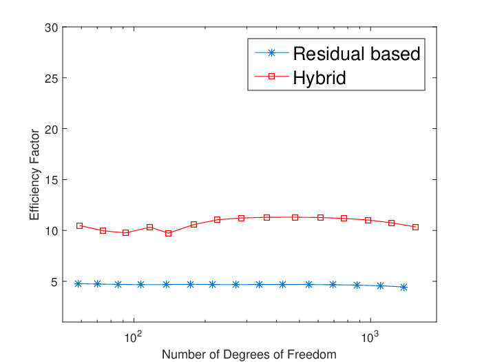
Refer to caption
Figure 3. Efficiency factors plotted against the number of degrees of freedom for two types of mesh refinements.
Refer to caption
Figure 4. Second-order derivative ratios RV1R_{V}^{1}, RV2R_{V}^{2} and RV3R_{V}^{3}.

6.2. Numerical Results

We summarize the results of the computations with meshes generated by the adaptive algorithm with both the residual based and the hybrid error estimators. In addition, we plot the ratios between the maximum and minimum values of different groups of the second-order derivatives ∂i​jV\partial_{ij}V to support the assumptions we proposed 2.3.3.

  1. (1)

    In 2 we display the relative errors for the two types of mesh generation algorithms. The differences between the results produced by the two algorithms is negligible. We observe the convergence rates close to (#​DoF)−1(\#{\rm DoF})^{-1} for both algorithms as expected.

  2. (2)

    The efficiency indicators (estimate divided by the actual error) are displayed in 3, from which we observe that both the residual based error estimator and the hybrid error estimator possess good efficiency throughout the computations. The hybrid estimator has a slightly larger efficiency factor because of the estimated constants Cz−cgC^{{\rm z}-{\rm cg}} and Cz−moC^{{\rm z}-{\rm mo}} defined in (5.38) whose actual values are difficult (if not impossible) to track.

  3. (3)

    4 displays the ratios of second-order derivatives ∂i​jV\partial_{ij}V and ∂i​jΦa\partial_{ij}\Phi^{\rm a}. In particular, we define

    RV1\displaystyle R_{V}^{1} :=infℓ∈ℒ,i=±1|∂i​iV⁡(yℓac)|/supℓ∈ℒ,(i,j)∈𝒮NNN1|∂i​jV⁡(yℓac)|,\displaystyle:=\inf_{\begin{subarray}{c}\ell\in\mathcal{L},\\ i=\pm 1\end{subarray}}|\partial_{ii}V(y^{{\rm ac}}_{\ell})|/\sup_{\begin{subarray}{c}\ell\in\mathcal{L},\\ (i,j)\in\mathcal{S}^{{\rm NNN}_{1}}\end{subarray}}|\partial_{ij}V(y^{{\rm ac}}_{\ell})|, (6.3)
    RV2\displaystyle R_{V}^{2} :=infℓ∈ℒ,(i,j)∈𝒮NNN1|∂i​iV⁡(yℓac)|/supℓ∈ℒ,(i,j)∈𝒮NNN2|∂i​jV⁡(yℓac)|,\displaystyle:=\inf_{\begin{subarray}{c}\ell\in\mathcal{L},\\ (i,j)\in\mathcal{S}^{{\rm NNN}_{1}}\end{subarray}}|\partial_{ii}V(y^{{\rm ac}}_{\ell})|/\sup_{\begin{subarray}{c}\ell\in\mathcal{L},\\ (i,j)\in\mathcal{S}^{{\rm NNN}_{2}}\end{subarray}}|\partial_{ij}V(y^{{\rm ac}}_{\ell})|, (6.4)
    RV3\displaystyle R_{V}^{3} :=infℓ∈ℒ,(i,j)∈𝒮NNN2|∂i​iV⁡(yℓac)|/supℓ∈ℒ,(i,j)∈𝒮NNN3|∂i​jV⁡(yℓac)|,\displaystyle:=\inf_{\begin{subarray}{c}\ell\in\mathcal{L},\\ (i,j)\in\mathcal{S}^{{\rm NNN}_{2}}\end{subarray}}|\partial_{ii}V(y^{{\rm ac}}_{\ell})|/\sup_{\begin{subarray}{c}\ell\in\mathcal{L},\\ (i,j)\in\mathcal{S}^{{\rm NNN}_{3}}\end{subarray}}|\partial_{ij}V(y^{{\rm ac}}_{\ell})|, (6.5)

    where where 𝒮NNN1,𝒮NNN2\mathcal{S}^{{\rm NNN}_{1}},\mathcal{S}^{{\rm NNN}_{2}} and 𝒮NNN3\mathcal{S}^{{\rm NNN}_{3}} are defined by (2.33), (2.34) and (2.35). We find that the nearest-neighbour derivatives |∂11V⁡(𝒈)||\partial_{11}V(\boldsymbol{g})| and |∂33V⁡(𝒈)||\partial_{33}V(\boldsymbol{g})| are significantly larger than other types of derivatives in terms of the absolute value which essentially reflects the nearest-neighbor dominant feature of our interaction potential.

  4. (4)

    In 4, we also test the assumption for two pair potential cases as RΦMR^{{\rm M}}_{\Phi} and RΦLJR^{{\rm LJ}}_{\Phi}, which are defined by

    RΦM:=infℓ∈ℒ,i=±1|∂i​iΦM​(yℓac)|/supℓ∈ℒ,(i,j)∈𝒮NNN1|∂i​jΦM​(yℓac)|,R_{\Phi}^{{\rm M}}:=\inf_{\begin{subarray}{c}\ell\in\mathcal{L},\\ i=\pm 1\end{subarray}}|\partial_{ii}\Phi^{{\rm M}}(y^{{\rm ac}}_{\ell})|/\sup_{\begin{subarray}{c}\ell\in\mathcal{L},\\ (i,j)\in\mathcal{S}^{{\rm NNN}_{1}}\end{subarray}}|\partial_{ij}\Phi^{{\rm M}}(y^{{\rm ac}}_{\ell})|, (6.6)

    and

    RΦLJ:=infℓ∈ℒ,i=±1|∂i​iΦLJ​(yℓac)|/supℓ∈ℒ,(i,j)∈𝒮NNN1|∂i​jΦLJ​(yℓac)|,R_{\Phi}^{{\rm LJ}}:=\inf_{\begin{subarray}{c}\ell\in\mathcal{L},\\ i=\pm 1\end{subarray}}|\partial_{ii}\Phi^{{\rm LJ}}(y^{{\rm ac}}_{\ell})|/\sup_{\begin{subarray}{c}\ell\in\mathcal{L},\\ (i,j)\in\mathcal{S}^{{\rm NNN}_{1}}\end{subarray}}|\partial_{ij}\Phi^{{\rm LJ}}(y^{{\rm ac}}_{\ell})|, (6.7)

    where ΦM\Phi^{\rm M} and ΦLJ\Phi^{\rm LJ} respectively denote Morse potential and Lennard-Jones potential. The explicit form of these two types of potential are given by

    Φℓγ​(y)=12​[ϕγ​(yℓ+1′)+ϕγ​(yℓ′)+ϕγ​(yℓ+1′+yℓ+2′)+ϕγ​(yℓ−1′+yℓ′)],γ∈{M,LJ},\Phi^{\gamma}_{\ell}(y)=\frac{1}{2}[\phi^{\gamma}(y^{\prime}_{\ell+1})+\phi^{\gamma}(y^{\prime}_{\ell})+\phi^{\gamma}(y^{\prime}_{\ell+1}+y^{\prime}_{\ell+2})+\phi^{\gamma}(y^{\prime}_{\ell-1}+y^{\prime}_{\ell})],\ \gamma\in\{{\rm M},{\rm LJ}\}, (6.8)

    and

    ϕM​(r)\displaystyle\phi^{\rm M}(r) =e−10​(r−1)−2​e−5​(r−1),\displaystyle=e^{-10(r-1)}-2e^{-5(r-1)}, (6.9)
    ϕLJ​(r)\displaystyle\phi^{\rm LJ}(r) =r−12−2​r−6.\displaystyle=r^{-12}-2r^{-6}. (6.10)

    We note that for pair potentials all the cross derivative terms vanish and only one ratio is related which is essentially equivalent to RV1R^{1}_{V} in 6.3 for the many-body case.

We can conclude that both a posteriori error indicators can be used to select meshes that are quasi-optimal at least for our model problem (also c.f. [27, Section 6 Figure 1] for the discussion of quasi-optimality).

7. Conclusion

We have derived and analyzed two different types of a posteriori error estimators for the GRAC a/c coupling method in 1D. The residual based error estimator is proved to be efficient that provides both the upper bound globally and the lower bound (up to some generic constants) locally for the true error between the solution of the coupling model and the atomistic model. Our analysis applies to generic energy-based a/c methods and interaction potentials. We then analyzed the gradient recovery type error estimator which is easy to implement and hence is widely used in computational material science and engineering community. We proved the equivalence between the residual based and (a modified) gradient recovery error estimators in the continuum region. However, in order to keep the error estimator sharp on the interface which is important in the adaptive solution of our coupling model, we combine the two types of error estimators to propose a hybrid error estimator. Our numerical experiments then indicate that both estimators give the correct convergence rate and illustrate the efficiency of the estimators.

We conclude by pointing out the merit of the extension of our analysis to higher dimensional problems. The residual based a posteriori error estimate for GRAC model in 2D has been proposed in [37] where the complexity of implementation is encountered. One particular difficulty is the implementation and the computation of the model error along each finite element boundary which requires the tracing of discrepancy of the geometry of the underline lattice and the coarse-grained mesh. However, our analysis of the efficiency of the residual based estimator and derivation of the hybrid estimator essentially imply that influence of the model error in the continuum region may be marginal compared with the coarse-graining error, especially on the large elements. We believe that similar phenomenon appears in higher dimensions and can be rigorously proved with careful (but maybe much more involved) consideration, for which our 1D analysis provides a valuable stepping-stone. Moreover, the hybrid error estimator may also be extended to higher dimensions where the effect of the interface plays much more important role in adaptivity (c.f. [37]) and can be used for more efficient but reliable application of adaptive atomistic-to-continuum coupling methods.

Appendix A Detailed Formulations by Some Symbols

A.1. Details on the deformation gradient D​yhDy^{h}

We write out the specific form of D​yhDy^{h}. Inside the continuum region where k∈𝒦̊ck\in\mathring{\mathscr{K}}^{c}, we define the deformation gradient D​yℓhDy_{\ell}^{h}, whose support index is {ℓk−1+2,…,ℓk+1}\{\ell_{k-1}+2,...,\ell_{k}+1\}, by

D​yℓh={(yh′|Tk,yh′|Tk+yh′|Tk+1,−yh′|Tk,−2​yh′|Tk),ℓ=ℓk−1,(yh′|Tk+1,2​yh′|Tk+1,−yh′|Tk,−2​yh′|Tk),ℓ=ℓk,(yh′|Tk+1,2​yh′|Tk+1,−yh′|Tk+1,−yh′|Tk−yh′|Tk+1),ℓ=ℓk+1,(yh′|Tk,2​yh′|Tk,−yh′|Tk,−2​yh′|Tk),otherwise.\displaystyle Dy_{\ell}^{h}=\left\{\begin{array}[]{l l}(y_{h}^{\prime}{}|_{T_{k}},y_{h}^{\prime}{}|_{T_{k}}+y_{h}^{\prime}{}|_{T_{k+1}},-y_{h}^{\prime}{}|_{T_{k}},-2y_{h}^{\prime}{}|_{T_{k}}),&\ell=\ell_{k}-1,\\ (y_{h}^{\prime}{}|_{T_{k+1}},2y_{h}^{\prime}{}|_{T_{k+1}},-y_{h}^{\prime}{}|_{T_{k}},-2y_{h}^{\prime}{}|_{T_{k}}),&\ell=\ell_{k},\\ (y_{h}^{\prime}{}|_{T_{k+1}},2y_{h}^{\prime}{}|_{T_{k+1}},-y_{h}^{\prime}{}|_{T_{k+1}},-y_{h}^{\prime}{}|_{T_{k}}-y_{h}^{\prime}{}|_{T_{k+1}}),&\ell=\ell_{k}+1,\\ (y_{h}^{\prime}{}|_{T_{k}},2y_{h}^{\prime}{}|_{T_{k}},-y_{h}^{\prime}{}|_{T_{k}},-2y_{h}^{\prime}{}|_{T_{k}}),&\text{otherwise}.\end{array}\right.

Around the interface, we have

D​yℓh={(yh′|TK1−1,yh′|TK1−1+yh′|TK1,−yh′|TK1−2,−2​yh′|TK1−2),ℓ=ℓK1−2,(yh′|TK2+3,2​yh′|TK2+3,−yh′|TK2+2,−yh′|TK2+1−yh′|TK2+2),ℓ=ℓK2+2.\displaystyle Dy_{\ell}^{h}=\left\{\begin{array}[]{l l}(y_{h}^{\prime}{}|_{T_{K_{1}-1}},y_{h}^{\prime}{}|_{T_{K_{1}-1}}+y_{h}^{\prime}{}|_{T_{K_{1}}},-y_{h}^{\prime}{}|_{T_{K_{1}-2}},-2y_{h}^{\prime}{}|_{T_{K_{1}-2}}),&\ell=\ell_{K_{1}-2},\\ (y_{h}^{\prime}{}|_{T_{K_{2}+3}},2y_{h}^{\prime}{}|_{T_{K_{2}+3}},-y_{h}^{\prime}{}|_{T_{K_{2}+2}},-y_{h}^{\prime}{}|_{T_{K_{2}+1}}-y_{h}^{\prime}{}|_{T_{K_{2}+2}}),&\ell=\ell_{K_{2}+2}.\end{array}\right.

Finally, for the atoms inside the atomistic region where k=K1−1,…,K2+1k=K_{1}-1,\dots,K_{2}+1, the formula of D​yhDy^{h} is simply given by

D​yℓkh=(yh′|Tk+1,yh′|Tk+1+yh′|Tk+2,−yh′|Tk,−yh′|Tk−1−yh′|Tk).Dy_{\ell_{k}}^{h}=(y_{h}^{\prime}{}|_{T_{k+1}},y_{h}^{\prime}{}|_{T_{k+1}}+y_{h}^{\prime}{}|_{T_{k+2}},-y_{h}^{\prime}{}|_{T_{k}},-y_{h}^{\prime}{}|_{T_{k-1}}-y_{h}^{\prime}{}|_{T_{k}}).

A.2. Details on the stress tensors of the coupling model σ¯ka​c​(yh)\bar{\sigma}^{ac}_{k}(y_{h})

Upon defining

∂jV−i​(D​yℓ):=∂jV⁡(D1​yℓ,D2​yℓ,D−1​yℓ,2​D−1​yℓ),\displaystyle\partial_{j}V_{-}^{i}(Dy_{\ell}):=\partial_{j}V(D_{1}y_{\ell},D_{2}y_{\ell},D_{-1}y_{\ell},2D_{-1}y_{\ell}),
∂jV+i​(D​yℓ):=∂jV⁡(D1​yℓ,2​D1​yℓ,D−1​yℓ,D−2​yℓ),\displaystyle\partial_{j}V_{+}^{i}(Dy_{\ell}):=\partial_{j}V(D_{1}y_{\ell},2D_{1}y_{\ell},D_{-1}y_{\ell},D_{-2}y_{\ell}),

the elementwise stress tensors of the coupling model σ¯ka​c​(yh)\bar{\sigma}^{ac}_{k}(y_{h}) is given by

σ¯kac​(yh)={σℓka​(yh),k∈𝒦~a,W′​(yh′|Tk),k∈𝒦~c,12​W′​(yh′|Tk)−∂−1V−i​(D​yℓkh)−2​∂−2V−i​(D​yℓkh),k=K1−1,∂1V−i​(D​yℓk−1h)−∂−1V−i​(D​yℓkh)+∂2Vi−(Dyhℓk−1)−2∂−2Vi−(Dyhℓk)−∂−2V(Dyhℓk+1),k=K1,∂1V−i​(D​yℓk−1h)−∂−1V⁡(D​yℓkh)+∂2V−i​(D​yℓk−2h)+∂2Vi−(Dyhℓk−1)−∂−2V(Dyhℓk)−∂−2V(Dyhℓk+1),k=K1+1,∂1V⁡(D​yℓk−1h)−∂−1V⁡(D​yℓkh)+∂2V−i​(D​yℓk−2h)+∂2V(Dyhℓk−1)−∂−2V(Dyhℓk)−∂−2V(Dyhℓk+1),k=K1+2,∂1V⁡(D​yℓk−1h)−∂−1V⁡(D​yℓkh)+∂2V⁡(D​yℓk−1h)+∂2V(Dyhℓk−2)−∂−2V(Dyhℓk)−∂−2V+i(Dyhℓk+1),k=K2−1,∂1V⁡(D​yℓk−1h)−∂−1V+i​(D​yℓkh)+∂2V⁡(D​yℓk−1h)+∂2V(Dyhℓk−2)−∂−2V+i(Dyhℓk)−∂−2V+i(Dyhℓk+1),k=K2,∂1V+i​(D​yℓk−1h)−∂−1V+i​(D​yℓkh)+∂2V(Dyhℓk−2)+2∂2V+i(Dyhℓk−1)−∂−2V+i(Dyhℓk),k=K2+1,12​W′​(yh′|Tk)+∂1V+i​(D​yℓk−1h)+2​∂2V+i​(D​yℓk−1h),k=K2+2.\displaystyle\bar{\sigma}^{{\rm ac}}_{k}(y_{h})=\left\{\begin{array}[]{l l}\sigma^{{\rm a}}_{\ell_{k}}(y_{h}),&k\in\widetilde{\mathscr{K}}^{a},\\ W^{\prime}(y_{h}^{\prime}{}|_{T_{k}}),&k\in\widetilde{\mathscr{K}}^{c},\\ \frac{1}{2}W^{\prime}(y_{h}^{\prime}{}|_{T_{k}})-\partial_{-1}V^{i}_{-}(Dy^{h}_{\ell_{k}})-2\partial_{-2}V^{i}_{-}(Dy^{h}_{\ell_{k}}),&k=K_{1}-1,\\ \partial_{1}V^{i}_{-}(Dy^{h}_{\ell_{k-1}})-\partial_{-1}V^{i}_{-}(Dy^{h}_{\ell_{k}})\\ +\partial_{2}V^{i}_{-}(Dy^{h}_{\ell_{k-1}})-2\partial_{-2}V^{i}_{-}(Dy^{h}_{\ell_{k}})-\partial_{-2}V(Dy^{h}_{\ell_{k+1}}),&k=K_{1},\\ \partial_{1}V^{i}_{-}(Dy^{h}_{\ell_{k-1}})-\partial_{-1}V(Dy^{h}_{\ell_{k}})+\partial_{2}V^{i}_{-}(Dy^{h}_{\ell_{k-2}})\\ +\partial_{2}V^{i}_{-}(Dy^{h}_{\ell_{k-1}})-\partial_{-2}V(Dy^{h}_{\ell_{k}})-\partial_{-2}V(Dy^{h}_{\ell_{k+1}}),&k=K_{1}+1,\\ \partial_{1}V(Dy^{h}_{\ell_{k-1}})-\partial_{-1}V(Dy^{h}_{\ell_{k}})+\partial_{2}V^{i}_{-}(Dy^{h}_{\ell_{k-2}})\\ +\partial_{2}V(Dy^{h}_{\ell_{k-1}})-\partial_{-2}V(Dy^{h}_{\ell_{k}})-\partial_{-2}V(Dy^{h}_{\ell_{k+1}}),&k=K_{1}+2,\\ \partial_{1}V(Dy^{h}_{\ell_{k-1}})-\partial_{-1}V(Dy^{h}_{\ell_{k}})+\partial_{2}V(Dy^{h}_{\ell_{k-1}})\\ +\partial_{2}V(Dy^{h}_{\ell_{k-2}})-\partial_{-2}V(Dy^{h}_{\ell_{k}})-\partial_{-2}V^{+}_{i}(Dy^{h}_{\ell_{k+1}}),&k=K_{2}-1,\\ \partial_{1}V(Dy^{h}_{\ell_{k-1}})-\partial_{-1}V_{+}^{i}(Dy^{h}_{\ell_{k}})+\partial_{2}V(Dy^{h}_{\ell_{k-1}})\\ +\partial_{2}V(Dy^{h}_{\ell_{k-2}})-\partial_{-2}V_{+}^{i}(Dy^{h}_{\ell_{k}})-\partial_{-2}V_{+}^{i}(Dy^{h}_{\ell_{k+1}}),&k=K_{2},\\ \partial_{1}V_{+}^{i}(Dy^{h}_{\ell_{k-1}})-\partial_{-1}V_{+}^{i}(Dy^{h}_{\ell_{k}})\\ +\partial_{2}V(Dy^{h}_{\ell_{k-2}})+2\partial_{2}V_{+}^{i}(Dy^{h}_{\ell_{k-1}})-\partial_{-2}V_{+}^{i}(Dy^{h}_{\ell_{k}}),&k=K_{2}+1,\\ \frac{1}{2}W^{\prime}(y_{h}^{\prime}{}|_{T_{k}})+\partial_{1}V^{i}_{+}(Dy^{h}_{\ell_{k-1}})+2\partial_{2}V^{i}_{+}(Dy^{h}_{\ell_{k-1}}),&k=K_{2}+2.\end{array}\right.

where F→:=(F,2​F,−F,−2​F)\vec{F}:=(F,2F,-F,-2F), W′​(F):=∑j=±1(−1)j−12​[∂jV⁡(F→)+2​∂2×jV⁡(F→)]W^{\prime}(F):=\sum_{j=\pm 1}(-1)^{\frac{j-1}{2}}[\partial_{j}V(\vec{F})+2\partial_{2\times j}V(\vec{F})] and σℓka​(yh)\sigma^{{\rm a}}_{\ell_{k}}(y_{h}) is given in (2.8).

Appendix B Proofs for Some Auxiliary Results

B.1. Proof for propositions (4.5)(4.6)(4.7)

Here, we give the proof for the two propositions (4.5)(4.6)(4.7) and estimate the values of C1C_{1}, C2C_{2} and C3C_{3}.

Proof.

In the following proof, we use the symbols ℓ1k=ℓk−1+3\ell^{k}_{1}=\ell_{k-1}+3 and ℓ2k=ℓk−3\ell^{k}_{2}=\ell_{k}-3 for simplification.

For proposition (4.5). We can compute the discrete derivative bℓTk′{b^{T_{k}}_{\ell}}^{\prime} as

bℓTk′={4hTk2​(x1k+x2k+ε−2​ε​ℓ),ℓ=ℓ1k+1,…,ℓ2k,0, otherwise .\displaystyle{b^{T_{k}}_{\ell}}^{\prime}=\left\{\begin{array}[]{l l}\frac{4}{h_{T_{k}}^{2}}(x_{1}^{k}+x_{2}^{k}+\varepsilon-2\varepsilon\ell),&\ell=\ell^{k}_{1}+1,\dots,\ell^{k}_{2},\\ 0,&\text{ otherwise }.\end{array}\right.

Therefore, we have

‖bTk′‖ℓε2​(ℒ̊Tk)2=16​ε3h̊Tk4​∑ℓ=ℓ1k+1ℓ2k[4​ℓ2+4​(ℓ1k+ℓ2k+1)​ℓ+(ℓ1k+ℓ2k+1)2].\|{b^{T_{k}}}^{\prime}\|^{2}_{\ell_{\varepsilon}^{2}(\mathring{\mathcal{L}}_{T_{k}})}=\frac{16\varepsilon^{3}}{\mathring{h}^{4}_{T_{k}}}\sum_{\ell=\ell^{k}_{1}+1}^{\ell^{k}_{2}}[4\ell^{2}+4(\ell^{k}_{1}+\ell^{k}_{2}+1)\ell+(\ell^{k}_{1}+\ell^{k}_{2}+1)^{2}]. (B.1)

Apply the following facts:

∑i=1ni=\displaystyle\sum_{i=1}^{n}i= i⁡(i+1)2;\displaystyle\frac{i(i+1)}{2}; (B.2)
∑i=1ni2=\displaystyle\sum_{i=1}^{n}i^{2}= i​(i+1)​(2​i+1)6,\displaystyle\frac{i(i+1)(2i+1)}{6}, (B.3)

and then we have

‖bTk′‖ℓε2​(ℒ̊Tk)2=163​[1−(εh̊Tk)2]​hTk−1,\|{b^{T_{k}}}^{\prime}\|^{2}_{\ell_{\varepsilon}^{2}(\mathring{\mathcal{L}}_{T_{k}})}=\frac{16}{3}[1-(\frac{\varepsilon}{\mathring{h}_{T_{k}}})^{2}]h^{-1}_{T_{k}}, (B.4)

which leads us to the result (4.5).

For proposition (4.6). Similarly we compute

‖bTk‖ℓε2​(ℒ̊Tk)2=16​ε5h̊Tk4​∑ℓ=ℓ1k+1ℓ2k{ℓ4−2​(ℓ1k+ℓ2k)​ℓ3+[(ℓ1k)2+4​ℓ1k​ℓ2k+(ℓ2k)2]​ℓ2−2​ℓ1k​ℓ2k​(ℓ1k+ℓ2k)​ℓ+(ℓ1k)2​(ℓ2k)2}.\|b^{T_{k}}\|^{2}_{\ell_{\varepsilon}^{2}(\mathring{\mathcal{L}}_{T_{k}})}=\frac{16\varepsilon^{5}}{\mathring{h}_{T_{k}}^{4}}\sum_{\ell=\ell^{k}_{1}+1}^{\ell^{k}_{2}}\{\ell^{4}-2(\ell^{k}_{1}+\ell^{k}_{2})\ell^{3}+[(\ell^{k}_{1})^{2}+4\ell^{k}_{1}\ell^{k}_{2}+(\ell^{k}_{2})^{2}]\ell^{2}-2\ell^{k}_{1}\ell^{k}_{2}(\ell^{k}_{1}+\ell^{k}_{2})\ell+(\ell^{k}_{1})^{2}(\ell^{k}_{2})^{2}\}. (B.5)

By the facts

∑i=1ni3=\displaystyle\sum_{i=1}^{n}i^{3}= 14​i2​(i+1)2;\displaystyle\frac{1}{4}i^{2}(i+1)^{2}; (B.6)
∑i=1ni4=\displaystyle\sum_{i=1}^{n}i^{4}= i⁡(i+1)​(2​i+1)​(3​i2+3​i−1)30,\displaystyle\frac{i(i+1)(2i+1)(3i^{2}+3i-1)}{30}, (B.7)

together with (B.2) and (B.3), we have

‖bTk′‖ℓε2​(ℒ̊Tk)2=815​[1−(εh̊Tk)4]​h̊Tk,\|{b^{T_{k}}}^{\prime}\|^{2}_{\ell_{\varepsilon}^{2}(\mathring{\mathcal{L}}_{T_{k}})}=\frac{8}{15}[1-(\frac{\varepsilon}{\mathring{h}_{T_{k}}})^{4}]\mathring{h}_{T_{k}}, (B.8)

and the result (4.6) can then be directly obtained by taking square root on both sides of the equation above.

For proposition (4.7). We directly calculate that

ε​∑ℓ=ℓ1k+1ℓ2kbℓTk=4​ε3h̊Tk2​∑ℓ=ℓ1k+1ℓ2k[−ℓ2+(ℓ1k+ℓ2k)​ℓ−ℓ1k​ℓ2k].\varepsilon\sum_{\ell=\ell^{k}_{1}+1}^{\ell^{k}_{2}}b^{T_{k}}_{\ell}=\frac{4\varepsilon^{3}}{\mathring{h}^{2}_{T_{k}}}\sum_{\ell=\ell^{k}_{1}+1}^{\ell^{k}_{2}}[-\ell^{2}+(\ell^{k}_{1}+\ell^{k}_{2})\ell-\ell^{k}_{1}\ell^{k}_{2}]. (B.9)

Again by (B.2) and (B.3), we have

ε​∑ℓ=ℓ1k+1ℓ2kbℓTk=23​[1−(εh̊Tk)2]​h̊Tk,\varepsilon\sum_{\ell=\ell^{k}_{1}+1}^{\ell^{k}_{2}}b^{T_{k}}_{\ell}=\frac{2}{3}[1-(\frac{\varepsilon}{\mathring{h}_{T_{k}}})^{2}]\mathring{h}_{T_{k}}, (B.10)

which gives us proposition (4.7). ∎

B.2. Proof for (2.21)

Proof.

We write the inner product ⟨f,yh⟩ε\langle f,y_{h}\rangle_{\varepsilon} as

⟨f,yh⟩ε=ε​∑ℓ∈𝒞\{ℓK2+2}fℓ​yℓh+ε​∑ℓ=ℓK1−1ℓK2+2fℓ​yℓh,\langle f,y_{h}\rangle_{\varepsilon}=\varepsilon\sum_{\ell\in\mathcal{C}\backslash\{\ell_{K_{2}+2}\}}f_{\ell}y^{h}_{\ell}+\varepsilon\sum_{\ell=\ell_{K_{1}-1}}^{\ell_{K_{2}+2}}f_{\ell}y^{h}_{\ell}, (B.11)

where

ε​∑ℓ∈𝒞\{ℓK2+2}fℓ​yℓh\displaystyle\varepsilon\sum_{\ell\in\mathcal{C}\backslash\{\ell_{K_{2}+2}\}}f_{\ell}y^{h}_{\ell}
=\displaystyle= ε​∑k∈𝒦c\{K2+2}∑ℓ∈ℒTk[yℓk−1+yℓk−yℓk−1hTk​(ℓ−ℓk−1)​ε]​fℓ\displaystyle\varepsilon\sum_{k\in\mathscr{K}^{c}\backslash\{K_{2}+2\}}\sum_{\ell\in\mathcal{L}_{T_{k}}}[y_{\ell_{k-1}}+\frac{y_{\ell_{k}}-y_{\ell_{k-1}}}{h_{T_{k}}}(\ell-\ell_{k-1})\varepsilon]f_{\ell}
=\displaystyle= ε​∑k∈𝒦c\{K2+2}∑ℓ∈ℒTkℓ−ℓk−1hTk​ε​fℓ​yℓk+ε​∑k∈𝒦c\{K2+2}∑ℓ∈ℒTk+1(1−ℓ−ℓkhTk+1​ε)​fℓ​yℓk\displaystyle\varepsilon\sum_{k\in\mathscr{K}^{c}\backslash\{K_{2}+2\}}\sum_{\ell\in\mathcal{L}_{T_{k}}}\frac{\ell-\ell_{k-1}}{h_{T_{k}}}\varepsilon f_{\ell}y_{\ell_{k}}+\varepsilon\sum_{k\in\mathscr{K}^{c}\backslash\{K_{2}+2\}}\sum_{\ell\in\mathcal{L}_{T_{k+1}}}(1-\frac{\ell-\ell_{k}}{h_{T_{k+1}}}\varepsilon)f_{\ell}y_{\ell_{k}}
=\displaystyle= ε​∑k∈𝒦̊c{ε​∑ℓ∈ℒTkℓ−ℓk−1hTk​ε​fℓ+∑ℓ∈ℒTk+1(1−ℓ−ℓkhTk+1​ε)​fℓ}​yℓk\displaystyle\varepsilon\sum_{k\in\mathring{\mathscr{K}}^{c}}\big\{\varepsilon\sum_{\ell\in\mathcal{L}_{T_{k}}}\frac{\ell-\ell_{k-1}}{h_{T_{k}}}\varepsilon f_{\ell}+\sum_{\ell\in\mathcal{L}_{T_{k+1}}}(1-\frac{\ell-\ell_{k}}{h_{T_{k+1}}}\varepsilon)f_{\ell}\big\}y_{\ell_{k}}
+\displaystyle+ ε​∑ℓ∈ℒTK1−2ℓ−ℓK1−3hK1−2​ε​fℓ​yℓK1−2+ε​∑ℓ∈ℒTK2+3(1−ℓ−ℓK2+2hK2+3​ε)​fℓ​yℓK2+2,\displaystyle\varepsilon\sum_{\ell\in\mathcal{L}_{T_{K_{1}-2}}}\frac{\ell-\ell_{K_{1}-3}}{h_{K_{1}-2}}\varepsilon f_{\ell}y_{\ell_{K_{1}-2}}+\varepsilon\sum_{\ell\in\mathcal{L}_{T_{K_{2}+3}}}(1-\frac{\ell-\ell_{K_{2}+2}}{h_{K_{2}+3}}\varepsilon)f_{\ell}y_{\ell_{K_{2}+2}}, (B.12)

and

ε​∑ℓ=ℓK1−1ℓK2+2fℓ​yℓh=ε​∑k=K1−1K2+2fℓk​yℓkh.\varepsilon\sum_{\ell=\ell_{K_{1}-1}}^{\ell_{K_{2}+2}}f_{\ell}y^{h}_{\ell}=\varepsilon\sum_{k=K_{1}-1}^{K_{2}+2}f_{\ell_{k}}y^{h}_{\ell_{k}}. (B.13)

Combining (B.12) and (B.13), we can write (B.11) into the form of

⟨f,yh⟩ε=∑k∈𝒦a​cε​f¯k​yℓkh,\langle f,y_{h}\rangle_{\varepsilon}=\sum_{k\in\mathscr{K}^{ac}}\varepsilon\bar{f}_{k}y^{h}_{\ell_{k}},

where the projected force f¯k\bar{f}_{k} has been given in (2.21).

∎

B.3. Proof for (5.12)

Proof.

To prove (5.12), we only need to show that: for any vh∈𝒰hv_{h}\in\mathcal{U}^{h}, we have

(vh,vh)h∼‖vh‖ℓε2​(𝒞∪ℐ\{ℓK2})2.(v_{h},v_{h})_{h}\sim\|v_{h}\|^{2}_{\ell^{2}_{\varepsilon}(\mathcal{C}\cup\mathcal{I}\backslash\{\ell_{K_{2}}\})}. (B.14)

The right part of (B.14) can be easily computed as

‖vh‖ℓε2​(𝒞∪ℐ\{ℓK2})2=AN+BN,\|v_{h}\|^{2}_{\ell^{2}_{\varepsilon}(\mathcal{C}\cup\mathcal{I}\backslash\{\ell_{K_{2}}\})}=A^{N}+B^{N},

where

AN:=\displaystyle A^{N}:= ∑k∈𝒦𝒯hc{hTk3​[(vℓkh)2+vℓkh​vℓk−1h+(vℓk−1h)2]+ε2​[(vℓkh)2−(vℓk−1h)2]+ε23​hTk​[vℓkh−vℓk−1h]2},\displaystyle\sum_{k\in\mathscr{K}_{\mathscr{T}_{h}}^{c}}\big\{\frac{h_{T_{k}}}{3}[(v^{h}_{\ell_{k}})^{2}+v^{h}_{\ell_{k}}v^{h}_{\ell_{k-1}}+(v^{h}_{\ell_{k-1}})^{2}]+\frac{\varepsilon}{2}[(v^{h}_{\ell_{k}})^{2}-(v^{h}_{\ell_{k-1}})^{2}]+\frac{\varepsilon^{2}}{3h_{T_{k}}}[v^{h}_{\ell_{k}}-v^{h}_{\ell_{k-1}}]^{2}\big\},
BN:=\displaystyle B^{N}:= ε2​∑k∈{K1−2,K2+2}(vℓkh)2+ε​∑k∈{K1−1,K2+1}(vℓkh)2,\displaystyle\frac{\varepsilon}{2}\sum_{k\in\{K_{1}-2,K_{2}+2\}}(v^{h}_{\ell_{k}})^{2}+\varepsilon\sum_{k\in\{K_{1}-1,K_{2}+1\}}(v^{h}_{\ell_{k}})^{2},

while the left part

(vh,vh)h=AI​P+BI​P,(v_{h},v_{h})_{h}=A^{IP}+B^{IP},

where

AI​P:=\displaystyle A^{IP}:= 12​∑k∈𝒦𝒯hchTk​[(vℓkh)2+(vℓk−1h)2],\displaystyle\frac{1}{2}\sum_{k\in\mathscr{K}_{\mathscr{T}_{h}}^{c}}h_{T_{k}}[(v^{h}_{\ell_{k}})^{2}+(v^{h}_{\ell_{k-1}})^{2}],
BI​P:=\displaystyle B^{IP}:= ε2​∑k∈{K1−2,K1−1,K2+1,K2+2}(vℓkh)2.\displaystyle\frac{\varepsilon}{2}\sum_{k\in\{K_{1}-2,K_{1}-1,K_{2}+1,K_{2}+2\}}(v^{h}_{\ell_{k}})^{2}.

By using the fact that hTk≥εh_{T_{k}}\geq\varepsilon and the mean value inequality, we have

AN≤\displaystyle A^{N}\leq 12​∑k∈𝒦𝒯hc(hTk+ε23​hTk)​[(vℓkh)2+(vℓk−1h)2]\displaystyle\frac{1}{2}\sum_{k\in\mathscr{K}_{\mathscr{T}_{h}}^{c}}(h_{T_{k}}+\frac{\varepsilon^{2}}{3h_{T_{k}}})[(v^{h}_{\ell_{k}})^{2}+(v^{h}_{\ell_{k-1}})^{2}]
≤\displaystyle\leq 23​∑k∈𝒦𝒯hchTk​[(vℓkh)2+(vℓk−1h)2]=43​AI​P\displaystyle\frac{2}{3}\sum_{k\in\mathscr{K}_{\mathscr{T}_{h}}^{c}}h_{T_{k}}[(v^{h}_{\ell_{k}})^{2}+(v^{h}_{\ell_{k-1}})^{2}]=\frac{4}{3}A^{IP} (B.15)

and

AN≥16​∑k∈𝒦𝒯hchTk​[(vℓkh)2+(vℓk−1h)2]=13​AI​P.A^{N}\geq\frac{1}{6}\sum_{k\in\mathscr{K}_{\mathscr{T}_{h}}^{c}}h_{T_{k}}[(v^{h}_{\ell_{k}})^{2}+(v^{h}_{\ell_{k-1}})^{2}]=\frac{1}{3}A^{IP}. (B.16)

Combining (B.15) with (B.16), we have

34​AN≤AI​P≤3​AN.\frac{3}{4}A^{N}\leq A^{IP}\leq 3A^{N}.

On the other hand, it is straightforward that

12​BN≤BI​P≤BN.\frac{1}{2}B^{N}\leq B^{IP}\leq B^{N}.

Therefore, we obtain the equivalence as

12​‖vh‖ℓε2​(𝒞∪ℐ\{ℓK2})2≤(vh,vh)h≤3​‖vh‖ℓε2​(𝒞∪ℐ\{ℓK2})2\frac{1}{2}\|v_{h}\|^{2}_{\ell^{2}_{\varepsilon}(\mathcal{C}\cup\mathcal{I}\backslash\{\ell_{K_{2}}\})}\leq(v_{h},v_{h})_{h}\leq 3\|v_{h}\|^{2}_{\ell^{2}_{\varepsilon}(\mathcal{C}\cup\mathcal{I}\backslash\{\ell_{K_{2}}\})}

∎

B.4. Proof for the interface case in lemma 5.2

Proof.

By the definition of σK1−2ac​(yac)\sigma^{{\rm ac}}_{K_{1}-2}(y_{{\rm ac}}) and σK1−1ac​(yac)\sigma^{{\rm ac}}_{K_{1}-1}(y_{{\rm ac}}) and the mean value theorem, we have

σK1−2ac(yac)−σK1−1ac(yac)=[12W′′(ξK1−2)+∂−1,−1V(ζ→−1,−1)−∂−1,1V(ζ→−1,1)\displaystyle\sigma^{{\rm ac}}_{K_{1}-2}(y_{{\rm ac}})-\sigma^{{\rm ac}}_{K_{1}-1}(y_{{\rm ac}})=[\frac{1}{2}W^{\prime\prime}(\xi_{K_{1}-2})+\partial_{-1,-1}V(\vec{\zeta}_{-1,-1})-\partial_{-1,1}V(\vec{\zeta}_{-1,1})
−2∂−1,2V(ζ→−1,2)+∂−1,−2V(ζ→−1,−2)−2∂−2,1V(ζ→−2,1)−4∂−2,2V(ζ→−2,2)+2∂−2,−1V(ζ→−2,−1)\displaystyle-2\partial_{-1,2}V(\vec{\zeta}_{-1,2})+\partial_{-1,-2}V(\vec{\zeta}_{-1,-2})-2\partial_{-2,1}V(\vec{\zeta}_{-2,1})-4\partial_{-2,2}V(\vec{\zeta}_{-2,2})+2\partial_{-2,-1}V(\vec{\zeta}_{-2,-1})
+2∂−2,−2V(ζ→−2,−2)](yh′|TK1−2−yh′|TK1−1)+[−∂−1,1V(ζ→−1,1)−2∂−1,2V(ζ→−1,2)\displaystyle+2\partial_{-2,-2}V(\vec{\zeta}_{-2,-2})](y_{h}^{\prime}|_{T_{K_{1}-2}}-y_{h}^{\prime}|_{T_{K_{1}-1}})+[-\partial_{-1,1}V(\vec{\zeta}_{-1,1})-2\partial_{-1,2}V(\vec{\zeta}_{-1,2})
−2∂−2,1V(ζ→−2,1)−4∂−2,2V(ζ→−2,2)](yh′|TK1−1−yh′|TK1)\displaystyle-2\partial_{-2,1}V(\vec{\zeta}_{-2,1})-4\partial_{-2,2}V(\vec{\zeta}_{-2,2})](y_{h}^{\prime}|_{T_{K_{1}-1}}-y_{h}^{\prime}|_{T_{K_{1}}})
+[−∂−1,2V(ζ→−1​,​2)−2∂−2,2V(ζ→−2,2)](yh′|TK1−yh′|TK1+1),\displaystyle+[-\partial_{-1,2}V(\vec{\zeta}_{-1,2})-2\partial_{-2,2}V(\vec{\zeta}_{-2,2})](y_{h}^{\prime}|_{T_{K_{1}}}-y_{h}^{\prime}|_{T_{K_{1}+1}}), (B.17)

where ξK1−2,(ζi​j)m∈⋃k∈{K1−2,K1−1,K1}conv⁡(∇yh|Tk,∇yh|Tk+1)\xi_{K_{1}-2},(\zeta_{ij})_{m}\in\bigcup_{k\in\{K_{1}-2,K_{1}-1,K_{1}\}}{\rm conv}(\nabla y_{h}|_{T_{k}},\nabla y_{h}|_{T_{k+1}}). Now we apply the assumption 2.3.3 and by the similar analysis as that in the proof for lemma 5.2, we obtain

94​[∂1,1V⁡(ξ¯→K1−2)+∂3,3V⁡(ξ¯→K1−2)]2​(ηK1−2z)2\displaystyle\frac{9}{4}[\partial_{1,1}V(\vec{\underline{\xi}}_{K_{1}-2})+\partial_{3,3}V(\vec{\underline{\xi}}_{K_{1}-2})]^{2}(\eta^{{\rm z}}_{K_{1}-2})^{2} ≤h~K1−2​|σK1−2ac​(yac)−σK1−1a​c​(yac)|2\displaystyle\leq\widetilde{h}_{K_{1}-2}|\sigma^{{\rm ac}}_{K_{1}-2}(y_{{\rm ac}})-\sigma_{K_{1}-1}^{ac}(y_{{\rm ac}})|^{2}
≤\displaystyle\leq (5​κ4​κ−2)2​[∂1,1V⁡(ξ¯→K1−2)+∂3,3V⁡(ξ¯→K1−2)]2​(ηK1−2z)2.\displaystyle(\frac{5\kappa}{4\kappa-2})^{2}[\partial_{1,1}V(\vec{\underline{\xi}}_{K_{1}-2})+\partial_{3,3}V(\vec{\underline{\xi}}_{K_{1}-2})]^{2}(\eta^{{\rm z}}_{K_{1}-2})^{2}. (B.18)

Note that here ∂1,1V⁡(ξ¯→K1−2)+∂3,3V⁡(ξ¯→K1−2)>0\partial_{1,1}V(\vec{\underline{\xi}}_{K_{1}-2})+\partial_{3,3}V(\vec{\underline{\xi}}_{K_{1}-2})>0 by (2.38). Again we apply the assumption 2.3.3, then we observe that the equivalence (5.27) still holds when k=K1−2k=K_{1}-2.

The analysis for the interface case k=K2+2k=K_{2}+2 is almost same and thus we omit its proof here. ∎

B.5. Proof for the statement in Remark 5.2

We show that the oscillated term hTk​‖f−f¯Tk‖ℓε2​(ℒTk)h_{T_{k}}\|f-\bar{f}_{T_{k}}\|_{\ell^{2}_{\varepsilon}(\mathcal{L}_{T_{k}})} and h~Tk​‖f−f¯ω~k‖ℓε2​(ℒω~k)\widetilde{h}_{T_{k}}\|f-\bar{f}_{\widetilde{\omega}_{k}}\|_{{\ell^{2}_{\varepsilon}}(\mathcal{L}_{\widetilde{\omega}_{k}})} are both high-order compared with ηcg\eta_{{\rm cg}}, where f¯Tk:=sgn⁡(f|Tk)​‖f‖L2​(Tk)hTk\bar{f}_{T_{k}}:={\rm sgn}(f|_{T_{k}})\frac{\|f\|_{L^{2}(T_{k})}}{\sqrt{h_{T_{k}}}} and the definition of f¯ω~k\bar{f}_{\widetilde{\omega}_{k}} has been given in lemma 5.2.

Proof.

For the term hTk2​‖f−f¯Tk‖ℓε2​(ℒTk)2h_{T_{k}}^{2}\|f-\bar{f}_{T_{k}}\|^{2}_{\ell^{2}_{\varepsilon}(\mathcal{L}_{T_{k}})}.

We first consider the case where f>0f>0 and thus f¯Tk>0\bar{f}_{T_{k}}>0 by its definition. Upon introducing eℓ:=|fℓ−f¯Tk|e_{\ell}:=|f_{\ell}-\bar{f}_{T_{k}}|, we have

f¯Tk​eℓ≤eℓ​(fℓ+f¯Tk)=|fℓ2−fTk2|=1hTk​|∫Tk(fℓ2−f2)​𝑑x|.\bar{f}_{T_{k}}e_{\ell}\leq e_{\ell}(f_{\ell}+\bar{f}_{T_{k}})=|f^{2}_{\ell}-f^{2}_{T_{k}}|=\frac{1}{h_{T_{k}}}|\int_{T_{k}}(f^{2}_{\ell}-f^{2})dx|. (B.19)

Now, we expand f⁡(x)f(x) at the point (ε​ℓk−1+ε​j)(\varepsilon\ell_{k-1}+\varepsilon j):

f⁡(x)=fℓk−1+j+f′​(ξ(j))​[x−(ε​ℓk−1+ε​j)]​ for some ​ξ(j)∈Tk,f(x)=f_{\ell_{k-1}+j}+f^{\prime}(\xi^{(j)})[x-(\varepsilon\ell_{k-1}+\varepsilon j)]\text{~for some~}\xi^{(j)}\in T_{k},

which is immediately followed by

1hTk​|∫Tk(fℓk−1+j2−f2)​𝑑x|=\displaystyle\frac{1}{h_{T_{k}}}|\int_{T_{k}}(f^{2}_{\ell_{k-1}+j}-f^{2})dx|= |f′​(η1(j))​fℓk−1+j​(hTk−2​ε​j)+13​[f′​(η2(j))]2​(hk2−3​ε​j​hTk+3​ε2​j2)|\displaystyle|f^{\prime}(\eta_{1}^{(j)})f_{\ell_{k-1}+j}(h_{T_{k}}-2\varepsilon j)+\frac{1}{3}[f^{\prime}(\eta_{2}^{(j)})]^{2}(h^{2}_{k}-3\varepsilon jh_{T_{k}}+3\varepsilon^{2}j^{2})|
≤\displaystyle\leq Mk2​(|hTk−2​ε​j|+13​|hk2−3​ε​j​hTk+3​ε2​j2|)\displaystyle M_{k}^{2}(|h_{T_{k}}-2\varepsilon j|+\frac{1}{3}|h^{2}_{k}-3\varepsilon jh_{T_{k}}+3\varepsilon^{2}j^{2}|)

for j=1,2,…,|ℒTk|j=1,2,\dots,|\mathcal{L}_{T_{k}}|, where η1(j),η2(j)∈Tk\eta^{(j)}_{1},\eta^{(j)}_{2}\in T_{k} and Mk:=max⁡{maxy∈Tk⁡|f⁡(y)|,maxy∈Tk⁡|f′​(y)|}M_{k}:=\max\{\max_{y\in T_{k}}|f(y)|,\max_{y\in T_{k}}|f^{\prime}(y)|\}. It is easy to check that |hTk−2​ε​j|≤hTk|h_{T_{k}}-2\varepsilon j|\leq h_{T_{k}} and 14​hk2≤|hk2−3​ε​j​hTk+3​ε2​j2|≤hk2\frac{1}{4}h^{2}_{k}\leq|h^{2}_{k}-3\varepsilon jh_{T_{k}}+3\varepsilon^{2}j^{2}|\leq h^{2}_{k}, thus we further have

1hTk​|∫Tk(fℓk−1+j2−f2)​𝑑x|≤Mk2​(13​hk2+hTk).\frac{1}{h_{T_{k}}}|\int_{T_{k}}(f^{2}_{\ell_{k-1}+j}-f^{2})dx|\leq M^{2}_{k}(\frac{1}{3}h^{2}_{k}+h_{T_{k}}). (B.20)

Plugging (B.20) into (B.19) will give us

eℓk−1+j≤Mk2f¯Tk​(13​hk2+hTk)e_{\ell_{k-1}+j}\leq\frac{M^{2}_{k}}{\bar{f}_{T_{k}}}(\frac{1}{3}h^{2}_{k}+h_{T_{k}})

and therefore the oscillated term hTk2​‖f−f¯Tk‖ℓε2​(ℒTk)2h_{T_{k}}^{2}\|f-\bar{f}_{T_{k}}\|^{2}_{\ell^{2}_{\varepsilon}(\mathcal{L}_{T_{k}})} is indeed a high-order term compared with (ηTkcg)2=12​hk3​(f¯Tk)2(\eta^{\rm cg}_{T_{k}})^{2}=\frac{1}{2}h^{3}_{k}(\bar{f}_{T_{k}})^{2} since

hTk2​‖f−f¯Tk‖ℓε2​(ℒTk)2=hk2​ε​∑j=1|ℒTk|eℓk−1+j2≤(Mk2f¯Tk)2​(hTk5+23​hk6+19​hk7).h_{T_{k}}^{2}\|f-\bar{f}_{T_{k}}\|^{2}_{\ell^{2}_{\varepsilon}(\mathcal{L}_{T_{k}})}=h^{2}_{k}\varepsilon\sum^{|\mathcal{L}_{T_{k}}|}_{j=1}e^{2}_{\ell_{k-1}+j}\leq(\frac{M^{2}_{k}}{\bar{f}_{T_{k}}})^{2}(h_{T_{k}}^{5}+\frac{2}{3}h^{6}_{k}+\frac{1}{9}h^{7}_{k}).

We omit the proof for the case f<0f<0 where we simply apply the similar analysis, then we can reach to the conclusion that hTk2​‖f−f¯Tk‖ℓε2​(ℒTk)2∼o⁡((ηTkcg)2)h_{T_{k}}^{2}\|f-\bar{f}_{T_{k}}\|^{2}_{\ell^{2}_{\varepsilon}(\mathcal{L}_{T_{k}})}\sim o((\eta^{\rm cg}_{T_{k}})^{2}).

For the term h~Tk2​‖f−f¯ω~k‖ℓε2​(ℒω~k)2\widetilde{h}_{T_{k}}^{2}\|f-\bar{f}_{\widetilde{\omega}_{k}}\|^{2}_{{\ell^{2}_{\varepsilon}}(\mathcal{L}_{\widetilde{\omega}_{k}})}.

We consider k∈𝒦c\{K}k\in\mathscr{K}^{c}\backslash\{K\}, that is, we do not consider the node on the periodic boundary of the chain. In this way, sgn⁡(f¯Tk)=sgn⁡(f¯Tk+1)=sgn⁡(f|ω~k){\rm sgn}(\bar{f}_{T_{k}})={\rm sgn}(\bar{f}_{T_{k+1}})={\rm sgn}(f|_{\tilde{\omega}_{k}}).

Due to the fact that the formula of f¯ω~k\bar{f}_{\widetilde{\omega}_{k}} inside the continuum region is different from that near the interface, we first given the proof for k∈𝒦̊ck\in\mathring{\mathscr{K}}^{c}. Similar as the analysis for the oscillated term hTk2​‖f−f¯Tk‖ℓε2​(ℒTk)2h_{T_{k}}^{2}\|f-\bar{f}_{T_{k}}\|^{2}_{\ell^{2}_{\varepsilon}(\mathcal{L}_{T_{k}})}, we first consider the case where f|ω~k>0f|_{\tilde{\omega}_{k}}>0 and therefore both f¯Tk\bar{f}_{T_{k}} and f¯Tk+1\bar{f}_{T_{k+1}} are positive. By the definition of f¯ω~k\bar{f}_{\widetilde{\omega}_{k}} and ηkcg\eta^{\rm cg}_{k} for k∈𝒦̊ck\in\mathring{\mathscr{K}}^{c},

h~Tk2​‖f−f¯ω~k‖ℓε2​(ℒω~k)2=\displaystyle\widetilde{h}_{T_{k}}^{2}\|f-\bar{f}_{\widetilde{\omega}_{k}}\|^{2}_{{\ell^{2}_{\varepsilon}}(\mathcal{L}_{\widetilde{\omega}_{k}})}= h~Tk2​‖hTk2​hω~k​(f−f¯Tk)+hTk+12​hω~k​(f−f¯Tk+1)‖ℓε2​(ℒω~k)2\displaystyle\widetilde{h}_{T_{k}}^{2}\|\frac{h_{T_{k}}}{2h_{\tilde{\omega}_{k}}}(f-\bar{f}_{T_{k}})+\frac{h_{T_{k+1}}}{2h_{\tilde{\omega}_{k}}}(f-\bar{f}_{T_{k+1}})\|^{2}_{{\ell^{2}_{\varepsilon}}(\mathcal{L}_{\widetilde{\omega}_{k}})}
≤\displaystyle\leq 2​hω~k2​[‖hTk2​hω~k​(f−f¯Tk)‖ℓε2​(ℒω~k)2+‖hTk+12​hω~k​(f−f¯Tk+1)‖ℓε2​(ℒω~k)2]\displaystyle 2h_{\tilde{\omega}_{k}}^{2}[\|\frac{h_{T_{k}}}{2h_{\tilde{\omega}_{k}}}(f-\bar{f}_{T_{k}})\|^{2}_{{\ell^{2}_{\varepsilon}}(\mathcal{L}_{\widetilde{\omega}_{k}})}+\|\frac{h_{T_{k+1}}}{2h_{\tilde{\omega}_{k}}}(f-\bar{f}_{T_{k+1}})\|^{2}_{{\ell^{2}_{\varepsilon}}(\mathcal{L}_{\widetilde{\omega}_{k}})}]
=\displaystyle= 12​hTk2​∑T⊂ω~k‖f−f¯Tk‖ℓε2​(ℒT)2+12​hTk+12​∑T⊂ω~k‖f−f¯Tk+1‖ℓε2​(ℒT)2\displaystyle\frac{1}{2}h_{T_{k}}^{2}\sum_{T\subset\tilde{\omega}_{k}}\|f-\bar{f}_{T_{k}}\|^{2}_{\ell^{2}_{\varepsilon}(\mathcal{L}_{T})}+\frac{1}{2}h_{T_{k+1}}^{2}\sum_{T\subset\tilde{\omega}_{k}}\|f-\bar{f}_{T_{k+1}}\|^{2}_{\ell^{2}_{\varepsilon}(\mathcal{L}_{T})}
=\displaystyle= 12​hk2​‖f−f¯Tk‖ℓε2​(ℒTk+1)2+12​hk+12​‖f−f¯Tk+1‖ℓε2​(ℒTk)2+o⁡((ηkcg)2),\displaystyle\frac{1}{2}h^{2}_{k}\|f-\bar{f}_{T_{k}}\|^{2}_{\ell^{2}_{\varepsilon}(\mathcal{L}_{T_{k+1}})}+\frac{1}{2}h^{2}_{k+1}\|f-\bar{f}_{T_{k+1}}\|^{2}_{\ell^{2}_{\varepsilon}(\mathcal{L}_{T_{k}})}+o((\eta^{\rm cg}_{k})^{2}),

where we have applied the previous conclusion hTk2​‖f−f¯Tk‖ℓε2​(ℒTk)2∼o⁡((ηTkcg)2)h_{T_{k}}^{2}\|f-\bar{f}_{T_{k}}\|^{2}_{\ell^{2}_{\varepsilon}(\mathcal{L}_{T_{k}})}\sim o((\eta^{\rm cg}_{T_{k}})^{2}). Now we only need to show that

12​hk2​‖f−f¯Tk‖ℓε2​(ℒTk+1)2+12​hk+12​‖f−f¯Tk+1‖ℓε2​(ℒTk)2∼o⁡((ηkcg)2).\frac{1}{2}h^{2}_{k}\|f-\bar{f}_{T_{k}}\|^{2}_{\ell^{2}_{\varepsilon}(\mathcal{L}_{T_{k+1}})}+\frac{1}{2}h^{2}_{k+1}\|f-\bar{f}_{T_{k+1}}\|^{2}_{\ell^{2}_{\varepsilon}(\mathcal{L}_{T_{k}})}\sim o((\eta^{\rm cg}_{k})^{2}). (B.21)

For the term 12​hk2​‖f−f¯Tk‖ℓε2​(ℒTk+1)2\frac{1}{2}h^{2}_{k}\|f-\bar{f}_{T_{k}}\|^{2}_{\ell^{2}_{\varepsilon}(\mathcal{L}_{T_{k+1}})}, we expand f⁡(x)f(x) at the point (ε​ℓk+ℓ​j)(\varepsilon\ell_{k}+\ell j):

f⁡(x)=fℓk+j+f′​(ζ(j))​[x−(ε​ℓk+ε​j)]​ for some ​ζ(j)∈Tk+1,f(x)=f_{\ell_{k}+j}+f^{\prime}(\zeta^{(j)})[x-(\varepsilon\ell_{k}+\varepsilon j)]\text{~for some~}\zeta^{(j)}\in T_{k+1},

and then we mimic the the previous process and obtain the similar result as

1hTk​|∫Tk(fℓk+j2−f2)​𝑑x|≤Mk′2​(|hTk−2​ε​j|+13​|hk2−3​ε​j​hTk+3​ε2​j2|),\frac{1}{h_{T_{k}}}|\int_{T_{k}}(f^{2}_{\ell_{k}+j}-f^{2})dx|\leq{M^{\prime}_{k}}^{2}(|h_{T_{k}}-2\varepsilon j|+\frac{1}{3}|h^{2}_{k}-3\varepsilon jh_{T_{k}}+3\varepsilon^{2}j^{2}|),

for j=1,2,…,|ℒTk+1|j=1,2,\dots,|\mathcal{L}_{T_{k+1}}|, where Mk′:=max⁡{maxy∈Tk+1⁡|f⁡(y)|,maxy∈Tk+1⁡|f′​(y)|}M^{\prime}_{k}:=\max\{\max_{y\in T_{k+1}}|f(y)|,\max_{y\in T_{k+1}}|f^{\prime}(y)|\}. Note that |hTk−2​ε​j|≤hTk+hTk+1|h_{T_{k}}-2\varepsilon j|\leq h_{T_{k}}+h_{T_{k+1}} and 14​hk2≤|hk2−3​ε​j​hTk+3​ε2​j2|≤3​(hTk+hTk+1)2\frac{1}{4}h^{2}_{k}\leq|h^{2}_{k}-3\varepsilon jh_{T_{k}}+3\varepsilon^{2}j^{2}|\leq 3(h_{T_{k}}+h_{T_{k+1}})^{2}, we obtain

eℓk+j≤Mk′2f¯Tk​(4​h~k2+2​hω~k).e_{\ell_{k}+j}\leq\frac{{M^{\prime}_{k}}^{2}}{\bar{f}_{T_{k}}}(4\widetilde{h}^{2}_{k}+2h_{\tilde{\omega}_{k}}).

Therefore,

12​hTk2​‖f−f¯Tk‖ℓε2​(ℒTk+1)2=12​hk2​ε​∑j=1|ℒTk+1|eℓk+j2≤\displaystyle\frac{1}{2}h_{T_{k}}^{2}\|f-\bar{f}_{T_{k}}\|^{2}_{\ell^{2}_{\varepsilon}(\mathcal{L}_{T_{k+1}})}=\frac{1}{2}h^{2}_{k}\varepsilon\sum^{|\mathcal{L}_{T_{k+1}}|}_{j=1}e^{2}_{\ell_{k}+j}\leq 2​hTk2​hTk+1​(Mk′2f¯Tk)2​(2​hω~k2+hω~k)2\displaystyle 2h_{T_{k}}^{2}h_{T_{k+1}}(\frac{{M^{\prime}_{k}}^{2}}{\bar{f}_{T_{k}}})^{2}(2h_{\tilde{\omega}_{k}}^{2}+h_{\tilde{\omega}_{k}})^{2}
≤\displaystyle\leq 2κ3​(Mk′2f¯Tk)2​(hω~k5+4​hω~k6+4​hω~k7).\displaystyle\frac{2}{\kappa^{3}}(\frac{{M^{\prime}_{k}}^{2}}{\bar{f}_{T_{k}}})^{2}(h_{\tilde{\omega}_{k}}^{5}+4h_{\tilde{\omega}_{k}}^{6}+4h_{\tilde{\omega}_{k}}^{7}). (B.22)

Note that the last step in (B.22) is a direct application of the mesh regularity assumption (5.14). The mesh regularity further gives us

(ηkcg)2=12​[(ηTkcg)2+(ηTk+1cg)2]=\displaystyle(\eta^{\rm cg}_{k})^{2}=\frac{1}{2}[(\eta^{\rm cg}_{T_{k}})^{2}+(\eta^{\rm cg}_{T_{k+1}})^{2}]= 14​[hk3​(f¯Tk)2+hk+13​(f¯Tk+1)2]\displaystyle\frac{1}{4}[h^{3}_{k}(\bar{f}_{T_{k}})^{2}+h^{3}_{k+1}(\bar{f}_{T_{k+1}})^{2}]
≥\displaystyle\geq 14​(2​κ−1κ)3​hω~k3​[(f¯Tk)2+(f¯Tk+1)2]​£​¬\displaystyle\frac{1}{4}(\frac{2\kappa-1}{\kappa})^{3}h_{\tilde{\omega}_{k}}^{3}[(\bar{f}_{T_{k}})^{2}+(\bar{f}_{T_{k+1}})^{2}]\textsterling\textlnot (B.23)

for each k∈𝒦̊ck\in\mathring{\mathscr{K}}^{c}. Comparing (B.22) with (B.23) leads us to the result 12​hk2​‖f−f¯Tk‖ℓε2​(ℒTk+1)2∼o⁡((ηkcg)2)\frac{1}{2}h^{2}_{k}\|f-\bar{f}_{T_{k}}\|^{2}_{\ell^{2}_{\varepsilon}(\mathcal{L}_{T_{k+1}})}\sim o((\eta^{\rm cg}_{k})^{2}). Without the detailed proof, we also give the conclusion 12​hk+12​‖f−f¯Tk+1‖ℓε2​(ℒTk)2∼o⁡((ηkcg)2)\frac{1}{2}h^{2}_{k+1}\|f-\bar{f}_{T_{k+1}}\|^{2}_{\ell^{2}_{\varepsilon}(\mathcal{L}_{T_{k}})}\sim o((\eta^{\rm cg}_{k})^{2}) by a similar analysis. Therefore, we have now obtained (B.21) and thus finish the proof for the case f|ω~k>0f|_{\tilde{\omega}_{k}}>0. Again, we omit the proof for the case f|ω~k<0f|_{\tilde{\omega}_{k}}<0 since the process is almost the same.

The analysis above contains the proof the special interface case, where the formula of f¯ω~k\bar{f}_{\widetilde{\omega}_{k}} is slightly different. In order to prevent the proof from being too tedious, we do not bother with the interface case proof. ∎

B.6. Detailed proof for Theorem 5.3

Proof.
Type of derivatives Sign max𝒈∈E×4|⋅|\max_{\boldsymbol{g}\in E^{\times 4}}|\cdot| min𝒈∈E×4|⋅|\min_{\boldsymbol{g}\in E^{\times 4}}|\cdot|
∂1,1V⁡(𝒈)\partial_{1,1}V(\boldsymbol{g}) ∂−1,−1V⁡(𝒈)\partial_{-1,-1}V(\boldsymbol{g}) ++ 24.7302 22.6129
∂1,−1V⁡(𝒈)\partial_{1,-1}V(\boldsymbol{g}) ∂−1,1V⁡(𝒈)\partial_{-1,1}V(\boldsymbol{g}) −- 0.27510 0.26670
∂22V⁡(𝒈)\partial_{22}V(\boldsymbol{g}) ∂−2,−2V⁡(𝒈)\partial_{-2,-2}V(\boldsymbol{g}) −- 0.21399 0.20367
∂12V⁡(𝒈)\partial_{12}V(\boldsymbol{g}) ∂21V⁡(𝒈)\partial_{21}V(\boldsymbol{g}) ++ 0.01374 0.01310
∂1,−2V⁡(𝒈)\partial_{1,-2}V(\boldsymbol{g}) ∂−2,1V⁡(𝒈)\partial_{-2,1}V(\boldsymbol{g}) −- 0.01374 0.01310
∂2,−1V⁡(𝒈)\partial_{2,-1}V(\boldsymbol{g}) ∂−1,2V⁡(𝒈)\partial_{-1,2}V(\boldsymbol{g}) −- 0.01374 0.01310
∂−1,−2V⁡(𝒈)\partial_{-1,-2}V(\boldsymbol{g}) ∂−2,−1V⁡(𝒈)\partial_{-2,-1}V(\boldsymbol{g}) ++ 0.01374 0.01310
∂2,−2V⁡(𝒈)\partial_{2,-2}V(\boldsymbol{g}) ∂−2,2V⁡(𝒈)\partial_{-2,2}V(\boldsymbol{g}) −- 0.00069 0.00064
Table 1. Range of the absolute value of the second-order derivative ∂i​jV⁡(𝒈)\partial_{ij}V(\boldsymbol{g}) where 𝒈∈E×4\boldsymbol{g}\in E^{\times 4} (the definition of the set E×4E^{\times 4} can be found in Section 2.3); “++” (“−-”) indicates that the corresponding values are positive (negative).

We first look at one of the gradient jump terms. For the term Rℓm​oR^{mo}_{\ell}, applying the mean value theorem allows us to obtain that

Rℓk−2mo\displaystyle R^{{\rm mo}}_{\ell_{k}-2} =σℓk−2a​(yac)−σℓk−2ac​(yac)=∂−2V⁡(yh′|Tk,2​yh′|Tk,−yh′|Tk,−2​yh′|Tk)\displaystyle=\sigma^{\rm a}_{\ell_{k}-2}(y^{{\rm ac}})-\sigma^{{\rm ac}}_{\ell_{k}-2}(y^{{\rm ac}})=\partial_{-2}V(y_{h}^{\prime}|_{T_{k}},2y_{h}^{\prime}|_{T_{k}},-y_{h}^{\prime}|_{T_{k}},-2y_{h}^{\prime}|_{T_{k}})
−\displaystyle- ∂−2V⁡(yh′|Tk,yh′|Tk+yh′|Tk+1,−yh′|Tk,−2​yh′|Tk)\displaystyle\partial_{-2}V(y_{h}^{\prime}|_{T_{k}},y_{h}^{\prime}|_{T_{k}}+y_{h}^{\prime}|_{T_{k+1}},-y_{h}^{\prime}|_{T_{k}},-2y_{h}^{\prime}|_{T_{k}})
=−∂−2,2V(yh′|Tk,2ξ,−yh′|Tk,−2yh′|Tk)(yh′|Tk+1−yh′|Tk),\displaystyle=-\partial_{-2,2}V(y_{h}^{\prime}|_{T_{k}},2\xi,-y_{h}^{\prime}|_{T_{k}},-2y_{h}^{\prime}|_{T_{k}})(y_{h}^{\prime}|_{T_{k+1}}-y_{h}^{\prime}|_{T_{k}}), (B.24)

for some ξ∈conv⁡(∇yh|Tk,∇yh|Tk+1)\xi\in{\rm conv}(\nabla y_{h}|_{T_{k}},\nabla y_{h}|_{T_{k+1}}).

In order for simplification, we let the symbol ∂−2,2V⁡(ζ→ℓk−2−2,2)\partial_{-2,2}V(\vec{\zeta}^{-2,2}_{\ell_{k}-2}) denote the partial derivative in (B.24), where ζ→ℓk−2−2,2\vec{\zeta}^{-2,2}_{\ell_{k}-2} can be regraded as a vector (ζℓk−2,1−2,2,2​ζℓk−2,2−2,2,−ζℓk−2,3−2,2,−2​ζℓk−2,4−2,2)(\zeta^{-2,2}_{\ell_{k}-2,1},2\zeta^{-2,2}_{\ell_{k}-2,2},-\zeta^{-2,2}_{\ell_{k}-2,3},-2\zeta^{-2,2}_{\ell_{k}-2,4}) and ζℓk−2,j−2,2∈conv⁡(∇yh|Tk,∇yh|Tk+1)\zeta^{-2,2}_{\ell_{k}-2,j}\in{\rm conv}(\nabla y_{h}|_{T_{k}},\nabla y_{h}|_{T_{k+1}}). Therefore, we similarly can define other ∂i​jV⁡(ζ→ℓi​j)\partial_{ij}V(\vec{\zeta}^{ij}_{\ell}) and thus by the formulas of σℓa​(yac)\sigma^{\rm a}_{\ell}(y^{{\rm ac}}) and σℓkac​(yac)\sigma^{{\rm ac}}_{\ell_{k}}(y^{{\rm ac}}) respectively given in (2.8) and (2.2.3) we have

Rℓk−2mo=−∂−2,2V(ζ→ℓk−2−2,2)(yh′|Tk+1−yh′|Tk);\displaystyle R^{{\rm mo}}_{\ell_{k}-2}=-\partial_{-2,2}V(\vec{\zeta}^{-2,2}_{\ell_{k}-2})(y_{h}^{\prime}|_{T_{k+1}}-y_{h}^{\prime}|_{T_{k}});
Rℓk−1mo=−[∂−1,2V⁡(ζ→ℓk−1−1,2)+∂−2,2V⁡(ζ→ℓk−1−2,2)+2​∂−2,2V⁡(ξ→ℓk−1−2,2)+∂−2,1V⁡(ζ→ℓk−1−2,1)]​(yh′|Tk+1−yh′|Tk);\displaystyle R^{{\rm mo}}_{\ell_{k}-1}=-[\partial_{-1,2}V(\vec{\zeta}^{-1,2}_{\ell_{k}-1})+\partial_{-2,2}V(\vec{\zeta}^{-2,2}_{\ell_{k}-1})+2\partial_{-2,2}V(\vec{\xi}^{-2,2}_{\ell_{k}-1})+\partial_{-2,1}V(\vec{\zeta}^{-2,1}_{\ell_{k}-1})](y_{h}^{\prime}|_{T_{k+1}}-y_{h}^{\prime}|_{T_{k}});
Rℓkmo=[∂1,2V(ζ→ℓk1,2)+∂2,2V(ζ→ℓk2,2)−∂−1,1V(ζ→ℓk−1,1)−2∂−1,2V(ζ→ℓk−1,2)\displaystyle R^{{\rm mo}}_{\ell_{k}}=[\partial_{1,2}V(\vec{\zeta}^{1,2}_{\ell_{k}})+\partial_{2,2}V(\vec{\zeta}^{2,2}_{\ell_{k}})-\partial_{-1,1}V(\vec{\zeta}^{-1,1}_{\ell_{k}})-2\partial_{-1,2}V(\vec{\zeta}^{-1,2}_{\ell_{k}})
−\displaystyle- ∂−2,1V⁡(ζ→ℓk−2,1)−∂−2,1V⁡(ξ→ℓk−2,1)−2​∂−2,2V⁡(ζ→ℓk−2,2)−2​∂−2,2V⁡(ξ→ℓk−2,2)\displaystyle\partial_{-2,1}V(\vec{\zeta}^{-2,1}_{\ell_{k}})-\partial_{-2,1}V(\vec{\xi}^{-2,1}_{\ell_{k}})-2\partial_{-2,2}V(\vec{\zeta}^{-2,2}_{\ell_{k}})-2\partial_{-2,2}V(\vec{\xi}^{-2,2}_{\ell_{k}})
+\displaystyle+ ∂−2,−1V(ζ→ℓk−2,−1)+∂−2,−2V(ζ→ℓk−2,−2)](yh′|Tk+1−yh′|Tk);\displaystyle\partial_{-2,-1}V(\vec{\zeta}^{-2,-1}_{\ell_{k}})+\partial_{-2,-2}V(\vec{\zeta}^{-2,-2}_{\ell_{k}})](y_{h}^{\prime}|_{T_{k+1}}-y_{h}^{\prime}|_{T_{k}});
Rℓk+1mo=[∂1,−1V(ζ→ℓk+11,−1)+2∂1,−2V(ζ→ℓk+11,−2)−∂21V(ζ→ℓk+121)−∂22V(ζ→ℓk+122)\displaystyle R^{{\rm mo}}_{\ell_{k}+1}=[\partial_{1,-1}V(\vec{\zeta}^{1,-1}_{\ell_{k}+1})+2\partial_{1,-2}V(\vec{\zeta}^{1,-2}_{\ell_{k}+1})-\partial_{21}V(\vec{\zeta}^{21}_{\ell_{k}+1})-\partial_{22}V(\vec{\zeta}^{22}_{\ell_{k}+1})
+\displaystyle+ ∂2,−1V⁡(ζ→ℓk+12,−1)+∂2,−1V⁡(ξ→ℓk+12,−1)+2​∂2,−2V⁡(ζ→ℓk+12,−2)+2​∂2,−2V⁡(ξ→ℓk+12,−2)\displaystyle\partial_{2,-1}V(\vec{\zeta}^{2,-1}_{\ell_{k}+1})+\partial_{2,-1}V(\vec{\xi}^{2,-1}_{\ell_{k}+1})+2\partial_{2,-2}V(\vec{\zeta}^{2,-2}_{\ell_{k}+1})+2\partial_{2,-2}V(\vec{\xi}^{2,-2}_{\ell_{k}+1})
−\displaystyle- ∂−1,−2V(ζ→ℓk+1−1,−2)−∂−2,−2V(ζ→ℓk+1−2,−2)](yh′|Tk+1−yh′|Tk);\displaystyle\partial_{-1,-2}V(\vec{\zeta}^{-1,-2}_{\ell_{k}+1})-\partial_{-2,-2}V(\vec{\zeta}^{-2,-2}_{\ell_{k}+1})](y_{h}^{\prime}|_{T_{k+1}}-y_{h}^{\prime}|_{T_{k}});
Rℓk+2mo=[∂1,−2V⁡(ζ→ℓk+21,−2)+∂2,−2V⁡(ζ→ℓk+22,−2)+2​∂2,−2V⁡(ξ→ℓk+22,−2)+∂2,−1V⁡(ζ→ℓk+22,−1)]​(yh′|Tk+1−yh′|Tk);\displaystyle R^{{\rm mo}}_{\ell_{k}+2}=[\partial_{1,-2}V(\vec{\zeta}^{1,-2}_{\ell_{k}+2})+\partial_{2,-2}V(\vec{\zeta}^{2,-2}_{\ell_{k}+2})+2\partial_{2,-2}V(\vec{\xi}^{2,-2}_{\ell_{k}+2})+\partial_{2,-1}V(\vec{\zeta}^{2,-1}_{\ell_{k}+2})](y_{h}^{\prime}|_{T_{k+1}}-y_{h}^{\prime}|_{T_{k}});
Rℓk+3mo=∂2,−2V⁡(ζ→ℓk+32,−2)​(yh′|Tk+1−yh′|Tk),\displaystyle R^{{\rm mo}}_{\ell_{k}+3}=\partial_{2,-2}V(\vec{\zeta}^{2,-2}_{\ell_{k}+3})(y_{h}^{\prime}|_{T_{k+1}}-y_{h}^{\prime}|_{T_{k}}), (B.25)

where η→ℓi​j:=(ηℓ,1i​j,2​ηℓ,2i​j,−ηℓ,3i​j,−2​ηℓ,4i​j)∈ℝ1×4\vec{\eta}^{ij}_{\ell}:=(\eta^{ij}_{\ell,1},2\eta^{ij}_{\ell,2},-\eta^{ij}_{\ell,3},-2\eta^{ij}_{\ell,4})\in\mathbb{R}^{1\times 4}, η∈{ζ,ξ}\eta\in\{\zeta,\xi\} and η→ℓ,mi​j∈conv⁡(∇yh|Tk,∇yh|Tk+1)\vec{\eta}^{ij}_{\ell,m}\in{\rm conv}(\nabla y_{h}|_{T_{k}},\nabla y_{h}|_{T_{k+1}}) for m=±1,±2m=\pm 1,\pm 2. In general, a type of multi-body potential has the following property in terms of its second-order derivative:

sgn⁡(∂i​jV⁡(η→ℓi​j))={1,(i,j)=±(1,1),±(1,2),−1,otherwise,\displaystyle{\rm sgn}(\partial_{ij}V(\vec{\eta}^{ij}_{\ell}))=\left\{\begin{array}[]{l l}1,&(i,j)=\pm(1,1),\pm(1,2),\\ -1,&\text{otherwise},\end{array}\right.

for every ℓ∈𝒞\ell\in\mathcal{C}. This property can be confirmed by Tab 1 where we have calculated the values of each second-order derivative for a certain type of multi-body potential.

Once we obtain the sign of the derivatives, we can estimate each gradient jump term RℓmoR^{{\rm mo}}_{\ell} with the help of the assumption 2.3.3 as

0≤\displaystyle 0\leq |Rℓk−2mo|,|Rℓk+3mo|≤1100​m2NNN​|∇yh|Tk+1−∇yh|Tk|;\displaystyle|R^{{\rm mo}}_{\ell_{k}-2}|,|R^{{\rm mo}}_{\ell_{k}+3}|\leq\frac{1}{100}m^{{\rm NNN}}_{2}|\nabla y_{h}|_{T_{k+1}}-\nabla y_{h}|_{T_{k}}|;
15​m2NNN​|∇yh|Tk+1−∇yh|Tk|≤\displaystyle\frac{1}{5}m_{2}^{{\rm NNN}}|\nabla y_{h}|_{T_{k+1}}-\nabla y_{h}|_{T_{k}}|\leq |Rℓk−1mo|,|Rℓk+1mo|≤23100​M2NNN​|∇yh|Tk+1−∇yh|Tk|;\displaystyle|R^{{\rm mo}}_{\ell_{k}-1}|,|R^{{\rm mo}}_{\ell_{k}+1}|\leq\frac{23}{100}M_{2}^{{\rm NNN}}|\nabla y_{h}|_{T_{k+1}}-\nabla y_{h}|_{T_{k}}|;
0≤\displaystyle 0\leq |Rℓkmo|,|Rℓk+1mo|≤2​M2NNN​|∇yh|Tk+1−∇yh|Tk|.\displaystyle|R^{{\rm mo}}_{\ell_{k}}|,|R^{{\rm mo}}_{\ell_{k}+1}|\leq 2M_{2}^{{\rm NNN}}|\nabla y_{h}|_{T_{k+1}}-\nabla y_{h}|_{T_{k}}|.

Further calculation combining the mesh regularity assumption (5.14) (5.25) and the definition of ηkz\eta^{z}_{k} in (5.11) gives us the result in theorem 5.3.

∎

References

  • [1] Marcel Arndt and Mitchell Luskin. Goal-oriented atomistic-continuum adaptivity for the quasicontinuum approximation. Int. J. Multiscale Comput. Engrg., 5(49-50):407–415, 2007.
  • [2] Marcel Arndt and Mitchell Luskin. Error estimation and atomistic-continuum adaptivity for the quasicontinuum approximation of a Frenkel-Kontorova model. Multiscale Model. Simul., 7(1):147–170, 2008.
  • [3] Marcel Arndt and Mitchell Luskin. Goal-oriented adaptive mesh refinement for the quasicontinuum approximation of a Frenkel-Kontorova model. Comput. Methods Appl. Mech. Engrg., 197(49-50):4298–4306, 2008.
  • [4] I. Babuska and W. Rheinboldt. A posteriori error analysis of finite element solutions for one-dimensional problems. SIAM J. Numer. Anal., 18(3):565–589, 1981.
  • [5] X. Blanc, C. Le Bris, and P.-L. Lions. From molecular models to continuum mechanics. Arch. Ration. Mech. Anal., 164(4):341–381, 2002.
  • [6] M. Born and K Huang. Dynamical Theory of Crystal Lattices. Oxford Classic Texts in the Physical Sciences. Clarendon Press, 1954.
  • [7] C. Carstensen and R. Verfürth. Edge residuals dominate a posteriori error estimates for low order finite element methods. SIAM J. Numer. Anal., 36(5):1571–1587, 1999.
  • [8] Murray S. Daw and M. I. Baskes. Embedded-atom method: Derivation and application to impurities, surfaces, and other defects in metals. Phys. Rev. B, 29:6443–6453, Jun 1984.
  • [9] M. Dobson and M. Luskin. An optimal order error analysis of the one-dimensional quasicontinuum approximation. SIAM J. Numer. Anal., 47(4):2455–2475, 2009.
  • [10] W. Dörfler. A convergent adaptive algorithm for poisson’s equation. SIAM J. Numer. Anal., 33:1106–1124, 1996.
  • [11] W. E, J. Lu, and J.Z. Yang. Uniform accuracy of the quasicontinuum method. Phys. Rev. B, 74(21):214115, 2006.
  • [12] J. He, X. Liu, and H. Wang. A posteriori error control for an energy-based atomistic-to-continuum coupling method with model adaptivity. Manuscript.
  • [13] X.H. Li and M. Luskin. A generalized quasinonlocal atomistic-to-continuum coupling method with finite-range interaction. IMA J. Num. Anal., 32(2):373–393, 2012.
  • [14] P. Lin. Theoretical and numerical analysis for the quasi-continuum approximation of a material particle model. Math. Comp., 72(242):657–675, 2003.
  • [15] P. Lin. Convergence analysis of a quasi-continuum approximation for a two-dimensional material without defects. SIAM J. Numer. Anal., 45(1):313–332, 2007.
  • [16] P. Lin and A. Shapeev. Energy-based ghost force removing techniques for the quasicontinuum method. ArXiv e-prints, 0909.5437v1, 2009.
  • [17] R. E. Miller and E. B. Tadmor. The quasicontinuum method: Overview, applications and current directions. Journal of Computer-Aided Materials Design, 9:203–239, 2003.
  • [18] Ronald E Miller and E B Tadmor. A unified framework and performance benchmark of fourteen multiscale atomistic/continuum coupling methods. Modelling Simul. Mater. Sci. Eng., 17(5):053001, 2009.
  • [19] P. Ming and J. Yang. Analysis of a one-dimensional nonlocal quasi-continuum method. Multiscale Model. Simul., 7(4):1838–1875, 2009.
  • [20] M. Ortiz, R. Phillips, and E. B. Tadmor. Quasicontinuum analysis of defects in solids. Philosophical Magazine A, 73(6):1529–1563, 1996.
  • [21] C. Ortner. A priori and a posteriori analysis of the quasinonlocal quasicontinuum method in 1D. Math. Comp., 80(275):1265–1285, 2011.
  • [22] C. Ortner. The role of the patch test in 2D atomistic-to-continuum coupling methods. ESAIM Math. Model. Numer. Anal., 46, 2012.
  • [23] C. Ortner and M. Luskin. Atomistic-to-continuum coupling. Acta Numerica, 22:397–508, 2013.
  • [24] C. Ortner and A. Shapeev. Analysis of an Energy-based Atomistic/Continuum Coupling Approximation of a Vacancy in the 2D Triangular Lattice. Math. Comp., 82:2191–2236, 2013.
  • [25] C. Ortner and E. Süli. Analysis of a quasicontinuum method in one dimension. M2AN Math. Model. Numer. Anal., 42(1):57–91, 2008.
  • [26] C. Ortner and H. Wang. A priori error estimates for energy-based quasicontinuum approximations of a periodic chain. Math. Models Methods Appl. Sc., 21:2491–2521, 2011.
  • [27] C. Ortner and H. Wang. A posteriori error control for a quasi-continuum approximation of a periodic chain. IMA J. Num. Anal., 34(3):977–1001, 2014.
  • [28] C. Ortner and L. Zhang. Construction and sharp consistency estimates for atomistic/continuum coupling methods with general interfaces: A 2d model problem. SIAM J. Numer. Anal., 50(6):2940–2965, 2012.
  • [29] C. Ortner and L. Zhang. Energy-based atomistic-to-continuum coupling without ghost forces. Comput. Methods Appl. Mech. Engrg., 279:29–45, 2014.
  • [30] Serge Prudhomme, Ludovic Chamoin, Hachmi Ben Dhia, and Paul T. Bauman. An adaptive strategy for the control of modeling error in two-dimensional atomic-to-continuum coupling simulations. Computer Methods in Applied Mechanics and Engineering, 198(21-26):1887 – 1901, 2009.
  • [31] Alexander V. Shapeev. Consistent energy-based atomistic/continuum coupling for two-body potentials in one and two dimensions. Multiscale Model. Simul., 9(3):905–932, 2011.
  • [32] A.V. Shapeev. Consistent energy-based atomistic/continuum coupling for two-body potentials in three dimensions. SIAM J. Sci. Comput., 34(3):335–360, 2012.
  • [33] V. B. Shenoy, R. Miller, E. B. Tadmor, D. Rodney, R. Phillips, and M. Ortiz. An adaptive finite element approach to atomic-scale mechanics–the quasicontinuum method. J. Mech. Phys. Solids, 47(3):611–642, 1999.
  • [34] T. Shimokawa, J. J. Mortensen, J. Schiøtz, and K. W. Jacobsen. Matching conditions in the quasicontinuum method: Removal of the error introduced at the interface between the coarse-grained and fully atomistic region. Phys. Rev. B, 69:214104, Jun 2004.
  • [35] E Tadmor and R. Miller. Modeling Materials. Cambridge University Press, 1st ed. edition, 2011.
  • [36] R. Verfürth. A Review of A Posterori Error Estimation and Adaptive Mesh-Refinement Techniques. Wiley-Teubner, Germany, 1996.
  • [37] H. Wang, M. Liao, P. Lin, and L. Zhang. A posteriori error estimation and adaptive algorithm for the atomistic/continuum coupling in 2d. ArXiv e-prints, 1702.02701v1, 2017.
  • [38] O. C. Zienkiewicz and J. Z. Zhu. A simple error estimator and adaptive procedure for practical engineerng analysis. Int. J. Numer. Meth. Engng., 24:337–357, 1987.