Elliptic flow from color-dipole orientation in and collisions
Abstract
For ultrarelativistic proton-proton and proton-nucleus collisions, we perform an exploratory study of the contribution to the elliptic flow coming from the orientation of the momentum of the produced particles with respect to the reaction plane. Via the CGC factorization valid at high energies, this contribution is related to the orientation of a color dipole with respect to its impact parameter, which in turn probes the transverse inhomogeneity in the target. Using the McLerran-Venugopalan model (with impact-parameter dependence) as an effective description for the soft gluon distribution in the (proton or nuclear) target, we present a semi-analytic calculation of the dipole scattering amplitude, including its angular dependence. We find that the angular dependence is controlled by soft gluon exchanges and hence is genuinely non-perturbative. The effects of multiple scattering turn out to be essential (in particular, they change the sign of ). We find that sizable values for , comparable to those observed in the LHC data and having a similar dependence upon the transverse momenta of the produced particles, can be easily generated via peripheral collisions. In particular, develops a peak at a transverse momentum which scales with the saturation momentum in the target.
August 24, 2026
I Introduction
The unexpectedly large azimuthal asymmetries in hadron production observed in high-multiplicity events in proton-proton () and proton(deuteron)-nucleus () collisions at the LHC and RHIC [1, 2, 3, 4, 5, 6, 7, 8, 9, 10, 11, 12, 13] have triggered intense debates concerning the physical origin of such phenomena. It is indeed an outstanding problem to understand how a small system like that produced in or collisions, an order of magnitude smaller than in nucleus-nucleus () collisions, can develop a collective behavior which is quite similar to that observed in collisions, both in terms of its magnitude and in terms of its dependences upon the transverse momenta, the rapidities, and the masses of the produced hadrons [4, 5, 6, 7, 8, 9]. Roughly speaking, the associated scientific debate opposes two paradigms. The first of them, which is closer to the generally accepted interpretation of the corresponding phenomena in collisions, relates the azimuthal correlations observed in and collisions to ‘hydrodynamic flow’, i.e. collective effects caused by strong interactions in the final state. Whereas such scenarios may indeed lead to reasonable descriptions of the data (at least for sufficiently small transverse momenta and with suitable choices for the initial conditions) [14, 15, 16, 17, 18, 19, 20, 21, 22], it seems nevertheless difficult to conceive that hydrodynamic flow may develop in such small systems. This motivated the second paradigm, which rather builds upon the ‘initial state’ physics, i.e. the collective phenomena associated with high parton densities in the wavefunctions of (one or both of) the incoming hadrons, prior to their collision [23, 24, 25, 26, 27, 29, 28, 30, 31, 32, 33, 34, 35, 36, 37, 38, 39, 40, 41, 42, 43, 44, 45, 46, 47, 48].
In practice, the azimuthal asymmetries are most conveniently measured via multi-particle angular correlation. But at a conceptual level, it is often preferable to think in terms of the single-inclusive particle distribution event-by-event and its dependence upon the azimuthal angle , as measured w.r.t. the ‘reaction plane’. More precisely, is the angle between the direction of motion of a produced hadron in the transverse plane and its impact factor. Then the azimuthal asymmetries are encoded in the ‘flow coefficients’ — the Fourier moments of the single-inclusive distribution in (see e.g. [49]). From this perspective, the azimuthal asymmetries reflect a spontaneous breaking of rotational symmetry in the transverse plane, which may have various origins. The best known example is that of non-central collisions, where the rotational symmetry is broken by the elliptic shape of the ‘interaction region’ (the overlapping region between the two nuclei) in the transverse plane [49]. More generally (and including for central collisions), azimuthal anisotropies can be generated by fluctuations in the distribution of particles (nucleons, or even gluons inside the participating nucleons) within the incoming nuclei [50]. Clearly, the typical transverse sizes will be different for nucleon number, respectively, gluon number fluctuations, potentially leading to different laws for the -dependence of the coefficients .
In the context of collisions, the theoretical ideas concerning the particle (nucleon or parton) number fluctuations are naturally embedded in the initial conditions for the hydrodynamical equations. But such fluctuations can generate momentum-space azimuthal asymmetries already by themselves, that is, even in the absence of interactions in the final state leading to (hydrodynamic) flow. This is particularly interesting for the and collisions, where the importance of the final-state interactions is far from being established. In this context, most of the calculations associated with the ‘initial-state’ paradigm alluded to above relied on the effective theory for the color glass condensate (CGC) [51, 52], which predicts the event-by-event formation of ‘saturation domains’ inside a dense hadronic target. These are regions with a typical transverse size ( is the target saturation momentum) where gluons have large occupation numbers and are coherent with each other, so they can also be described as condensates of strong chromo-electric fields. These domains introduce a preferred direction in the transverse plane — the orientation of the color fields — thus breaking the rotational symmetry. In turn, this leads to azimuthal correlations in the particle production in the collision between a dilute proton (the ‘projectile’) and the dense target: if 2 partons from the projectile have similar impact parameters (so that they scatter off a same saturation domain) and they are in the same color state, then they will receive similar kicks and hence emerge along nearby angles. The orientations of the saturation domains are of course random, so their effects will be washed out (by the averaging over the events) in the calculation of single-inclusive particle production. But non-trivial correlations survive in the production of two (or more) particles, with very interesting features: the respective spectra are naturally ‘semi-hard’ (the flow coefficients are peaked around the saturation scale ), their strength decreases with increasing (hence, in particular, with increasing energy), and they are suppressed in the limit where the number of colors is large (they scale like ). The ‘color field domain’ model proposed in [31, 53, 54, 55] can be viewed too a (rather extreme) variant of this scenario: as shown in [45], the effects of these ‘color field domains’ can be reproduced by fluctuating color fields in CGC provided non-Gaussian correlations are assumed to be important.
As it should be clear from the above discussion, the CGC-based approaches assume the and collisions to be of the ‘dilute-dense’ type. This is quite natural when the target is a large nucleus, such as Pb with , and it is also justified for collisions so long as one considers particle production at very forward rapidities — meaning that the gluon distribution from the target proton has been subjected to the high-energy (or small-) evolution and hence is much denser than that of the projectile proton.
In this paper, we shall remain within the general CGC framework of ‘dilute-dense scattering’, but we shall explore a more elementary mechanism for generating azimuthal correlations: the case where the rotational symmetry in the transverse plane is broken simply by the impact parameter (a 2-dimensional vector ) of an impinging parton from the projectile, i.e. by the very fact that a parton hits the target disk at some point which is away from the center (). Via its scattering, the parton will acquire some transverse momentum and the respective cross-section will generally dependent upon the angle made by the vectors and . (From now on, we suppress the subscript on transverse momenta or coordinates, to simplify writing.) For this to be the case, the cross-section must depend upon in the first place, that is, the target should have some inhomogeneity in the transverse plane. Accordingly, this mechanism naturally generates azimuthal asymmetries which probe the variation of the transverse distribution of matter in the target. These asymmetries do not require non-planar gluon exchanges, hence they admit a non-zero limit when .
The basic idea is not new — it has been originally proposed in Refs. [56, 57, 58] and more recently revisited in Ref. [32, 59, 60]. As in these previous works, we shall use the high-energy factorization for particle production in ‘dilute-dense’ collisions in which the cross-section for the production of a parton with transverse momentum at is related to the Fourier transform () of the -matrix for the elastic scattering a color dipole with transverse size and impact parameter (say, a quark-antiquark dipole for the case of quark production, that we shall focus here on, for definiteness). In this framework, the azimuthal asymmetry results from the dependence of the function upon the dipole orientation (the angle made by the vectors and ).
As compared to the previous literature, we shall use a different theoretical description for the gluon distribution in the target, namely, the McLerran-Venugopalan (MV) model [61], that we here extend to include inhomogeneity in the transverse plane. Our respective extension will be inspired by ‘saturation models’ like IP-Sat [62, 63, 64] and bCGC [65, 66, 67], which include a non-trivial -dependence that has been tested and calibrated via fits to the HERA data for diffractive vector meson production. (See also Refs. [68, 69, 70, 71] for other studies of the HERA phenomenology which explore the impact-parameter dependence of the saturation physics.) Note that one cannot directly use those ‘saturation models’ for the present purposes, since they are formulated as parametrizations for the dipole -matrix which do not include any angular dependence. By contrast, the MV model offers a description for the distribution of the ‘valence’ color sources in the target and allows for an explicit calculation of the dipole scattering off the color fields produced by those sources. In the previous literature, this calculation has been performed for a homogeneous target, but here we shall extend it to the case where the ‘valence’ color sources have a Gaussian distribution in impact parameter (including lumpiness effect for a large nucleus). Due to the formal simplicity of the model, we will be able to obtain quasi-analytic results for the dipole -matrix , including its angular dependence, for both a smooth target (‘a dense proton’) and a lumpy one (‘a large nucleus’). Such a quasi-analytic treatment turns out to be very useful for the physical interpretation of our results.
One of the main conclusions of our analysis is that the azimuthal asymmetry is controlled by soft exchanged momenta, of the same order as the transverse momentum scale introduced by the inhomogeneity of the target. So, strictly speaking, these effects can only be marginally addressed within our present, semi-classical, formalism, which is inspired by perturbative QCD. But this also shows the importance of having a realistic model for the -dependence, that was already tested against the phenomenology. In fact, due to the dominance of soft exchanges, we will also be led to consider the influence of a ‘gluon mass’, namely a mass parameter which controls the exponential decay of the gluon fields at large values of and mimics confinement. Not surprisingly, this influence appears to be important, on the same footing as that of the other parameters of the model — the transverse scale which characterizes the Gaussian distribution of the color sources and the target saturation scale at . These non-perturbative aspects — the transverse inhomogeneity of the target and the gluon confinement — have been differently modeled in the previous related studies [56, 57, 58, 32, 59, 60]. This may explain the significant differences that can be observed between our new results and the previous ones in the literature.
A priori, our model produces non-zero values for all the even Fourier coefficients with , but with a strong hierarchy among them: etc. In order to render the model tractable, we shall perform additional approximations, which will preserve only the information about the largest such a coefficient, the elliptic flow . Using our (quasi)analytic results for the dipole -matrix, it will be quite easy to compute and study this coefficient. We shall thus find that can be quite large, , in peripheral collisions, but it rapidly decreases when moving towards more central collisions. This corresponds to the fact that, in our model, the transverse inhomogeneity is peaked at the edge of the target.
We shall furthermore find that the effects of multiple scattering are truly essential: they can even change the sign of . Namely, is found to be negative (but also tiny) for very large values of , where the single-scattering approximation applies, but it turns positive, due to multiple scattering, at lower values — including the most interesting physical regime where is soft or semi-hard. A positive means that the preferred direction of motion for a produced particle is along its impact parameter . In terms of dipole scattering, it means that the scattering is stronger (for a given dipole size ) when the dipole is aligned along rather than perpendicular on it.
Finally, as a function of , shows a maximum at a value proportional to the target saturation momentum (say, as measured at ). Interestingly, this maximum becomes less pronounced (broader and smaller) when increasing , i.e. when the target becomes denser. This -dependence looks acceptable from the viewpoint of the phenomenology and in fact it can even be adjusted to reasonably describe the data in p+Pb collisions at the LHC with reasonable choices for the parameters.
So far, our discussion refers to a fixed value of the impact parameter : the quantity characterizes the distribution of the produced particles w.r.t. the reaction plane in a particular event. Since the direction of (the ‘reaction plane angle’) is not an observable, it is important to notice that the azimuthal asymmetry under consideration can also be measured via multi-particle correlations. Indeed, as previously mentioned, this asymmetry is sizable only for sufficiently peripheral collisions, in which the interaction region is relatively small. In collisions, this region should be much smaller than any of the colliding protons. In collisions, it could be as large as the size of projectile proton, but this is still small compared to the relevant impact parameters, of the order of the nuclear radius. The partons from the projectile which participate in such peripheral collisions have similar impact parameters, hence after the scattering they preferentially propagate along nearby directions — namely, along their average impact parameter. This in turn implies the existence of azimuthal asymmetries in the multi-particle correlations; e.g., — the elliptic azimuthal coefficient extracted from 2-particle correlations — should be non-zero and positive.
The above considerations have consequences not only for the multi-particle correlations, but also for the single inclusive particle spectrum that we shall focus on in this paper. They imply that the strength of the azimuthal asymmetries is also controlled by the geometry of the interaction region. For instance, we shall find that the elliptic flow is (roughly) proportional to the eccentricity , which is a measure of the projection of the impact parameters of the participants quarks along the direction of their average impact parameter. Such geometrical aspects are clearly reminiscent of the classical discussion of hydrodynamic flow in collisions — in both cases, a flow of particles in the final state is generated via peripheral collisions — but the underlying dynamics is of course different: whereas in peripheral collisions the flow is driven by the ‘pressure gradient’ (the final state interactions) associated with the spatial asymmetry of the interaction region, in the new mechanism of interest for us here, the flow is rather a consequence of the angular dependence of the amplitude for dipole scattering.
Although in this paper we shall discuss only the average target geometry, it is quite clear that a similar mechanism should also act when the target inhomogeneity is associated with fluctuations — say, in the gluon distribution produced by the high-energy evolution, or in the distribution of nucleons inside a lumpy nuclear target. In the presence of fluctuations, azimuthal asymmetries can be also generated via more central collisions, but they can be probed only via multi-particle correlations, which are suppressed in the multicolor limit [26]. This discussion suggests that the mechanism to be discussed here is closely connected to that from the ‘glasma’ scenario, where the azimuthal asymmetries are associated with fluctuations leading to ‘saturation domains’ [34, 35, 36, 37, 38, 39, 40, 41, 42, 43, 44, 45, 46, 47, 48]. Perhaps a new aspect which is specific to our discussion is the emphasis on peripheral collisions: we show that such collisions can generate sizable azimuthal asymmetries already in the absence of fluctuations. Since related to the (average) target geometry, these asymmetries are expected to factorize in the calculation of multi-particle correlations (e.g. , where is the second-order cumulant [49]) and also to survive in the large- limit.
This paper is organized as follows: In Sect. II, we concisely describe the factorization scheme that we use for quark production in ‘dilute-dense’ collisions and the associated calculation of the azimuthal asymmetry coefficients in a given event. Sect. III contains our new analytic results. After introducing the (impact-parameter dependent) MV model for the gluon distribution in the dense target in Sect. III.A, we present the calculation of the dipole -matrix with angular dependence, first in the single scattering approximation (in Sect. III.B), next by including the effects of multiple scattering, separately for a proton (in Sect. III.C) and for a large nucleus viewed as a lumpy superposition of independent nucleons (in Sect. III.D). In Sect. IV, we present our numerical results for and discuss their dependence upon various parameters of the model as well as possible implications for the phenomenology. We summarize our results in Sect. V.
II Color-dipole orientation as the origin of the azimuthal asymmetry
Consider particle production in a dilute-dense collision, say a proton-nucleus () collision, for definiteness, but the target could also be another proton provided the produced particle propagates at very forward rapidity. We shall view this process at partonic level to leading order in perturbative QCD at high gluon density (i.e. in the CGC effective theory). For simplicity we shall ignore the fragmentation of the produced parton into hadrons. That is, we shall only compute the cross-section for parton production, with the parton chosen to be a quark. (The discussion of gluon production in this particular set-up would be entirely similar.) To the accuracy of interest, the correct physical picture is as follows: a quark collinear with the projectile proton undergoes multiple scattering off the dense gluon distribution of the target and thus acquires some transverse momentum . The multiple scattering can be resummed to all orders within the eikonal approximation, which is most conveniently formulated in impact parameter space (since the transverse coordinate of the quark is not modified by the interactions). The cross-section is proportional to the modulus squared of the amplitude and the quark impact parameters in the two amplitudes, direct and conjugate, are different. As a result, one can express the rapidity and -distribution at fixed impact parameter in terms of an effective dipole -matrix,
| (1) |
Here, and are the transverse momentum and the impact parameter of the produced quark and is its rapidity in the center-of-frame (COM) frame. Furthermore, and are the longitudinal momentum fractions of the partons participating in the scattering: the ‘collinear’ quark from the proton and a gluon from the wavefunction of the nucleus. Energy-momentum conservation implies
| (2) |
where and is the COM energy squared for the scattering between the proton and one nucleon from the nucleus. The quantity , with and , is the forward -matrix for the scattering between a quark-antiquark dipole (with the quark leg at and the antiquark one at ) and the nucleus, for a rapidity separation . Its Fourier transform plays the role of a generalized unintegrated gluon distribution (a.k.a. a gluon ‘transverse momentum distribution’, or TMD) in the target. Since the dipole has a finite size and an orientation, its scattering will generally depend upon the angle between and . Via the Fourier transform, this will introduce an anisotropy in the cross-section for quark production, i.e. a dependence upon the angle between and . This anisotropy can be characterized by the ensemble of Fourier components (a.k.a. ‘flow coefficients’), defined as
| (3) |
The Fourier moments involving vanish because the cross-section is symmetric under the parity transformation (the reflection w.r.t. the reaction plane). The above expression can be also evaluated with the dipole amplitude in the coordinate representation (this will be useful e.g. when including the effects of multiple scattering in the eikonal approximation). Rewriting Eq. (1) as
| (4) |
one can perform the integral over in Eq. (3) with the help of the the following identity,
| (5) |
where denotes the Bessel function of the first kind. One thus obtains e.g.
| (6) | |||||
| (7) |
Notice that the quark distribution function of the proton has canceled in the ratio. But the information about the gluon distribution in the nucleus is still preserved in , via the dipole -matrix. If one neglects the angular dependence of the latter (), then for any regardless of the precise shape of the target profile in . Notice also that a real contribution to requires the existence of an imaginary part in the dipole -matrix; hence, a non-zero can be related to the odderon contribution to dipole scattering [72, 73].
So far, we have implicitly treated the projectile proton as a pointlike objet (indeed, we assumed that all its valence quarks have the same impact parameter ). As we shall see, this is indeed a good approximation when the target is a large nucleus and for relatively central collisions, where the nuclear matter distributions is quasi-homogeneous. But this is less justified for the case of a proton target, or for peripheral collisions off a nucleus, which are the cases of main interest for what follows. Fortunately, this can be easily remedied (at least at a formal level) by replacing the standard quark distribution with its generalized version (a “generalized parton distribution”, or GPD), which includes impact parameter dependence inside the projectile: , where now refers to the position of a quark relative to the center of its parent proton. Then Eqs. (1) and (3) should be then replaced by
| (8) |
and respectively
| (9) |
where denotes the impact parameter of the proton w.r.t. the center of the target and is the angle made by the vectors and . A common prescription in the literature, that we here adopt as well, is to assume the factorization of the -dependence inside the projectile: , with . Under this assumption, the generalization of Eq. (6) to an extended projectile is easily found as
| (10) |
where is the angle between and and we have also assumed that the proton distribution is isotropic: .
We shall also need the eccentricity of the interaction region. Writing the 2-dimensional impact parameter of a participating quark as , where the and axes define the reaction plane (that is, the axis is parallel to the direction of the vector — the impact parameter of the proton), then can be estimated as
| (11) | |||||
where the brackets denote the averaging over the quark impact parameters with weight-function given by the local differential cross-section and also the angular average over (i.e. over the direction of propagation of the produced particles). As before, is the angle between and , hence and (see also Fig. 1).
In fact, the quantity that is generally referred to as the ‘eccentricity’ in the literature is the ‘momentum-integrated’ version of Eq. (11), that is, the quantity which is obtained by separately integrating the numerator and denominator over , with measure . The result of this integration turns out to be very simple and in particular independent of the dipole scattering, because of ‘color transparency’ : a color dipole with zero transverse size cannot scatter, meaning that as . This immediately implies the following ‘sum-rule’ :
| (12) |
This ‘sum-rule’ is in fact the expression of probability conservation: as manifest from Eq. (8), can be interpreted as the probability density for a quark incident at to acquire a transverse momentum . Clearly, the total probability for the quark to emerge with any momentum must be equal to one. Using Eqs. (11) and (12), one finds
| (13) |
As anticipated, this is a purely geometrical quantity, without any information about the scattering of the dipole: it merely shows how the projectile is ‘seen’ from the center of the target. It is quite obvious that vanishes for and that it approaches to 1 when (since in that limit the ratio approaches to zero, meaning that as well). This behavior will be confirmed by the explicit calculations to be presented later.

III Elliptic flow from dipole orientation in the MV model
III.1 Dipole scattering in the McLerran-Venugopalan model
So long as the gluon energy fraction probed by the scattering is not too low, one can ignore the high-energy evolution of the nuclear gluon distribution and describe the latter within the McLerran-Venugopalan (MV) model [61]. In this model, the nucleus is described as a collection of independent color sources (‘the valence quarks’) with a Gaussian color charge distribution in the transverse plane:
| (14) |
with the color charge squared per unit area in the transverse plane. In the original formulation of the MV model, as applying to a (very) large nucleus, there was no explicit impact-parameter dependence: the color charge distribution was assumed to be uniform, , within a large disk with radius , with the atomic number. However, as already mentioned, the inhomogeneity of the target in the transverse plane is essential for the physical effects that we are currently interested in. So, in what follows we shall propose a generalization of the MV model which includes a physically motivated impact-parameter dependence (inspired by the fits to the HERA data). We shall first present this dependence for the case where the target is a single nucleon (say, any of the nucleons composing a large nucleus), and then extend the model to a nuclear target, in Sect. III.4. But the case of a proton target is also interesting by itself — albeit the applicability of the MV model to this case is of course questionable —, in view of the phenomenology of flow-like effects in high-multiplicity events in collisions.
The profile of the proton color charge distribution in the transverse plane will be chosen to be a Gaussian, in agreement with saturation fits [62, 63, 64, 67] to the HERA data on diffraction and vector meson production in DIS (its Fourier transform will be later needed):
| (15) |
The overall factor , with dimensions of mass squared, is proportional to the total color charge squared of the valence partons; e.g. for a proton target with valence quarks, one can write , or . In practice, this quantity will be traded for the saturation momentum in the center () of the target, a quantity which is constrained by the fits to the HERA data (see Eq. (35) below). The scale which fixes the width of the -distribution will be taken too from fits to the HERA data (more precisely from the fits using the IP-Sat model in Refs. [62, 64]). A typical value emerging from these fits is fm. Notice that, with our present conventions, the ‘proton size’ (in the sense of the region in impact parameter space where the valence color charges are distributed) is fm, and not . Indeed, the exponent of the Gaussian in Eq. (15) becomes equal to one when . Also, for , one has , showing that the natural ‘proton area’ is , and not .
The gauge potential created by the ultrarelativistic color charges is simply the 2-dimensional Coulomb field,
| (16) |
where is an infrared cutoff, physically associated with confinement: . (So, the second estimate for given above applies only for sufficiently small distances .) This implies that the distribution of the color fields is Gaussian as well, with 2-point correlation
| (17) |
where
| (18) |
In the MV model and in the eikonal approximation, the projectile dipole independently scatters off the color charges in the nucleus. Accordingly, its multiple scattering exponentiates, as in the Glauber approximation: , where is the amplitude for a single scattering via the exchange of two gluons:
| (19) | |||||
Note that, unlike the valence color charges, which are effectively confined in the transverse plane within a disk with radius , cf. Eq. (15), the color fields created by these charges (the small- gluons) can be delocalized over much larger distances, due to the slow decay of the 2-dimensional Coulomb propagator at large distances. In particular, it is easy to check that for very large impact factors (with and ), the dipole amplitude predicted by this model shows a power tail: , with and .
At this stage, it is convenient to change variables, from to , and from to , with and . For the physical discussion to follow, it is useful to keep in mind the physical meaning of the momenta and from the viewpoint of our original problem, that of quark production: (i) is the average transverse momentum transmitted by the nucleus to the quark via a single collision; (ii) is the difference between the transverse momenta acquired by the quark in the direct amplitude and the complex conjugate amplitude, respectively; as such, it is a measure of the additional momentum transfer associated with the inhomogeneity of the target. Clearly, is a soft momentum, , whereas is generally semi-hard, that is, it is either comparable to the final momentum of the produced quark, or to the saturation momentum of the target. Yet, soft values for will be important too, when discussing the flow coefficients in the presence of multiple scattering.
We thus obtain,
| (20) |
The first two terms within the square brackets, which are independent of , represent ‘tadpole’ contributions where the two gluons exchanged with the target are attached to a same fermion leg (the quark or the antiquark). The final term, which is negative, refers to ‘exchange’ contributions, where one gluon is attached to the quark leg and the other one, to the antiquark.
Since is truly a function of , it is quite obvious that is an even function of and also an even function of ; hence, it depends upon (the angle between and ) only via the squared dot product . This in turn implies that all the odd ‘flow coefficients’, like the ‘radial flow’ and the ‘triangular’ one , must vanish. In what follows, we shall compute the elliptic flow . For pedagogy, we shall first present the respective calculation in the single scattering approximation.
III.2 The single scattering approximation
The single scattering approximation applies so long the dipole is small enough for its transverse resolution to be much larger than the (local) saturation momentum at its impact parameter. Equivalently (since by virtue of the Fourier transform in Eq. (1)), the produced quark is relatively hard, with a transverse momentum . The saturation scale in the MV model will be more precisely defined in the next subsection, where we discuss multiple scattering. Here, we anticipate that this is a semi-hard scale, comparable to, or larger than, the momentum scale introduced by the impact-parameter distribution .
To compute in the single scattering approximation (SSA), it is convenient to first perform the Fourier transform of the dipole amplitude, , and then use Eq. (3). It is quite clear that the ‘tadpole’ pieces in Eq. (20) do not significantly contribute in the kinematics of interest: via the Fourier transform, the respective exponentials select , but the function is exponentially suppressed for . As for the Fourier transform of the ‘exchange’ piece in Eq. (20), this is simply obtained by replacing . We deduce
| (21) |
Physically, the fact that means that the momentum carried by the final quark must be acquired via its only collision with the target.
Eq. (21) can be further simplified by using the fact that , whereas the integral is controlled by softer values . Accordingly, one can expand the integrand in powers of and keep only the leading order piece,
| (22) |
where the dots stand for terms of order . After also using Eq. (15), we are led to a Gaussian integral
| (23) | |||||
Putting everything together and using the trigonometric identity , we finally deduce
| (24) |
This holds up to terms suppressed by higher powers of . In this approximation, the dipole amplitude is proportional to , hence it is as localized in as the ‘valence’ color charges from the target. This is so because the scattering involves the exchange of a hard gluon, with momentum , and this exchange is quasi-local.
The leading-order contribution at large , proportional to , is independent of . This is recognized as the standard result for the particle spectrum produced via a single, hard, scattering. The angular dependence enters via the subleading term , whose sign is quite remarkable: this is such that the cross-section for quark production (which in the present approximation is proportional to ) is largest when . Physically, this means that a quark produced via a single scattering has more chances to propagate along a direction which is perpendicular on its impact parameter (), rather than parallel to it (). In turn, this implies that the elliptic flow coefficient is negative in this regime. Namely, by inserting Eq. (24) into Eq. (3), one finds
| (25) |
Except possibly for its sign, which is somewhat unexpected, the above result for shows the expected trends: it vanishes when , since for such central collisions the orientation of the incoming dipole plays no role, and it decreases quite fast when increasing the momentum of the produced quarks, as this corresponds to exploring dipoles with very small sizes .
The above calculation also illustrates another generic feature of the (more generally, of the azimuthal anisotropy) generated by the current mechanism: this is directly related to the target inhomogeneity in the transverse plane, i.e. it is proportional to the derivatives of the -distribution . It should be furthermore clear that the higher azimuthal harmonics with would be generated via the higher-order terms in the large- expansion, hence the corresponding Fourier coefficients are parametrically suppressed — by powers of when — compared to the elliptic flow .
Notice that, in this single-scattering approximation, the overall normalization of the charge-charge correlator, cf. Eq. (15), and also the coupling constant , drop out from the calculation of . This last feature will be of course modified by the inclusion of multiple scattering, which becomes compulsory for softer momenta and will be discussed in the next section.
III.3 Adding multiple scattering
The multiple scattering between the quark projectile and the target becomes important when the transverse momentum of the produced particle is comparable to, or smaller than, the nuclear saturation momentum . This is actually the most interesting situation for the phenomenology of flow in and collisions at the LHC, as we shall see. In that case, we must return to the general expression for the dipole -matrix (within the framework of the MV model, of course), namely
| (26) |
with as given in Eq. (20). Due to the exponentiation, the Fourier transform is more complicated. Physically this reflects the fact that the momentum of the produced quark gets accumulated via several scatterings and hence needs not be identified with the momentum transferred by a single collision. The typical situation, to be referred to as soft multiple scattering, is such that the number of quasi-independent scatterings is quite large, so that the typical value of is much smaller than the final momentum .
In order to isolate the angular dependence of the -matrix, one may be tempted to perform the small- expansion as in Eq. (22) already before performing the Fourier transform. However, this manipulation, which corresponds to an expansion in powers of , would generate infrared divergences, leading to a result which is meaningless except for the leading order term, which has no angular dependence. For instance, to first order in , one finds
| (27) |
Here we have assumed that , yet if one attempts to compute the above integral over (for fixed ), one faces strong infrared () divergences, showing that this expansion is not really justified. To better see these divergences, notice that for sufficiently soft and , the -dependence within Eq. (27) can be expanded out:
| (28) |
where the linear term in the r.h.s. vanishes (by parity) after the -integration.
Using the above, one sees that the dominant term in the large- expansion in Eq. (27) gives rise to a logarithmic integration for momenta within the range . This is a well-known result [51]: the (angle-averaged) scattering amplitude for a small dipole in the MV model is logarithmically sensitive to all transferred momenta within the interval , where is the infrared cutoff introduced in Eq. (16). In the present context, where the target is inhomogeneous, there is no genuine infrared divergence in the calculation — the associated momentum effectively acts as an infrared cutoff on —, but we recover the logarithmic enhancement of the amplitude averaged over dipole orientations.
However, the second-order terms in the expansion in Eq. (27), which in particular carry an angular dependence, appear to develop a quadratic infrared divergence as . This shows that this particular effect — the angular dependence of the dipole amplitude — is in fact controlled by soft exchanged momenta, , whose contribution cannot be computed via the expansion in powers of . Importantly, this also means that, for semi-hard momenta , one cannot perform a reliable calculation of from first principles — not even within the limits of the MV model. Indeed, the soft momenta lie within the realm of the non-perturbative, confinement, physics, so their description within the MV model is not really justified. This being said, this model offers a convenient set-up for at least approaching the physics of the dipole orientation, while at the same time being consistent with the pQCD description of the angular-averaged amplitude. In that sense, we believe that the results of our subsequent analysis are still useful for qualitative and even semi-quantitative studies of the phenomenology.
We thus conclude that, for the present purposes, one cannot expand the double integral in Eq. (20) in powers of . Yet, the above discussion points towards another simplification, which is quite useful in practice: within the interesting regime of soft multiple scattering, all the relevant contributions come from relatively small transferred momenta , for which one can expand the -dependence as shown in Eq. (28). This yields
| (29) |
We have introduced here the infrared cutoff as a ‘gluon mass’ in the 2-dimensional Coulomb propagator,
| (30) |
where is the modified Bessel function of the second kind. After this modification, the propagator shows an exponential decay at large transverse separations , which mimics confinement. As already stressed, the insertion of this ‘mass’ is not required by infrared divergences: the integral over in Eq. (29) is well-defined in the ‘infrared’ () even when ; and indeed, we shall later study the limit of our results. Rather, the ‘gluon mass’ is needed in order to restrict the phase-space allowed to very soft momenta , which control the physics of the dipole orientation. (In real QCD, this phase-space would be of course restricted by confinement.) On the other hand, the integral over in Eq. (29) develops a logarithmic ‘ultraviolet’ () divergence; it is understood that this divergence is cut off at the scale (see Eq. (III.3) below for details).
It is also interesting to notice that the expansion (28) in powers of ‘does not commute’ with the single scattering approximation studied in the previous section: in the latter, the exchanged momentum is identified (via the Fourier transform) with the final momentum , hence and a finite-order expansion in powers of would be incorrect. Accordingly, a calculation using together with Eq. (29) for cannot reproduce the value of at very large momenta previously obtained in Eq. (25). More precisely, such a calculation would correctly reproduce the leading-order contribution to in Eq. (24), which is independent of , but not also its subleading piece , which carries the interesting -dependence.
The double integral in the r.h.s. of Eq. (29) has a relatively simple tensorial structure, which immediately implies that its result must be written as a linear combination of the following two rank-2 tensors: and . Equivalently, the ensuing approximation for has the following generic structure
| (31) |
without higher Fourier components. This is easily verified via direct calculations of the angular integrals in Eq. (29), which can be analytically completed. This is detailed in Appendix A, from which we here quote the final results:
and respectively
| (33) | |||||
The above expression for has been obtained from Eq. (61) in Appendix A via the following manipulations: we have first subtracted the dominant behavior of the integrand at high and then replaced the subtracted piece via its following, regularized, form:
| (34) |
with the impact-parameter dependent ‘saturation momentum’ defined as
| (35) |
is the central value of the saturation momentum at . The coefficient of the logarithm in the r.h.s. of Eq. (34) unambiguously follows from the logarithmic integration over the range , whereas the constant term under the log specifies our ‘renormalization’ scheme. Notice that all the results throughout this paper depend upon the QCD coupling , the fundamental Casimir and the 2-dimensional density of color charge squared only via this quantity , to be treated as a free parameter of our model. In spite of our notations, is not exactly the saturation scale in the present model, but it is comparable to it, as we shall shortly argue.
The first piece in the r.h.s. of Eq. (III.3), proportional to , would be the only one to survive in the case of a homogeneous target, i.e. when . This piece has an apparent logarithmic divergence in the limit . However, in the present context, where the target is inhomogeneous, this divergence is compensated by a corresponding divergence generated by the second, integral, term in Eq. (III.3). This is demonstrated in Appendix A, where we will also show that, when , the mass parameter gets replaced by within the argument of the logarithm. This being said, the insertion of a non-zero ‘gluon mass’ is still necessary, on physical grounds.
The saturation momentum is more precisely defined by the condition that the scattering becomes strong: . This condition is controlled by the orientation-averaged piece , which is numerically (much) larger than the piece encoding the angular dependence. This is manifest for sufficiently small dipoles , when the first piece in is enhanced by the large logarithm , but it is generally true for all the values of and of relevance for this work (see e.g. Fig. 2). The actual saturation momentum in the present set-up, to be denoted as , is conveniently defined by the condition when . This could be numerically extracted (as a function of and ), if needed, but for the present purposes it will be sufficient to use the following, qualitative, estimate, which strictly holds to leading-logarithmic accuracy:
| (36) |

We have previously argued that the angular dependence of the dipole amplitude comes from relatively soft transferred momenta . It is interesting to check that at the level of Eq. (33). To this aim, let us take the limit in that equation. (The corresponding limit for will be discussed in Appendix A.) Using
| (37) |
it is easy to see that the expression within the square brackets inside the integrand becomes
| (38) |
so that the whole contribution to indeed comes from soft momenta . As a matter of facts, the ensuing integral over is dominated by its upper limit and the final result for takes a rather simple form:
| (39) |
But albeit formally well defined, the limit of is physically meaningless, since very soft momenta are not allowed by QCD confinement. In that sense, the ‘massive’ case in Eq. (33) is more useful in practice, albeit our current treatment of confinement is merely heuristic. To illustrate the uncertainty introduced by this treatment, we represent in the left panel of Fig. 2 the result of the double integral in Eq. (33) as a function of for several values of , including . As one can see there, the -dependence become stronger with increasing , a feature which is easy to understand: the integral over is effectively restricted to values and larger values for the impact parameter correspond to smaller values for .
In Fig. 2, one also sees that the function develops a maximum at a value of which is proportional to and roughly independent of . For , Eq. (39) shows that at small and we expect this to remain true for any value of . Another interesting aspect of the dipole amplitude in Eq. (39) is the fact that it exhibits a power tail at sufficiently large distances . This is in agreement with the discussion after Eq. (19): it reflects the fact that the angular dependence of the dipole amplitude is controlled by soft gluon exchanges, for which there is no confinement in the limit . For a non-zero ‘gluon mass’ , this power law tail will of course be replaced by the decaying exponential , which mimics confinement. This behavior too is visible in Fig. 2.
For more clarity, we also plot the angular-averaged amplitude , under the same assumptions as for (see the right panel of Fig. 2). The fact that for small values of the ‘gluon mass’ GeV, the maximum of as a function of appears to be displaced at non-zero values for is probably an artifact of the model. But this also shows that the second, integral, term in the r.h.s. of Eq. (III.3) is indeed important (by itself, this contribution is negative for sufficiently small values of , but it becomes positive at ). This feature will have no incidence on our subsequent numerical studies of collisions, where we shall restrict ourselves to larger values GeV. For such values, the maximum of is located at , as expected on physical grounds.
Using the above results for together with and the representation (6) for the elliptic flow coefficient , we finally deduce the following estimate for the latter:
| (40) | |||||
where and (the modified Bessel functions of the first kind) have been generated via
| (41) |
is an odd function which has the same sign as its argument. In fact, the quantity is numerically small in the physical regime of interest (see Fig. 2), hence one can use the approximation . This shows that is significantly large only for peripheral collisions, i.e. for impact parameters , where lies the peak of the function . It furthermore shows that the elliptic flow generated via multiple scattering is positive 11 1 So long as is not too large, , the above integrals over are effectively cut off by the Gaussian at a value . Hence, within the range for which is relevant for the integration, the Bessel functions and remain positive, meaning that the sign of coincides with that of the function defined in Eq. (33). — that is, it has the opposite sign as compared to the case of a single hard scattering discussed in Sect. III.2.


Via Eq. (31), the sign of can be related to properties of dipole scattering. Namely, the fact that is positive implies that the scattering is stronger when the dipole orientation is (anti)parallel to its impact parameter ( or ) than for a dipole perpendicular on (). Equivalently, the -matrix , which measures the dipole survival probability, is larger when than for (see Fig. 3). This property is studied in more detail in Fig. 4: in the left panel, we show the dipole -matrix as a function of (for two different dipole sizes and a fixed impact parameter); on the right, we show the scattering amplitude as a function of for a fixed value of and two extreme orientations: and . As one can see, the difference between ‘parallel’ and ‘perpendicular’ scattering increases with the dipole size and also with the impact parameter . These features are intuitively understandable since a point-like dipole should not be sensitive to its orientation. Besides for very small impact factors fm, the target looks quasi-homogeneous and then the dipole orientation is irrelevant. We therefore expect the associated to follow a similar trend. This will be confirmed by the numerical results to be presented in Sect. IV.
Returning to the case of the single scattering approximation, as applying at high , it might be tempting to interpret the negativity of in that case as an opposite trend for the dipole scattering, namely . However, we believe that such an interpretation is truly misleading: in that case, the sign of follows from an analysis that was performed fully in momentum space. Such an analysis gives one information about the unintegrated gluon distribution in the target (proportional to , cf. Eq. (24)), but not about the dipole scattering as a function of . To compute the latter, i.e. the function , one needs its Fourier transform for all values of , and not just for the relatively hard values for which Eq. (24) applies. In fact, even for small values of , the angular dependence of is controlled by relatively soft values of within the inverse Fourier transform (cf. the discussion following Eq. (27)).
Finally, let us generalize the previous results to the case where the proton projectile itself has a Gaussian distribution in the transverse plane, , with . Using this Ansatz for together with the expression (31) for the dipole amplitude, one can easily perform the angular integrations in Eq. (10) for and thus obtain (the identity is also useful)
| (42) |
We recall that the ‘dummy’ variable is the impact parameter of a participating quark, whereas the external variable refers to the center of the projectile. The integral over in the numerator of Eq. (42) is restricted by the support of the function , cf. Fig. 2, hence it receives most of its contribution from relatively large values . For the nearly central proton-proton collisions with , the overall elliptic flow is negligible, by rotational symmetry: the individual contributions from various (peripheral) values of can have any orientation, so they compensate each other. Indeed, using for , it is easy to see that vanishes as when . But for larger impact parameters , the rotational symmetry of the interaction region is badly broken (recall Fig. 1) and one expects a non-trivial net result. Geometrical considerations suggest that should be proportional to the eccentricity of the overlapping region, as defined in Eqs. (11) or (13), which can be more explicitly written as
| (43) |
and respectively
| (44) |
Indeed, one can understand this eccentricity as the expectation value , where we recall that is the angle made by the impact parameter of an individual quark with respect to that, , of the center of the projectile (see Fig. 1). Hence larger values for imply that all participating quarks have similar impact parameters, hence the produced particles are preferentially produced along a common direction — that of —, thus generating a sizable value for the elliptic flow. And indeed, by inspection of the equations above, it is clear that both and [or ] are proportional to so long as , hence they are proportional to each other. This relation between the elliptic flow and the eccentricity will be further investigated in Sect. IV, where all these quantities will be numerically computed.
III.4 Dipole-nucleus scattering: the case of a lumpy target
The most straightforward generalization of the previous set-up to the case where the target is a large nucleus with atomic number would be obtained by assuming that the valence color charges (and hence the associated gluon distribution) are uniformly distributed throughout the nuclear volume — the so-called “smooth nucleus”. Experience with nuclear physics at lower energies suggests that a reasonable approximation for the 3-dimensional distribution of the nuclear matter within a large nucleus is provided by the Woods-Saxon distribution . By boosting this distribution and assuming that it also applies to the valence color charges, we conclude that the case of a “smooth nuclear target” can be obtained by replacing the 2-dimensional density in Eq. (15) as follows
| (45) |
where is the nuclear thickness function,
| (46) |
where is the nuclear radius and fm is the width of the “nuclear edge” (the radial distance across which the nuclear density is rapidly dropping). The quantity has the same meaning as before — the color charged squared for the valence quarks of the nucleon per unit transverse area —, hence it is independent of . The overall factor of visible in Eq. (45) reflects the fact that the density is normalized to unity: . This in turn implies that the normalization factor scales like , hence and the color charge density therefore has the canonical scaling with the number of nucleons: .
Under the above assumption, the formal calculation of the dipole -matrix would proceed in the same way as before, leading to expressions similar to those already presented in Eqs. (26), (31), (III.3) and (33). The ensuing numerical evaluation however would likely lead to considerably smaller values for , due to combined effect of the larger value for the nuclear radius and to the fact that the Woods-Saxon profile is less rapidly varying with than the Gaussian.
This being said, it is quite clear that a real nucleus is not homogeneous; rather, it is a lumpy superposition of distinct nucleons and this lumpiness is known to have important consequences for the phenomenology. In particular, it can generate a privileged direction of motion for the produced particles (for a given impact parameter), via the following mechanism: the effective dipole, with a given orientation and size , will scatter off the nucleon which happens to be located at the dipole impact parameter . (From now on, we shall use to denote the impact parameter of the dipole w.r.t. the center of the nucleus, and keep for its impact parameter w.r.t. the struck nucleon.) As a result, the produced quark will preferentially move along the direction of the local impact factor , where is the position of the struck nucleon w.r.t. the center of the nucleus. If nucleons are randomly distributed around the given , then the information about the orientation of the produced particle will be washed out after averaging over the nucleon distribution. For large values of , this will likely be the case at impact parameters deeply inside the nucleus, where the nuclear distribution is quasi-homogeneous. But even in that case, this cannot happen for impact parameters close to the periphery (), which will therefore generate nonzero contributions to . These qualitative considerations will be confirmed via an explicit calculation to which we now turn.
For a given configuration of the nucleons inside the nucleus and assuming the dipole to independently scatter off any of them, the dipole -matrix should read (see [62] for a more complete discussion)
| (47) |
For simplicity, we shall further assume that the various nucleons are distributed independently from each other; for each of them, its central position is distributed according to the Woods-Saxon thickness function . The physical observable is then obtained by averaging over all possible configurations of the nucleons, as follows
| (48) |
The most interesting regime, including for the phenomenology of collisions at the LHC, is such that the scattering between the dipole and a single nucleon is weak, , yet the overall scattering can be strong (meaning that the -matrix can be small compared to unity: ). Under these assumptions, one can expand the exponential to lowest non-trivial order, perform the integral over and then re-exponentiate the result, to finally obtain (recall the normalization condition )
| (49) |
with the following definition for the dipole-nucleus scattering amplitude in the two-gluon exchange approximation (divided by the number of nucleons)
| (50) |
The above integral over is effectively restricted (by the support of the dipole-proton amplitude ) to the area of the proton disk, which is small compared to that of the nucleus. In other terms, one has for the most interesting values . In view of this, one may be tempted to approximate , as often done in the literature [62]. However, this approximation would wash out the information about the dipole orientation, which is important for us here. To keep trace of this information, one needs to go one step further in the small expansion, namely up to quadratic order (the linear term does not contribute to the integral over , by parity). We thus write
| (51) | |||||
Plugging the above expansion and the generic form of given in Eq. (31) into Eq. (50), one can easily perform the integral over the angle between and and thus obtain (from now on, we use to denote the angle made by the vectors and )
| (52) |
where
| (53) |
The -dependent piece is proportional to the (first and second) derivatives of the thickness function , hence its support is limited to values of near the edge of the nucleus, within a distance around (see Fig. 5). This is in agreement with our previous physical discussion and confirms that the mechanism under consideration can generate a sizable only in peripheral collisions. As also illustrated in Fig. 5, the special combination which enters is positive for most values of within its support. (It can become slightly negative at intermediate values of , but the corresponding value is anyway very small, as we shall see.) Together with the positivity of the respective proton amplitude , as numerically observed in Sect. III.3, this implies . That is, as in the case of a proton target, the scattering is stronger when the dipole orientation is (anti)parallel to its nuclear impact factor , rather than perpendicular on it.

At this stage, one could use the integral representations for the functions and , as given in Eqs. (III.3) and respectively (33), to numerically perform the integrals in Eq. (53). This would amount to computing a sequence of three radial integrations, with integrands involving the oscillatory Bessel functions. This is indeed possible in practice, but rather tedious and very time-consuming. It turns out that this whole calculation can be efficiently reorganized, in such a way to provide fully analytic results for the nuclear amplitudes and . This is explained in Appendix B, from which we show the final results (whose general structure is indeed consistent with Eq. (53)):
| (54) | |||||
| (55) |
The first line in the r.h.s. of Eq. (54) for , which is proportional to the large logarithm , represents the dominant contribution to the dipole amplitude. Its present calculation within the MV model is indeed under control (at least for sufficiently small dipole sizes ), since this contribution is dominated by relatively large exchanged momenta, . Within that contribution, the dominant piece is the one proportional to . This argument shows that the nuclear saturation momentum (the inverse dipole size for which the dipole amplitude becomes of order one) can be estimated as
| (56) |
This scales like and has the same impact-parameter dependence as the nuclear thickness function .
The -dependent piece of the amplitude, which is the most interesting one for the present purposes, is proportional to , which demonstrates its non-perturbative origin: it has been generated by integrating over soft momenta . In that sense, the above calculation is merely heuristic and in particular strongly dependent upon our recipe for implementing the infrared cutoff . At this point, one may wonder about the difference between the small- behaviors observed in and respectively collisions: when , the -dependent piece of the dipole amplitude remains finite for collisions, cf. Eq. (39), whereas it is quadratically divergent in the case of collisions, cf. Eq. (55). This difference can be traced back to the integral over which needs to be performed when passing from to collisions, cf. Eq. (53). When and for large , the respective amplitude for collisions has a power tail , as visible in Eq. (39). Therefore, the integral which enters Eq. (55) for would be quadratically divergent in the absence of confinement. After adding the latter in the form of a ‘gluon mass’ , this integral is cutoff at , thus yielding .
We are finally in a position to compute the elliptic flow coefficient for collisions: by inserting the dipole -matrix obtained according to Eqs. (49) and (52) into our master formula (6), we obtain, similarly to Eq. (40),
| (57) |
This can be numerically computed using Eqs. (54) and (55), with results to be discussed in the next section. The generalization of Eq. (57) to an extended projectile is straightforward and will be considered too in Sect. IV.
IV Numerical results for and physical discussion
In this section we present the numerical results for in and collisions (with ) as emerging from our model. For more clarity, in the following (and in all plots) we shall denote the transverse momentum with . We shall limit ourselves to the scenario which includes the effects of multiple scattering, as discussed in Sect. III.3 for collisions and in Sect. III.4 for the collisions. For both cases, and collisions, we shall exhibit as a function of the transverse momentum of the produced quark, for various choices of the impact-parameter, the central saturation momentum in the proton , and the infrared cutoff . The only other parameter of our model, i.e. the width of the proton color charge distribution in the transverse space, is fixed to the average value emerging from a fit to -distribution of diffractive vector meson production at HERA, that is . Strictly speaking, such a fit is based on a different ‘saturation model’, namely IP-Sat [64] but this difference is not essential for the subsequent discussion, which will be mostly qualitative. Note also that the value of extracted using the bCGC model in a fit to the same data [67] is slightly larger.


Concerning — the proton saturation momentum at —, we shall consider a rather wide range of values, from up to . The lowest values emerge from phenomenological analyses based on the Balitsky-Kovchegov equation with running coupling (rcBK) to either the HERA data [74, 75, 76], or to the data at RHIC and the LHC [77, 78, 79]. The highest value could in principle be reached in high-multiplicity events characterized by large fluctuations [80, 28]. (Notice that the fits to HERA data in [75, 76] use a more complete version of the BK equation which besides a running coupling, also includes collinear improvement [81, 82, 75].)
We are now prepared to present our numerical results, starting with collisions. As stressed in the Introduction, we have in mind an asymmetric situation, where one of the protons (‘the target’) looks dense and can be described by the MV model, while the other one (‘the projectile’) is dilute. This might be the case for particle production at very forward rapidities and also for rare, high-multiplicity, events in which the target proton develops ‘hot spots’ via fluctuations in the high-energy evolution [80, 28]. We first show our results for the idealized case of a point-like projectile, cf. Eq. (40), and then for the more realistic case of a projectile which has a non-trivial extent in the transverse plane, cf. Eq. (42).
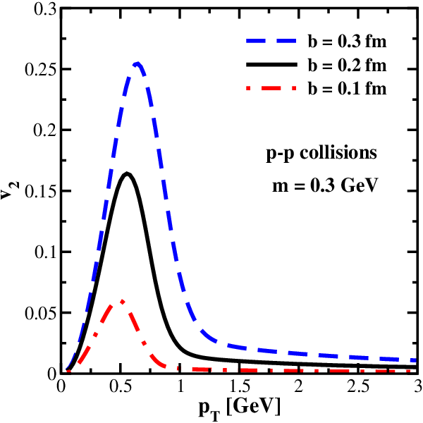
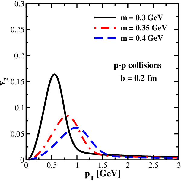
In Fig. 6 we show the azimuthal asymmetry computed according to Eqs. (III.3), (33) and (40) for different choices of the central saturation scale . These plots illustrate the scaling of the peak position with : when we plot as a function of , the peak position is quasi independent of and rather close to 1/2. This scaling property indicates the importance of the saturation physics. A larger saturation scale shifts the unintegrated gluon distribution (the integrand of ) to higher transverse momenta. In Fig. 7 we show the dependence of the azimuthal asymmetry upon the impact parameter (left panel) and upon the infrared cutoff (right panel). As expected, the strength of is increasing with . Remarkably though, one see that quite large peak values are obtained already for not so large impact parameters, fm, that is, for collisions which are peripheral, but not ultra-peripheral. (Recall that the typical transverse size of the color charge distribution in the target is fm.) It is also interesting to notice that, albeit the height of the peak is rapidly increasing with , its position changes only slightly when going from rather central ( fm) to more peripheral ( fm) values. This observation should be correlated with the fact that, as manifest on Eq. (39), the piece of the amplitude which is responsible for the angular dependence is proportional to the central value of the saturation scale, and not to its local value at the actual impact parameter. As anticipated, the -dependence is quite strong: a slight increase in , from 0.3 GeV to 0.4 GeV, reduces the peak value of by a factor 3.


Turning now to an extended projectile with a Gaussian distribution in impact parameter space, the corresponding is shown in Fig. 8, for various values for and . (We have checked that the -dependence of the results is similar to that observed for a point-like projectile, cf. Fig. 7.) One may expect the strength of the azimuthal asymmetry to be reduced, perhaps even significantly, after averaging over the surface of the projectile, but this is actually not the case: as visible in Fig. 8, the peak value of remains as large as for a point-like projectile. To see such a sizable , however, one needs to go to larger values for the impact parameter , which now refers to the center of the projectile (recall Fig. 1). This is in agreement with the discussion at the end of Sect. III.3, which also suggests that the value of should be correlated to the eccentricity of the interaction region.
To check this conjecture, we have numerically computed and according to Eqs. (43)–(44), with the results shown in Fig. 9 (left panel). These results should be compared to the -dependence of , as exhibited in the right panel of the same figure. These plots confirm that and show a similar trend with : they monotonously increase with — actually, they are both proportional to so long as is small enough, . On the other hand, they show rather different behaviors with . The plots for in the right panel of Fig. 9 are in agreement with those in the left panel of Fig. 8: vanishes as and has a pronounced peak at with GeV. On the other hand, has a rather weak dependence upon : the curves corresponding to different values for the momentum are rather close to each other, and also to the curve representing the integrated eccentricity . This reflects the fact that the quantity is only weakly sensitive to the dipole scattering, since mostly controlled by the geometry.


We now turn to the case of collisions, for which the present formalism is somewhat better justified. The respective is computed by numerically integrating Eq. (57) with the dipole amplitude given by the analytic results in Eqs. (54) and (55). The two plots in Fig. 10, which exhibit as a function of (left panel) and (right panel), for different values of the proton saturation scale , are quite similar to the corresponding plots for collisions, cf. Fig. 6. In particular, the peak position appears to respect the expected scaling with the nuclear saturation momentum : indeed, the maximum occurs at, roughly, , which is larger by a factor (for ) than the respective value observed for collisions. However, in order to reach values for which are comparable to those in collisions, one now needs to go up to much larger values of the impact parameter , there the inhomogeneity in the nuclear distribution is located (cf. the discussion in Sect. III.4). The -dependence of the function is illustrated in the left panel of Fig. 11. This is controlled by the combination , cf. Eq. (53), and the results in Fig. 11 are indeed in agreement with the previous discussion of Fig. 5. Namely, is seen to be sizable and positive for all values fm.
Notice that in the present approximations, the dipole amplitude (hence our estimate for ) for the case of a nuclear target depends upon the two scales and mostly via their product . (This becomes obvious by inspection of Eqs. (54) and (55).) Accordingly, the effect of increasing at fixed , as visible in Fig. 10, can alternatively be associated with increasing for a fixed value . In the right panel of Fig. 11, we show the dependence of in collisions upon the infrared cutoff . Similarly to the case of collisions, one finds that this dependence is rather strong: by decreasing from the ‘confinement’ value GeV to the pion mass GeV, one increases the peak value of by a factor of 3.


In Fig. 12 we illustrate the effect of using an extended proton projectile, with Gaussian distribution in impact parameter. The corresponding formula for is the straightforward generalization of Eq. (42), obtained by replacing and . As visible in Fig. 12, the effect is quite small — at most a change of 20% in the value of at its peak.
The systematics of the above results for can be physically understood as follows. First of all, we found that is small for both very small and very large values of , but has a maximum at some intermediate value . In particular, for , as already obvious by inspection of Eq. (6). These features are easy to understand: the angular orientation cannot play any role when either the momentum , or the dipole size , are too small. Since typically , the second argument explains the rapid decrease of that we observe at high . But the detailed shape of the function — in particular the position, the width, and the height of its maximum — are strongly dependent upon the impact parameter and also upon the values of the 3 parameters , , and .
Specifically, as visible in the left panels in both Fig. 7 and Fig. 11, is negligible for relatively small impact parameters (in particular, it vanishes as ), but it becomes large — in the sense that it reaches a peak value — when the impact parameter is comparable to the typical size for inhomogeneity in the target, that is, fm for a proton and respectively fm for a large nucleus. This is understandable, given that the angular orientation would play no role for a target which is homogeneous in impact-parameter space. We recall that, for the mechanism under consideration, the elliptic flow is driven by the sensitivity of the color-dipole orientation to the variation in the gluonic or nuclear distribution in the transverse plane.
We furthermore found that the peak in moves towards larger values of and becomes broader when increasing , see Fig. 6 and Fig. 10. This is as expected: the larger saturation momentum in the target, the larger is the typical momentum of the produced parton and the wider is its distribution in . Interestingly, for both and collisions we found that the position of the peak in is proportional to . A similar observation was recently made in Ref. [60]. When is plotted as a function of , the peak position is quasi-independent of , albeit its height and shape are still strongly dependent (see the right panels in Fig. 6 and Fig. 10). Specifically, the maximal value at the peak appears to increase when decreasing , i.e. when the target becomes more dilute. This may seem counter-intuitive since, as already stressed, the multiple scattering represents an essential ingredient of the mechanism under consideration (it even changes the sign of as compared to the single-scattering approximation). However, the importance of the dipole orientation depends in a crucial way upon the balance between the dipole size and the size of its impact parameter. The dipole size is fixed by the transverse momentum of the produced quark, , which in turn is determined by the target saturation momentum: . Hence, if one keeps increasing , the dipole size eventually becomes much smaller than and the dipole orientation plays no role anymore. A similar effect is seen when the saturation momentum increases as a consequence of the high-energy evolution [40, 44, 45].
Finally, given the importance of soft, non-perturbative, exchanges for the angular-dependence of the dipole amplitude, is should be no surprise that our results for are rather strongly dependent to the ‘confinement’ scale : the anisotropy is enhanced when decreasing , since the phase-space for soft exchanges is rapidly increasing, see the right panels in Fig. 7 and Fig. 11. For the angular-dependent piece of the dipole amplitude and for a proton target, this dependence has been already exhibited in Fig. 2, whereas for a nuclear target, it is directly visible by inspection of Eq. (55) for .

From the previous considerations in this paper, it should be clear that our current analytic description for the mechanism under consideration is too crude to allow for quantitative predictions, or realistic applications to the phenomenology. This being said, we would like to show via an example that this scenario is not excluded by the current data. Namely, we will show that, by appropriately choosing the values of the impact parameter and of the free parameters of the models, one can give a reasonable description of the -dependence of the elliptic flow extracted from multi-particle azimuthal correlations in p+Pb collisions at the LHC, in a given multiplicity class. This should not be confounded with a genuine fit to the data — it is merely an exploratory comparison. Given the uncertainties inherent in our model, we shall adopt a rather crude strategy for relying the predictions of this model to the phenomenology.
First, we have not attempted to compute the consequences of our mechanism for multi-particle azimuthal correlations; rather, we shall make the simplifying assumption that the final particles are correlated with each other only through the flow correlations with the reaction plane (that is, we neglect possible ‘non-flow correlations’). Under this assumption, we can write , and similarly , where and are the second-order two-particle and respectively four-particle cumulants, as defined e.g. in [83, 49], and is the usual elliptic flow coefficient, as discussed throughout this paper. More precisely, our present estimates for refer to a fixed impact parameter , that is, we have a prediction for the function , whereas the data for p+Pb (and also p+p) collisions are rather classified according to the particle multiplicity (the number of reconstructed tracks) in the final state. Due to the large multiplicity fluctuations, the correlation between the multiplicity classes and the cuts in impact parameter is rather loose and not well under control (see e.g. the discussion in [84]). To cope with that and by lack of any better alternative, we shall simply select a value of for which the predictions of our model appear to reasonably agree with the data in a given high-multiplicity class. We shall similarly proceed with the free parameters of our model, which in the case of collisions are the dimensionless product and the infrared cutoff . It is understood that the values for , and which will emerge from this procedure must also reflect the influence of other uncertainties or simplifications inherent in our present approach, like the omission of gluons. (Gluon production within the present set-up should give rise to a similar -dependence in , but only modify its overall magnitude.)
Finally, to have a better comparison with the -dependence of the data, which refer to hadrons, one must take into the account the effect of the quark (or gluon) fragmentation into hadrons. This too will be implemented in a rather heuristic way, by assuming that where is the average value of the splitting fraction and will be treated as a free parameter.
In Fig. 13, we compare our results for in peripheral collisions (with ) with the experimental data from the CMS experiment for the second-order elliptic harmonic in p-Pb collisions, as extracted from a four-particle cumulant analysis in events where the number of reconstructed tracks lies in the range [3]. The two theoretical curves are obtained by using an extended projectile (so the impact parameter refers to the center of this projectile, as in Fig. 12), together with the following values for the free parameters: fm, , GeV2, GeV, and two values for : 0.6 and respectively 0.7. Notice that this value GeV2 is in the ballpark of the theoretical expectations for the proton saturation momentum at the LHC energies. It is quite remarkable that, in spite of the many simplifications and the crude assumptions, our mechanism appears to be able to produce the correct -dependence of and also its correct size, with reasonable values for the free parameters.
V Conclusions and perspectives
In this paper, we have analyzed a less explored, albeit not totally new, mechanism for generating azimuthal asymmetries in particle production in ‘dilute-dense’ collisions: the dependence of the cross-section for single-inclusive particle production upon the azimuthal orientation of the momentum of the produced particle w.r.t. its impact parameter. As compared to previous related studies in the literature [56, 57, 58, 32, 59, 60], we have considered a different model for the gluon distribution in the dense target — an extension of the McLerran-Venugopalan (MV) model — which combines the proper pQCD tail at high transverse momenta with a Gaussian profile (inspired by fits to the HERA data) for the distribution of the color charges in the impact-parameter space and a ‘gluon mass’ which mimics confinement. A realistic, or at least physically motivated, treatment of the non-perturbative aspects related to the transverse inhomogeneity and to confinement is indeed essential, since, as demonstrated by our analysis, these aspects do actually control the azimuthal asymmetries produced by this mechanism.
Within this set-up, we have given a systematic, semi-analytic, study of the angular dependence of the dipole scattering amplitude and we have used the result to compute the elliptic flow coefficient , separately for proton-proton and proton-nucleus collisions (the main difference being the inclusion of lumpiness effects in the case of a nuclear target). We thus found that, as a function of the impact parameter, is rather strongly peaked near the edge of the target, where the transverse inhomogeneity is more pronounced. Hence the present mechanism will significantly contribute to azimuthal asymmetries only via peripheral collisions. Furthermore, as a function of the transverse momentum of the produced particle, shows a maximum at some intermediate, semi-hard, value which is proportional to the target saturation momentum at . This maximum broadens and lowers with increasing the saturation momentum. The overall -dependence is quite similar to that observed in the phenomenology of p+Pb collisions at the LHC. In fact, a semi-quantitative agreement with the data can be obtained with reasonable choices for the model parameters, but this agreement should be taken with a grain of salt, because our model is quite crude and additional approximations are performed when comparing with the data.
To convincingly demonstrate this mechanism, further studies are necessary. First, one would like to understand its evolution with increasing energy. To that aim, one should solve the Balitsky-Kovchegov (BK) equation [85, 86] with initial conditions at low energy provided by our present model. In the respective solutions, one must keep trace of the impact-parameter dependence (including the angular dependence) of the dipole amplitude and one must enforce confinement within the soft gluon emission kernel, preferably by using the same infrared regulator (‘gluon mass’) as in the initial condition. Similar solutions have been already considered in [87, 69, 70].
Furthermore, since the orientation of the reaction plane cannot be experimentally measured, one must compute the imprint of the azimuthal asymmetries generated by the present mechanism on multi-particle correlations. For instance, one can study the simultaneous production of 2 quarks in collisions. The calculation can be simplified by assuming that the two quarks (originally collinear with the projectile) scatter independently of each other and by taking the multicolor limit . (We recall that the multi-particle correlations generated by the present mechanism survive in the large- limit.) As anticipated in the Introduction, we expect the multi-particle correlations to be important only for sufficiently peripheral collisions and to lead to flow — a collective motion of particles which are produced independently from each other, but which are all correlated with the reaction plane defined by their average impact parameter. Note that even for independent partons in the projectile at large , the double-patron-scattering (DPS) Hanbury Brown and Twiss (HBT) correlations may lead to anisotropy [88]. This effect is not accounted for in the present mechanism.
Given the prominence of the peripheral physics for the physical problem at hand, we furthermore expect that the fluctuations in the shape of the colliding hadrons should play an important role: they should amplify the inhomogeneity in impact parameter space and thus enhance the azimuthal asymmetries. The importance of such fluctuations is supported by a recent analysis of the HERA data for incoherent exclusive diffractive vector meson production in deep inelastic scattering [89]. It would be therefore interesting to redo our present analysis of the angular dependence of the dipole scattering for the case where the (projectile and/or target) proton has strong shape fluctuations, say as described by the models used in [89] and which are constrained by the HERA data.
Acknowledgements.
We would like to thank Y. Hagiwara, Y. Hatta, B.-W. Xiao, and F. Yuan for sharing with us a preliminary version of their recent work [60] and for related discussions. We are grateful to T. Lappi, J.-Y. Ollitrault and L. McLerran for comments on the manuscript. This research was supported in part by ECOS-Conicyt C14E01. The work of E.I. was supported in part by the Agence Nationale de la Recherche project ANR-16-CE31-0019-01. The work of A.R. was supported in part by Fondecyt grant 1150135, Anillo ACT1406 and Conicyt PIA/Basal FB0821.Appendix A Computing the dipole amplitude in the two-gluon exchange approximation
In this Appendix, we present details on the calculation leading to Eqs. (III.3) and (33) for the dipole scattering amplitude in the two-gluon exchange approximation. The starting point is Eq. (29) for , which, we recall, has been obtained from the general MV-model formula (20) by expanding to second order in .
Specifically, let and denote the angles between and and, respectively, between and . Then we can rewrite Eq. (29) as
| (58) | |||||
We first perform the integral over the angle using the identity in Eq. (5), to obtain
| (59) |
The ensuing integrals over can be now performed by using the following identities
| (60) |
with and . We thus confirm the general structure in Eq. (31) and at the same time obtain more explicit expressions for the two functions and , as double radial integrals to be numerically computed. Specifically, we find
| (61) |
together with Eq. (33) for . It is easy to check that the double integral yielding is well defined as is stands, so its numerical evaluation poses no special problem. On the other hand, the integral over giving has a logarithmic ultraviolet divergence and needs to be cut off at , as already explained. The precise implementation of this UV cutoff introduces some ambiguity, that we shall fix by replacing Eq. (61) with Eq. (III.3), as discussed in the main text.
As also explained in Sect. III.2, the limit of is well defined, because of the explicit transverse inhomogeneity in the target. We have already studied this limit for the piece which controls the angular dependence, cf. Eq. (39). In what follows we shall perform the corresponding study for the other piece . To that aim, it is more convenient to use Eq. (61), in which we set and simply cut the integral over in the ultraviolet at . Using Eq. (37), we find
| (62) | |||||
This is strictly true for , meaning (recall that the integral over is restricted to by the transverse inhomogeneity in the target). At this point, it is convenient to separate the logarithm as , where the first piece in the r.h.s. is the ‘large logarithm’ (since typically ), whereas the argument of the second logarithm is of order one. One then easily finds
| (63) | |||||
where in the second line we kept only the power-law tail at large , as developed by the integral over from the first line. (This power law tail can be easily obtained by letting inside the integrand, as appropriate for large .) Notice that for very large impact parameters , the first term proportional to the local saturation momentum is exponentially suppressed and the scattering amplitude (which is small anyway) is controlled by the power-law tail. However, this is not the situation that we have considered throughout this work; indeed, we have looked at impact parameters , where the scattering amplitude is dominated by the first term .
Appendix B More details on the case of a lumpy nuclear target
In this Appendix, we shall present more details on the derivation of Eqs. (54) and (55) for the dipole scattering off a lumpy nucleus in the two-gluon exchange approximation. Namely, we would like to compute the integral over in Eq. (50) with the nuclear thickness function given by the second-order expansion in Eq. (51). To that aim, it is useful to introduce the following Fourier transform
| (64) |
To the order of interest, is given by Eq. (29), which immediately implies
| (65) |
The interesting integrals over can be related to the behavior of near . We first have
| (66) |
We have also used here together with the renormalization prescription in Eq. (34) and . Not surprisingly, the integral over has generated a result proportional to the proton area .
For the terms quadratic in , one similarly finds
| (67) | |||||
where in going from the second to the third line we have used the fact that, under the integral over , one can replace
| (68) |
By combining the above equations (66) and (67) with the expansion in Eq. (51), one immediately finds the results exhibited in Eqs. (54) and (55).
References
- [1] V. Khachatryan et al. (CMS), JHEP 09, 091 (2010), eprint 1009.4122.
- [2] S. Chatrchyan et al. (CMS), Phys.Lett. B718, 795 (2013a), eprint 1210.5482.
- [3] S. Chatrchyan et al. (CMS), Phys. Lett. B724, 213 (2013b), eprint 1305.0609.
- [4] B. Abelev et al. (ALICE), Phys.Lett. B719, 29 (2013a), eprint 1212.2001.
- [5] B. B. Abelev et al. (ALICE), Phys. Lett. B726, 164 (2013b), eprint 1307.3237.
- [6] B. B. Abelev et al. (ALICE), Phys. Rev. C90, 054901 (2014), eprint 1406.2474.
- [7] G. Aad et al. (ATLAS Collaboration), Phys.Rev.Lett. 110, 182302 (2013a), eprint 1212.5198.
- [8] G. Aad et al. (ATLAS Collaboration), Phys.Lett. B725, 60 (2013b), eprint 1303.2084.
- [9] G. Aad et al. (ATLAS), Phys. Rev. C90, 044906 (2014), eprint 1409.1792.
- [10] A. Adare et al. (PHENIX), Phys. Rev. Lett. 111, 212301 (2013), eprint 1303.1794.
- [11] A. Adare et al. (PHENIX), Phys. Rev. Lett. 114, 192301 (2015), eprint 1404.7461.
- [12] L. Adamczyk et al. (STAR), Phys. Lett. B743, 333 (2015a), eprint 1412.8437.
- [13] L. Adamczyk et al. (STAR), Phys. Lett. B747, 265 (2015b), eprint 1502.07652.
- [14] D. d’Enterria, G. K. Eyyubova, V. L. Korotkikh, I. P. Lokhtin, S. V. Petrushanko, L. I. Sarycheva, and A. M. Snigirev, Eur. Phys. J. C66, 173 (2010), eprint 0910.3029.
- [15] P. Bozek, Eur. Phys. J. C71, 1530 (2011), eprint 1010.0405.
- [16] P. Bozek and W. Broniowski, Phys. Lett. B718, 1557 (2013a), eprint 1211.0845.
- [17] P. Bozek and W. Broniowski, Phys. Rev. C88, 014903 (2013b), eprint 1304.3044.
- [18] P. Bozek, W. Broniowski, and G. Torrieri, Phys. Rev. Lett. 111, 172303 (2013), eprint 1307.5060.
- [19] G.-Y. Qin and B. M�ller, Phys. Rev. C89, 044902 (2014), eprint 1306.3439.
- [20] K. Werner, M. Bleicher, B. Guiot, I. Karpenko, and T. Pierog, Phys. Rev. Lett. 112, 232301 (2014), eprint 1307.4379.
- [21] A. Bzdak and G.-L. Ma, Phys. Rev. Lett. 113, 252301 (2014), eprint 1406.2804.
- [22] R. D. Weller and P. Romatschke (2017), eprint 1701.07145.
- [23] Y. V. Kovchegov, E. Levin, and L. D. McLerran, Phys. Rev. C63, 024903 (2001), eprint hep-ph/9912367.
- [24] D. Teaney and R. Venugopalan, Phys. Lett. B539, 53 (2002), eprint hep-ph/0203208.
- [25] Y. V. Kovchegov and K. L. Tuchin, Nucl. Phys. A708, 413 (2002), eprint hep-ph/0203213.
- [26] A. Dumitru, F. Gelis, L. McLerran, and R. Venugopalan, Nucl.Phys. A810, 91 (2008), eprint 0804.3858.
- [27] S. Gavin, L. McLerran, and G. Moschelli, Phys. Rev. C79, 051902 (2009), eprint 0806.4718.
- [28] E. Avsar, C. Flensburg, Y. Hatta, J.-Y. Ollitrault, and T. Ueda, Phys. Lett. B702, 394 (2011), eprint 1009.5643.
- [29] A. Dumitru, K. Dusling, F. Gelis, J. Jalilian-Marian, T. Lappi, et al., Phys.Lett. B697, 21 (2011), eprint 1009.5295.
- [30] A. Kovner and M. Lublinsky, Phys. Rev. D83, 034017 (2011a), eprint 1012.3398.
- [31] A. Kovner and M. Lublinsky, Phys.Rev. D84, 094011 (2011b), eprint 1109.0347.
- [32] E. Levin and A. H. Rezaeian, Phys. Rev. D84, 034031 (2011), eprint 1105.3275.
- [33] E. Iancu and D. Triantafyllopoulos, JHEP 1111, 105 (2011), eprint 1109.0302.
- [34] B. Schenke, P. Tribedy, and R. Venugopalan, Phys. Rev. Lett. 108, 252301 (2012a), eprint 1202.6646.
- [35] B. Schenke, P. Tribedy, and R. Venugopalan, Phys. Rev. C86, 034908 (2012b), eprint 1206.6805.
- [36] K. Dusling and R. Venugopalan, Phys. Rev. Lett. 108, 262001 (2012), eprint 1201.2658.
- [37] K. Dusling and R. Venugopalan, Phys. Rev. D87, 094034 (2013), eprint 1302.7018.
- [38] K. Dusling, P. Tribedy, and R. Venugopalan, Phys. Rev. D93, 014034 (2016), eprint 1509.04410.
- [39] Y. V. Kovchegov and D. E. Wertepny, Nucl. Phys. A925, 254 (2014), eprint 1310.6701.
- [40] A. Kovner and M. Lublinsky, Int. J. Mod. Phys. E22, 1330001 (2013), eprint 1211.1928.
- [41] A. Kovner and A. H. Rezaeian, Phys. Rev. D90, 014031 (2014), eprint 1404.5632.
- [42] A. Kovner and A. H. Rezaeian, Phys. Rev. D92, 074045 (2015), eprint 1508.02412.
- [43] B. Schenke, S. Schlichting, and R. Venugopalan, Phys. Lett. B747, 76 (2015), eprint 1502.01331.
- [44] T. Lappi, Phys. Lett. B744, 315 (2015), eprint 1501.05505.
- [45] T. Lappi, B. Schenke, S. Schlichting, and R. Venugopalan, JHEP 01, 061 (2016), eprint 1509.03499.
- [46] A. H. Rezaeian, Phys. Rev. D93, 094030 (2016), eprint 1603.07354.
- [47] B. Schenke and S. Schlichting, Phys. Rev. C94, 044907 (2016), eprint 1605.07158.
- [48] B. Schenke, S. Schlichting, P. Tribedy, and R. Venugopalan, Phys. Rev. Lett. 117, 162301 (2016), eprint 1607.02496.
- [49] R. Snellings, New J. Phys. 13, 055008 (2011), eprint 1102.3010.
- [50] B. Alver and G. Roland, Phys. Rev. C81, 054905 (2010), [Erratum: Phys. Rev.C82,039903(2010)], eprint 1003.0194.
- [51] E. Iancu and R. Venugopalan (2003), eprint hep-ph/0303204.
- [52] F. Gelis, E. Iancu, J. Jalilian-Marian, and R. Venugopalan, Ann.Rev.Nucl.Part.Sci. 60, 463 (2010), eprint 1002.0333.
- [53] A. Dumitru and A. V. Giannini, Nucl. Phys. A933, 212 (2015), eprint 1406.5781.
- [54] A. Dumitru and V. Skokov, Phys. Rev. D91, 074006 (2015), eprint 1411.6630.
- [55] A. Dumitru, L. McLerran, and V. Skokov, Phys. Lett. B743, 134 (2015), eprint 1410.4844.
- [56] B. Z. Kopeliovich, H. J. Pirner, A. H. Rezaeian, and I. Schmidt, Phys. Rev. D77, 034011 (2008a), eprint 0711.3010.
- [57] B. Z. Kopeliovich, A. H. Rezaeian, and I. Schmidt, Nucl. Phys. A807, 61 (2008b), eprint 0712.2829.
- [58] B. Z. Kopeliovich, A. H. Rezaeian, and I. Schmidt, Phys. Rev. D78, 114009 (2008c), eprint 0809.4327.
- [59] J. Zhou, Phys. Rev. D94, 114017 (2016), eprint 1611.02397.
- [60] Y. Hagiwara, Y. Hatta, B.-W. Xiao, and F. Yuan (2017), eprint 1701.04254.
- [61] L. D. McLerran and R. Venugopalan, Phys. Rev. D49, 3352 (1994), eprint hep-ph/9311205.
- [62] H. Kowalski and D. Teaney, Phys.Rev. D68, 114005 (2003), eprint hep-ph/0304189.
- [63] H. Kowalski, T. Lappi, C. Marquet, and R. Venugopalan, Phys.Rev. C78, 045201 (2008), eprint 0805.4071.
- [64] A. H. Rezaeian, M. Siddikov, M. Van de Klundert, and R. Venugopalan, Phys.Rev. D87, 034002 (2013), eprint 1212.2974.
- [65] E. Iancu, K. Itakura, and S. Munier, Phys. Lett. B590, 199 (2004), eprint hep-ph/0310338.
- [66] H. Kowalski, L. Motyka, and G. Watt, Phys.Rev. D74, 074016 (2006), eprint hep-ph/0606272.
- [67] A. H. Rezaeian and I. Schmidt, Phys.Rev. D88, 074016 (2013), eprint 1307.0825.
- [68] S. Munier, A. M. Stasto, and A. H. Mueller, Nucl. Phys. B603, 427 (2001), eprint hep-ph/0102291.
- [69] J. Berger and A. M. Stasto, Phys.Rev. D84, 094022 (2011), eprint 1106.5740.
- [70] J. Berger and A. M. Stasto, JHEP 01, 001 (2013), eprint 1205.2037.
- [71] N. Armesto and A. H. Rezaeian, Phys. Rev. D90, 054003 (2014), eprint 1402.4831.
- [72] Y. V. Kovchegov, L. Szymanowski, and S. Wallon, Phys. Lett. B586, 267 (2004), eprint hep-ph/0309281.
- [73] Y. Hatta, E. Iancu, K. Itakura, and L. McLerran, Nucl. Phys. A760, 172 (2005), eprint hep-ph/0501171.
- [74] J. L. Albacete, N. Armesto, J. G. Milhano, P. Quiroga-Arias, and C. A. Salgado, Eur.Phys.J. C71, 1705 (2011), eprint 1012.4408.
- [75] E. Iancu, J. D. Madrigal, A. H. Mueller, G. Soyez, and D. N. Triantafyllopoulos, Phys. Lett. B750, 643 (2015a), eprint 1507.03651.
- [76] J. L. Albacete, Nucl. Phys. A957, 71 (2017), eprint 1507.07120.
- [77] J. Jalilian-Marian and A. H. Rezaeian, Phys.Rev. D85, 014017 (2012), eprint 1110.2810.
- [78] J. L. Albacete, A. Dumitru, H. Fujii, and Y. Nara, Nucl.Phys. A897, 1 (2013), eprint 1209.2001.
- [79] A. H. Rezaeian, Phys.Lett. B718, 1058 (2013), eprint 1210.2385.
- [80] Y. Hatta, E. Iancu, C. Marquet, G. Soyez, and D. Triantafyllopoulos, Nucl.Phys. A773, 95 (2006), eprint hep-ph/0601150.
- [81] G. Beuf, Phys.Rev. D89, 074039 (2014), eprint 1401.0313.
- [82] E. Iancu, J. Madrigal, A. Mueller, G. Soyez, and D. Triantafyllopoulos, Phys.Lett. B744, 293 (2015b), eprint 1502.05642.
- [83] N. Borghini, P. M. Dinh, and J.-Y. Ollitrault, Phys. Rev. C63, 054906 (2001), eprint nucl-th/0007063.
- [84] J. Adam et al. (ALICE), Phys. Rev. C91, 064905 (2015), eprint 1412.6828.
- [85] I. Balitsky, Nucl. Phys. B463, 99 (1996), eprint hep-ph/9509348.
- [86] Y. V. Kovchegov, Phys. Rev. D60, 034008 (1999), eprint hep-ph/9901281.
- [87] L. Motyka and A. M. Stasto, Phys.Rev. D79, 085016 (2009), eprint 0901.4949.
- [88] A. Kovner and A. H. Rezaeian (2017), eprint 1701.00494.
- [89] H. M�ntysaari and B. Schenke, Phys. Rev. D94, 034042 (2016), eprint 1607.01711.