A Study on the Impact of Locality in the Decoding of Binary Cyclic CodesThanks: ^a Department of Electrical Communication Engineering, Indian Institute of Science, Bangalore, India, Email: nikhilkrishnan.m@gmail.com. Research supported through Visvesvaraya PhD Scheme for Electronics & IT awarded by Department of Electronics and Information Technology, Govt. of India. ^b Department of Electrical Communication Engineering, Indian Institute of Science, Bangalore, India, Email: bhagya.puranik@gmail.com ^c Department of Electrical Communication Engineering, Indian Institute of Science, Bangalore, India, Email: pvk1729@gmail.com. P. V. Kumar is also an Adjunct Research Professor at the University of Southern California. His research is supported in part by NSF under Grant No. 1421848 and in part by the joint UGC-ISF research program. ^d Department of EE-Systems, Tel Aviv University, Tel Aviv, Israel, Email: zactamo@gmail.com. Research is supported by ISF grant no. 1030/15 and the NSF-BSF grant no. 2015814. ^e Dept. of ECE and ISR, University of Maryland, College Park, USA, and Inst. Inform. Trans. Probl. (IITP), Russian Academy of Sciences, Moscow, Russia, Email: abarg@umd.edu. Research is supported in part by NSF grants CCF1422955 and CCF1618603.

All the codes discussed in this paper are assumed to be linear of length $n$ and dimension $k$ over a field $\mathbb{F}_{q}$ unless specified otherwise, and we write their parameters as $[n,k].$ Let $[l]\triangleq\{1,2,\ldots,l\}$ and $[0,l]\triangleq\{0,1,\ldots,l\}$.

The codes studied in this paper belong to the class of LRC codes [7]. We begin with a definition, limiting ourselves to the linear case.

The subset ${\mathcal{I}}_{i}$ is called the recovery set of the coordinate $i$. It is clear that every coordinate $j\in{\mathcal{I}}_{i}\cup\{i\}$ can be found from the remaining coordinates in this set, so we call the set ${\mathcal{I}}_{i}\cup\{i\}$ a repair group. Most constructions of LRC codes in the literature, including those in [18, 17, 20] and the codes considered in this paper, have the property of disjoint repair groups (for brevity we call them codes with disjoint locality).

The following generalization of this definition was suggested in [13].

Further, $\mathcal{C}$ is said to possess $(r,\delta)$-information locality if there exists an information set $\mathcal{I}\subseteq[0,n-1]$ such that $\mathbf{G}_{\mathcal{I}}$ ($\mathbf{G}$ punctured to the coordinates in $\mathcal{I}$) has rank $k$ and all $i\in\mathcal{I}$ have $(r,\delta)$-code-symbol locality. Similarly, if every code-symbol $c_{i}$, $i\in[0,n-1]$ has $(r,\delta)$-code-symbol locality, the code is said to have $(r,\delta)$-all-symbol locality. Codes with locality $r$ defined above [7] form a particular case of this definition for $\delta=2$. For any code $r\leq k$, because (unless the distance of $\mathcal{C}$ is $1$), $\mathbf{G}$ contains $k$ linearly independent columns that do not include any chosen coordinate $i$.

We define the support of a set of codewords $\mathcal{D}$ as $\text{supp}({\mathcal{D}})\triangleq\cup_{\underline{c}\in{\mathcal{D}}}\text{supp}(\underline{c}).$

This definition can be extended to more than two levels of local code hierarchy.

Consider an $[n,k]$ cyclic code $\mathcal{C}$ over a field $\mathbb{F}_{q}$ such that $(n,q)=1$ and $n|(q^{m}-1)$, where $m$ is the multiplicative order of $q$ modulo $n$. Let $\alpha\in\mathbb{F}_{q^{m}}$ be a primitive $n^{\text{th}}$ root of unity. Given a codeword $\underline{c}=(c_{0},c_{1},\dots,c_{n-1}),$ let $c(x)=\sum_{i=0}^{n-1}c_{i}x^{i}.$ Let $\alpha^{i_{1}},\alpha^{i_{2}},\dots$ be the set of common zeros of these polynomials in the set of $n^{\text{th}}$ roots of unity. By abuse of terminology, we call the set $\mathcal{S}(\mathcal{C})\triangleq\{i_{1},i_{2},\dots\}$ the set of the zeros of the code $\mathcal{C}.$ Recall that if $i$ is a zero of $\mathcal{C}$, then so is $qi\text{\,mod\,}n$, and the set of distinct elements among $\{(q^{j}i)\text{\,mod\,}n,j=1,2,\dots\}$ is called the cyclotomic coset of $i.$ We note that a cyclic code is fully described by specifying only the representatives of cyclotomic cosets.

Let $\mathcal{I}\subseteq[0,n-1]$ be a subset of code coordinates. The codes having length $|\mathcal{I}|$ obtained by shortening and puncturing $\mathcal{C}$ to $\mathcal{I}$ are denoted by $\mathcal{C}^{\mathcal{I}}$ and $\mathcal{C}_{\mathcal{I}}$, respectively. Let $n_{1}|n$ and $\nu\triangleq\frac{n}{n_{1}}$. We define the following set: $\mathcal{I}_{i}\triangleq\{i,i+\nu,i+2\nu,\ldots,i+n-\nu\}$, where $0\leq i\leq\nu-1$, which may be regarded as being obtained by shifting and then decimating the set $[0,n-1]$. We will call each such set a length-$n_{1}$ support set. It can be verified that $\mathcal{C}_{\mathcal{I}_{i}}$’s (and similarly, $\mathcal{C}^{\mathcal{I}_{i}}$’s) are all identical for $0\leq i\leq\nu-1$ and are moreover cyclic codes of length $n_{1}$. We refer to these codes as length-$n_{1}$ punctured (and similarly, shortened) codes of $\mathcal{C}$. The zeros of these codes will be assumed to be computed with respect to the exponents of $\beta=\alpha^{\nu}$. We cite below a result from [19] which relates the zeros $\mathcal{S}(\mathcal{C}^{\mathcal{I}_{i}})$ of the shortened code to $\mathcal{S}(\mathcal{C})$:

We derive the following analogous lemma for punctured codes.

The proof of this lemma is given in Appendix -B. We call the set ${\mathcal{T}}_{a}^{(n_{1})}\triangleq\{a,a+n_{1},\ldots,a+(\nu-1)n_{1}\}$, where $a\in[0,n_{1}-1]$, a locality train corresponding to $n_{1}.$

A sufficient condition for a cyclic code to have $r$-all-symbol locality in terms of its zeros was proved in [17] and is stated in the theorem that follows. We use Lemma-II.2 to give an alternate proof of this theorem.

The above result can be extended to the case of $(r,\delta)$-locality for $\delta>2$, and is given below. This theorem also generalizes a similar result that appears in [20].

We invoke Lemma-II.2 to show the existence of hierarchical locality in the example below.

We summarize the OSD algorithm due to Fossorier et al. [4] as follows. We consider the channel with additive white Gaussian noise (AWGN), where the transmitted vector is ${\underline{x}}=(x_{0}\ x_{1}\ \ldots\ x_{n-1})$, with $x_{i}\in\{+1,-1\}$. The received vector is ${\underline{y}}={\underline{x}}+{\underline{n}}$, with $n_{i}\sim\mathcal{N}(0,\frac{N_{0}}{2}),$ and $N_{0}$ is the power spectral density of the noise. Under the OSD algorithm, the received vector is first ordered in decreasing order of the $|y_{i}|$’s, which are regarded as reliability values. We call the first $k$ bits in this order which are linearly independent as Most Reliable Independent (MRI) symbols. We clip their values to the nearest value of $\{1,-1\}$ and regard them as $k$ information bits of the codeword. The corresponding codeword in $\mathcal{C}$, is selected as the order-$0$ OSD algorithm decoded codeword. This may be followed by an order-$l$ reprocessing stage, where, for $0\leq i\leq l$, all possibilities of $i$ bits from the $k$ MRI bits will be flipped to obtain $M=\sum_{i=0}^{l}{k\choose i}$ information sets. The $M$ information sets are mapped to their respective codewords and the codeword with least Euclidean distance from $\underline{y}$ will be declared as the order-$l$ OSD output.

In this section, we primarily consider binary linear codes having either (a) disjoint or (b) hierarchical locality. In the case of disjoint locality, the code is assumed to have $r$-all-symbol-locality, with disjoint supports for local (single parity check) codes. For codes with $h$-level hierarchical locality (say, $h=2$) local codes within each level are assumed to have disjoint supports. Furthermore, the base code parity checks here are assumed to include single-parity checks.

In the locality-aware OSD algorithm, we first consider a supercode of $\mathcal{C}$ denoted by $\mathcal{C}_{\text{loc}}$, whose dual code is precisely the space spanned by the local parity checks on $\mathcal{C}$. The $\mathcal{C}_{\text{loc}}$ is a concatenation (direct sum) of single parity-check codes (similarly, middle codes) for the disjoint (similarly, hierarchical) locality scenario. We carry out ML decoding (which we call quick-look ML decoding, Q-MLD) on the received vector, $\underline{y}$ with the underlying code assumed to be $\mathcal{C}_{\text{loc}}$. The disjoint supports of the local codes permit the local codes to be ML-decoded independently.

In the following, we present simulation results which suggest that locality amongst code symbols can be effectively used to obtain significant gains in SNR with negligible complexity overhead in the BP$+$OS stage. Note that these performance gains are in addition to the reductions in average complexity and delays obtained through the use of Q-MLD. We reiterate that the BP$+$OS scheme that we use is non-iterative and non-adaptive in nature, making it easier to implement, and yet it gives significant performance gains (see [11], [12] for a discussion of adaptive and iterative decoding techniques).

Without loss of generality, we assume transmission of $\underline{1}$ (the all-zero codeword) in the simulations. Fig. 2 presents results relating to two codes; (i) $\mathcal{C}$: the $[255,206]$ BCH code having defining zeros at $\{0,1,3,5,7,9,11\}$ and their $2$-cyclotomic cosets (ii) $\mathcal{B}$: a $[255,192]$ code with locality, $r=16$, obtained from $\mathcal{C}$ using Theorem II.3. The code $\mathcal{B}$ has defining zeros at $\{0,1,3,5,7,9,11,17,51,85,119\}$ and their $2$-cyclotomic cosets. To bring out the impact of introducing locality and taking advantage of it, conventional OSD of order-$0$, $1,$ and $2$ is carried out for both codes and in addition, locality-aware OSD with order-$0$, $1$ and $2$ is carried out for $\mathcal{B}$.

In Fig. 3, we consider the $[255,175]$ majority logic decodable code [5, p.290]. This code has a doubly transitive automorphism group and inherently possesses availability, so we obtain $t=16$ with $r=15$. We perform majority logic codeword decoding, conventional OS of order-$0$, $1$ or $2$. In the locality-aware OSD scheme, likelihoods will be obtained for each symbol, based on $t$ orthogonal parity checks, followed by OSD of order-$0$, $1$ and $2$. Here, we observe that BP+order-$0$ OSD outperforms even conventional order-$2$ OSD in the higher SNR range. For both the simulations, similar trends have been observed with respect to Bit-Error-Rate (BER) performance as well, in the same SNR range. For codes having overlapping local parity checks, preliminary experiments are inconclusive and call for further study.

Given an $[n,k]$ cyclic code $\mathcal{C}$ over $\mathbb{F}_{q}$, it is possible to employ locality to construct a subcode $\mathcal{C}_{\text{new}}\subset\mathcal{C}$ with low trellis complexity. Apart from the obvious dependency of state complexity on the dimension of the punctured code dimensions (viz. (3)), the approach of this section is further motivated by empirical analyses suggesting locality to be a ubiquitous feature in cyclic codes of composite length that have low trellis complexity, with respect to the chain-based orderings we consider. For instance, we considered (via a computer search) all binary cyclic codes of length $n=63$ having low trellis complexity (edge count $\leq 50000$, after fixing the chain to be ${\tau}=\{7,21\}$). Further, we restricted the search to moderate code-rates, $0.2\leq\frac{k}{n}\leq 0.8$. This was because, at very high and very low rates, complexity is bound to be low due to (4). Interestingly, the computer search revealed that all the codes being considered have $r$-all-symbol locality, with $r\leq 19$ (the codes of dimension $k\leq 19$ trivially satisfy this condition), and on an average, the codes had a locality of $10$.

Let $n_{j}|n$. From Lemma-II.2, if the set of zeros of the code $\mathcal{C}$ contains a locality train $\mathcal{T}_{b}^{(n_{j})}=\{b,b+n_{j},b+2n_{j},\ldots,b+n-n_{j}\}$ for some $b\in[0,n_{j}-1],$ then $\mathcal{C}$ has the locality property, with length-$n_{j}$ punctured codes as local codes. Our idea in the remainder of this section is to show that adding locality trains to the set of zeros of the code can be used to reduce the state complexity of resulting subcode. Let $b\in[0,n_{j}-1]$ and let $\mathbb{C}_{b}^{n_{j}}$ be the $q$-cyclotomic coset modulo $n_{j}$ that contains $b.$ Adding $\mathcal{T}_{b}^{(n_{j})}$ to ${\mathcal{S}}(\mathcal{C})$ amounts to taking the subcode ${\mathcal{C}}_{\text{new}}\subset\mathcal{C}$ whose set of zeros is

In the following theorem we quantify our idea of reducing complexity by appending locality trains to the zeros of the code.

Next we derive a bound on the state complexity of cyclic codes. We begin with explaining the idea. Let $\mathcal{C}$ be a cyclic code of composite length (with or without locality). We estimate the state complexity of the permuted code (suppressing the difference between the two versions of the code before and after the permutation). Suppose that the coordinates of the code ${\mathcal{C}}$ are permuted with respect to some chain $\tau=\{x_{1},\dots,x_{L}\}$. It is possible to bound above the state complexity $s_{i}$ relying on its set of zeros $\mathcal{S}(\mathcal{C}).$ Indeed, consider the sections of the trellis at the indices in the set $\tau.$ The corresponding values of the state complexity are governed by the dimensions of the respective past and future codes. From Lemmas II.1 and -II.2, the dimensions of the past codes $\{p^{x_{1}},p^{x_{2}},\ldots,p^{x_{L}}\}$ and $\{p_{x_{1}},p_{x_{2}},\ldots,p_{x_{L}}\}$ can be obtained. Past punctured code dimensions can be expressed in terms of future shortened code dimensions using the rank-nullity theorem, namely

Furthermore, $f_{n-x}=p_{x}$ and $f^{n-x}=p^{x}$, for $x\in\tau$. This follows because the last $x$ coordinates form a length-$x$ support set. Hence the code obtained by puncturing (and similarly, shortening) to the last $x$ coordinates is permutation-equivalent to length-$x$ punctured (resp., shortened) codes of $\mathcal{C}$. Therefore, we can also find the dimensions of the shortened codes $\{p^{n-x_{1}},p^{n-x_{2}},\ldots,p^{n-x_{L}}\}$.

It is straightforward to see that $\{p^{i}:i\in[0,n]\}$ is a non-decreasing sequence bounded above by $k$, and the maximum value of the increase within the $x$-support set is $p^{x}$. Also, $p^{0}\triangleq 0$ and $p^{i+1}-p^{i}\in\{0,1\}$. This enables us to construct a sequence $\{\phi_{i}\}_{i=0}^{n}$ which forms an upper bound for $\{p^{i}\}_{i=0}^{n}$. We begin with defining $\phi_{i}$ for the known instances of $i$:

To fill in the gaps in the sequence, $\{\phi_{i}\}$ we use the constraints on $\{p^{i}\}$ mentioned above. Namely, starting with $i=0$, we either put $\phi_{i+1}=\phi_{i}$ or $\phi_{i+1}=\phi_{i}+1,$ as appropriate. Clearly we have

(the second inequality implied by symmetry). Now let $\mu_{i}=\phi_{i}+\phi_{n-i}-k$ and observe from (3) that $s_{i}\leq\mu_{i}.$

Similar relations can be obtained for the dual code using the well-known relation between $\mathcal{S}(\mathcal{C})$ and $\mathcal{S}(\mathcal{C}^{\perp})$ ($\beta\in\mathcal{S}(\mathcal{C})$ iff $\beta^{-1}\not\in\mathcal{S}(\mathcal{C}^{\perp})$). Using this together with the fact that the state complexity of $\mathcal{C}$ and ${\mathcal{C}}^{\perp}$ is the same [25], we obtain the bound

with $\mu_{i}^{\perp}$ defined accordingly. Note that this bound is tight for $i\in\{0,x_{1},x_{2},\ldots,x_{L},n-x_{L},n-x_{L-1},\ldots,n-x_{1},n\}$.

We can make this argument more explicit by stating an upper bound on the maximum state complexity of the code.

The proof of this theorem is given in Appendix--C.

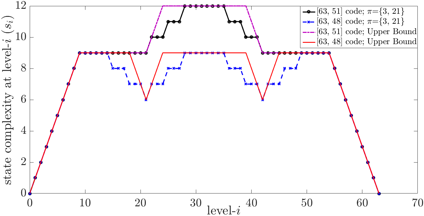
The third term under the $\min\{\}$ can be rewritten as $\sum_{i=0}^{L}h_{i}$, where $h_{i}\triangleq\frac{x_{i+1}}{x_{i}}p^{x_{i}}-p^{x_{i+1}}$, $i>0$, $h_{0}\triangleq x_{1}-p^{x_{1}}$ and $p^{x_{L+1}}=k$. In other words, $h_{i},i>0$ indicates the global parities for the length-$x_{i+1}$ punctured code with respect to smaller length-$x_{i}$ punctured codes. A simple calculation yields that $n-k=h_{0}\frac{n}{x_{1}}+h_{1}\frac{n}{x_{2}}+h_{2}\frac{n}{x_{3}}+\ldots+h_{L}$. This suggests that, for a given $n$ and $k$, the sum $\sum_{i=0}^{L}h_{i}$ can be minimized by making $h_{i}$’s larger for smaller $i$’s (i.e., more locality). The fourth expression accounts for a similar argument about locality of the dual code.

References

- [1] L. R. Bahl, J. Cocke, F. Jelinek, and J. Raviv, “Optimal decoding of linear codes for minimizing symbol error rate (Corresp.),” IEEE Transactions on Information Theory, vol. 20, no. 2, pp. 284–287, 1974.
- [2] J. K. Wolf, “Efficient maximum likelihood decoding of linear block codes using a trellis,” IEEE Transactions on Information Theory, vol. 24, no. 1, pp. 76–80, 1978.
- [3] D. Chase, “A class of algorithms for decoding block codes with channel measurement information,” IEEE Transactions on Information Theory, vol. 18, no. 1, pp. 170–182, 1972.
- [4] M. P. C. Fossorier and S. Lin, “Soft-decision decoding of linear block codes based on ordered statistics,” IEEE Transactions on Information Theory, vol. 41, no. 5, pp. 1379–1396, 1995.
- [5] S. Lin and D. J. Costello, Error Control Coding. Pearson Prentice Hall, 2004.
- [6] J. Hagenauer, E. Offer, and L. Papke, “Iterative decoding of binary block and convolutional codes,” IEEE Transactions on Information Theory, vol. 42, no. 2, pp. 429–445, 1996.
- [7] P. Gopalan, C. Huang, H. Simitci, and S. Yekhanin, “On the Locality of Codeword Symbols,” IEEE Transactions on Information Theory, vol. 58, no. 11, pp. 6925–6934, 2012.
- [8] A. Agarwal, A. Barg, S. Hu, A. Mazumdar, and I. Tamo, “Combinatorial alphabet-dependent bounds for locally recoverable codes,” preprint, 2017, arXiv:1702.02685.
- [9] I. Tamo, A. Barg, and A. Frolov, “Bounds on the parameters of locally recoverable codes,” IEEE Transactions on Information Theory, vol. 62, no. 6, pp. 3070–3083, 2016.
- [10] M. P. C. Fossorier, “Iterative reliability-based decoding of low-density parity check codes,” IEEE Journal on Selected Areas in Communications, vol. 19, no. 5, pp. 908–917, 2001.
- [11] A. Kothiyal, O. Y. Takeshita, W. Jin, and M. P. C. Fossorier, “Iterative reliability-based decoding of linear block codes with adaptive belief propagation,” IEEE Communications Letters, vol. 9, no. 12, pp. 1067–1069, 2005.
- [12] J. Jiang and K. R. Narayanan, “Iterative Soft-Input Soft-Output Decoding of Reed-Solomon Codes by Adapting the Parity-Check Matrix,” IEEE Transactions on Information Theory, vol. 52, no. 8, pp. 3746–3756, 2006.
- [13] G. M. Kamath, N. Prakash, V. Lalitha, and P. V. Kumar, “Codes with local regeneration and erasure correction,” IEEE Transactions on Information Theory, vol. 60, no. 8, pp. 4637–4660, 2014.
- [14] B. Sasidharan, G. K. Agarwal, and P. V. Kumar, “Codes with hierarchical locality,” in IEEE International Symposium on Information Theory, 2015, pp. 1257–1261.
- [15] A. Wang and Z. Zhang, “Repair Locality With Multiple Erasure Tolerance,” IEEE Transactions on Information Theory, vol. 60, no. 11, pp. 6979–6987, 2014.
- [16] J. L. Massey, Threshold Decoding, 1963.
- [17] I. Tamo, A. Barg, S. Goparaju, and R. Calderbank, “Cyclic LRC codes, binary LRC codes, and upper bounds on the distance of cyclic codes,” International Journal of Information and Coding Theory, vol. 3, no. 4, pp. 345–364, 2016.
- [18] I. Tamo and A. Barg, “A family of optimal locally recoverable codes,” IEEE Transactions on Information Theory, vol. 60, no. 8, pp. 4661–4676, 2014.
- [19] A. Vardy and Y. Be’ery, “Maximum-likelihood soft decision decoding of BCH codes,” IEEE Transactions on Information Theory, vol. 40, no. 2, pp. 546–554, 1994.
- [20] B. Chen, S.-T. Xia, J. Hao, and F.-W. Fu, “Constructions of Optimal Cyclic Locally Repairable Codes,” preprint, 2016, arXiv:1609.01136.
- [21] M. Lentmaier and K. S. Zigangirov, “On generalized low-density parity-check codes based on Hamming component codes,” IEEE Communications Letters, vol. 3, no. 8, pp. 248–250, 1999.
- [22] J. Boutros, O. Pothier, and G. Zémor, “Generalized low density Tanner codes,” in IEEE International Conference on Communications, vol. 1, 1999, pp. 441–445.
- [23] A. Barg, I. Tamo, and S. Vlăduţ, “Locally recoverable codes on algebraic curves,” preprint, 2016, arXiv:1603.08876. A 5-page extended abstract is available in Proceedings of the IEEE International Symposium on Information Theory , 2015, pp. 1252–1256.
- [24] R. J. McEliece, “On the BCJR trellis for linear block codes,” IEEE Transactions on Information Theory, vol. 42, no. 4, pp. 1072–1092, 1996.
- [25] G. D. Forney Jr., “Coset codes-II: Binary lattices and related codes,” IEEE Transactions on Information Theory, vol. 34, no. 5, pp. 1152–1187, 1988.
- [26] D. J. Muder, “Minimal trellises for block codes,” IEEE Transactions on Information Theory, vol. 34, no. 5, pp. 1049–1053, 1988.
- [27] R. E. Blahut, Algebraic codes for data transmission. Cambridge University Press, 2003.