Sphere geometry and invariants
Abstract.
A finite abstract simplicial complex defines two finite simple graphs: the Barycentric refinement , connecting two simplices if one is a subset of the other and the connection graph , connecting two simplices if they intersect. We prove that the Poincaré-Hopf value , where is the Euler characteristics of the unit sphere of a vertex in , agrees with the Green function , where is the adjacency matrix of the connection graph of the complex . By unimodularity , the Fredholm matrix is in , where is the number of simplices in . We show that the set of possible unit sphere topologies in are combinatorial invariants of the complex , and establish so that also the Green function range of is a combinatorial invariant. The unit sphere character formula applies especially for the prime graph and prime connection graph on square free integers in playing the role of simplices. In , integers are connected if or and where in two are connected if . The Green function in relate there to the index values in . To prove the invariance of the unit sphere topology we use that all unit spheres in decompose as , where is the join and is a sphere. The join renders the category of simplicial complexes into a monoid, where the empty complex is the element and the cone construction adds 1. The augmented Grothendieck group contains the graph and sphere monoids and . The Poincaré-Hopf functionals or as well as the volume are multiplicative functions on . For the sphere group, both as well as are characters. The join can be augmented by a product so that we have a commutative ring in which there are both additive and multiplicative primes and which contains as a subring of signed complete complexes isomorphic to the integers . Both for addition and multiplication , the question of unique prime factorization appears open.
Key words and phrases:
Graph theory, simplicial complexes, arithmetic1991 Mathematics Subject Classification
05C99, 11C20, 05E41. Preface
A finite abstract simplicial complex has a Barycentric refinement which is the Whitney complex of a graph. If denotes the Euler characteristic functional, we identify the values of unit spheres in as Green function values , where is the adjacency matrix of the connection graph of . The graph has like the set of simplices in as vertex set but connects two if they intersect; in , two simplices are connected if one is contained in the other. Having established that is unimodular [24], the matrix entries became interesting. We can now look at the connection graph of . Its Green function values are again related to unit spheres in the Barycentric refinement of . We compare the unit sphere topologies in with the unit sphere topologies of . We show here that in , no new topologies appear. It follows that the sphere index spectrum, the set of Green function values is a combinatorial invariant of a simplicial complex
2. Introduction
The quest to find invariants of topological spaces
is particularly concrete when searching for combinatorial invariants in
abstract finite simplicial complexes. These are quantities which do not change when applying a
Barycentric refinement [2]. Abstract simplicial complexes have
a surprisingly rich geometry despite the fact that they are one of the simplest objects
mathematics knows. Every partially ordered set for example defines a complex, the
order complex. Besides matroids also
graphs are a source for complexes, like subcomplexes of the clique complex
or then graphic matroids. Other type of simplicial complexes were introduced by
Jonsson in [10].
Graph theory enters naturally as any Barycentric refinement of an
arbitrary abstract simplicial complex is already is the Whitney clique complex of a graph. The faces
of are the vertices of and two faces connected if one is contained in the other.
The complex also defines the connection graph on the same vertex set,
where two simplices connect if they intersect.
Both and produce aspects of the geometry on which are well accessible as graphs
are not only intuitive, they also serve well as data structures.
Examples of combinatorial invariants of simplicial complexes are
simplicial cohomology, Euler characteristic, homotopy groups (discrete notions of spheres
and discrete notions of homotopy allow them purely combinatorically),
the Bott invariants [2], the clique number (which is plus the maximal dimension),
minimal entries of a -vector [26, 27],
Wu characteristic, as well as connection cohomology attached to Wu characteristic [35, 23]
or minimal possible entries in the -matrix.
Examples of quantities which are not combinatorial invariants are the -vector itself (as it
gets multiplied by a fixed upper triangular matrix when applying a refinement),
the -matrix, telling about the cardinalities pair intersections,
the chromatic number (it can decrease under refinements but will
stabilize already after one step to the clique number) or dimension (it can increase
under refinements and will converge to the maximal dimension when iterating the Barycentric
refinement process), neither is the Fredholm characteristic
(as it stabilizes to already after one Barycentric refinement).
Focusing on finite simplicial complexes allows to do geometry on finite sets but
still be close to classical topology: the topology of a smooth compact manifold for example is completely
determined by the topology of the simplicial complex defined by a triangulation of in the form of a -graph
and the abstract Whitney complex describing it contains all topological information about .
While it is possible to look at topological invariants by embedding the complex into a continuum
or by realizing it as a polytop in an Euclidean space, we prefer here to look at
invariants defined and computed in a finite combinatorial manner. This is
pragmatic computer science point of view.
Both the set of abstract finite simplicial complexes as well as the set of finite simple graphs form a
Boolean lattice: one can intersect and take unions.
They both do not form a Boolean ring however as the Boolean addition,
the symmetric difference operation, is no more in the
same category. A valuation is a numerical quantity satisfying .
If we had a Boolean ring, a valuation would satisfy the linearity condition .
By discrete Hadwiger, any valuation is of
the form , where is a fixed vector and is the -vector of .
Since the only eigenvector of the Barycentric operator is
Euler characteristic is the only combinatorial invariant which is also a valuation. While Euler
characteristic with is pretty unique among
valuations, there are other functionals. One is the Fermi characteristic ,
a multiplicative cousin of Euler characteristic.
Then there are multi-variate versions like the Wu characteristic ,
where is the -matrix counting the number of intersections of and -dimenensional
simplices in the complex.
Also the Wu characteristic as well as higher order versions are combinatorial invariants.
A quadratic valuation is a map for which and are both
valuations. Related to this had been a question of Gruenbaum [6],
whether higher order Dehn-Sommerville relations exist.
We answered this affirmatively in [23]. The analysis there shows that Wu characteristic is
the only combinatorial invariant among multi-linear valuations. Connection calculus leads to other
combinatorial invariants like the Betti numbers of connection cohomology. That this is useful has already
been demonstrated in examples. It allows to distinguish the cylinder and the Moebius strip for example.
Quantities satisfying the multiplicative valuation property
must
be additive valuations after taking logs and indeed, the Fredholm determinant is an example.
It is related to the valuation counting the number of odd-dimensional simplices in .
We should point out that cohomology with real-valued cocycles is well defined also for a finitist who does not
accept infinity. The reason is that the cohomology groups are determined by Hodge as
the nullity of finite integer-valued matrices , the form Laplacians
. The dimension of the kernel as well as the kernel basis itself can be obtained by row reduction,
which is a finite process and done on integer matrices. So, cohomology is an acceptable concept for a
finitist. For more about the complexity, see [11].
This happens already when following the lead of Kirchhoff, Betti and Poincaré.
In topology however
still, Euclidean realizations are used even for definitions like Barycentric refinements. But one
perfectly can stay within the realm of simplicial complexes or better in the realm of
much the more accessible graph category, on which the complex is a subcomplex of the Whitney clique complex.
How do simplicial complexes relate to traditional topology? The usual approach is to realize the
complex in some sufficiently high dimensional Euclidean space and call two complexes topologically
equivalent if their topological realizations are
homeomorphic in the classical point set topology sense.
A topological invariant of the complex is then a quantity
produces homeomorphic geometric realizations. For abstract finite
simplicial complexes, the notion of topological invariant is equivalent to the notion of
combinatorial invariant but the later works in the more restricted axiom system
of finite mathematics.
The quest to find a complete finite set of invariants which allow to distinguish an arbitrary pair
of simplicial complexes has long shown to be unattainable: it is not possible to build a Turing machine
which can distinguish any pair of abstract finite simplicial complexes. Markov used in 1958 the
unsolvability of the word problem by Novikov to show that the homeomorphism problem
is not solvable. For surveys, see [34, 1, 29].
A constructivist would insist on giving a concrete homeomorphism which establishes the topological equivalence,
but this is not so easy, as the Euclidean realizations are piecewise linear pieces of simplices, glued
together in some high dimensional space.
Also the complexity to decide whether a given pair of finite simplicial complexes are topologically equivalent
can be tough. Given two concrete complexes, how do we (by just dealing with finite sets) decide whether they
are topologically equivalent? We need other morphism for simplicial complexes in order to mirror
topological equivalence. One answer is to use a finite Zariski type topologies which is purely combinatorial.
It is conceivable however that we have to go through an exponentially large set of
possible admissible finite topologies and check in each case the graph isomorphism problem.
Let us assume that the complex is the Whitney complex of a graph. As mentioned already, this is not much of a loss
of generality as a Barycentric refinement of an abstract simplicial complex is always the Whitney complex of a graph.
Since a graph has a natural metric, the geodesic distance, one could see such a complex as an example of a
finite metric space. But since every singleton set is both open and closed in that metric,
the topology is the discrete topology and not that interesting. A weaker topology is Zariski like: it the
topology on the vertex set of defined in such a way that the vertex set of of any subcomplex of is closed.
This defines a finite topology on the vertex set of , (which is in general not Hausdorff similarly as
Zariski topology), the homeomorphisms are still the graph isomorphisms.
(The analogy is that subgraphs of play the role of varieties and homeomorphism the
role of regular maps. The algebraic nature of the “varieties” comes from the fact that we only
allow subgraphs of and not subgraphs of . The later would give the discrete topology.)
The Zariski idea is more flexible as
we can use the same definition to form much weaker topologies by starting with a smaller
set of subgraphs of defining a sub-base of the topology. For example, we can get topologies on
the second refinement by taking the set of graphs as closed, where is a subgraph of .
We have proposed [19] to insist that a finite topology on a graph should be given
by a subbase and have the property that
the nerve graph of a sub-base should be homotopic to the graph and that a dimension condition is
satisfied for intersections. The reasons are that we want any reasonable notion of cohomology to
agree with the natural topology of the graph and insist that any notion of homeomorphism should
honor the concept of dimension.
Unlike the quest to find a complete set of invariants for a simplicial complex,
the task to find concrete combinatorial invariants of an abstract simplicial complex is more accessible.
It is part of what we do here. An example of quantities which are interesting are valuations satisfying
.
The discrete Hadwiger theorem [13] has classified
all valuations on a complex and identified Euler characteristic as the only combinatorial
invariant among them.
It states that if the maximal dimension of is , the space of valuations is dimensional.
More invariants can be obtained by looking a multi-linear valuations
or multiplicative invariants like Fredholm characteristic.
Since Fredholm characteristic
is -valued for simplicial complexes we can
look at the Green function values . Investigating these integers
led to the current paper. It is here related to locally defined combinatorial invariants,
the sphere Euler characteristic spectrum, which is defined by the
collection of indices which unit spheres in the complex can have.
One could look at higher order versions like the quadratic sphere spectrum
, where run both over all the simplices in . This
however does not match the off-diagonal Green function values in general and the off-diagonal values
with remain at the moment still unidentified. Analogies from physics suggest that all Green function values
should have some natural interpretation and are possibly of a dynamical nature.
Work like [3] show how close the discrete case can be to the continuum.
In the shifted Fredholm case, it is exciting that
the Green function values are integers and quantized. There would be other numbers
to consider like but we seem only get topological invariants for .
In the context of doing arithmetic on graphs, the proof uses join operations.
In [7] pp.21 the definition is attributed to
A.A. Zykov who introduced it in 1949 [37]. There should be no confusion with the notion
of “join” used for partially order sets and especially for simplicial complexes [30].
Topologically, the Zykov join of two graphs has the same properties as in the continuum
and which appear in textbooks like [31, 8].
In the discrete, the construction does not need to take any quotient topologies: the vertex set of the
join of two graphs is the union of the vertex sets and the edge set is the union of the edge sets of the factors together
with all pairs belonging to different graphs. The zero element is the empty graph. As in the continuum, the
sum of two spheres is a sphere again. Adding to a graph is the cone construction.
Unlike for the arithmetic
of numbers, where is the only additive prime, there are more additive primes in the join monoid.
The -dimensional sphere for example is prime. Adding such a sphere to a graph is the suspension.
The maximal dimension of a sum is the sum of the maximal dimensions plus .
But there are still mysteries about the Zykov monoid. Unlike in the continuum, we suspect (but do not know nor dare to
conjecture) that in the discrete, the join operation is a unique factorization monoid, where the empty graph plays the
role of the element and where the 1-point graph is the smallest example of an additive prime. The complete graph
decomposes as and can be written as . We can how for example that a triangulation of a 2d-surface of
positive genus is prime, as the only 2d-surfaces which can be factored are of the form which are all
2-spheres which are prism graphs for .
By looking at the numerical quantity of maximal dimension, we can see that every graph factors additively
into primes , but we don’t know yet whether the factorization is unique.
[I could not get hold yet of the Zykov article [37]. The MathSciNet review of Tutte
mentions a unique prime factorization result there. ]
We have infinitely many prime graphs, like graphs without edges, circular graphs
with or disconnected graphs. A spectral condition is given at the end of this article.
In some sense, our understanding of this arithmetic is on the level of Euclid,
who did not prove the fundamental theorem of arithmetic yet. But unique prime factorization might not
even hold in the sphere sub-monoid within that graph monoid. The sphere monoid might be the easier one to attack.
But already there, for each positive dimension, there are infinitely many prime spheres: the number of maximal
simplices of is the product of the number of simplices of and .
A sphere with a prime number of maximal simplices therefore is an additive
prime in the sphere monoid. In general, the Euler generating functions
for the join satisfies , which has as a corollary
which follows from . This formula
implies that is multiplicative and
that graphs with zero Euler characteristic, or graphs with even Euler characteristic and
graphs with odd Euler characteristic all form sub-monoids.
At the end we point out that there is a multiplication on simplicial complexes which is compatible with the Zykov join addition in the sense that distributivity holds. If the Zykov join monoid is extended to become a group we get so a commutative ring of simplicial complexes. This ring extends naturally the ring of integers as it contains the ring of integers in the form of complete graphs: and . The empty graph is the zero element and the graph is the -element. We originally looked for a ring structure in order to proof the unimodularity theorem. A purely algebraic proof has not worked yet and might not even exist. Indeed, the Fredholm functional is only multiplicative on the additive subgroup of signed complexes which have even Euler characteristic. But is a character on the sphere subgroup of the additive group similarly as the Poincaré-Hopf functional which is a character on the sphere group and which plays here an important role.
3. Simplicial complexes
A finite abstract simplicial complex is a finite set of non-empty sets, called simplices,
so that is invariant under the operation of taking non-empty subsets.
The dimension of a simplex in is defined as the cardinality of minus .
In graph settings, the cardinality is called the clique number.
The maximal dimension of is the maximal dimension, which a simplex in can have.
An abstract simplicial complex is sometimes also called hereditary collection
[30]. Early references using finite abstract simplicial
complexes are [32, 12] not using Euclidean realizations exclusively
as in [36].
Having only the subset axiom, simplicial complexes are one of the simplest
geometrical structures imaginable, simpler even than algebraic structures, a topology or
measure theoretical structures. Indeed, an abstract simplicial complex is an
order structure on a set and every partial ordered set defines a simplicial complex, its
order complex. Abstract finite simplicial complexes are therefore closely related to
finite posets. In the rest of the paper, we often just say “complex” meaning finite abstract
simplicial complex.
The Barycentric refinement of a complex is the set of subsets of the simplex sets
which have the property that for any pair in , either is a subset of or
is a subset of . This defines a graph where is the set of simplices
in and the set of pairs such that is contained in or is contained
in . The Whitney complex of this graph is then the complex . One can also look at
the connection complex of which is the Whitney complex of the graph where
two simplices are connected, if one is contained in the other. It can be easier to work with
graphs and however rather than the intrinsic simplicial complexes.
Remarks.
1) There is a more sophisticated dimension of a complex: the inductive dimension
of a simplex . It is defined as , where is the
Whitney complex in the unit sphere of in , and
. Unlike the maximal dimension, the
inductive dimension is a rational number in general. It has some nice properties like
satisfying the same dimension inequality than Hausdorff dimension or having computable
expectation on Erdős Rényi probability spaces [14].
2) The Barycentric refinement of can be written as a product
[21]:
this simplicial product graph of two complexes is the
graph for which the vertices are the ordered pairs of simplices in and in
for which two are connected if either or
. Even if is a one-dimensional graph, it has no relation with the
Cartesian product or tensor product for graphs which both are graphs with vertex set . The
simplicial product graph has a vertex set the product of the simplex sets of and .
The simplicial product graph can be rewritten as the product in the Stanley-Reisner ring.
It is a natural product as the Euler characteristic
is multiplicative and the Künneth formula for cohomology applies [21].
Given a simplicial complex , we can look both at the Barycentric refinement of
as well as the connection graph of . Both graphs will play a role here.
The two graphs and have the same vertex set as this is the set of simplices of . The graph
is a subgraph of . In the theory of simplicial complexes one looks also at the Hasse diagram,
which is a subgraph of .
The unit spheres in have topologies which
are interesting. It turns out that the possible topologies which appear as unit spheres in
form a combinatorial invariant of . While can feature new unit sphere topologies,
there are no new sphere topologies appearing in .
Note that we work with general simplicial complexes and do not assume any Euclidean structure.
Still, there is intuition which leads to the invariance of the unit sphere topology.
A Barycentric refinements can produce new sphere types but after having done one refinement, the
local sphere geometry does not change any more in the interior. The inside of refined simplices is now
Euclidean. The unit spheres in the interior are discrete spheres and space looks there like Euclidean
space. It is getting more interesting at singularities, where unit spheres are no topological spheres
any more. An example is the figure graph.
Most points in that graph have a zero-dimensional sphere as a unit sphere but there is a point, the singularity,
where a sufficiently small sphere consists of 4 points.
The value of the Euler characteristic is . It is a value does not change under Barycentric refinement.
Let us call the number
the Poincaré-Hopf index of the vertex , where is the unit sphere in the Barycentric refinement
of the complex . The name has been chosen because if is a function taking the
maximum at , then this is the usual Poincaré-Hopf index [15],
where is generated by the set of vertices , where . The name character
is adequate since on the subgroup of complexes with ,
it is a multiplicative character on a group constructed by the
join operation on complexes. The set of possible values is
the Poincaré-Hopf spectrum of the graph. Since , they form generalized
characters. The set of unit sphere topologies is the sphere topology spectrum.
We can quantify this numerically for example by attaching to each
vertex the Betti numbers of the unit sphere.
The set for example could be called the ’th
Betti spectrum of the complex .
The invariance of the sphere topology allows to check whether a graph is a Barycentric refinement of a complex. If the unit sphere topology changes under Barycentric refinement, then is not the Barycentric refinement of a complex. An example is the windmill graph obtained by gluing three triangles along a common edge. While all unit spheres of are connected, there is a vertex in with a disconnected unit sphere. We have seen before that if is not in , then is not the connection graph of a complex. An example is a triangle which has .
4. Sphere topology
In this section we look at discrete spheres and unit spheres of Barycentric
refinements of finite abstract simplicial complexes. Note that since we look at rather general
graphs, the unit spheres are rarely spheres but rather general graphs.
Barycentric refined graphs are natural as they are Eulerian [20].
This means that they can be colored with a minimal number of colors, the color being the dimension
which the point has when it was a simplex of the complex.
This is useful for graph chromatology [18]: one approach to 4-color a planar
graph is is to embed it first into a 2-sphere, then fill out the interior 3-ball by cut it up using
edge refinements until it is Eulerian and so 4-colorable. Having colored the interior and not
cutting anything at the boundary, this colors the boundary with 4 colors.
The unit sphere of a simplicial complex is a sub-complex consisting of all simplices in
which are either contained in or which contain . This is better seen in the Barycentric refinement
, for which the simplices of are now vertices and the unit sphere is the geodesic unit sphere
with respect to the graph distance.
Given a simplex , the set of subsets of is the complex , the stable or negative part of . The set of simplices which contain define the sub-complex , the unstable or positive part of .
More intuitive is the graph theoretical reformulation in the graph : the unit sphere
consists of all vertices in which are connected to . The function
which gives the dimension of when we look at it as a set in the simplicial complex .
It defines a coloring in . The dimension functional resembles a Morse function as
it allows to partition the unit sphere into a stable part and unstable part
. As in the continuum, the join of and is , this relation will also hold
here in full generality for any simplicial complex. The property could serve
as a Morse condition without assuming or are spheres. But here, we don’t make any such
assumption.
So here is again a formal definition for in the case of the function :
and
Despite the fact that the definitions for and look similar, there is a difference as we do not
have any kind of Poincaré duality in the case of a general complex. The stable sphere is always
a discrete sphere. It only deals with the inside of a simplex which after Barycentric refinement is of Euclidean structure.
The possibly crazy outside world, deals with connections of simplices which are not Euclidean even for very
simple examples. For a one-dimensional star graph for example the central vertex is -dimensional
and consists of all edges containing .
The Zykov join of two graphs is is the graph which has as vertex set
the union of the vertices of and and where two vertices are either connected if
they were already connected in or or then if they belong to different graphs.
We simply call the join of and . The join renders the category of graphs into
a monoid which can be augmented to an Abelian group on which functionals like
or are multiplicative.
A -sphere or shortly -sphere is a finite simple graph which has the property
that every unit sphere is a -sphere and such that removing a vertex from it renders the
remaining graph contractible. This inductive definition gets started with the assumption that the empty
graph (the zero element in the monoid) is the only -sphere.
A -graph is a finite simple graph for which all unit spheres are spheres.
A -complex is a finite abstract simplicial complex for which its Barycentric refinement is a
-graph.
Remark. The notion of Evako d-sphere and d-graph is equivalent to the notion of d-sphere within combinatorial d-manifolds in the theory of simplicial complexes. Notions as such have been put forward in [9, 4]. Related is the notion of a combinatorial d-manifold which is a connected, pure (every facet has dimension d) finite abstract simplicial complex of maximal dimension for which each ridge (codimension-1-face) has two facets as a boundary and such that all vertex links are PL-homeomorphic to the boundary of a d-simplex. A combinatorial d-manifold is then a d-sphere if it is PL homeomorphic to the boundary of a d-simplex. These notions rely on Euclidean embddings. Forman’s discrete Morse theory remains in the discrete: a combinatorial d-sphere is PL-homeomorphic to a standard PL-sphere if and only if it is a Reeb sphere: some Barycentric subdivision admits a discrete Morse function with exactly two critical points [5]. Beeing a Reeb sphere is equivalent to being an Evako sphere (removing one vertex renders the complex contractible). Starting with the notion of Evako sphere has the advantage of avoiding Morse theory. In any case, detecting spheres can be difficult [28].
We start with a lemma which is motivated by an analogue fact in the continuum, where a Morse function at a critical point defines two parts , the stable and unstable part of the sphere. They are obtained by intersecting a small geodesic sphere with the stable or unstable manifolds . The sphere itself is then . This is the picture for the gradient flow of a Morse function . In the discrete, in full generality, the dimension function can serve as a Morse function as we have a stable and unstable part at every point. As pointed [25], the Morse cohomology in in this setting is directly equivalent to the simplicial cohomology of . This gives hope for a more general Morse setting for functions with possibly much fewer critical points allowing to compute cohomology more efficiently than with incidence matrices defined by the simplicial complex.
Lemma 1 (Unit sphere decomposition).
If is the Barycentric refinement of a finite abstract simplicial complex , then for any vertex in , the unit sphere is the join of and .
Proof.
Both are subgraphs of the unit sphere . The union of the vertex sets of and is the vertex set of . If and , then is an edge in because as simplices, is a sub simplex of and is a sub simplex of . ∎
We can rephrase that also by saying that the unit sphere of a vertex for which the simplex
is not prime as a complex in (which is always the case if the dimension is positive)
is not prime in but splits as .
Lets now look at the structure of the stable unit sphere:
Lemma 2.
The stable unit sphere of a vertex in the Barycentric refinement of an abstract simplicial complex is always a -sphere for .
Proof.
is the boundary of the Barycentric refinement of the simplex in which belongs to the vertex in . We can show by induction in the dimension that this is a sphere. When looking at the intersection with a sphere of a vertex in the dimension is reduced by , so that by induction, the unit sphere of a vertex is a -sphere. Also the second condition for a -sphere, the collapsibility is satisfied by induction. Take away a vertex of . Then every intersection of with an other sphere which has contained becomes contractible so that is contractible. ∎
Examples:
1) If belongs to a -dimensional vertex in ,
then is empty so that it is a -dimensional sphere.
2) If belongs to a -dimensional simplex in ,
then consists of two isolated points which is
-dimensional sphere.
3) If belongs to a two-dimensional simplex in ,
then is a cyclic graph with elements:
.
We will need a generalization of this which we can see as a higher order version of the just said. Given a vertex in the second Barycentric refinement , this corresponds to a simplex in . We can assume without loss of generality that the vertices are ordered so that , where means that as a simplex in , the simplex is contained in the simplex . Now define the second stable sphere
These second stable spheres are of interest because they appear as unit spheres in the interior of the second Barycentric refinement of .
Lemma 3.
The second stable unit sphere of a vertex in the Barycentric refinement of an abstract simplicial complex is always a -sphere if .
Proof.
We can see this in two different ways:
first we can see it as an intersection of
unit spheres in the stable sphere . Each intersection
reduces the dimension by .
If we mark the set of dimensions in the
integer interval , then the set of simplices which
belong to a gap of dimension values which are omitted,
then this is a sphere of dimension . We call this the gap sphere
belonging to . The second stable unit sphere is now the join
of all these gap spheres:
∎
Examples:
1) The set of simplices in the complex of all
complete subgraphs of which are between a vertex and the
tetrahedron itself can be seen as the virtual stable sphere
which is a stable sphere in the
Barycentric refinement. These are all the edges and triangles which
contain are contained in . This is a cyclic graph . In
this case, there is only one gap .
2) The set of simplices in the complex of all
complete subgraphs of which are different from a fixed
vertex and a fixed triangle . In this case there are two
gaps and . The two
gap spheres are -dimensional spheres and their join is
. Again this can be seen as a stable sphere
of a refinement, where the edge has become a vertex.
5. The sphere group
In the continuum the monoid of spheres with join operation
is not that interesting as two spheres of the same
dimension are topologically equivalent. The map from
to is an isomorphism
of monoids.
This changes completely in a combinatorial setting. The sphere group is
now interesting as there is a countable set of non-isomorophic spheres of each
positive dimension. First of all we have to establish that the property of
being a sphere is invariant under addition given by the Zykov join operation.
The join operation has the same properties as in the continuum: it is associative, commutative and preserves spheres. For associativity, note that the graph has the union of the vertex sets as vertices. Two vertices are connected if they were connected in one of the three components or then are in different components. The join of two simplices of dimension and is a simplex of dimension : shortly . The join of two spheres is again a sphere:
Lemma 4 (Joins preserve Spheres).
The set is a monoid, a groupoid with a neutral element given by the -sphere . The join of -sphere and a -sphere is a -sphere.
Proof.
Start that the join of two -spheres is again a sphere. Then use induction with respect to the sum of the dimensions. We have to show that every unit sphere of is a sphere and that removing a vertex of renders the remaining graph contractible. Given a vertex in . Assume it is in . Its unit sphere is the join of which by induction assumption is a sphere. The case when is in , is analog. If we remove the vertex in , then by definition the graph is contractible because the join of a contractible graph with any other unit sphere graph is contractible. ∎
The Grothendieck construction produces then a group from this monoid. Lets call
it the sphere group. Elements in this groups are equivalence classes of
pairs of spheres, where if there exists a sphere
such that . The group element with octahedron for example is .
One can see this also because the octahedron is and the cyclic graph
is so that .
A -graph is a graph for which every unit sphere is a -sphere. A -complex is a finite abstract simplicial complex for which its Barycentric refinement is a -graph.
Corollary 1 (Geometric invariance).
The Barycentric refinement of a -complex is a -complex.
Proof.
Every unit sphere is the join of two spheres and . is always a sphere. The fact that is a sphere follows in the case of an original vertex by the assumption and for a simplex from the fact that is the intersection of the spheres which by definition is a sphere. By the previous corollary, also is a sphere. ∎
While is always a sphere as we have seen before, the unstable sphere
is not a sphere in general. For the central vertex in the star graph with
spikes for example, the stable sphere is , the graph with vertices
and no edges, which is only a sphere if . In the case of a
-complex , all unstable spheres are spheres too. The unit sphere
decomposition is then the addition of two spheres.
But in general, the structure of the stable sphere also can be described by unit spheres.
Lemma 5 (The positive sphere lemma).
If is the Barycentric refinement of a simplicial complex and if with -vertices is a vertex in , then .
Proof.
We only have to show . Given a vertex , then . But this is in the intersection. On other other hand, if we are in the intersection, then we have to be a super simplex of . In other words, we have to be in . ∎
Example: Let be the octahedron and its Barycentric refinement.
Now, if is a vertex in which was an original vertex, then
where is the empty graph. If belonged to an edge, then
is a -sphere and is a -sphere, as an intersection of two spheres.
Now .
Given a vertex in we define the second positive sphere as part of the unit sphere consisting of vertices in which when written as a simplex in contains the simplex corresponding to .
Lemma 6 (Second positive sphere).
Given a vertex in with . The second positive sphere in is graph isomorphic to the Barymetric refinement of in with .
Proof.
Given , then and .
This point is in .
On the other hand, given , then this is a simplex containing
so that this defines a new vertex in which
is connected to . It belongs therefore to .
∎
Let be a vertex in with in with
so that is the join of a -sphere and .
We have defined and for vertices .
Assume the vertex in belongs to the simplex in .
Define as the simplex equipped with the -skeleton complex structure,
so that it is a sphere. Define also the virtual positive sphere in .
The graph
is the virtual unit sphere of the simplex in . It is topologically equivalent to
in . We will see in a moment that it is equivalent to an actual unit sphere , where .
First a simple property of Barycentric refinement:
Lemma 7 (Intersection complexes).
Let be subcomplexes of G so that are subgraphs of . Then .
Proof.
Given a simplex in . This means is a set which is both in and and all are connected. Now, also is a simplex in as well as in . The simplex is in the intersection. on the other hand, given a vertex in . Then is both in and , meaning that is a face in and in . ∎
For every vertex in corresponding to a vertex , each of the elements are vertices in . The following lemma makes a step to relate with a new unit sphere .
Lemma 8.
with is the Barycentric refinement of a virtual positive sphere in which agrees with the positive sphere in .
Proof.
. The positive sphere is the Barycentric refinement of in . Each corresponds to a simplex in . We have now to find a vertex such that is equivalent to . Such an corresponds to a simplex in . We can construct that -simplex from the simplices inside . The simplices are all contained in each other since the are all connected. Assume without loss of generality that things are numbered so that . We can now pick . Now is a subgraph of containing all vertices which belong to simplices in containing all the . is which is the Barycentric refinement of . is whose Barycentric refinement is in . ∎
Examples.
1) If is -dimensional and is the vertex in which belongs to ,
then we can take . The sphere has as a Barycentric refinement
the sphere .
2) If and then we get the virtual unit sphere
in . The graph in is isomorphic
to the refinement of .
6. The twin propositions
Given a connection graph of a complex , we can either remove a vertex in
or we can add a vertex . We have seen already that adding a vertex changes the
Fredholm determinant by a factor . It is a bit surprising but in both cases,
the Fredholm characteristic gets multiplied by an integer.
Here is again the case when adding a cell. It is a bit more general than before as we now do
not insist that the new cell has a unit sphere smaller dimensional cells only. The proof is the
same as before and uses the concept of a valuation on simplicial complexes. This is a
functional on subcomplexes, which satisfies the linearity condition
(we can not write as
is not a complex any more but it explains the name linearity as
the symmetric difference is the addition in a larger Boolean ring of structures). The
prototype of a valuation is the Euler characteristic. As in the continuum, where valuations are
defined on convex subsets of Euclidean space (which naturally come with a simplicial complex structure).
It is important to see that a valuation is not a functional on subsets like in measure theory and indeed
valuations do not extend to the measure theory level except in geometric measure theory, but where we
deal with a Fermionic analogue of valuations.
In the discrete also, it is not just a functional on subsets. The Euler characteristic for example depends on the choice of simplicial complex structure. The Euler characteristic is the prototype of a valuation. Actually there is a -dimensional space of valuations by discrete Hadwiger and the Euler characteristic is up to a scaling factor the only which is a combinatorial invariant: the Barycentric operator on -vectors has only one eigenvalue and eigenvector . Repeating the Barycentric refinement leads to a central theorem [22]. In the proof, we again make use of the fact that the only valuation which assumes the value on all simplices must be the Euler characteristic.
Proposition 1 (Attaching cells).
Let be a simplicial complex and its connection graph. If we chose a sub-complex of leading to a subgraph of and attach a new cell to it, leading to a new complex , then the Fredholm characteristic of gets multiplied by a factor :
Proof.
(i) The map is a valuation.
The reason is geometric: as this is a super count of the number of new
paths which are allowed when adding the vertex . Since is a single
vertex and only one path can occupy it, the linearity condition is satisfied.
(ii) Also the map is an integer valued valuation.
The reason is that by unimodularity (or induction assumption if
we want to use this proposition as a proof), is valued
and because when looking at a function of , the complex is fixed.
(iii) The map takes the value on simplices . The reason is
that is again a simplex and that we look now at the collection of
all Leibniz paths in which go through . Now
is equivalent to and so . The reason why this
is zero is because is zero for every complete graph with .
every path in can now be paired with an other path of different parity.
(iv) Because all valuations which take the value on simplices must be the
Euler characteristic, we have .
∎
In the new CW complex, is the unit sphere in the Barycentric
refinement graph of .
Now lets start with a complex and write for the complex, where the cell has been removed. Now what matters is the sphere in and not the sphere in . The reason is that if we remove the cell x, we remove all links to sub-simplices and super simplices. The proof is very similar. We write it again down so that we see the difference.
Proposition 2 (Removing cells).
If is a simplicial complex and its connection graph. If we chose a vertex in and remove , leading to the new complex , then the Fredholm characteristic of is the Fredholm characteristic of multiplied by a factor .
Proof.
(i) The map is a valuation.
(ii) Scale it to . Again this is integer valued
complete subgraphs.
(iii) The valuation takes the value on complete subgraphs.
(iv) As any valuation taking the value on complete subgraphs is Euler characteristic, we
get . This implies and so
which is equivalent to the claim.
∎
7. Unit sphere topology
We establish now that the set of unit sphere topologies is stable from on. Further Barycentric refinements do not produce new sphere topologies:
Theorem 1.
a) Every unit sphere in is topologically equivalent to a sphere in .
b) Every unit sphere in is topologically equivalent to a sphere in .
Proof.
a) The Barycentric refinement is isomorphic to in , if
is the vertex in which corresponds to the singleton vertex .
b) Given now a unit sphere in . It can be decomposed as
. If is the simplex in which belongs
to the vertex in , take . We have seen that
is a sphere of the same dimension than . It is therefore topologically
equivalent. Furthermore, we have seen that is the Barycentric refinement of .
It is also topologically equivalent.
∎
Examples:
1) If is a one dimensional graph, then the set of unit spheres of
and the set of unit spheres of agree as we have with
meaning the vertex degree. But this is special as the Barycentric refinement of a
graph without edges is the graph itself.
2) If is a graph with only one dimensional spheres, then this is true too
for . For an octahedron or icosahedron from example, the unit spheres are cyclic
graphs. After parametric refinement, this remains so.
The next lemma assures that the join operation honors topological equivalence.
Now this is obvious if we look at topological realizations in some Euclidean space.
Since we don’t want to use the functor of topological realizations of abstract simplicial
complexes to actual simplicial complexes, and since we don’t need topological equivalence
in the sense of topology [19], lets for the following just take a weaker
notion of equivalence. We only look at the Euler characteristic
because this is the only thing we really need for establishing the Barycentric
invariance of the Green function diagonal values.
So, we say that two finite abstract simplicial complexes are topologically equivalent if their Euler characteristic agree:
Lemma 9.
Given two pairs of simplicial complexes and . If and , then .
Proof.
This follows from fact that is a group homomorphism. . ∎
Note however that the join does not commute with the Barycentric refinement:
Examples.
1) The Barycentric refinement of the join is a graph
with vertices. It is larger than the join of the refinements
which is a graph with 16 vertices.
Still, both are 3-spheres.
2) The Barycentric refinement of the utility graph
is a graph with 15 vertices and 18 edges. The join of the Barycentric refinements
is the utility graph itself: .
Remarks:
1) More generally if and , then is equivalent to .
This could be shown most conveniently using an embedding.
2) It is not true that as the example of shows.
In this case both are equivalent 2-spheres.
8. Prime and prime connection graphs
Given an integer , we can look at two graphs and . Both
have the vertex set set . In the prime graph
case, vertices are connected, if one divides the other. In the
prime connection graph , two vertices are connected, if they have a
common divisor larger than .
The graph is part of the Barycentric refinement of the complete
graph on the set of primes and the graph is part of the connection
graph of the complete graph on the set of primes.
We can now express the sphere spectrum of in terms of the adjacency matrix of . It is an application of the connection we have built between the Green function values, the diagonal values of the inverse of the Fredholm matrix, and the Euler characteristic of the corresponding sphere.
Corollary 2.
.
Proof.
Given , let be the primes which appear as factors of square free integers in . This defines now a abstract finite simplicial complex . The sets are the subsets of such that their product is in . Because for any given and any non-empty subset of also the product of the elements in is in , this is indeed an abstract finite simplicial complex. The Barycentric refinement of is now the graph (there should be no confusion since prevents the Barycentric refinement to be mixed up with . The connection graph is the graph . ∎
We can wonder now how to estimate the Green function values from above or from below for the graphs .
9. Graph arithmetic
The multiplicative monoid
has the unique
factorization property, telling that every non-unit can be factored
uniquely into a product of prime numbers. It is a unique factorization monoid.
More generally, the multiplicative group of any
unique factorization domain is a unique factorization monoid.
The additive monoid of also has unique
prime factorization but it is trivial since only is an additive
prime and any number naturally can be decomposed as .
The question of prime factorization can be extended to networks.
It turns out that there is both an addition and multiplication which are
compatible by distributivity. We work here with graphs even so one can
take more general simplicial complexes.
The set of finite simple graphs becomes
an additive monoid with the join operation . The definition
is as follows: we have and
.
The element is the empty graph . Adding one to
is the cone over and adding the -sphere to is the
suspension of .
The maximal dimension of a graph
is the dimension of the largest complete subgraph
which appears in . The number
is also called the clique number. The relation follows from
.
(Less obvious is the same inequality for the inductive dimension ):
Lets call a graph an additive prime graph if it can not be written as with different from the element. An example of an additive prime graph is . All the can be factored as and are therefore not prime. A star graph can be factored as where is the graph with vertices and no edges.
Lemma 10.
Every finite simple graph can be decomposed into additive prime factors , where are prime graphs.
Proof.
If there is a factor , then its maximal dimension has to be smaller. By induction, we can then break up every factor into smaller factors or leave it if it if it is an additive prime. ∎
Lemma 11.
There are many additive prime graphs: every disconnected graph is an additive prime, every non-contractible graph with a prime volume is an additive prime.
Proof.
The join of two graphs is connected so that a disconnected graph must be prime. Every circular graph with or every point graph is prime. For the circular graph, one can see that if , then both have to have maximal dimension . But we can list , , . Any other contains a star graph or . If both , then this is incompatible with . ∎
As we can list all one-dimensional graphs which are not prime we see that most
one dimensional graphs are prime. For example, every tree which is not a star graph
is prime.
As in the case , the question about unique prime factorization is more
difficult than the question of the existence of a factorization.
Experiments indicate that graphs form a unique factorization monoid: still the question
remains:
is it true that every graph has a unique factorization
into prime graphs .
Note that this is not true for the join in the standard topology
case as if we take the join of
a -sphere and a -sphere, we get a sphere. So, we can for example
take a -sphere and add a -sphere, which gives topologically
the same than adding a -sphere to a sphere. In each case, we get
a -sphere. In the discrete but can not be written as a sum.
Here is a formula which gives the -vector for the join of two complexes. Given a simplicial complex with simplices of dimension . Define the extended -vector generating function = extended Euler polynomial of as
The empty graph has the generating function . (Originally, I had defined and defining the multiplication as but June-Hou Fung pointed out to me that a multiplication with simplifies the generating function.)
Proposition 3.
The join of two complexes has the -generating function of the form
Proof.
Given a simplex in and a simplex in , this produces a simplex of dimension . ∎
This formula can shed light on the unique prime factorization problem. If can be factored, then its rational function can be factored in the above sense. We have then for example
But even if we have a unique factorization algebraically in the polynomials
with multiplication , we still have the problem to see
whether the factors can be realized as simplicial complexes and furthermore
require that the factors have positive entries.
Since . We have :
Corollary 3.
The Euler characteristic of the join of two complexes satisfies
Of especial interest is the Euler-Poincaré functional . (Again, it was June-Hou Fung who pointed out to me that the above corollary implies that is multiplicative). From the above formula we see that it behaves like a multiplicative character on the group of graphs. However, since we have to define to extend it to the entire group, we can not define for graphs which have . We see especially that is not defined on the “integers” given by the graphs and their negatives as .
Corollary 4.
For any two simplicial complexes , the functional satissfies
While can be zero, we can look at the subgroup of the join group for which . This is still a group.
Corollary 5.
The monoid of graphs with join has the following sub-monoids:
a) the submonoid of graphs with even
b) the submonoid of graphs with odd
c) the submonoid of graphs with zero
d) the submonoid of graphs with
e) the submonoid of sphere graphs
f) the submonoid of graphs with .
Proof.
This all follows from the sum formulas for and as well as the fact that the join leaves spheres invariant. ∎
Corollary 6.
can be extended to a multiplicative character on the additive group of spheres.
Proof.
It takes there the values on the monoid. Define . Now . The functional takes values in . ∎
Examples.
1) If are both -dimensional point graphs, then
showing that
the graph has edges and vertices and Euler characteristic
. Looking at the number of edges, we see immediately
that a -dimensional graph with a prime number of edges must be prime.
More generally, any graph with prime volume must be prime.
2) If is -dimensional, then one of the graphs, say has to be
-dimensional and so . If is the extended
Euler polynomial of a -dimensional graph. There are triangles and
edges and vertices.
We see also the Euler formula confirmed as which agrees with .
3) If are two spheres, where at least one has Euler characteristic ,
then their product has Euler characteristic . Only if both have Euler characteristic , it is
possible that the product has Euler characteristic . We can define the monoid of all graphs
with Euler characteristic in . We could also look at the sub-monoid of all graphs
with even Euler characteristic, or the monoid with odd Euler characteristic, or the set
of graphs with Euler characteristic. These graphs do not change the Euler characteristic of the
graph it is multiplied with.
4) Lets look at two -spheres and . Their product is a 3-sphere with
. The new -vector
therefore is which has zero Euler characteristic
as .
A special case of the unique prime factorization problem in the sphere monoid is the question
whether any -sphere is either prime or then a unique sphere of two -spheres. In this
simple case, we can answer unique factorization:
it boils down to the question whether implies
or which is true. But this could be a case for the Guy law of small numbers.
We could imagine for example that there would be a -sphere which can be written
as with prime -spheres but also be able to write it as
as a sum of two prime -spheres. We have just not seen such an example yet
and it probably does not exist.
As class field theory in rings of integers like shows,
many monoid belonging to rings of integers in function fields do not have a
unique prime factorization and this could be the case here too.
Remarks.
1) The join can be obtained within an extended Stanley-Reisner ring as follows.
If and represent the vertices
of the graph and and represent the
complex for and , then represents the complex for . For example,
if represents the Whitney complex of and
represents the complex for , then
represents the complex .
2) Trying to generalize a modular arithmetic, one could try to modify the join operation to
subgraphs of a given background graph and define the graph with
and containing all edges contained in or then
connecting two different vertices
with . Mathematically we would look at a Stanley-Reisner ring
with valued coefficients over a fixed number of variables. We have not succeeded to get
finite rings like that.
3) Any bipartite graph is a subgraph of as by definition, we can split the vertices into
two disjoint subsets. The graph is the most extreme case. The utility graph
is the most famous example.
Finally, lets look at the relation between the Fredholm characteristic:
Corollary 7.
On the sub monoid of graphs with even Euler characteristic, the Fredholm characteristic is multiplicative: Then . This happens especially on spheres so that on that group becomes a character when extended to negative graphs with .
Proof.
Check cases:
If , then .
If , then .
If , then .
∎
Corollary 8.
In the sub-monoid of graphs with odd Euler characteristic, then . This implies that if , then is prime in that monoid.
Proof.
Check cases:
If , then .
If , then .
If , then .
∎
Examples.
1) Among complete graphs only has Fredholm characteristic . All others
have Fredholm characteristic and can therefore not be prime.
2) There is a two dimensional graph with the topology of the projective plane.
Its -vector is so that . Its Euler characteristic is
too. Therefore, must be prime.
3) A tree with an even number of edges must be prime in the monoid of
odd Euler characteristic graphs.
When mentioning the arithmetic of graphs to An Huang, he asked me about relations of the spectrum of the join and the individual components. Here are three remarks:
Lemma 12.
If then there is an eigenvalue of the scalar Laplacian . Consequently, any graph for which there is no eigenvalue for is prime.
Proof.
If and , then the vector which is constant on and constant on is an eigenvector to the Laplacian with eigenvalue . The eigenvector is perpendicular to the constant. ∎
Corollary 9.
The graph has the eigenvalue with multiplicity at least .
Proof.
The multiplicity follows because we can write the sum in different ways as a sum of two graphs . The proof above determine then the eigenvector. ∎
The example , where appears with multiplicity is an extreme case.
An other case is the -dimensional cross polytop which has the eigenvalue
with multiplicity .
Of interest is also the smallest non-zero eigenvalue of the Laplacian.
Lemma 13.
.
Proof.
The Courant-Fischer formula tells . Let be the eigenvector of with eigenvalue and the eigenvector of with eigenvalue . Assume they are normalized. Extend and onto by putting on the other part. They still have norm on the product space. They are also perpendicular to the constant vector. Now and . This shows
On the other hand, since can be obtained from the disjoint union of and (the graph without edges), by adding edges, we have . Similarly . See Corollary 4.4.2. in [33]. ∎
Here is an other spectral result. It deals with the highest form Laplacian. Let be the Dirac operator of a simplicial complex. The form Laplacian splits into blocks called form Laplacians , the restriction of on discrete -forms. The nullity of is the ’th Betti number [17, 16]. We have already seen that if we have two graphs , then the volume of is the product of the volumes of and volumes of . Lets write for for the volume Laplacian, the Laplacian belonging to the largest dimension. Now if has volume and has volume then we can look at the volume eigenvalues of and the volume eigenvalues of . What are the volume eigenvalues of ?
Lemma 14.
For two arbitrary simplicial complexes , the volume eigenvalues of are given by , where runs over the volume eigenvalues of and runs over the volume eigenvalues of .
Proof.
If is the volume Laplacian of and is the volume Laplacian of . Given and . The volume Laplacian of is a matrix because the volumes of and have multiplied. Define on the facet of joining the facets and of and the value . Now . ∎
10. A ring of networks
The group with Zykov addition (graph join) has a compatible multiplication.
We formulate it only in the graph case, meaning the case of simplicial complexes which are
Whitney complexes of graphs, even so it would also work for general simplicial complexes.
Given two graphs , define the graph , where the vertex set is the Cartesian product of the two vertex sets and where the edge set consists of all pairs
This means that we connect with any if and with any with if . This product is obviously associative and commutative.
Lemma 15.
This product is compatible with the join addition in the sense that the distributivity law holds.
Proof.
Like in the case of the ring of integers, spacial geometric insight can help by placing the graphs H,K and H+K into one coordinate axes and G onto the other. Now both have as the vertex set the product sets of the vertices. As connections in a sum H+K consist of three types, connections within H, connections within K and any possible connection between H and K, two points are connected if either is an edge in , or is an edge in K or then if either or are in different graphs. ∎
Examples:
All equality signs mean here “graph isomorphic”.
a)
b)
c)
d) is cone over
e) wheel graph
f) suspension of
g) octahedron graph: Oct
h) utility graph
i) complete bipartite graph
j) star graph
k) windmill graph
i) three sphere
j) is an 7-dimensional sphere
k)
l) .
One of the consequences of the fact that we know the maximal eigenvalue of is that we can get the maximal eigenvalue of some graphs immediately.
Corollary 10.
For , the maximal eigenvalue of is .
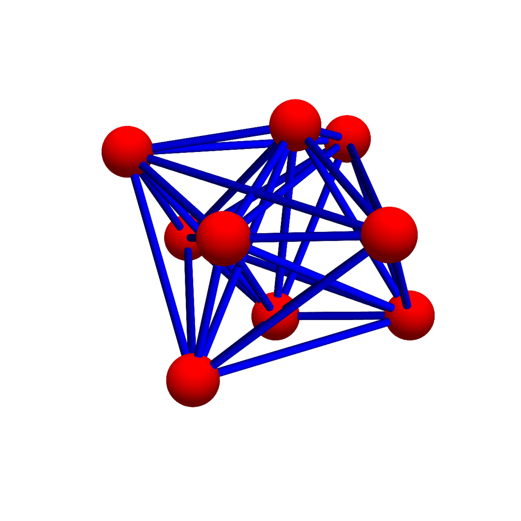
This implies for example that the maximal eigenvalue of is for and the maximal eigenvalue for is for . This is extremal as for all eigenvalue. It also shows that because is the dimensional sphere (cross polytop), that the maximal eigenvalue is . Indeed, the octahedron for example has maximal eigenvalue and the -cell has maximal eigenvalue with multiplicity at least .

11. Questions
Lets finish with some questions.
A) We still have not identified the off diagonal terms
in topological terms, where is the connection graph of a complex.
Having the diagonal terms related to natural sphere index functionals, which are very
closely related to Morse theory, it is likely that also the off diagonal
terms refer to some interesting topological or dynamical notion.
B) Since we have identified two characters and on the sphere group (a homomorphism from the sphere group to the group ), it is natural to ask whether there is more representation theory of the sphere group for which the character are classical characters, represented by a trace of a matrix associated to a sphere. We especially would like to know the collection of all characters. Since the sphere group is discrete, one could take any distance (like the minimal number of vertices or edges to be modified to get from one to an isomorphic image of the other). This is then a topological group which has a Haar measure as discreteness assures that it is locally compact and such that the Haar measure, the counting measure. There are many characters on the sphere group like assigning real numbers to every vertex of a graph and to vertices of . A character is then defined as
Since adding two graphs takes the union of the vertices, this is multiplicative for the additive
group of spheres. But as both and tap into the structure
of the simplices in the graph, it is likely that there are more interesting
examples of characters.
C) The join and multiplication in which the addition is not extended yet, forms a
commutative semiring of type : both addition and multiplication are commutative
monoids, distributivity holds and .
The question of unique prime decomposition in the additive and multiplicative
monoids of abstract finite simplicial complexes is interesting. Maybe the question is more
approachable on submonoids like the sphere monoid. On the multiplicative submonoid of complete graphs,
the prime factorization is the same than on the multiplicative group of natural numbers without .
D) We would also like to be able to compute in the field of fractions defined by the ring and
then do a completion solve equations like leading to or solving with
solution . Both equations can not be solved in the ring
because is an additive prime (every cyclic graph with is an additive prime)
and is a multiplicative prime because every graph with vertices
is a multiplicative prime if is a rational prime.
E) There are interesting questions related to the number theoretically defined prime graphs and prime connection graphs . One can for example try to estimate the Green function values from above. The topology of is linked the Riemann hypothesis as it is directly linked to the growth of the Euler characteristic of by the Mertens connection [25]. The Fredholm characteristic of truncations of truncated prime graphs on the other hand gives a signature, comparing the parity of square free integers which have an even number of prime factors. Such integers correspond to odd-dimensional simplices in the complex. The Green function values for prime graphs, the matrix entries of could contain some interesting number theory.
References
- [1] U. Andrews. Undecidable problems in topology. Online, May 10, 2015.
- [2] R. Bott. Two new combinatorial invariants for polyhedra. Portugaliae Math., 11:35–40, 1952.
- [3] F. Chung and S.-Y. Yau. Discrete Green functions. Journal of Combinatorial Theory (A), 91:191–214, 2000.
- [4] A.V. Evako. Dimension on discrete spaces. Internat. J. Theoret. Phys., 33(7):1553–1568, 1994.
- [5] R. Forman. Morse theory for cell complexes. Adv. Math., page 90, 1998.
- [6] B. Grünbaum. Polytopes, graphs, and complexes. Bull. Amer. Math. Soc., 76:1131–1201, 1970.
- [7] F. Harary. Graph Theory. Addison-Wesley Publishing Company, 1969.
- [8] A. Hatcher. Algebraic Topology. Cambridge University Press, 2002.
- [9] A. Ivashchenko. Contractible transformations do not change the homology groups of graphs. Discrete Math., 126(1-3):159–170, 1994.
- [10] J. Jonsson. Simplicial Complexes of Graphs, volume 1928 of Lecture Notes in Mathematics. Springer, 2008.
- [11]
M. Joswig.
Computing invariants of simplicial manifolds.
https://arxiv.org/abs/math/0401176, 2004. - [12] J. Kahn, M. Saks, and D. Sturtevant. A topological approach to evasiveness. Combinatorica, 4(4):297–306, 1984.
- [13] D.A. Klain and G-C. Rota. Introduction to geometric probability. Lezioni Lincee. Accademia nazionale dei lincei, 1997.
- [14]
O. Knill.
The dimension and Euler characteristic of random graphs.
http://arxiv.org/abs/1112.5749, 2011. - [15]
O. Knill.
A graph theoretical Poincaré-Hopf theorem.
http://arxiv.org/abs/1201.1162, 2012. - [16]
O. Knill.
The McKean-Singer Formula in Graph Theory.
http://arxiv.org/abs/1301.1408, 2012. - [17]
O. Knill.
The Dirac operator of a graph.
http://http://arxiv.org/abs/1306.2166, 2013. - [18]
O. Knill.
Coloring graphs using topology.
http://arxiv.org/abs/1410.3173, 2014. - [19]
O. Knill.
A notion of graph homeomorphism.
http://arxiv.org/abs/1401.2819, 2014. - [20]
O. Knill.
Graphs with Eulerian unit spheres.
http://arxiv.org/abs/1501.03116, 2015. - [21]
O. Knill.
The Künneth formula for graphs.
http://arxiv.org/abs/1505.07518, 2015. - [22]
O. Knill.
Universality for barycentric subdivision.
http://arxiv.org/abs/1509.06092, 2015. - [23]
O. Knill.
Gauss-Bonnet for multi-linear valuations.
http://arxiv.org/abs/1601.04533, 2016. - [24]
O. Knill.
On Fredholm determinants in topology.
https://arxiv.org/abs/1612.08229, 2016. - [25]
O. Knill.
On primes, graphs and cohomology.
https://arxiv.org/abs/1608.06877, 2016. - [26] F.H. Lutz. Triangulated manifolds with few vertices and vertex-transitive group actions. Dissertation, Technische Universitaet Berlin, 1999.
- [27]
F.H. Lutz.
Triangulated manifolds with few vertices and combinatorial manifolds.
https://arxiv.org/abs/math/0506372, 2005. - [28] M. Tsuruga M. Joswig, F.H.Lutz. Sphere recognition: Heuristics and examples. https://arxiv.org/abs/1405.3848, 2015.
- [29] B. Poonen. Undecidable problems: a sampler. In J. Kennedy, editor, Interpreting Gödel: Critical Essays, pages 211–241. Cambridge University Press, 2014.
- [30] J. Rhodes and P.V. Silva. Boolean Representations of Simplicial Complexes and Matroids. Springer Monographs in Mathematics, 2015.
- [31] C.P. Rourke and B.J. Sanderson. Introduction to Piecewise-Linear Topology. Springer Verlag, Berlin, 1982.
- [32] E.H. Spanier. Algebraic Topology. Springer Verlag, 1966.
- [33]
D.A. Spielman.
Bounding eigenvalues.
http://www.cs.yale.edu/homes/spielman/561/lect04-15.pdf, 2009. - [34] J. Stillwell. The word problem and the isomorphism problem for groups. Bulletin (New Series) of the AMS, 6, 1982.
- [35] Wu W-T. Topological invariants of new type of finite polyhedrons. Acta Math. Sinica, 3:261–290, 1953.
- [36] A.H. Wallace. An introduction to Algebraic Topology. Pergamon Press, 1957.
- [37] A.A. Zykov. On some properties of linear complexes. (russian). Mat. Sbornik N.S., 24(66):163–188, 1949.