Generation of attosecond electron beams in relativistic ionization by short laser pulses

To illustrate the theory presented above, we consider the interaction of an intense and circularly polarized laser pulse with He⁺ ions. The latter are one-electron ions, with the atomic number $Z=2$ and the ionization potential of roughly 54 eV. The laser pulse (3) is characterized by the shape functions $f_{j}(\phi)$, for $j=1,2$, defined as

where

for $0<\phi<2\pi$ and it is 0 otherwise. Here, $N_{\rm osc}$ is the number of cycles comprising the pulse, $N_{0}=\sqrt{\frac{8}{3}}N_{\rm osc}$ is a normalization constant which guarantees that the average intensity of the field is independent of the number of cycles [45], whereas $\delta$ and $\delta_{j}$ determine the polarization properties of the pulse. Unless otherwise stated, in the following we consider a three-cycle ($N_{\rm osc}=3$) circularly polarized laser pulse ($\delta_{1}=0$, $\delta_{2}=\pi/2$, and $\delta=\pi/4$) that propagates along the $z$-axis ($\bm{n}={\bm{e}}_{z}$), with the polarization vectors ${\bm{\varepsilon}}_{1}={\bm{e}}_{x}$ and ${\bm{\varepsilon}}_{2}={\bm{e}}_{y}$. The laser carrier frequency, $\omega_{\mathrm{L}}=N_{\mathrm{osc}}\omega$, is equal to $1.5498$ eV.

In Fig. 1, we present the trajectories of the tips of the electric field vector $\bm{\mathcal{E}}(\phi)$ (upper panel) and the vector potential $\bm{A}(\phi)$ (lower panel) in the $xy$-plane for the laser pulse described above. Both curves start and end up at the origin of coordinates and evolve counterclockwise. The parameter $\mathcal{E}_{S}=m_{\mathrm{e}}^{2}c^{3}/|e|$ is the so-called Sauter-Schwinger critical field [61, 62], whereas $A_{S}=m_{\mathrm{e}}c/|e|$. Note that, for the laser field parameters considered in this paper, we have $|\bm{\mathcal{E}}(\phi)|/\mathcal{E}_{\mathrm{S}}\ll 1$. This implicates that, under current conditions, the electron-positron pair creation from vacuum is negligible [45].

In Sec. II we have defined the triply-differential probability distribution of ionization of hydrogen-like ions interacting with short laser pulses [Eq. (15)]. In this case, the initial ground-state wave function is unperturbed at times prior to the interaction with the laser field, independently of its intensity. This allows us to analyze the photoionization of light ions (such as He⁺) by intense laser pulses. In contrast, when the infinite plane-wave approximation is considered (see, e.g., Refs. [63, 64, 65, 54]), the RSFA is restricted to the case of highly charged positive ions interacting with laser fields of moderate intensity. This guarantees that the initial bound state is not heavily distorted by the action of the laser field.

Note also that, when a slowly-varying envelope is used to model the driving laser pulse, the so-called Lambropoulos curse can play a role in the dynamics of photoionization [66]. Namely, it may happen that the hydrogen-like ion is fully ionized during the ramp-up part of the laser pulse, before the field acquires its maximum strength. In contrast, when the envelope varies rapidly, the field reaches values large enough to permit stabilization against ionization in very short time intervals. In this case, the target may survive undisturbed even up to the maximum field strength in the pulse [67].

As described above, our approach offers many advantages as compared to the case when the infinite plane-wave laser field is considered. However, it is still crucial to show that the unitarity of the problem is not violated while applying the approximations described in this paper. In other words, that the total probability of ionization (14) is always less than one. To do so, we calculate below $P_{\mathrm{ion}}$ using the Monte Carlo method.

First, we rewrite Eq. (14) such that

where ${\cal P}({\bm{p}})$ is defined by Eq. (17). To numerically evaluate the energy integral, its upper limit is substituted by a finite value, denoted as $m_{\mathrm{e}}c^{2}+E_{\mathrm{max}}$. It is chosen such that the probability distribution is negligible for photoelectron final energies larger than $E_{\rm max}$. In our calculations, we set $E_{\mathrm{max}}=30$ keV. Now, by introducing the following change of variables,

the total probability of ionization becomes

where we integrate over a unit cube. This expression is now suitable to apply the Monte Carlo method with the uniformly distributed variables $\xi_{i}$ ($i=1,2,3$) (see, e.g., [68, 69]).

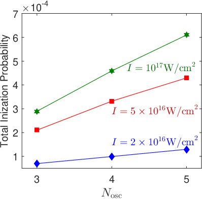
In Fig. 2, we show the total probabilities of photoionization of He⁺ ions by the laser pulse described in the previous Section. The data are for different time-averaged intensities such that $I=2\times 10^{16}$ W/cm² (diamonds), $I=5\times 10^{16}$ W/cm² (squares), and $I=1\times 10^{17}$ W/cm² (stars), and for different number of field cycles, $N_{\rm osc}$. The results were obtained from the Monte Carlo integration of Eq. (22) by considering no less than $10^{6}$ sample points, with the estimated relative standard deviations smaller than 1%. One can clearly see that all calculated probabilities are less than one, which indicates the self-consistency of our treatment. With this in mind, we can study now differential probability distributions of ionization and their properties.

In order to perform the saddle-point analysis, the spin-resolved probability amplitude of ionization (6) is written in terms of the light-cone variables. By doing so, as before, we are able to simplify Eq. (6) to a single integral (see, also Ref. [45]). Namely, we obtain

where $\phi=k^{0}x^{-}$, $M_{\lambda\lambda_{\mathrm{i}}}(\phi)$ is defined by Eq. (7), and it is calculated at the point ${\bm{Q}}={\bm{p}}+(q^{0}-p^{0}){\bm{n}}$. Additionally, the function $G(\phi)$ in Eq. (23) is given by

where

Now, given that the functions $G(\phi)$ and $\bigl[M_{\lambda\lambda_{\mathrm{i}}}(\phi)\bigr]_{\bm{q}=\bm{Q}}$ are sufficiently regular for real $\phi$ whereas $e^{iG(\phi)}$ is a fast oscillating function as compared to the remaining parts of the integrand in (23), the standard saddle-point approximation can be applied. The saddle points are obtained by solving the equation

Among them, the ones that contribute to the integral in Eq. (23), from now on denoted as $\phi_{s}$, are those with $\textrm{Im}\,G(\phi_{s})>0$ (or, equivalently, with ${\rm Im}\,\phi_{s}>0)$. Keeping this in mind, the probability amplitude of ionization in the saddle-point approximation becomes

This expression suggests that the interference-dominated structures in the energy spectra of photoelectrons should appear at regions for which two or more saddle points contribute the most to the above sum. In contrast, if just one of them dominates over a broad range of photoelectron kinetic energies [i.e., if $\textrm{Im}\,G(\phi_{s})$ is considerably smaller compared to the corresponding values of the remaining saddle points], the interference-free structures are expected to be found.

In Fig. 5, we show the imaginary part of $G(\phi_{s})$ as a function of the photoelectron kinetic energy for four saddle points which contribute to the sum in Eq. (27). While the laser field parameters are the same as in Fig. 1 and $\varphi_{\bm{p}}=0.5\pi$ in both panels, two polar angles have been chosen: $\theta_{\bm{p}}=0.46\pi$ (left panel) and $\theta_{\bm{p}}=0.5\pi$ (right panel). Note that, for energies smaller than 60 eV, at least two saddle points contribute significantly to the probability amplitude of ionization (27) as the corresponding $\textrm{Im}\,G(\phi_{s})$ takes the smallest values (cyan and magenta lines). As expected, this region coincides with the interference-dominated low-energy portion of the spectra presented in Fig. 3. Once again, we would like to stress that this is the energy domain beyond the validity of RSFA. For this reason, the analysis above can provide only a qualitative understanding of this particular interference pattern. Fortunately, for the considered laser pulse parameters and in contrast to the high-frequency case investigated in our previous studies [45, 46], the low-energy electrons contribute marginally to the total ionization yield.

The interference-free structures are expected to appear at photoelectron kinetic energies at which an isolated saddle point contributes dominantly in Eq. (27). To illustrate this, we compare Figs. 3 and 5. For $\theta_{\bm{p}}=0.46\pi$, the mid- and high-energy interference-free structures peak in the energy region where $\textrm{Im}\,G(\phi_{s})$ calculated at the dominant saddle points (blue and red curves in the left panel of Fig. 5) reach their minimum values. The same conclusion can be drawn for $\theta_{\bm{p}}=0.5\pi$, with the difference that the high-energy lobe is absent in this case. To understand this we note that $\textrm{Im}\,G(\phi_{s})$, shown as the red and blue curves in the left panel of Fig. 5, have their minima which are by roughly three orders of magnitude smaller than the remaining values of $\textrm{Im}\,G(\phi_{s})$ at the same electron energies. The situation in the right panel is changed as the minimal value of the red curve increases relative to the other values of $\textrm{Im}\,G(\phi_{s})$. Thus, the high-energy structure disappears in the spectrum (see, Fig. 3). Note also that the values of $\textrm{Im}\,G(\phi_{s})$ for the saddle point represented by the red curve seem to change rapidly with the angle $\theta_{\bm{p}}$. Thus, resulting in a sensitivity of the corresponding high-energy structure to the polar angle $\theta_{\bm{p}}$. This is in contrast to the blue curve, which agrees with our earlier observation that the mid-energy lobe in Fig. 3 is less sensitive to the change of $\theta_{\bm{p}}$.

The saddle-point analysis gives a reasonable estimate of the photoelectron time of emission, which is related to ${\rm Re}\phi_{s}$ (see, e.g., Ref. [45]). Specifically, the two saddle points causing the low-energy interference pattern in Fig. 3 are such that, for the electron kinetic energies up to 60 eV, ${\rm Re}\phi_{s}$ changes as 0.28-0.38 (cyan line) and 5.78-5.87 (magenta line). This indicates that the corresponding photoelectrons are ionized at the beginning and at the end of the driving pulse. The mid-energy interference-free structure, on the other hand, peaks at ${\rm Re}\phi_{s}=1.42$ (blue line). These electrons are emitted more towards the middle of the ramp-up part of the pulse. Finally, the high-energy structure has its maximum at ${\rm Re}\phi_{s}=3.7$ (red line). Thus, the corresponding electrons are ionized at roughly maximum value of the laser pulse envelope.

Finally, let us analyze the time-dependent ponderomotive energy of an electron undergoing the quiver motion in a laser field,

For the laser field defined in Fig. 1, $U_{p}$ is plotted in Fig. 6. Hence, we see that photoelectrons which contribute to the mid- and high-energy structures appear in the continuum at times when the ponderomotive energy equals 3.36 keV and 15.41 keV (intersection of the blue and red vertical lines with the curve in Fig. 6), respectively. Note that those values are close to the final photoelectron kinetic energies for which the interference-free distributions acquire their maximum values, i.e., 2.96 keV and 15.5 keV (see the discussion below Fig. 4). This suggests that, for the mid- and high-energy photoelectrons, the ponderomotive energy acquired at the moment of their birth in the continuum is basically transferred into their longitudinal motion. Such an argument cannot be made for low-energy electrons. This discrepancy is actually expected, as the RSFA offers only a qualitative description of photoionization in this part of the spectrum.

Since the RSFA is particularly suitable to describe the highly energetic ionization, in the remaining part of this paper we focus on the high-energy interference-free structure that appears in the photoelectron spectrum of ionization. As we show next, it makes a potential for generating short-in-time electron wave packets.

The spin-resolved probability amplitude of ionization $\mathcal{A}_{\lambda\lambda_{\mathrm{i}}}(\bm{p})$ can be represented as

where the global phase equals $\Phi_{\lambda\lambda_{\mathrm{i}}}(\bm{p})=\mathrm{arg}[\mathcal{A}_{\lambda\lambda_{\mathrm{i}}}(\bm{p})]$. In our further analysis, we will consider electron wave packets propagating in a given space direction determined by the fixed polar and azimuthal angles. For this reason, we will focus below on the energy dependence of the global phase, $\Phi_{\lambda\lambda_{\mathrm{i}}}(\bm{p})$, and the amplitude modulus squared, $|\mathcal{A}_{\lambda\lambda_{\mathrm{i}}}(\bm{p})|^{2}$, proportional to ${\cal P}_{\lambda\lambda_{\rm i}}({\bm{p}})$.

As mentioned above, in order to successfully synthesize an electron wave packet, the global phase of the ionization probability amplitude has to be regular. To quantify this statement, we expand the global phase in a Taylor series around the maximum of the high-energy distribution. Hence, we obtain a constant term, which is physically irrelevant, as well as the linear and quadratic terms, which introduce the time delay and chirp of the electron wave packet, respectively. In order to eliminate the chirp, the derivative of the global phase with respect to the photoelectron energy has to be nearly constant. Furthermore, this derivative should be spin-independent in order to guarantee that the time delay of the electron wave packet does not depend on the initial and final spin degrees of freedom. Note that, in our analysis, the initial spin state is assumed to be projected on the direction of laser pulse propagation, whereas the final spin state is projected on the direction of electron propagation, i.e., it is defined as the helicity.

Fig. 7 shows the derivative of the global phase $\Phi_{\lambda\lambda_{\mathrm{i}}}({\bm{p}})$ with respect to the electron energy (upper panel) and the spin-fixed probabilities of ionization, Eq. (16) (lower panel), as functions of the photoelectron kinetic energy. The laser field parameters are the same as in Fig. 1, whereas the polar and azimuthal detection angles are $\theta_{\bm{p}}=0.46\pi$ and $\varphi_{\bm{p}}=0.5\pi$, respectively. The four curves correspond to different initial and final spin degrees of freedom of the electron $(\lambda,\lambda_{\mathrm{i}})$: $(-,-)$ (dashed red line), $(+,-)$ (dashed cyan line), $(-,+)$ (solid green line), and $(+,+)$ (solid blue line). In the upper panel, all curves overlap, meaning that the derivatives of all phases are spin-independent. We see that these derivatives are nearly constant over a broad range of the final electron kinetic energies. This indicates that no chirp should be observed in the synthesized electron wave packets. Note also that all spin-resolved probabilities shown in the lower panel are comparable, even though the spin-flipping processes are preferable.

Keeping in mind the above discussion, we go back to Eq. (29). Now, if we want to analyze the electron wave packet propagating in a given space direction ${\bm{n}}_{0}$, defined by the polar and azimuthal angles $\theta_{0}$ and $\varphi_{0}$, respectively, we have to introduce in (29) constrains on possible values of ${\cal A}_{\lambda\lambda_{\rm i}}({\bm{p}})$. This can be done by multiplying ${\cal A}_{\lambda\lambda_{\rm i}}({\bm{p}})$ by the properly chosen filter function [45],

In doing so, we create the electron wave packet that propagates in the direction $\bm{n}_{0}$ (with $\theta_{0}=\theta_{\bm{p}}$ and $\varphi_{0}=\varphi_{\bm{p}}$) and contains a range of free-electron energies $E_{\bm{p}}$, namely, $E_{\bm{p}}\in[E_{\mathrm{min}}+m_{\mathrm{e}}c^{2},E_{\mathrm{max}}+m_{\mathrm{e}}c^{2}]$. This reduces the three-dimensional integral in Eq. (29) to the one-dimensional integral only. Thus, the space-time probability amplitude of ionization (29) becomes

where the factor $N_{\mathcal{A}}$ contains all irrelevant constants and $d=\bm{n}_{0}\cdot\bm{x}$ is the electron distance from the parent ion. In the following, we extract from $\tilde{\mathcal{A}}_{\lambda\lambda_{\mathrm{i}}}(t,d)$ the common phase factor $e^{-im_{\mathrm{e}}c^{2}t}$ and define

This time-dependent factor artificially introduces rapid oscillations into the probability amplitude and is irrelevant when calculating probabilities.

Note that $\mathcal{A}_{\lambda\lambda_{\mathrm{i}}}(t,d)$ is a four-component object due to the presence of the free-electron bispinor $u_{\bm{p}\lambda}^{(+)}$. However, in the following, we will concentrate on its first component, $\mathcal{A}_{\lambda\lambda_{\mathrm{i}}}^{(1)}(t,d)$. This is because the space-time probability distributions, defined for each component $j=1,...,4$ as $\mathcal{P}_{\lambda\lambda_{\mathrm{i}}}^{(j)}(t,d)=|\mathcal{A}_{\lambda\lambda_{\mathrm{i}}}^{(j)}(t,d)|^{2}$ and with their maximum normalized to 1, are nearly identical, although the phases of $\mathcal{A}_{\lambda\lambda_{\mathrm{i}}}^{(j)}(t,d)$ are different.

In Fig. 8, we analyze the first component of the ionization probability amplitude (33) for the case when the initial and final electron spins are antiparallel to the laser pulse and the electron propagation directions, respectively; in our notation, $\mathcal{A}^{(1)}_{--}(t,d)$. The results have been obtained for a distance $d=34400a_{0}$ from the parent ion, where $a_{0}$ is the Bohr radius. This particular distance has been chosen such that the electron wave packet has just left the laser pulse, i.e., $\phi=k\cdot x\approx\omega t>2\pi$. Moreover, we have taken $E_{\rm min}=7$ keV and $E_{\rm max}=18$ keV. Note that $\mathcal{A}^{(1)}_{--}(t,d=34400a_{0})$ is a rapidly oscillating function of $t$, which is illustrated in the upper panel by plotting its real part. To show these fast oscillations more clearly, in the lower panel, we plot both real (solid blue) and imaginary (dashed red) parts of $\mathcal{A}^{(1)}_{--}(t,d=34400a_{0})$ in a very short time interval. They present either the sine or cosine type of behavior, that lead to a smooth oscillation-free behavior of the corresponding probability of ionization, $\mathcal{P}^{(1)}_{--}(t,d=34400a_{0})$. The latter is presented in the upper panel as a solid yellow line.

Note that, even after extracting the phase related to the rest energy of the electron from the probability amplitude [cf. Eq. (33)], the latter is still a rapidly oscillating function of time. This follows from the fact that the electron wave packet is built up from the high-energy interference-free portion of the spectrum, for which the condition $E_{\bm{p}}-m_{\mathrm{e}}c^{2}\gg\omega$ is met. Furthermore, we have determined that the resulting electron pulse is very long, as it comprises at least few thousands of oscillations. It is known from laser physics that, for long pulses, the so-called carrier-envelope phase (CEP) is irrelevant. Hence, the same can be expected for the electron diffraction experiments. It is anticipated that the change of CEP for the remaining components of the probability amplitude will not play a significant role either. Finally, we have estimated the width of the electron pulse. As it follows from the upper panel of Fig. 8, just after leaving the laser focus and before spreading in time, the electron pulse width is roughly $\Delta t\approx\pi/(10\omega)\approx 400$ as.

Consider a more intense laser field. It is expected that, for larger intensities of the driving laser field, the resulting high-energy portion of the photoelectron spectrum is shifted towards higher energies. This follows from the fact that the time-dependent ponderomotive energy (28) increases linearly with intensity when the remaining laser field parameters are kept unchanged. Thus, for larger intensities, there is more energy transferred into the longitudinal motion of photoelectrons (see, our analysis in Sec. III.1). It is not obvious, however, how the maximum and the width of this distribution change with increasing the laser field intensity. For this reason, we consider now the case when the photoelectrons are released by the laser field of time-averaged intensity $I=10^{18}$ W/cm². In order to check the consistency of the RSFA for this laser intensity we have estimated, using the Monte Carlo method, that the total ionization probability equals $3.5\times 10^{-4}$ with the standard deviation smaller that $3.5\%$. This calculation was performed assuming that $E_{\mathrm{max}}=200\,\mathrm{keV}$ in Eq. (22).

In the upper panel of Fig. 9, we demonstrate the spin-resolved probability distribution of ionization (16) calculated for the spin configurations $(\lambda,\lambda_{\mathrm{i}})$: $(-,-)$ (solid blue line) and $(-,+)$ (dashed red line) as a function of the photoelectron kinetic energy. While the averaged intensity of the laser pulse is $I=10^{18}$W/cm², its remaining parameters are the same as in Fig. 1. Moreover, the distributions are for the polar and azimuthal detection angles $\theta_{\bm{p}}=0.38\pi$ and $\varphi_{\bm{p}}=0.5\pi$, respectively. As argued in Sec. III, the high-energy structure observed in the ionization probability distribution is very sensitive to the angle $\theta_{\bm{p}}$. By comparing Figs. 4 and 9, we observe that in the current case the high energy photoelectrons are detected at a much smaller polar angle than in Fig. 4. As the driving field is now more intense, it exerts a stronger radiation pressure on the photoelectrons. As a result, the respective probability distribution is shifted towards the direction of propagation of the laser field, i.e., towards smaller $\theta_{\bm{p}}$. Moreover, by comparing $\mathcal{P}_{-\,-}(\bm{p})$ and $\mathcal{P}_{-\,+}(\bm{p})$ for $I=10^{18}$ W/cm² (upper panel of Fig. 9) with the corresponding results for $I=10^{17}$ W/cm² (lower panel of Fig. 7), we see that the maximum of the probability distributions is now shifted by one order of magnitude towards larger photoelectron kinetic energies. The shifting is proportional to the increase of the laser pulse intensity (or the ponderomotive energy). Finally, we observe that the energy bandwidth is wider for the distributions presented in Fig. 9 than for those in Fig. 7. This indicates that the electron pulses build up from these distributions should be shorter for the former. To illustrate this, in the lower panel of Fig. 9, we present the corresponding space-time probability distributions of the photoelectron wave packet $\mathcal{P}_{-\,-}(t,d)$ (solid blue line) and $\mathcal{P}_{-\,+}(t,d)$ (dashed red line), calculated at a distance $d=91000a_{0}$ from the parent ion. Both distributions, defined as

are scaled to the maximum of $\mathcal{P}_{--}(t,d=91000a_{0})$. Now, the temporal width of the photoelectron pulse is roughly $\Delta t\approx 0.025\pi/\omega$, which is around four times shorter than for the case studied in Fig. 7. Note that the time duration of the electron pulse does not scale with the incident laser pulse intensity, as the position of the maximum of the probability distribution does. Actually, the ratio of the energy bandwidth to the energy position at which we observe the maximum decreases with increasing the laser intensity. In other words, the structure, if scaled to the most probable energy of emitted electrons, becomes more narrow. As a consequence, the photoelectron pulse which leaves the laser focus lasts in the current case for roughly 100 as.

Note that the above discussion was based on the plane-wave-fronted pulse approximation for the driving laser field. Next, we will elaborate on the validity of this approximation in relation to the laser pulse parameters used in this paper.

Consider a laser pulse of power $P_{\mathrm{pulse}}=10$ PW, which is focused such that its time-averaged intensity distribution perpendicular to the laser pulse propagation is of the Gaussian form,

Here, $I$ is the laser beam peak intensity whereas $\sigma_{\mathrm{L}}$ determines the spatial size of the focus in the transverse direction. Thus, the total power of the pulse equals

If $I=10^{18}\,\mathrm{W/cm}^{2}$, then

leading to $\sigma_{\mathrm{L}}\approx 4\times 10^{-4}\,\mathrm{m}$. We also estimate that for 10 TW pulses of time-averaged intensity $I=10^{17}\,\mathrm{W/cm}^{2}$, the transverse size of the laser focus $\sigma_{\rm L}$ is by one order of magnitude smaller. In order to test the validity of the plane-wave-fronted pulse approximation, these values should be compared with the distance at which photoelectrons escape from the focus as measured in the perpendicular direction, $d^{\bot}_{\mathrm{escape}}$. Assuming that the position of the parent ion is not influenced by the laser field, due to the ion large mass, we estimate that $d^{\bot}_{\mathrm{escape}}$ is comparable to the separation between the electron wave packet and the ion after leaving the laser focus, as the polar angle of emission is close to $\pi/2$. It is also expected that $d^{\bot}_{\mathrm{escape}}$ is the largest for the most energetic photoelectrons.

Our space-time analysis presented above shows that $d^{\bot}_{\mathrm{escape}}$ does not exceed $10^{5}\,a_{0}\approx 5\times 10^{-6}\,\mathrm{m}$ for the time-averaged intensity $I=10^{18}\,\mathrm{W/cm}^{2}$, and that it decreases for smaller intensities. Hence,

In the current example, $d^{\bot}_{\mathrm{escape}}$ is smaller than the space-size of the laser focus by at least two orders of magnitude, provided that the total power of the pulse is around 10 PW. Note that, for 10 TW pulses and $I=10^{17}\,\mathrm{W/cm}^{2}$, the space-size of the focus is $\sigma_{\mathrm{L}}\approx 4\times 10^{-5}\,\mathrm{m}$ and $d^{\bot}_{\mathrm{escape}}\approx 4\times 10^{4}a_{0}\approx 2\times 10^{-6}\,\mathrm{m}$. This analysis shows that the plane-wave-fronted pulse approximation is suitable for the parameters chosen in the current paper. For lower pulse intensities, our estimations can be improved by increasing the total power of the pulse. On the other hand, for a fixed pulse power, we can extend the validity of the plane-wave-front approximation by designing the laser focus which is not cylindrically symmetric but is elongated in a particular direction. Finally, it is expected that this approximation can break for tighter focusing for which, however, the interference-free supercontinuum does not appear.

References

- [1] R. Srinivasan, V. A. Lobastov, C. -Y. Ruan, and A. H. Zewail, Helv. Chim. Acta 86, 1763 (2003).
- [2] A. H. Zewail, Philos. Trans. R. Soc. London A 363, 315 (2005).
- [3] V. A. Lobastov, R. Srinivasan, and A. H. Zewail, Proc. Natl. Acad. Sci. U.S.A. 102, 7069 (2005).
- [4] A. H. Zewail, Annu. Rev. Phys. Chem. 57, 65 (2006).
- [5] H. Ihee, V. A. Lobastov, U. M. Gomez, B. M. Goodson, R. Srinivasan, C. Y. Ruan, and A. H. Zewail, Science 291, 458 (2001).
- [6] V. A. Lobastov, R. Srinivasan, B. M. Goodson, C. -Y. Ruan, J. S. Feenstra, and A. H. Zewail, J. Phys. Chem. A 105, 11159 (2001).
- [7] R. Srinivasan, J. S. Feenstra, S. T. Park, S. J. Xu, and A. H. Zewail, Science 307, 558 (2005).
- [8] M. Gao et al., Nature 496, 343 (2013).
- [9] J. Yang, J. Beck, C. J. Uiterwaal, and M. Centurion, Nat. Commun. 6, 8172 (2015).
- [10] B. J. Siwick, J. R. Dwyer, R. E. Jordan, and R. J. D. Miller, Science 302, 1382 (2003).
- [11] R. Ernstorfer R, M. Harb, C. T. Hebeisen, G. Sciaini, T. Dartigalongue, and R. J. D. Miller, Science 323, 1033 (2009).
- [12] G. Sciaini, M. Harb, S.G. Kruglik, T. Payer, C.T. Hebeisen, F.-J. Meyer Zu Heringdorf, M. Yamaguchi, M. Horn-von Hoegen, R. Ernstorfer, and R. J. D. Miller, Nature 458, 56 (2009).
- [13] N. Gedik, D.-S. Yang, G. Logvenov, I. Bozovic, and A.H. Zewail, Science 316, 425 (2007).
- [14] P. Baum, D.-S. Yang, and A. H. Zewail, Science 318, 788 (2007).
- [15] M. Aidelsburger, F. O. Kirchner, F. Krausz, and P. Baum, Proc. Natl. Acad. Sci. U.S.A. 107, 19714 (2010).
- [16] P. Hommelhoff, Y. Sortais, A. Aghajani-Talesh, and M. A. Kasevich, Phys. Rev. Lett. 96, 077401 (2006).
- [17] P. Hommelhoff, C. Kealhofer, and M. A. Kasevich, Phys. Rev. Lett. 97, 247402 (2006).
- [18] C. Ropers, D. R. Solli, C. P. Schulz, C. Lineau, and T. Elsaesser, Phys. Rev. Lett. 98, 043907 (2007).
- [19] M. Schenk, M. Krüger, and P. Hommelhoff, Phys. Rev. Lett. 105, 257601 (2010).
- [20] M. Krüger, M. Schenk, and P. Hommelhoff, Nature 475, 78 (2011).
- [21] J. Kupersztych, P. Monchicourt, and M. Raynaud, Phys. Rev. Lett. 86, 5180 (2001).
- [22] S. E. Irvine, A. Dechant, and A. Y. Elezzabi, Phys. Rev. Lett. 93, 184801 (2004).
- [23] S. E. Irvine and A. Y. Elezzabi, Phys. Rev. A 73, 013815 (2006).
- [24] S. R. Greig and A. Y. Elezzabi, Opt. Express 22, 29092 (2014).
- [25] S. R. Greig and A. Y. Elezzabi, Sci. Rep. 6, 19056 (2016).
- [26] B. J. Claessens, S. B. van der Geer, G. Taban, E. J. D. Vredenbregt, and O. J. Luiten, Phys. Rev. Lett. 95, 164801 (2005).
- [27] G. Taban, M.P. Reijnders, B. Fleskens, S. B. van der Geer, O. J. Luiten, and E. J. D. Vredenbregt, Europhys. Lett. 91, 46004 (2010).
- [28] W. J. Engelen, M. A. van der Heijden, D. J. Bakker, E. J. D. Vredenbregt, and O. J. Luiten, Nat. Commun. 4, 1693 (2013).
- [29] B. J. Siwick, J. R. Dwyer, R. E. Jordan, and R. J. D. Miller, J. Appl. Phys. 92, 1643 (2002).
- [30] A. Paarmann, M. Gulde, M. Müller, S. Schäfer, S. Schweda, M. Maiti, C. Xu, T. Hohage, F. Schenk, C. Ropers, and R. Ernstorfer, J. Appl. Phys. 112, 113109 (2012).
- [31] P. Baum and A. H. Zewail, Proc. Natl. Acad. Sci. U.S.A. 104, 18409 (2007).
- [32] P. Baum and A. H. Zewail, Chem. Phys. 366, 2 (2009).
- [33] A. H. Zewail, Science 328, 187 (2010).
- [34] G. Sciaini and R. J. D. Miller, Rep. Prog. Phys. 74, 096101 (2011).
- [35] P. Baum, Chem. Phys. 423, 55 (2013).
- [36] A. Gliserin, M. Walbran, F. Krausz, P. Baum, Nat. Commun. 6, 8723 (2015).
- [37] E. Fill, L. Veisz, A. Apolonski, and F. Krausz, New J. Phys. 8, 272 (2006).
- [38] S. A. Hilbert, C. Uiterwaal, B. Barwick, H. Batelaan, and A. H. Zewail, Proc. Natl. Acad. Sci. U.S.A. 106, 10558 (2009).
- [39] A. Gliserin, A. Apolonski, F. Krausz, and P. Baum, New J. Phys. 14, 073055 (2012).
- [40] P. Hansen, C. Baumgarten, H. Batelaan, and M. Centurion, Appl. Phys. Lett. 101, 083501 (2012).
- [41] H.-C. Shao and A. F. Starace, Phys. Rev. Lett. 105, 263201 (2010).
- [42] H.-C. Shao and A. F. Starace, Phys. Rev. A 87, 050701(R) (2013).
- [43] H.-C. Shao and A. F. Starace, Phys. Rev. A 88, 062711 (2013).
- [44] H.-C. Shao and A. F. Starace, Phys. Rev. A 90, 032710 (2014).
- [45] K. Krajewska and J. Z. Kamiński, Phys. Rev. A 94, 013402 (2016).
- [46] F. Cajiao Vélez, J. Z. Kamiński, and K. Krajewska, arXiv:1612.09293; J. Phys.: Conf. Ser. (to be published).
- [47] https://eli-laser.eu/.
- [48] http://www.xcels.iapras.ru/.
- [49] Ch. Varin and M. Piché, Phys. Rev. E 74, 045602R (2006).
- [50] T. van Oudheusden, E. F. de Jong, S. B. van der Geer, W. P. E. M. Op’t Root, O. J. Luiten, and B. J. Siwick, J. Appl. Phys. 102, 093501 (2007).
- [51] L. Veisz, G. Kurkin, K. Chernov, V. Tarnetsky, A. Apolonski, F. Krausz, and E. Fill, New J. Phys. 9, 451 (2007).
- [52] T. van Oudheusden, P. L. E. M. Pasmans, S. B. van der Geer, M. J. de Loos, M. J. van der Wiel, and O. J. Luiten, Phys. Rev. Lett. 105, 264801 (2010).
- [53] R. P. Chatelain, V. R. Morrison, C. Godbout, and B. J. Siwick, Appl. Phys. Lett. 101, 081901 (2012).
- [54] H. R. Reiss, J. Opt. Soc. Am. B 7, 574 (1990).
- [55] J. D. Bjorken and S. D. Drell, Relativistic Quantum Mechanics (McGraw-Hill, New York, 1964).
- [56] D. M. Wolkow, Z. Phys. 94, 250 (1935).
- [57] F. Ehlotzky, K. Krajewska, and J. Z. Kamiński, Rep. Prog. Phys. 72, 046401 (2009).
- [58] A. Di Piazza, C. Müller, K. Z. Hatsagortsyan, and C. H. Keitel, Rev. Mod. Phys. 84, 1177 (2012).
- [59] K. Krajewska and J. Z. Kamiński, Phys. Rev. A 85, 062102 (2012).
- [60] K. Krajewska and J. Z. Kamiński, Phys. Rev. A 86, 052104 (2012).
- [61] F. Sauter, Z. Phys. 69, 742 (1931).
- [62] J. Schwinger, Phys. Rev. 82, 664 (1951).
- [63] M. Klaiber, E. Yakaboylu, and K. Z. Hatsagortsyan, Phys. Rev. A 87, 023418 (2013).
- [64] M. Klaiber and K. Z. Hatsagortsyan, Phys. Rev. A 90, 063416 (2014).
- [65] E. Yakaboylu, M. Klaiber, and K. Z. Hatsagortsyan, Phys. Rev. A 91, 063407 (2015).
- [66] P. Lambropoulos, Phys. Rev. Lett. 55, 2141 (1985).
- [67] M. V. Fedorov and S. M. Fedorov, Opt. Express 3, 271 (1998).
- [68] J. Z. Kamiński, K. Krajewska, and F. Ehlotzky, Phys. Rev. A 74, 033402 (2006).
- [69] K. Krajewska, C. Müller, and J. Z. Kamiński, Phys. Rev. A 87, 062107 (2013).
- [70] K. Krajewska and J. Z. Kamiński, Phys. Rev. A 92, 043419 (2015).
- [71] K. Krajewska and J. Z. Kamiński, Laser Phys. Lett. 11, 035301 (2014).
- [72] K. Krajewska, M. Twardy, and J. Z. Kamiński, Phys. Rev. A 89, 032125 (2014).
- [73] K. Krajewska and J. Z. Kamiński, Phys. Rev. A 90, 052108 (2014).
- [74] M. J. A. Jansen and C. Müller, Phys. Lett. B 766, 71 (2017).
- [75] A. Angioi, F. Mackenroth, and A. Di Piazza, Phys. Rev. A 93, 052102 (2016).
- [76] M. Kalashnikov, A. Andreev, K. Ivanov, A. Galkin, V. Korobkin, M. Romanovsky, O. Shiryaev, M. Schnuerer, J. Braenzen, V. Trofimov, Laser Part. Beams 33, 361 (2015).
- [77] K. Krajewska and J. Z. Kamiński, Phys. Lett. A 380, 1247 (2016).