KIAS-P17012
Discriminating leptonic Yukawa interactions with doubly charged scalar at the ILC
Abstract
We explore discrimination of two types of leptonic Yukawa interactions associated with Higgs triplet, , and with singlet doubly charged scalar, . These interactions can be distinguished by measuring the effects of doubly charged scalar boson exchange in the processes at polarized electron-positron colliders. We study a forward-backward asymmetry of scattering angular distribution to estimate the sensitivity for these effects at the ILC. In addition, we investigate prospects of upper bounds on the Yukawa couplings by combining the constraints of lepton flavor violation processes and the processes at the LEP and the ILC.
I Introduction
Doubly charged scalar bosons sometimes play an important role in building models which explain neutrino masses and mixing. One of the representative scenarios is called type-II seesaw mechanism [1, 2, 3] in which an isospin triplet scalar field is introduced. Since has hypercharge 11 1 Here we apply the convention for hypercharge where electric charge is given by and the diagonal generator of gauge symmetry has eigenvalues for a triplet. , it contains an electrically neutral (), singly-charged (), and doubly charged () bosons, and directly couples to the isospin-doublet leptons at tree level via . The neutrino mass matrix is induced after develops a vacuum expectation value (VEV) which violates the lepton number by two. To achieve the smallness of neutrino masses, the VEV of or/and the Yukawa couplings have to be small.22 2 Notice here that the upper bound on the triplet VEV is about a few GeV, which is derived by the fact that the deviation of the electroweak rho parameter from unity is severely constrained by experimental measurements. Interactions of and provide promising signals of doubly (singly) charged bosons at collider experiments. Notice here that these interactions are associated with leptons with left-handed chirality.
Another type of interaction is often employed in radiative seesaw models, such as the Zee-Babu model [4], in which doubly (singly) charged scalar bosons, , are introduced as an isospin singlet; the topology of neutrino mass generating diagram was shown in Ref. [3] for the first time. Then directly couples to the isospin-singlet leptons at tree level via 33 3 This type of interaction also appears in left-right symmetric models [5, 6, 7, 8, 9, 10] associated with triplet scalar which couples to right-handed fermions. , which is also a source of lepton number violation by two unit. The neutrino mass matrix is generated at two-loop level via several terms related to the doubly (singly) charged bosons after the electroweak symmetry breaking by the standard-model (SM) Higgs boson where we can naturally consider models with Yukawa coupling and/or new particles whose masses are TeV inside the loops. The interaction is associated with leptons with right-handed chirality in contrast to the type-II seesaw scenario.
These two types of Yukawa interaction would also appear in many other neutrino mass models as a source of lepton number violation. Thus it is important to analyze the interactions of doubly charged scalar bosons and charged leptons to discriminate models of neutrino mass generation [11]. Searches for the doubly charged scalar bosons have been performed in the past and current collider experiments, and the most severe constraint is obtained by the same-sign di-lepton resonance searches at the LHC [12, 13, 14, 15, 16, 17, 18]. In addition, multi lepton signals are discussed including doubly charged Higgs production associated with singly charged Higgs [19, 20]. Assuming a large branching ratio of a certain di-lepton channel, the most stringent bound on the mass of doubly charged scalar bosons varies from 770 GeV to 870 GeV depending on the models and the decay branching ratio, which is obtained from the latest LHC data [18].
The two bosons have also different interaction with the electroweak gauge bosons. Namely the doubly charged scalar boson of triplet models can couple to a pair of charged gauge bosons, ’s, at tree level. The decay branching ratio to the same-sign can be large if the triplet VEV is as large as MeV depending on the mass itself. Thus the search for such events provides an unique signature of the triplet model [21, 22, 23]. Production of doubly charged scalar bosons via the -fusion process is also expected in the triplet-like models, such as the Georgi-Machacek model [24], which realize a large triplet VEV to make the production cross section sizable [25, 26, 27].
In this paper, we study the effects of the doubly charged scalar boson exchange in processes [29, 28] at future lepton colliders. We consider the initial-state polarization to discriminate the two types of the interactions, and study the bounds of their masses and couplings probed at the future international linear collider (ILC) experiment [30]. Furthermore, we discuss prospects of constraining model parameter space by combining the current and future constraints of lepton flavor violating (LFV) processes as well as the constraints at the LEP experiment [31].
The paper is organized as follows. In Sec. II, we discuss constraints from LFV processes. In Sec. III, we consider the effects of doubly charged scalar bosons to the processes at lepton colliders, and study the constraints on the mass and couplings of these bosons by using the forward-backward asymmetry. In Sec. IV we summarize the constraints and prospects of future bounds on the relevant effective couplings with numerical analysis. Sec. V is devoted for conclusions and discussions.
II LFV processes
In this section, constrains from LFV processes are reviewed where we summarize bounds of LFV processes on the two representative terms, in Higgs triplet models, and in Zee-Babu type models.
II.1 LFV processes in a Higgs triplet model
We discuss the LFV processes in a Higgs triplet model induced by following relevant Lagrangian44 4 A notation in this paper is different from that in some papers such as Ref. [32] where is replaced by in Eq. (II.1). :
| (II.1) | ||||
where is a symmetric Yukawa coupling matrix, , whose indices run over (, , ), and is the second Pauli matrix. Thus the doubly charged Higgs interactions are left-handed type in this case.


These Yukawa interactions induce LFV processes and at tree and one-loop levels, respectively, through virtual and mediations as shown in Fig. 1. Then one obtains the constraints on the combination of and masses of and by comparing the measured branching ratios (BRs) of these LFV processes and those of model predictions. Table 1 summarizes the upper limits of the BRs and the corresponding constraints for the three-body decay processes [33], and Table 2 summarizes the constraints from the upper limit of BR for given by the recent MEG experiment [34], and from the upper limits of BRs for , given by Ref. [35] applying results in Ref. [32] 55 5 The constraints are obtained from the analysis in the reference where we take into account the difference of notations mentioned in footnote 4..
| Upper limits of BRs | Constraints on |
|---|---|
| Upper limits of BRs | Constraints |
|---|---|
The Yukawa interactions also induce conversion via the same one-loop diagrams which induce the process. The conversion rate is approximately given by the following form [36]:
| (II.6) |
where , and nucleus-dependent parameters , , as well as the bounds on are listed in Table 3. Then the resultant upper bounds for the Yukawa coupling are estimated once boson masses are fixed. Moreover future experimental bounds for can be estimated [37, 38].
II.2 LFV processes with interaction
We proceed the same discussion as the Higgs triplet model in the case of
| (II.7) |
where is also a symmetric Yukawa matrix; therefore,. Thus the doubly charged Higgs interactions are right-handed type in this case. Here notice that the constraint of the three-body decay are the same as that for the Higgs triplet model by replacing . On the other hand, the formulas for the constraint of are different from those in the Higgs triplet case due to the absence of the singly charged scalar boson. Then the constraints on the combination of and the mass of [48] are summarized in Table 4.
| Upper limits of BRs | Constraints |
|---|---|
The constraint of conversion is also given by the following form:
| (II.8) |
where , , and the bounds on are given previously.
III Collider Physics
Here we discuss effects of the two types of Yukawa interactions for charged leptons and a doubly charged scalar boson in collider experiments. The interactions of Eqs. (II.1) and (II.7) contribute to the processes of where the doubly charged scalar bosons propagate in the -channel [29]. By taking the doubly charged scalar bosons as a heavy particle, we obtain the following effective Lagrangians from the Higgs triplet and Zee-Babu type interactions respectively:
| (III.1) | ||||
| (III.2) |
where is the Kronecker delta, we used the Fierz transformation to get the relevant form of the interactions, and is a factor coming from the symmetric structure of the Yukawa couplings: for . Thus the scale parameters and original parameters in the models are related by:
| (III.3) |
Applying effective interactions Eq. (III.1) and (III.2), we then show constraints by using LEP results and prospects of exploring these interactions at the ILC.
Here, we emphasize merits of studying these scattering processes to constrain the effective interactions, which are (1) a particular coupling can be investigated in each process while combinations of different couplings are constrained by LFV processes, (2) right-handed and left-handed couplings can be clearly distinguished by using the polarized electron and positron beams.
III.1 The constraints from LEP experiment
The LEP constraints on the effective interactions are given in Ref. [31] in terms of which are obtained by fitting the scattering angular distribution in processes. We then rewrite the constraints for by the parameters in the original models using the relation Eq. (III.3). As a result the following constraints for each flavor are given in Higgs triplet case:
| (III.4) |
where we have applied Table 3.15 of Ref. [31] taking only one of the Yukawa couplings to be non-zero. In a similar way, one obtains the following constraints for the interaction:
| (III.5) |
III.2 The constraints from the ILC
Here we discuss the constraints on the effective interactions Eq. (III.1) and (III.2) at the ILC. At the ILC, doubly charged scalar effects are studied in
| (III.6) | ||||
| (III.7) | ||||
| (III.8) |
where we assign momenta and helicities of initial (final)-state leptons . In each process, an additional diagram via the effective 4-point vertex is added to the SM diagrams.
Applying Eq. (III.1) and (III.2), helicity amplitudes for the first process are given as
| (III.9) | ||||
| (III.10) | ||||
| (III.11) | ||||
| (III.12) |
where , , , , and is the scattering polar angle. Azimuthal angle dependence is neglected. with being the QED coupling constant, and where is the weak mixing angle. The helicity amplitudes for the second and third processes are obtained by removing terms with and and replacing .
The differential cross-section for purely-polarized initial-state () is given as
| (III.13) |
The case for the partially-polarized initial-state with the degree of polarization for the electron beam and for the positron beam is given as
| (III.14) |
Polarized cross sections are useful to distinguish the left- and right-handed type interactions; e.g. a case of is more sensitive to and less sensitive to . For the realistic values at the ILC, we consider the following two cases [30]:
| (III.15) | ||||
| (III.16) |
defining polarized cross sections .
| [TeV] | [TeV] | [TeV] | [TeV] | [TeV] | [TeV] | |
|---|---|---|---|---|---|---|
| 42 | 12 | 63 | 17 | 60 | 16 | |
| 11 | 39 | 14 | 60 | 13 | 56 | |
| [TeV] | [TeV] | [TeV] | [TeV] | [TeV] | [TeV] | |
| 21 | 6 | 30 | 8 | 28 | 8 | |
| 6 | 21 | 7 | 28 | 6 | 26 | |


To study the sensitivity to the doubly charged scalar effects, we consider the measurement of a forward-backward asymmetry at the ILC, which is defined as
| (III.17) |
where
| (III.18) | ||||
| (III.19) |
is an integrated luminosity, is an efficiency of observing the events, and a kinematical cut is chosen to maximize the sensitivity. For simplicity, we assume for and , while for [43]. We take for , and for and .
| [TeV] | [TeV] | [TeV] | [TeV] | [TeV] | [TeV] | |
|---|---|---|---|---|---|---|
| 35 | 10 | 53 | 14 | 50 | 13 | |
| 9 | 33 | 12 | 50 | 11 | 47 | |
| [TeV] | [TeV] | [TeV] | [TeV] | [TeV] | [TeV] | |
|---|---|---|---|---|---|---|
| 59 | 18 | 90 | 24 | 85 | 23 | |
| 16 | 55 | 21 | 85 | 20 | 80 | |
A statistical error of the asymmetry for the SM is given by
| (III.20) |
where the values in the RHS are obtained by taking . We estimate the sensitivity to the scale ( confidence level) by requiring
| (III.21) |
For GeV with an integrated luminosity fb-1, we get the upper limit of which could be probed by using and as summarized in Table 5; here we take one of is finite value and others are set to be infinity assuming corresponding Yukawa coupling is zero. We thus find that the sensitivity to the scales of two types of the effective interaction is significantly different for each polarized cross section. Therefore the type of the interaction can be distinguished by comparing the results for different beam polarizations. To explicitly see the discrimination, we show for process as a function of in left(right) plot of Fig. 2 which is compared with and statistical errors for the SM. We clearly see that the left(right)-handed type interaction leads . In addition, we can discover the new physics effect with significance when a value of is not too large, and can distinguish a type of interaction by comparing and .
The scales we estimated for the case of the final-state are compared with those given in Ref. [44] where simulation studies of discovering new physics effects by fitting the scattering angular distribution are performed. We find that their method improves the achievable scale by about - from our study using . Therefore, we may expect such factors of improvement for the cases of and final-states too. Detailed study should be performed by including effects of beam-energy spectrum, electroweak higher-order corrections, and detector resolutions.
In addition, we present the results for different and in Tables 6, 7 and 8. The upper limit of can reach 85(90) TeV for TeV with fb-1. Thus we obtain constraints on the couplings by .




IV Summary of the constraints with numerical analysis
In this section, we summarize the constraints on the couplings and by combining bounds from the LFV processes and the processes. We consider sets of Yukawa couplings in the range of by generating random numbers of in in the range of . Then, we impose the constraints of LFV processes. In the following, we consider fixed TeV, for simplicity.
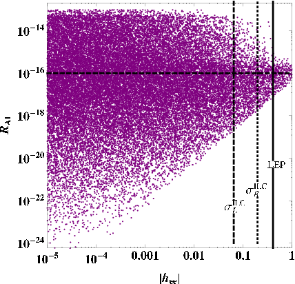
The upper (lower)-left plot in Fig. 3 shows the allowed region in the - plane while the upper (lower)-right plot shows that in the - plane. In these plots, each red (purple) point indicates one set of generated Yukawa couplings which satisfies the constraints of LFV processes. We note that; (I) absence of points in lower-right region in each plot is due to the lower bound in generating Yukawa couplings , therefore artificial since the predictions on can be arbitrary small by setting small except . (II) constraints of LFV processes are slightly stronger on than because of contribution from the singly charged scalar. We also indicate the LEP bound and the ILC bound depending on polarized cross sections for the case of TeV and fb-1; the constraint is obtained by imposing Eq. (III.21) where we apply Eq. (III.3) to extract bounds for Yukawa couplings. In contrast to the constrains from LFV, we can obtain constraints on a single Yukawa coupling from the collider experiments. Note also that the constraints from is stronger(weaker) than the other for left(right)-handed type interaction as we discussed in previous section. In addition, the future upper bound of the conversion rate is shown by horizontal dashed line. We find that within the parameter sets we generated ( most of the regions where a signal can be seen at the ILC can be checked by the conversion experiment. The ILC signal in the absence of the conversion signal may indicate a hierarchical structure of the Yukawa matrix.
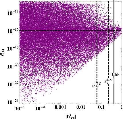
The upper (lower)-left plot in Fig. 4 shows the allowed region in - plane while the upper (lower)-right plot shows that in - plane. In these plots, each red point corresponds to one of the generated Yukawa coupling sets which satisfy the constraints from LFV processes. A lower density of points indicates that a larger fraction of generated parameter sets are excluded in that region by the constraints of the LFV processes other than . The upper-right regions in the upper (lower) plots are explicitly excluded by the LFV processes . The LEP bounds are shown by black lines indicating and while the ILC bounds by polarized cross section are shown by dashed (dotted) lines indicating and for the case of TeV and fb-1. These bounds are simply scaled as for the different mass value of the doubly charged scalar bosons.
Here we comment on the Yukawa couplings , and . These couplings are not shown in Figs. 3 and 4 explicitly, since they are not directly constrained by lepton collider experiments in our analysis. However they are constrained from the LFV processes as Tables 1, 2 and 4 combining with other couplings. Then we have implicitly included LFV constraints when we run these parameters in generating Figs. 3 and 4. We also note that flavor-violating scattering processes, , can also be investigated at the ILC [45] which will test combinations of the Yukawa couplings such as .
Note that including fit to neutrino oscillation data LFV and LHC physics are investigated for effective theory obtained by integrating out the SM charged-leptons, an singlet singly-charged scalar, and doubly-charged scalar in Ref. [46]. Then the relative size of Yukawa couplings are constrained from neutrino oscillation data and LHC can search for doubly charged Higgs where the signal is determined by branching ratio for decay process . If we find the signal of doubly charged Higgs at the LHC, the relative magnitude of Yukawa couplings can be investigated via branching ratio. One advantage of our analysis for lepton collider is that we can constrain absolute magnitude of some Yukawa couplings as we discussed above.
In our analysis we have not included fitting with neutrino oscillation data to investigate direct constraints on the Yukawa couplings associated with doubly charged scalar in general. If we take into account neutrino oscillation data, relative size of Yukawa couplings are constrained; absolute sizes of Yukawa couplings are controlled by VEV of triplet in type-II seesaw case and by mass scale inside loop diagram in Zee-Babu type models. For example, in type-II seesaw case we obtain the relation for normal(inverted) ordering neutrino mass [47]. Also some constraints on relative sizes of Yukawa couplings can be obtained in Zee-Babu model from fitting to neutrino oscillation data [48], which are weaker than the case of type-II seesaw since we have freedom to tune Yukawa couplings associated with singly charged scalar field. Therefore combining neutrino oscillation data and tests for effective operators at the ILC, we can further explore the parameter region for Yukawa couplings by specifying neutrino mass generation mechanism.
V Conclusions
We have explored discrimination of two types of leptonic Yukawa interactions associated with a Higgs triplet or -singlet doubly charged scalar boson where the former one appears in realization of type-II seesaw mechanism for neutrino mass generation and the latter one appears in Zee-Babu type models of radiative neutrino mass generation.
First we have reviewed the constraints from lepton flavor violating (LFV) processes for each type of Yukawa interactions where , and conversion processes are discussed. Next we have shown that these interactions can be distinguished at the ILC by measuring the difference of the scattering angular distribution in the processes with polarized electron and positron beams due to the chirality difference of the interactions. The forward-backward asymmetry in the scattering angular distribution has been investigated to obtain the upper bound of these couplings. Finally we have shown prospects of bounds on the model parameter space by combining the constraints of future LFV processes and the processes at the ILC.
Acknowledgments
H. O. is sincerely grateful for all the KIAS members.
References
- [1] M. Magg and C. Wetterich, Phys. Lett. B 94, 61 (1980); G. Lazarides, Q. Shafi and C. Wetterich, Nucl. Phys. B 181, 287 (1981); R. N. Mohapatra and G. Senjanovic, Phys. Rev. D 23, 165 (1981); E. Ma and U. Sarkar, Phys. Rev. Lett. 80, 5716 (1998).
- [2] W. Konetschny and W. Kummer, Phys. Lett. B 70, 433 (1977); J. Schechter and J. W. F. Valle, Phys. Rev. D 22, 2227 (1980); S. M. Bilenky, J. Hosek and S. T. Petcov, Phys. Lett. B 94, 495 (1980).
- [3] T. P. Cheng and L. -F. Li, Phys. Rev. D 22, 2860 (1980);
- [4] A. Zee, Nucl. Phys. B 264, 99 (1986); K. S. Babu, Phys. Lett. B 203, 132 (1988).
- [5] R. N. Mohapatra and J. C. Pati, Phys. Rev. D 11, 2558 (1975).
- [6] J. C. Pati and A. Salam, Phys. Rev. D 10, 275 (1974) [Phys. Rev. D 11, 703 (1975)].
- [7] G. Senjanovic and R. N. Mohapatra, Phys. Rev. D 12, 1502 (1975).
- [8] G. Senjanovic, Nucl. Phys. B 153, 334 (1979).
- [9] R. N. Mohapatra and G. Senjanovic, Phys. Rev. Lett. 44, 912 (1980).
- [10] R. N. Mohapatra and G. Senjanovic, Phys. Rev. D 23, 165 (1981).
- [11] H. Sugiyama, K. Tsumura and H. Yokoya, Phys. Lett. B 717, 229 (2012).
- [12] G. Aad et al. [ATLAS Collaboration], Phys. Rev. D 85, 032004 (2012).
- [13] G. Aad et al. [ATLAS Collaboration], JHEP 1503, 041 (2015).
- [14] The ATLAS collaboration [ATLAS Collaboration], ATLAS-CONF-2016-051.
- [15] S. Chatrchyan et al. [CMS Collaboration], Eur. Phys. J. C 72, 2189 (2012).
- [16] S. Biondini and O. Panella, Phys. Rev. D 92, no. 1, 015023 (2015)
- [17] K. S. Babu and S. Jana, arXiv:1612.09224 [hep-ph].
- [18] The ATLAS collaboration [ATLAS Collaboration], ATLAS-CONF-2017-053.
- [19] A. G. Akeroyd, C. W. Chiang and N. Gaur, JHEP 1011, 005 (2010)
- [20] CMS Collaboration [CMS Collaboration], CMS-PAS-HIG-16-036.
- [21] S. Kanemura, K. Yagyu and H. Yokoya, Phys. Lett. B 726, 316 (2013).
- [22] S. Kanemura, M. Kikuchi, K. Yagyu and H. Yokoya, Phys. Rev. D 90, no. 11, 115018 (2014).
- [23] S. Kanemura, M. Kikuchi, H. Yokoya and K. Yagyu, PTEP 2015, 051B02 (2015).
- [24] H. Georgi and M. Machacek, Nucl. Phys. B 262, 463 (1985).
- [25] C. W. Chiang, T. Nomura and K. Tsumura, Phys. Rev. D 85, 095023 (2012).
- [26] B. Dutta, R. Eusebi, Y. Gao, T. Ghosh and T. Kamon, Phys. Rev. D 90, 055015 (2014).
- [27] V. Khachatryan et al. [CMS Collaboration], Phys. Rev. Lett. 114, no. 5, 051801 (2015).
- [28] E. Eichten, K. D. Lane and M. E. Peskin, Phys. Rev. Lett. 50 (1983) 811.
- [29] M. L. Swartz, Phys. Rev. D 40 (1989) 1521.
- [30] H. Baer et al., arXiv:1306.6352 [hep-ph].
- [31] S. Schael et al. [ALEPH and DELPHI and L3 and OPAL and LEP Electroweak Collaborations], Phys. Rept. 532, 119 (2013).
- [32] H. Okada, Y. Orikasa and K. Yagyu, arXiv:1510.00799 [hep-ph].
- [33] A. G. Akeroyd, M. Aoki and H. Sugiyama, Phys. Rev. D 79, 113010 (2009).
- [34] A. M. Baldini et al. [MEG Collaboration], Eur. Phys. J. C 76, no. 8, 434 (2016).
- [35] J. Adam et al. [MEG Collaboration], Phys. Rev. Lett. 110, 201801 (2013).
- [36] R. Alonso, M. Dhen, M. B. Gavela and T. Hambye, JHEP 1301, 118 (2013)
- [37] R. J. Barlow, Nucl. Phys. Proc. Suppl. 218, 44 (2011).
- [38] E. V. Hungerford [COMET Collaboration], AIP Conf. Proc. 1182, 694 (2009).
- [39] C. Dohmen et al. [SINDRUM II Collaboration], Phys. Lett. B 317, 631 (1993).
- [40] W. H. Bertl et al. [SINDRUM II Collaboration], Eur. Phys. J. C 47, 337 (2006).
- [41] W. Honecker et al. [SINDRUM II Collaboration], Phys. Rev. Lett. 76, 200 (1996).
- [42] J. Herrero-Garcia, M. Nebot, N. Rius and A. Santamaria, Nucl. Phys. B 885, 542 (2014).
- [43] T. H. Tran, V. Balagura, V. Boudry, J. C. Brient and H. Videau, Eur. Phys. J. C 76 (2016) no.8, 468.
- [44] S. Riemann, LC-TH-2001-007.
- [45] G. C. Cho and H. Shimo, arXiv:1612.07476 [hep-ph].
- [46] S. F. King, A. Merle and L. Panizzi, JHEP 1411, 124 (2014) [arXiv:1406.4137 [hep-ph]].
- [47] P. Fileviez Perez, T. Han, G. y. Huang, T. Li and K. Wang, Phys. Rev. D 78, 015018 (2008) [arXiv:0805.3536 [hep-ph]].
- [48] J. Herrero-Garcia, M. Nebot, N. Rius and A. Santamaria, Nucl. Phys. B 885, 542 (2014) [arXiv:1402.4491 [hep-ph]].