Constraints on neutrino masses from Lyman-alpha forest power spectrum with BOSS and XQ-100

XQ-100, “Quasars and their absorption lines: a legacy survey of the high-redshift universe with VLT/XSHOOTER”, is one of the large programmes of the European Southern Observatory López et al. (2016). The survey consists of a homogeneous and high-quality sample of 100 echelle spectra of quasars at redshifts $z\simeq 3.5-4.5$. The quasars were observed with full spectral coverage from $3\,150$ to $25\,000\,\AA$, at a resolving power ranging from $\sim 4\,000$ to $7\,000$, depending on wavelength.

We use both the XQ-100 raw data and the XQ-100 Science Data Products (SDP) released at http://archive.eso.org/eso/eso_archive_main.html and http://archive.eso.org/wdb/wdb/adp/phase3_main/form, respectively. The main part of our work relies on the SDP spectra; the raw spectra are only exploited for the study and validation of the spectrograph resolution, see Sec. 2.3.

The region of interest for this study, the Ly$\alpha$ forest, is covered by the UVB $(3\,150-5\,600\,\AA)$ and VIS $(5\,400-10\,200\,\AA)$ spectroscopic arms of XSHOOTER. In the Ly$\alpha$ forest, the signal-to-noise ratio per pixel varies from 5 to 60, with an average of $\sim 25$. The spectral resolution depends on the arm. It is respectively $12\,{\rm km\,s^{-1}}$ and $18\,{\rm km\,s^{-1}}$ on average for the VIS and UVB arms respectively.

For comparison, about $700$ BOSS quasars in the same HI absorption region ($z\simeq 3.0-4.2$) were analyzed in Palanque-Delabrouille et al. (2013). BOSS quasars exhibit a signal-to-noise ratio typically 10 to 20 times lower and a spectral resolution 3 to 5 times worse than XQ-100 quasars. As a consequence, BOSS data allow us to compute the power spectrum to scales at most of $0.02\,{\rm s\,km^{-1}}$, while XQ-100 data allow us to reach much smaller scales, corresponding to $0.07\,{\rm s\,km^{-1}}$ for the VIS arm of XSHOOTER that has the better resolution.

In Fig. 1, we show a typical XQ-100 spectrum (left plot) and the average quasar spectrum (right plot) obtained by averaging all XQ-100 quasar spectra split into 3 redshift bins. Broad quasar emission lines are clearly visible, such as Ly$\beta$ ($1026\,$Å), Ly$\alpha$ ($1216\,$Å), N v ($1240\,$Å), Si iv ($1400\,$Å) and C iv ($1549\,$Å), where all wavelengths are expressed in rest frame. Absorption by Ly$\alpha$ absorbers along a quasar line of sight appears blueward of the quasar Ly$\alpha$ emission peak, with more absorption (and hence less transmitted flux) at high redshift.

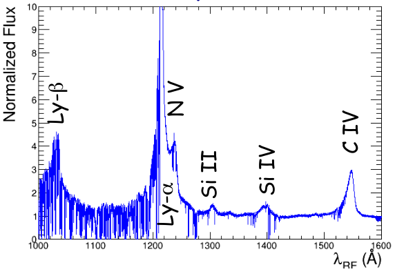
We define the Ly$\alpha$ forest by the range $1040<\lambda_{\rm RF}<1200\,$Å, thus $\sim 4000\,{\rm km\,s^{-1}}$ away from the quasar Ly$\beta$ and Ly$\alpha$ emission peaks to avoid contamination of the power spectrum by astrophysical effects in the vicinity of the quasar. The Ly$\alpha$ forest spans a redshift range $\Delta z\sim 0.65$ for a quasar at a redshift $z_{\rm qso}=4$. In order to improve the redshift resolution, we split the Ly$\alpha$ forest into three consecutive and non-overlapping sub-regions of equal length, hereafter called ‘$z$-sectors’. The splitting of each spectrum is done in such a way as to ensure that a ’$z$-sector’ lies on a single spectroscopic arm (either VIS or UVB), and to avoid the parts of the forest containing Damped Lyman Alpha (DLA) or Lyman limit (LLS) systems detected by Sánchez-Ramírez et al. (2016).

The largest possible mode is determined by the Nyquist-Shannon limit at $k_{\rm Nyquist}=\pi/\Delta v$. With a pixel size $\Delta v=c\Delta\lambda/\lambda=20\;{\rm km\,s^{-1}}$ and $11\;{\rm km\,s^{-1}}$ for the UVB and VIS arms, the largest mode is, respectively, $k_{\rm Nyquist}=0.16\;{\rm s\,km^{-1}}$ and $0.29\;{\rm s\,km^{-1}}$. We limit the analysis, however, to $k_{\rm max}=0.05-0.07\;{\rm s\,km^{-1}}$, depending on the absorption redshift, because of the large window function correction, at the largest $k$-modes, mostly due to the spectrograph resolution.

Sky lines affect the data quality by increasing the pixel noise. We identify major sky lines (such as lines at 5577, 5890, 6300, 6364, and $6864\,\AA$) and we replace the flux of each pixel impacted by a sky line by the average value of the flux over the rest of the forest. This procedure introduces a small $k$-dependent bias in the resulting power spectrum, which is negligible in this analysis due to the small number of sky lines in this wavelength region and the good spectrograph resolution.

The normalized transmitted flux fraction $\delta(\lambda)$ is estimated from the pixel flux $f(\lambda)$ by:

where $f_{\rm qso}^{1280}$ is a normalization equal to the mean flux in a $20\,$Å window centered on $\lambda_{RF}=1280\,$Å where $\lambda_{RF}=\lambda/(1+z_{\rm qso})$, $C_{q}(\lambda,z_{\rm qso})$ is the normalized unabsorbed flux (the mean quasar ‘continuum’) and $\overline{F}(z_{\rm Ly\alpha})$ is the mean transmitted flux fraction at the H i absorber redshift. Pixels affected by sky line emission are not included when computing the normalization. Since the mean quasar continuum is flat in the normalization region, the rejection of a few pixels does not bias the mean pixel value. The product $C_{q}(\lambda,z_{\rm qso})\overline{F}(z_{\rm Ly\alpha})$ is assumed to be universal for all quasars at redshift $z_{\rm qso}$ and is computed by stacking appropriately-normalized quasar spectra $f/f_{\rm qso}^{1280}$, thus averaging out the fluctuating Ly$\alpha$ absorption. The product $f_{\rm qso}^{1280}C_{q}(\lambda,z_{\rm qso})\overline{F}(z_{\rm Ly\alpha})$ represents the mean expected flux, and the transmitted flux fraction is given by $F=f/(f_{\rm qso}^{1280}C_{q})$. For a pixel at wavelength $\lambda$, the corresponding H i absorber redshift $z_{\rm Ly\alpha}$ can be inferred from $1+z_{\rm Ly\alpha}=\lambda/\lambda_{\rm Ly\alpha}$, where $\lambda_{\rm Ly\alpha}=1215.67$Å.

In the analysis of BOSS data Palanque-Delabrouille et al. (2013), we encountered two main issues: determination of noise power spectrum $P^{noise}(k)$ and correction of the spectrograph resolution. As the signal-to-noise ratio per pixel is much better in XQ-100 than in BOSS and since the data are at higher redshift, we can anticipate that with XQ-100 the impact of $P^{noise}(k)$ will be negligible. On the other hand, we want to study the small scales that are key for constraints on WDM. We aim at exploiting scales to $0.07\,{\rm s\,km^{-1}}$, three times smaller than with BOSS. As the spectral resolution of XSHOOTER is 3 to 5 times better than for BOSS, the knowledge and control of the spectrograph resolution is again a key issue of the analysis.

The spectral resolution of the UVB and VIS arms are derived from the slit widths, which were respectively $1.0^{\prime\prime}$ and $0.9^{\prime\prime}$. These slit widths provide a nominal resolving power of 4350 and 7450 as explained in López et al. (2016). However, for many observations, the seeing was smaller than the slit width, inducing an underestimate of the resolving power. To address this issue, we first determine the seeing with the raw spectra of XQ-100. The 2D spectra, as shown on Fig.2 (left plot), allow us to measure the seeing by fitting a Gaussian of the transversal distribution (i.e. orthogonal to the direction of the slit). We checked that the seeing thus measured is in good agreement with the seeing measured simultaneously at VLT (see Fig.2, right plot). On average the seeing is equal to $0.7^{\prime\prime}-0.8^{\prime\prime}$, better than the slit widths used during the observations.

As a consequence, we decided to compute our own determination of the spectral resolution, using the VLT seeing, namely (SEEING_MIN+SEEING_MAX)/2 from XQ-100_summary.fits file. We determine the resolution from the tables describing the XSHOOTER instrument (defined at XSH ()). When the seeing is smaller than the slit width, we substitute the slit width by the computed seeing, and compute the corresponding resolution.

To predict the Ly$\alpha$ flux power spectrum, we use the set of simulations extensively described in PY15 and BP16. The simulations are run using a parallel tree smoothed particle hydrodynamics (tree-SPH) code Gadget-3, an updated version of the public code Gadget-2 Springel et al. (2001); Springel (2005). The simulations are started at $z=30$, with initial transfer functions and power spectra computed with CAMB (Lewis et al., 2000), and initial particle displacements generated with second-order Lagrangian Perturbation Theory 2LPT¹¹ 1 http://cosmo.nyu.edu/roman/2LPT/. We include three particle types: collisionless dark matter, gas, and, when relevant, degenerate-mass neutrinos. We showed in Palanque-Delabrouille et al. (2015a) that considering inverted or normal neutrino mass hierarchy yields a flux power spectrum that differs by less than 0.05% from the degenerate-mass scenario, a level ten times lower than the statistical uncertainties in the simulation and almost two orders of magnitude below the data uncertainties. The degenerate-mass hypothesis is thus highly justified. The simulations cover the volume of a periodic 100 Mpc$/h$ box containing the equivalent of $3072^{3}$ particles of each type. Following a method originally suggested in McDonald (2003), we obtain this resolution by splicing together large-volume and high-resolution simulations, using a transition simulation that corrects the large box for its lack of coupling between small and large modes, and the high-resolution simulation for its small volume. We studied the accuracy of the splicing technique in Palanque-Delabrouille et al. (2015a) and we leave parameters free when fitting the data to account for residual biases.

The cosmological parameters are centered on the Planck 2013 best-fit values Planck Collaboration et al. (2013). Using simulations where one or two parameters at a time are given off-centered values, we compute first and second-order derivatives of the Ly$\alpha$ flux power spectrum with respect to each parameter, which we use to derive a second-order Taylor expansion of the predicted Ly$\alpha$ flux power spectrum. The cosmological parameters cover the range $H_{0}=67.5\pm 5~{\rm km\,s^{-1}\,Mpc^{-1}}$, $\Omega_{M}=0.31\pm 0.05$, $n_{s}=0.96\pm 0.05$, $\sigma_{8}=0.83\pm 0.05$. In all the runs, we keep $\Omega_{b}=0.0221$. While our central simulation assumes massless neutrinos, some runs include neutrinos with masses $\sum m_{\nu}=0.4$ or 0.8 eV. Where WDM is assumed, the dark matter particles are thermal relics with masses $m_{X}=2.5$ or 5.0 keV. All our simulation runs start at $z=30$, with initial conditions having the same random seed. Snapshots are produced at regular intervals in redshift from $z=4.6$ to 2.2, with $\Delta z=0.2$.

We test the influence of assumptions on the IGM astrophysics by running simulations for central and offset values of relevant parameters. The photo-ionization rate of each simulation is fixed by requiring the effective optical depth at each redshift to follow the empirical law $\tau_{\rm eff}(z)=A^{\tau}(1+z)^{\eta^{\tau}}$, with $A^{\tau}=0.0025\pm 0.0020$ and $\eta^{\tau}=3.7\pm 0.4$ in agreement with (Meiksin, 2009). This renormalization is done at the post-processing stage, as justified in Theuns (2005), allowing us to test the impact of different scalings without running new simulations. The IGM temperature-density relation $T=T_{0}\Delta^{\gamma-1}$ is obtained using simulations ran for $\gamma(z=3)=1.3\pm 0.3$ and $T_{0}(z=3)=14000\pm 7000\,$K. We use the quick-Ly$\alpha$ option to convert gas particles with overdensities exceeding $10^{3}$ and temperature below $10^{5}$ K into stars.

The analysis of the data is done with a frequentist approach. We showed in Palanque-Delabrouille et al. (2015b) that the constraints obtained with either a frequentist or a Bayesian (MCMC) approach were in excellent agreement. The large number of nuisance parameters that are now included in the fit, however, prevents the use of a Bayesian method where convergence is then hard to reach.

The parameters that are floated in the minimization procedure belong to three categories. The first category models a flat $\Lambda$CDM cosmology with free $H_{0}$, $\Omega_{M}$, $n_{s}$, $\sigma_{8}$ and either $\sum m_{\nu}$, $m_{X}$ or $m_{s}$. The second category describes the IGM, letting free the parameters described in table 1, namely $T_{0}$, $\gamma$, $\eta^{T_{0}}(z<3)$, $\eta^{T_{0}}(z>3)$, $\eta^{\gamma}$, $A^{\tau}$, $\eta^{\tau}$ and two amplitudes for the correlated absorption of Ly$\alpha$ with Si iii or Si ii. In particular, to take into account the redshift evolution of $T_{0}(z)$, $\gamma(z)$, we modeled them using a single power law for $\gamma$ and a broken power law at $z=3$ for $T_{0}$ as explained in Palanque-Delabrouille et al. (2015a).

Finally, the last category groups all nuisance parameters that allow us to account for uncertainties or corrections related to noise in the data, spectrograph resolution, modeling of the IGM, residual bias in the slicing technique, supernova and AGN feedbacks, and redshift of reionization. Details on the fit parameters and on the dependance with scale and redshift of the nuisance parameters can be found in Palanque-Delabrouille et al. (2015a).

The results for Ly$\alpha$ alone are shown in columns (1) to (3) of Tab. 3. Column (1) recalls the results of PY15 for BOSS Ly$\alpha$ alone. The maximization of the likelihood with Ly$\alpha$ data, imposing a Gaussian constraint $H_{0}=67.3\pm 1.0$, gives a best-fit value of the sum of the neutrino masses $\sum m_{\nu}$ equal to 0.41 eV and compatible with 0 at about $1\sigma$. The upper bound on $\sum m_{\nu}$ is thus $1.1$ eV (95% C.L.).

In column (2) of Tab. 3, we present the results with XQ-100 alone, using $P(k)$ measured with the method described in Sec. 2 . The upper bound on $\sum m_{\nu}$ is $1.2$ eV (95% C.L.), compatible with the upper bound from BOSS alone.

The other astrophysical and cosmological parameters are in very good agreement between BOSS-alone and XQ-100-alone. The largest differences observed are for $T_{0}$ and $\sigma_{8}$. They represent respectively $1.7\sigma$ and $1.4\sigma$. However, the comparison of BOSS and XQ-100 and the interpretation of differences in the best-fit parameters may be delicate as all the variables are correlated. In particular, we illustrate in Fig. 8 (left) the strong anti-correlation between $T_{0}$ and $\gamma$. As a result, a low value of $\gamma$ pushes $T_{0}$ to high values. In this neutrino-mass-oriented analysis, the likelihood is built in such a way as not to be too sensitive to underlying assumptions on IGM parameters, which we here treat as nuisance parameters. The shapes of $T_{0}(z)$ and $\gamma(z)$ are let free in the maximization of the likelihood as explained in Sec. 3.3.

Finally, by combining BOSS and XQ-100, see column (3), the best-fit value of $\sum m_{\nu}$ decreases to 0.34 eV and the upper bound on $\sum m_{\nu}$ tightens to $0.8$ eV (95% C.L.). The fitted values of astrophysical and nuisance parameters are all well within the expected range. The neutrino mass is correlated to $\sigma_{8}$ (-26%), $n_{s}$ (19%) and $\Omega_{m}$ (33%). Correlations between all other cosmological parameters have smaller amplitudes.

We now combine the Ly$\alpha$ likelihood (imposing no constraint on $H_{0}$) with the likelihood of Planck 2015 data that we derive from the central values and covariance matrices available in the official 2015 Planck repository. As in the previous section, we focus on the base $\Lambda$CDM$\nu$ cosmology. Column (4) of Tab. 3 shows the results for the combined set of Ly$\alpha$ (BOSS and XQ-100) and the base configuration we chose for Planck data, i.e. (TT+lowP) (cf. details in Sec. 3). In column (5), we extend the CMB measurements to (TT+TE+EE+lowP) and we add BAO data.

We illustrate in Fig. 8 (right) the main 2D contours on cosmological parameters. The small tension on $n_{s}$ between Ly$\alpha$ and Planck data, observed in Palanque-Delabrouille et al. (2015b); Palanque-Delabrouille et al. (2015a), is still present when including XQ-100 data, although its significance is reduced to 1.7 $\sigma$. We demonstrated in PY15, anyhow, that the tension on $n_{s}$ has little effect on the constraint on $\sum m_{\nu}$ because of the mild correlation between these two parameters (19% in Ly$\alpha$, -45% in Planck TT+lowP). As was already seen in PY15, $\sum m_{\nu}$ is mostly correlated to $\sigma_{8}$ (-26% in Ly$\alpha$, -95% in Planck TT+lowP) and to $\Omega_{m}$ (19% in Ly$\alpha$, 92% in Planck TT+lowP).

Fig. 9 shows that the combination of Planck and Ly$\alpha$ is a very efficient way of constraining cosmological parameters, especially $\sum m_{\nu}$. As we explained in PY15, Ly$\alpha$ data constrain $\Omega_{m}$ and $\sigma_{8}$ largely independently of $\sum m_{\nu}$ because they have different impacts on the shape of the power spectrum. On the other hand, in CMB data, $\sum m_{\nu}$ is strongly correlated with $\Omega_{m}$ and $\sigma_{8}$. For the Planck constraints, high $\sum m_{\nu}$ corresponds to low $\sigma_{8}$ because of the suppression of power on small scales by neutrino free streaming. The positive correlation between $\Omega_{m}$ and $\sum m_{\nu}$ is more subtle: with $\Omega_{c}h^{2}$ and $\Omega_{b}h^{2}$ well constrained by the acoustic peaks, raising $\sum m_{\nu}$ increases the matter density at low redshift after neutrinos become non-relativistic, and within $\Lambda$CDM this requires a decrease in $h$ to maintain the well determined angular diameter distance to last scattering, and this in turn corresponds to higher $\Omega_{m}$(see, e.g., §6.4 of Planck Collaboration et al. (2015)). The end result is that the Ly$\alpha$ and Planck contours intersect only near $\sum m_{\nu}=0$. By combining (BOSS and XQ-100) Ly$\alpha$ and Planck TT+lowP data, we constrain $\sum m_{\nu}$ to be less than 0.14 eV at 95% C.L.. Finally, adding polarization or BAO to the Planck + Ly$\alpha$ contours does not lead to significant further improvement of the constraints as shown in column (5) of Tab 3.

The current limit on $\sum m_{\nu}$ is a bit looser that the 0.12 eV bound of PY15, whereas we note a small improvement in the Ly-$\alpha$ alone constraint with the inclusion of XQ-100 (cf. Sec. 4.1). The origin of this result can be understood when plotting the $\chi^{2}$ profile for three combinations of data sets (cf. Fig. 10 (right)). The minimum for the BOSS Ly$\alpha$ + Planck configuration (red curve) occurs for $\sum m_{\nu}<0$. The fact that the CMB data sets have their minimum in the unphysical (negative $\sum m_{\nu}$) region was already discussed in Planck Collaboration et al. (2014). In the results presented in Tab. 3, the limit on the total neutrino mass is derived by computing the probability of $\Delta\chi^{2}(\sum m_{\nu})=\chi^{2}(\sum m_{\nu})-\chi^{2}(\sum m_{\nu}=0)$ with one degree of freedom. In the case of the (BOSS+XQ-100) Ly$\alpha$ + Planck configuration, the curvature of the $\chi^{2}$ profiles stays almost unchanged, but the position of the minimum is shifted closer to the physical ($\sum m_{\nu}>0$) region, causing a looser bound on $\sum m_{\nu}$.

The shift of the $\chi^{2}$ minimum into the physical region can be easily explained. By adding XQ-100, the combined value of $\sigma_{8}$ is smaller compared to BOSS alone (see first and second columns of Tab 3). The two parameters $\sigma_{8}$ and $\sum m_{\nu}$ are anti-correlated for Planck data as shown on Fig. 10 (left). As a consequence, XQ-100 pushes toward higher $\sum m_{\nu}$.

Finally, as shown in Fig. 10 (right) (blue curve), adding BAO data definitively forces the minimum back into the physical ($\sum m_{\nu}>0$) region. Hence, despite a much more constraining set of data (the limit at 3$\,\sigma$ or more is the tightest when all Ly$\alpha$, CMB and BAO data are included), we obtain a limit on the total neutrino mass of $\sum m_{\nu}<0.14$ eV at 95% CL, identical to the limit with Ly$\alpha$ and Planck.

To probe $\Lambda$WDM cosmology, we follow a similar approach as described in Sec.3.3. The only significant difference is related to the uncertainty on the reionization history of the universe. As the redshift at which the UV background onsets affects the Jeans smoothing scale of the baryon gas Gnedin and Hui (1998) in a manner similar to the free streaming scale of warm dark matter particles, altering the reionization redshift $z_{\star}$ impacts the definition of the WDM free streaming scale. Fig. 13 of McDonald et al. (2005) shows that an increase in the redshift of reionization from $z_{\star}=7$ to 17 suppresses the Ly$\alpha$ flux power spectrum in the largest $k$-modes present in the BOSS data ($k\sim 0.02\,\rm{s\,km^{-1}}$) by about 1% at $z=2.1$ and 4% at $z=4.0$. For XQ-100 where the power spectrum is measured at much smaller scales, ($k\sim 0.07\,\rm{s\,km^{-1}}$ at $z=4.0$), we are very sensitive to such an effect. Using the study of reionization by McDonald et al. (2005), we model the effect of reionization over the power spectrum and we introduce a nuisance parameter representing $z_{\star}$. This new parameter is let free in the likelihood with a constraint $z_{\star}=9.0\pm 1.5$. The central value and range of this external constraint are defined in order to encompass the most recent measurements of the redshift of reionization Hinshaw et al. (2013); Planck Collaboration et al. (2015); Planck Collaboration et al. (2016).

A fit to the power spectrum of XQ-100 Ly$\alpha$ forest, assuming the expansion rate value $H_{0}=67.3\pm 1.0\;\rm{km~s^{-1}~Mpc^{-1}}$ issued by Planck Collaboration et al. (2015), yields a lower bound $m_{X}>2.08\,\rm{keV}$ (95% C.L.) for thermal relics and $m_{s}>10.2\>\rm{keV}$ for Dodelson-Widrow Dodelson and Widrow (1994) sterile neutrinos (95% CL). These bounds are roughly twice lower than the bounds given with BOSS alone by BP15 in Fig. 11 (left) and Tab. 4.

When combining XQ-100 with BOSS Ly$\alpha$ forest power spectra, the 95% C.L. limit is slightly improved compared to the one from BOSS alone. It increases from $m_{X}\gtrsim 4.09\>\rm{keV}$ to $m_{X}\gtrsim 4.17\>\rm{keV}$. The $3~\sigma$ bound shows a more significantly improvement, increasing from $m_{X}\gtrsim 2.74\>\rm{keV}$ for BOSS alone to $m_{X}\gtrsim 3.10\>\rm{keV}$ for the combined BOSS+XQ-100 data set.

The reason of this improvement is clearly illustrated in Fig. 11 (right), which shows the $\chi^{2}$ profile for two combinations of data sets: BOSS alone and BOSS+XQ-100. Clearly, the curvature increases by adding XQ-100 but the position of the minimum is shifted into the physical ($1/m_{x}>0$) region, explaining a small improvement of the 95% C.L bound and a larger improvement at higher significance ($3~\sigma$ or more). Fitting the $\chi^{2}$ profile by $\Delta\chi^{2}(1/m_{X})=\chi^{2}_{0}+(1/m_{x}-1/m_{x_{0}})^{2}/\sigma^{2}+\alpha\cdot(1/m_{x}-1/m_{x_{0}})^{4}$, the parameter $\sigma$ provides an estimator of the statistical sensitivity on $1/m_{X}$. The combination with XQ-100 allows us to reduce $\sigma$ from 0.15 to 0.12, representing a 25% gain in statistical sensitivity.

Although we believe that a Gaussian constraint with a sigma of 1.5 on $z_{\star}$ allows us to encompass the range of allowed $z_{\star}$ from CMB results (in particular Hinshaw et al. (2013); Planck Collaboration et al. (2015); Planck Collaboration et al. (2016)), we released the constraint on $z_{\star}$, allowing for a wider variation range, to study the impact on the warm dark matter mass bound. The effect is small: If we increase the sigma to 2.5, the 95% CL limit on $m_{X}$ decreases from $4.17\>\rm{keV}$ to $3.90\>\rm{keV}$.

Finally, it has been recently argued in Garzilli et al. (2015) that the small-scale cutoff in the power spectrum can be accounted for by a warm IGM rather than a warm DM particle. By adding XQ-100 to BOSS data, in Fig 12, we do not observe any significant change in the IGM temperature $T_{0}$ nor in the logarithmic slope $\gamma$ of the dependence of the IGM temperature with overdensity $\delta$. Additional Ly$\alpha$ forest data at higher redshifts ($z\geq 4.5$) are needed to better study this hypothesis.

In summary, with the inclusion of XQ-100 in addition to BOSS into the analysis of BP16, we confirm our original limit from BOSS alone, in the case of $\Lambda$WDM model. We issue tighter bounds on pure dark matter particles: $m_{X}\gtrsim 4.17\>\rm{keV}$ (95% C.L.) for early decoupled thermal relics and its corresponding bound for a non-resonantly produced right-handed neutrino $m_{s}\gtrsim 25.0\>\rm{keV}$ (95% C.L.).

Recently, the XQ-100 team released the measurement of the Ly$\alpha$ forest power spectrum in Iršič et al. (2016). Applying the methodology of BP16 to their XQ-100 power spectrum alone, we find a bound at $m_{X}>1.90\>\rm{keV}$ (95% C.L.) for thermal relics, which is fully compatible with our bound, $m_{X}>2.08\>\rm{keV}$ (95% C.L.). We suspect that the slightly tighter limit we obtain comes from the better estimation of the resolution as explained in Sec. 2.3. By removing the highest $k$-bins, we indeed observe a small trend that may explain partially the difference. For instance, when we do not take into account the $k$-bins between 0.06 and $0.07\>{\rm(km/s)}^{-1}$ for the highest redshift bin, the limit decreases from 2.08 to $2.03\>\rm{keV}$. Tab. 4 and Fig. 13 summarize the comparison on the 95% confidence limits obtained with the two power spectra.

The analysis presented in Iršič et al. (2017) shows that the combination of the XQ-100 and HIRES/MIKE datasets can significantly improve the limit on $m_{X}$. Indeed, the two datasets have different degeneracies between astrophysical and cosmological parameters that are disentangled when the data are combined, thanks to the higher resolution of the HIRES/MIKE spectrograph. By studying the three datasets BOSS, XQ-100 and HIRES/MIKE, we can thus expect an improvement over BOSS+XQ-100. However, as noted before, since the first snapshot of our simulations is taken at $z=4.6$, we can only use the lowest two redshift bins of HIRES/MIKE ($z=4.2$ and $z=4.6$) .

Fig. 14 (left) illustrates the improvement in the $1/m_{X}-\Omega_{m}$ plane. The new bounds with HIRES/MIKE are $m_{X}\gtrsim 4.65\>\rm{keV}$ and $m_{s}\gtrsim 28.8\>\rm{keV}$ (95% C.L.). As we explained in Sec. 5.1, the fit of the $\chi^{2}$ profile shown on Fig. 14 (right) by a quadratic term demonstrates a reduction of $\sigma$ from 0.123 to 0.105 and finally 0.093 when we add successively the $z=4.2$ and $z=4.6$ redshift bins of HIRES/MIKE. It represents a gain of respectively 17% and 13% in statistical sensitivity. In total, it is a gain in statistical sensitivity of 60% with respect to BOSS alone. We do not observe such an impressive gain for the 95% CL bound because the $\chi^{2}$ minimum moves from the negative (unphysical) region to the physical region. Our final limit on $m_{X}$ is in perfect agreement with the new bound $m_{X}\gtrsim 5.3\>\rm{keV}$ given in Iršič et al. (2017), confirming the consistent bounds measured by the various teams Seljak et al. (2006b); Viel et al. (2013); Baur et al. (2016); Iršič et al. (2017).