Structure and variability in the corona of the ultrafast rotator LO Peg
Abstract
Context. Low-mass ultrafast rotators show the typical signatures of magnetic activity and are known to produce flares, probably as a result of magnetic reconnection. As a consequence, the coronae of these stars exhibit very large X-ray luminosities and high plasma temperatures, as well as a pronounced inverse FIP effect.
Aims. To probe the relationship between the coronal properties with spectral type of ultra-fast rotators with P, we analyse the K3 rapid-rotator LO Peg in comparison with other low-mass rapid rotators of spectral types G9-M1.
Methods. We report the results of a ks long XMM-Newton observation of LO Peg and investigate the temporal evolution of coronal properties like the temperatures, emission measures, abundances, densities and the morphology of the involved coronal structures. In addition, we also use the XMM-Newton data from a sample of rapid rotators and compare their coronal properties to those of LO Peg.
Results. We find two distinguishable levels of activity in the XMM-Newton observation of LO Peg, which shows significant X-ray variability both in phase and amplitude, implying the presence of an evolving active region on the surface. The X-ray flux varies by , possibly due to rotational modulation. During our observation a large X-ray flare with a peak X-ray luminosity of erg/s and a total soft X-ray energy release of 7.3 erg was observed. Further, at the onset of the flare we obtain clear signatures for the occurrence of the Neupert effect. During the flare a significant emission measure increase in the hotter plasma component is observed, while the emission measure in the cooler plasma component is only marginally affected, indicating that different coronal structures are involved. The flare plasma also shows an enhancement of iron by a factor of 2 during the rise and peak phase of the flare. The electron densities measured using the O vii and Ne ix triplets during the quiescent and flaring state are 6 cm-3 and 9 cm-3, respectively, and the large errors prevent us from finding significant density differences between quiescent and flaring states. Our modeling analysis suggests that the scale size of the flaring X-ray plasma is smaller than 0.5 R⋆. Further, the flare loop length appears to be smaller than the pressure scale height of the flaring plasma. Our studies show that the X-ray properties of the LO Peg are very similar to those of other low-mass ultrafast rotators, i.e., the X-ray luminosity is very close to saturation, its coronal abundances follow a trend of increasing abundance with increasing first ionisation potential, the so-called inverse FIP effect.
Conclusions.
Key Words.
X-rays: stars–stars: coronae–stars: atmosphere – stars: flare –stars: low-mass – stars: individual: LO Peg1 Introduction
The Sun is usually considered as a prototype of a low mass star and we often extrapolate our knowledge of the properties of the Sun to interpret observations of other stars. Given that our Sun, a middle-aged main-sequence star, has an X-ray emitting corona, the question arises whether the solar corona serves as a good proxy also for other stars. Indeed, solar-like stars as a class have been found to be X-rays emitters with X-ray luminosities in the range of 1026-31 erg/s (Rosner et al., 1985). Furthermore, a few low mass stars are considerably more X-ray luminous than the Sun, and these so-called active low-mass stars are very often also rapid rotators (Pallavicini et al., 1981) with saturated coronae, i.e., the X-ray luminosities of these stars scale with their bolometric luminosities such that . As a result, the X-ray luminosities of active stars of spectral type K and M type range from 1028 to 1030 erg/s (Rosner et al., 1985), raising the question in what respect the coronae of these stars differ from the solar corona and how they accommodate the observed excess X-ray emission. The X-ray emission from a stellar corona is believed to come from an optically thin plasma and therefore scales with the (volume) emission measure , where denotes density and the coronal volume. Stars with larger X-ray luminosities than the Sun therefore must have coronae with a larger volume or a larger coronal density or possibly both.
Active stars also possess magnetic fields which manifest themselves in observable features like star spots, flares, emissions in activity-sensitive lines like those from Ca II H&K, H, etc., large luminosities in the X-ray and EUV regime and, last but not least, activity cycles (Pizzolato et al., 2003). Two well-known examples of such extremely active, ultra-fast rotators are BO Mic and AB Dor, both of which have been previously studied at X-ray wavelengths in great detail (cf., Wolter et al. 2008; Lalitha et al. 2013) and both of which show moderate flares at X-ray and/or UV wavelengths in nearly every stellar rotation and occasionally they produce very large flares.
Just like BO Mic and AB Dor, the star LO Peg (BD +22 4409) is also a very young low mass rapid rotator with a spectral type between K3 and K8 (Jeffries et al., 1994; Pandey et al., 2005). LO Peg is located at a distance of 24 pc and thought to be a member of the local association (Jeffries & Jewell, 1993a; Montes et al., 2001). On the basis of its galactic space motion and its large fractional EUV-Luminosity of -3.53, Jeffries & Jewell (1993b) identify LO Peg as a member of the Pleiades moving group with an age between 20 - 150 Myr, while Zuckerman & Song (2004) identify LO Peg as a member of AB Dor group of 50 Myr old stars in the solar neighbourhood. Jeffries et al. (1994) suggest a rotation period of LO Peg between 0.3841-0.42375 day from V-band photometry. The same authors also find an equatorial rotational velocity 691 km/s.
LO Peg was detected as a X-ray source in the ROSAT all-sky survey (RASS) as the source 1RXS J213101.3+232009 (Voges et al., 1999) with an X-ray luminosity (in the 0.1 - 2.0 keV energy band) of 5.1 1029 and a ratio of X-ray to bolometric luminosity of . LO Peg was also detected with the ROSAT Wide Field camera (WFC) as the source RE 2131 +23.3 and with the Extreme Ultra-Violet Explorer (EUVE) as the source EUVE 2131+233 (Malina et al., 1994); the coarse X-ray spectral properties of LO Peg were explored with a short ROSAT PSPC observation by Pandey et al. (2005). All the available data suggest that LO Peg does indeed have a powerful corona close to the saturation limit indicating that the star is magnetically very active.
The magnetic activity of LO Peg was also demonstrated by its strong H and Ca ii H&K emission lines (Jeffries et al., 1994). Furthermore, Eibe et al. (1999) presented evidence for optical flaring on LO Peg and an intense down-flow of material. The rapidly changing surface activity and high equatorial rotational velocity make LO Peg an interesting object in terms of stellar activity and its relation to stellar rotation. Since the discovery of LO Peg as a variable star, it has been the subject of detailed studies like spectral surface mapping and long-term photometric observations. For example, Taš (2011) showed that LO Peg has an active longitude of lifetime 1.3 years and 4.8 yrs activity cycle period.
In order to provide a more detailed picture of the coronal properties of this ultra-fast rotator, we have obtained XMM-Newton data covering a full rotation period of LO Peg, which we present and discuss in this paper. Our paper is structured as follows: In Section 2 we describe our observations obtained with XMM-Newton. In Section 3 and 4, we characterise the temporal and spectral behaviour of LO Peg. The coronal properties of LO Peg are compared with other rapid rotators in Section 5 and in Section 6 we present our summary and conclusions.
2 Observations and data analysis
The new X-ray data on LO Peg presented in this paper have been obtained with the XMM-Newton satellite on November, 30th 2014 (PI Lalitha S.; Obs ID: 0740590101). Onboard the XMM-Newton satellite there are three co-aligned X-ray telescopes (Jansen et al., 2001) and the European Photon Imaging Camera (EPIC; see Strüder et al. 2001; Turner et al. 2001), which contains three CCD cameras (one pn and two MOS cameras) with a sensitivity range in the energy band 0.2 - 15 keV. The EPIC X-ray CCD detectors provide medium-resolution imaging spectroscopy E/E 20 - 50 and temporal resolution at the sub-second level. The X-ray telescopes with the MOS detectors are also equipped with simultaneously operated reflection gratings (the so-called Reflection Grating Spectrometer – RGS; den Herder et al. 2001), which provide high-resolution X-ray spectroscopy in the energy range 0.35 - 2.5 keV. Finally, XMM-Newton carries an Optical Monitor (OM), i.e., an optical/UV telescope with different filters for imaging and time-resolved photometry (Mason et al., 2001).

Our XMM-Newton observations have a total duration of 42 ks, covering more than one rotation period of LO Peg (P 36 ks). Useful data for LO Peg are available from the OM, EPIC, and the RGS detectors. The pn and MOS detectors were operated with the medium filter in imaging and small window mode, while the OM was operated in fast mode with a 0.5 sec cadence using the UVM2 band filter covering a band pass between 205 - 245 nm.
All X-ray data were reduced with the XMM-Newton Science Analysis System (SAS) 11 1 The XMM-Newton SAS user guide can be found at http://www.cosmos.esa.int/web/xmm-newton/documentation/ software, version 13.0. EPIC light curves and spectra were obtained using standard filtering criteria, spectral analysis was done with XSPEC version 12.8.1. (Arnaud, 1996) for the overall fitting processes. For model fitting we always assume a collisionally ionised optically thin gas as calculated with the Astrophysical Plasma Emission Code (APEC) 22 2 http://hea-www.harvard.edu/APEC/; Smith et al. 2001) and abundances are calculated relative to the solar photospheric values of Grevesse & Sauval (1998).

3 Results
3.1 Timing analysis of XMM-Newton data: Overview
For an overview of our XMM-Newton data we plot in Fig. 1 the light curves simultaneously recorded with the OM (top panel) and the EPIC-pn (middle panel) detectors, each binned to 100 s; the arrows in the plot show different time bins used for our later spectral analysis. As is evident from Fig. 1, a large flare occurred towards the end of observation when the count rate increased from quiescent values of 4 cts to 17 cts in the pn detector and from 1 cts to 5 cts in the MOS detectors.
To give a coarse description of the changes in the spectral behaviour of the X-ray emission we compute a hardness ratio (HR) for the pn as the ratio of the number of counts in hard band (2.0-10.0 keV) and the soft band (0.2-1.0 keV), which is plotted in the lower panel of Fig. 1. We note that the HR values seem to be more or less constant at a level of without significant variation during the quiescent phase, while a clear hardening to is seen during the large flare.
3.1.1 Rotational modulation ?
In addition to the flare observed toward the end of our observations, LO Peg also shows some modulations in the overall light curve. In Fig. 2 we plot the pn light curves folded with the ephemeris by Dal & Tas (2003) HJD 2,448,869.93 + 0.42375 E; we show our data twice, first in the original form and then shifted by exactly one rotational period. As shown in Fig. 2, our observations cover hardly more than one rotation period and the large flare occurred at the very end so that no real phase overlap between adjacent orbits is available in our data. Yet it appears that at the end of the orbit the count rate level is approximately the same as at the beginning and it is tempting to interpret the apparent light curve modulation as a rotation-induced modulation. The light curve reaches its maximum at phase 0.25-0.3, and the large flare took place between phases 1 - 1.1, consistent with the interpretation that a more active hemisphere could have been in view.
Assuming that the quiescent emission of LO Peg exhibits partial rotational modulation, we can estimate the degree of modulation using the amplitude of a simple sine wave fit to the data. Using only the quiescent data, we find an amplitude of 0.45 0.01 cts and a mean level of 3.39 0.17 cts , corresponding to a rotational modulation of 14.

3.1.2 Neupert effect

In Fig. 3 we show a close-up view of the LO Peg flare light curve in various bands, i.e., in the “soft” X-ray band (between 0.2-2 keV; orange), in the “hard” X-ray band (between 2-10 keV; cyan) and in the total X-ray band (between 0.2-10 keV; violet). We furthermore plot the time derivative of soft X-ray EPIC light curve (black) as well as the OM light curve (red), all the lightcurves are binned to 100 s and shifted to be around zero and scaled in amplitude to be as consistent as possible with the time derivative “light” curve. A visual inspection of Fig. 3 clearly indicates the peak of the harder X-ray band (cyan curve) precedes the peak of the softer X-ray band (orange curve) by 800-1000s, while the OM light curve peak (red) precedes the peak of the harder X-ray band (cyan curve) by about 15 minutes or 900 s; the shape of the time derivative of the soft X-ray EPIC light curve (black) agrees well, albeit not perfectly, with the OM light curve, with a peak delay of 2 bins or 400 s. This phenomenology suggests to interpret the OM emission as a proxy for the expected non-thermal radiation as a result of electron impingement on the chromosphere of LO Peg, which leads to the observed (thermal) X-ray flare, and thus as evidence for the Neupert effect.
We investigated further evidence for the Neupert effect during the rise phase of the flare. If, during a flare, the energy contained in all the accelerated particles is used for chromospheric and coronal heating, the time integral of the emission due to the accelerated particles or one of its proxies like hard X-ray emission, white-light emission, etc. resembles the rise of the flare light curve in the soft X-ray band (Neupert, 1968). This can be represented as
where FSXR and FHXR represent the soft and hard (non-thermal) X-ray fluxes, respectively.
Since there is no HXR data for our observations we use the OM data as a proxy for the emission due to the accelerated particles. In Fig. 3, we also plot the time derivative of soft X-ray EPIC light curve in black along with the ultra-violet band (optical monitor in pink). We note that the EPIC light curve during flare rise matches the shape of the OM light curve.
Cross-correlating the OM light curve and the time derivative of the X-ray light curves, we obtain a time-lag between the two peaks to be 250s, using the Z-transformed Discrete Correlation Function (ZDCF) technique described by Alexander (1997), much less than the delay between the soft X-ray and OM peak. This strongly suggests that indeed the optical/UV peak is a good proxy of the emission due to accelerated particles, preceding the bulk of the soft X-ray emission.
3.2 Spectral analysis of XMM-Newton data: Overview
Next, we examine the EPIC and RGS spectra of LO Peg extracted during flaring and quiescent intervals to study plasma temperatures, emission measures and abundances change as a result of flaring. In Fig.4, we plot the quiescent time averaged 1st order RGS 1 (black data points) and RGS 2 (red points) in the 10-26 wavelength range. The strongest lines are identified and labelled and are – as expected – due to oxygen, neon, iron and nitrogen.
During the course of a flare, fresh material from the chromosphere is heated, evaporated and transported into the corona, thus temporarily changing the coronal emission measure and possibly the coronal abundances. In Fig. 5, we plot the EPIC pn spectra extracted during quiescence (in black) and the flare (in red). The flare-related changes in the spectral energy distribution are very much evident; the spectral hardening is already apparent in the lower panel of Fig. 1 depicting the hardness ratios.
Along with the flare related changes, we also examine possible orbital variations by dividing the overall quiescent spectra in periods dubbed as “Quiet 1” and “Quiet 2” (the time bins for the spectra are as shown in Fig. 1) and model the pn, MOS and RGS X-ray spectra. We specifically determine the temperatures, emission measures and abundances relative to solar values (Grevesse & Sauval, 1998) with simultaneous iterative global XSPEC fits to the combination of EPIC and RGS (RGS+PN or RGS+MOS) spectra with variable-APEC (VAPEC; Smith et al. 2001) plasma models. As is often observed (Güdel et al., 2001; Robrade & Schmitt, 2005; Lalitha et al., 2013), we require multi-temperature components to achieve an adequate description of the observed coronal spectra. We use combinations of two, three and four temperature components and find that a three temperature component model leads to an adequate description of the data. We fit each of these spectra in the full 0.2 - 10 keV energy range. For fitting the RGS spectra, the temperature and the abundances of elements like carbon, nitrogen, oxygen, neon and iron are allowed to vary freely and independently, however, the abundances are fixed among the different APEC temperature components. For fitting EPIC-MOS or pn spectra we allow the magnesium, sulphur, and silicon abundances to vary along with the oxygen, neon and iron abundance. However, the carbon and nitrogen abundances are fixed to values obtained from the RGS, which is more sensitive to strong individual lines of these elements. In Tab. 1, we summarise the results of this fitting procedure along with the 90% confidence range errors. Tab. 1 shows that the quiescent state is characterised by dominant plasma components at , and MK, while during the flare the coronal temperature bins increase to , and MK. During the flare, a pronounced enhancement of the emission measure at keV is present, indicating the rise of emission measure at a higher temperature. The quiescent bins (quiet 1 and quiet 2) does not show any significant difference in the coronal properties when compared to the overall quiescent time-bin; suggesting no changes in coronal properties with orbital variation.

| Param | Quiet | Quiet1 | Quiet2 | Flare | ||||
|---|---|---|---|---|---|---|---|---|
| RGS+PN | RGS+MOS | RGS+PN | RGS+MOS | RGS+PN | RGS+MOS | RGS+PN | RGS+MOS | |
| kt1 [keV] | 0.26 | 0.27 | 0.26 | 0.27 | 0.26 | 0.26 | 0.30 | 0.32 |
| EM1 [1052 cm-3] | 1.16 | 0.94 | 1.14 | 1.06 | 1.15 | 0.93 | 2.24 | 1.21 |
| kt2 [keV] | 0.65 | 0.66 | 0.64 | 0.66 | 0.66 | 0.66 | 1.00 | 1.00 |
| EM2 [1052 cm-3] | 1.99 | 1.70 | 2.62 | 1.86 | 1.73 | 1.64 | 2.90 | 1.82 |
| kt3 [keV] | 1.66 | 1.56 | 1.81 | 1.58 | 1.62 | 1.52 | 2.87 | 2.81 |
| EM3 [1052 cm-3] | 1.29 | 1.43 | 1.58 | 2.00 | 1.00 | 1.08 | 7.73 | 7.85 |
| C | 0.60 | 0.51 | 0.78 | 0.16 | 0.45 | 0.31 | 0.89 | 1.13 |
| N | 0.53 | 0.65 | 0.66 | 0.76 | 0.48 | 0.55 | 0.54 | 1.64 |
| O | 0.38 | 0.46 | 0.39 | 0.47 | 0.36 | 0.41 | 0.41 | 0.74 |
| Ne | 1.17 | 1.37 | 1.19 | 1.38 | 1.14 | 1.28 | 0.81 | 1.24 |
| Mg | 0.26 | 0.31 | 0.21 | 0.30 | 0.29 | 0.33 | 0.11 | 0.31 |
| Si | 0.36 | 0.28 | 0.37 | 0.27 | 0.33 | 0.26 | 0.44 | 0.46 |
| S | 0.23 | 0.31 | 0.24 | 0.32 | 0.25 | 0.33 | 0.12 | 0.25 |
| Fe | 0.20 | 0.23 | 0.18 | 0.23 | 0.22 | 0.23 | 0.34 | 0.50 |
| 1.23 | 1.22 | 1.14 | 1.04 | 1.23 | 1.22 | 1.01 | 0.97 | |
| DOF | 1273 | 1136 | 704 | 585 | 735 | 615 | 704 | 571 |
| LX [erg/s] | 29.69 | 29.68 | 29.77 | 29.76 | 29.62 | 29.62 | 30.21 | 30.20 |
Note: the errors are estimated with 90% confidence limit. LX indicates the 0.2-10 keV luminosity.


The abundance patterns of LO Peg during different activity states are shown in Fig. 6, where we plot the abundances with respect to solar photospheric abundances against the FIP (First Ionisation Potential) of the corresponding element. The top and bottom panels show the abundance patterns obtained for RGS+PN and RGS+MOS combinations, respectively, for the quiescent and the flaring time bins. Inactive stars like the Sun show the FIP effect, where elements with low-FIP elements like Fe, Si, and Mg are enhanced in the corona when compared to high-FIP elements like C, N, O, and Ne. A reversed pattern, the inverse FIP effect with enhanced high-FIP elements when compared to the low-FIP elements, is frequently observed in active stars (e.g., Brinkman et al. 2001, Audard et al. 2003). The abundance pattern of LO Peg indicates an inverse FIP effect as can be seen in Fig. 6. Furthermore, during the flare some of the abundances such as Fe, O, and Si, are found to be slightly higher (albeit with uncomfortably large errors), and the Fe and Si abundances also rise compared to the high-FIP elements. In Figure7, we plot the evolution of Fe abundance showing a significant increase from the quiescence level before the flare to a maximum during flare peak and then decreases to the pre-flare values. All this is consistent with the picture that the fresh chromospheric material evaporates into the corona, thus changing the elemental abundances. We note that the global fit to the data using APEC models actually measures the absolute abundance constrained by the flux in the line (which is proportional to the abundance of the element producing the line) and the overall fit to the continuum, which is dominated by the hydrogen and helium content of the plasma as the main donors of electrons.

3.2.1 Emission measure distribution
In contrast to the abundances, emission measures and temperatures of the coronal plasma change more significantly during the flare evolution. The plasma emission measure increases and the spectra hardens as the temperatures rise (see Fig. 5 ). For instance, the Fe line complex at 6.7 keV, which is formed at 40 MK, appears only during the flaring state.
We carry out a quantitative study of the temporal evolution of the plasma temperature during different activity states by constructing the emission measure distribution (EMD). We use the pn, MOS and RGS data to study the changes in the EMD during different activity states. To construct an EMD we use a 6-T VAPEC model with a fixed temperature grid (put at energies of 0.2, 0.3, 0.6, 1.2, 2.4, 4.8 keV), where the first two components represent cool plasma (2-5 MK), the third and fourth temperature components represent medium temperature plasma (5-20 MK) and the last two components represent the hot plasma (20-60 MK). The abundances of neon, magnesium, oxygen, silicon, sulphur and iron are allowed to vary freely and independently, but are constrained to be same among all the other VAPEC temperature components. A graphical representation of the results on the EMDs using pn (in black), MOS (in red) and RGS (in blue) data for LO Peg during different activity states is shown in Fig. 8. During the quiescent state the EM peaks around 7 MK and the hot component is only marginally detected. However, during the flare we note a peak at 3.5 MK and a large amount of additional plasma at around 30 MK with the EM rising by a factor of 7 at 30 MK. There is little or no change in the cool plasma and the main influence due to the flare is the increased amount of high temperature emission measure.


3.2.2 Coronal densities
Using the XMM-Newton RGS spectra we investigate the electron densities of coronal plasma from the density-sensitive line ratios of forbidden to inter-combination lines of the helium-like triplets of O vii, the theory of which has been described in detail by Gabriel & Jordan (1969). If the electron collision rate is sufficiently high, the ions in the upper level of the forbidden transition level do not return to the ground level radiatively, instead, the ions are collisionally moved to the upper level of the inter-combination transitions, from where they eventually decay radiatively to the ground state. Therefore, the resulting ratio of the forbidden to inter-combination line (f/i) are sensitive to density.
| ion | line | Quiet | Quiet1 | Quiet2 | Flare |
|---|---|---|---|---|---|
| resonance (r, 21.60 Å) | 23.607.71 | 7.263.83 | 15.234.99 | 8.274.00 | |
| inter-combination (i, 21.80 Å) | 24.527.86 | 5.872.57 | 17.507.38 | 3.692.10 | |
| O vii | forbidden (f, 22.10 Å) | 25.245.99 | 9.074.13 | 18.5310.20 | 5.892.57 |
| r | 1.070.42 | 1.540.97 | 1.050.73 | 1.591.14 | |
| log(ne) [cm-3] | 10.810.76 | 10.720.55 | 10.810.57 | 10.710.50 | |
| resonance (r, 13.44 Å) | 76.9818.45 | 34.268.59 | 46.679.45 | 19.425.49 | |
| inter-combination (i, 13.55 Å) | 45.9722.32 | 12.376.42 | 25.827.88 | 3.401.83 | |
| Ne ix | forbidden (f, 13.69 Å) | 56.3723.23 | 26.118.05 | 30.859.78 | 8.223.99 |
| r | 1.220.78 | 2.111.27 | 1.190.52 | 2.411.75 | |
| log(ne) [cm-3] | 11.960.11 | 11.820.12 | 11.970.08 | 11.780.15 |


The He-like triplet of Ne ix and O vii are strong enough in our observations to be used to obtain characteristic electron densities in the source region. The f, i and r lines for He-like triplets of Ne and O are fitted using Gaussian profiles to each of the line components. In Fig. 9, we show the He-like triplets of Ne and O during the quiescent state. The measured line counts, calculated ratios and electron densities are listed in Tab. 2); note that the quoted O vii line counts are mean counts obtained from both the RGS1 and RGS2, while the Ne ix triplet is recorded only by the RGS2. To convert the measured f /i ratios to densities, we use the expression
where is the low-density limit and is the so-called critical density. We adopt the values from Pradhan & Shull (1981) and use = 3.95 and = 3.1 1010 cm-3 for O vii and = 3.5 and = 5.9 1011 cm-3 for Ne ix. The formal electron density calculated for LO Peg using O vii during quiescence and flare are log ne[cm-3]10.810.76 and 10.710.50, respectively, while we find log ne[cm-3]11.960.11 and 11.780.15, during quiescent and flaring states for Ne ix. Unfortunately, the number of measured counts in the f and i lines are rather small, leading to large errors. While we can state that the Ne ix emission is likely from a high density plasma region, we detect no significant differences between the quiescent and flaring plasma, yet the errors are so large that we cannot exclude an (expected) density increase in the flaring plasma. Finally, we note that the oxygen and neon triplet probe only temperatures between 1-4 MK and therefore the lines do not represent the major high-temperature component of the flare.
4 Discussion
4.1 Comparison with similar stars
We now compare the derived coronal properties of LO Peg with the properties of other ultra-fast rotators, i.e., AB Dor, BO Mic, PZ Tel, HK Aqr and YY Gem.
-
a) AB Dor is a well-studied example of an extremely active ultra-fast rotator (Prot = 0.51 d, d 15 pc, Guirado et al. 2011), which shows signatures of activity at all wavelengths. In particular, AB Dor shows strong photometric variability due to spots on its surface and is very bright in X-rays (LX 11030 erg/s, Lalitha et al. 2013).
-
b) BO Mic is an highly active young K-dwarf similar to AB Dor. BO Mic is also an ultra-fast rotator with a rotation period Prot = 0.38 d). Its typical quiescent X-ray luminosity of is 9 1029 erg/s. Several flares are observed on BO Mic, where the flare energy can increase by up to two orders of magnitude (Kurster, 1995).
-
c) PZ Tel is classified as a single K0V star with a rotation period of 0.94 d located at a distance 49 pc (Coates et al., 1980; Innis et al., 1984; Perryman et al., 1997; Zuckerman & Webb, 2000). PZ Tel is a young post T-Tauri star (20 Myr, Favata et al. 1998) with an X-ray luminosity of 2.81030 erg/s (Stelzer & Neuhäuser, 2000).
-
d) HK Aqr is one of the fastest rotating M-dwarfs with a rotation period of 0.43 d ( sin = 69 km s-1, Young et al. 1990), located at a distance of 22 pc. HK Aqr is a single star with a quiescent X-ray luminosity of 2 1029 erg/s.
-
e) YY Gem (Castor C) is the faintest member of a triple system (Castor A+B+C) with an X-ray luminosity of 2 - 8 1029 erg/s, located at a distance of 15 pc. YY Gem itself is a spectroscopic binary, in fact it is the brightest known eclipsing binary of the type dMe. Both components are in a circular and synchronous orbit with an inclination angle of (Pettersen, 1976) and a period of 0.81 d (Kron, 1952), both components have have almost the same spectral type. The YY Gem system is again magnetically very active star with a high flare rate, dark cool star-spots from spectroscopic and photometric observations and X-ray variability (see Güdel et al. 2001; Hussain et al. 2012, and references therein).
We list the physical properties of our comparison stars along with those of LO Peg in Tab. 3.
| Star | Type | Dist | V | Age | v | Prot | log LX | |
|---|---|---|---|---|---|---|---|---|
| pc | mag | Myr | km/s | days | erg/s | |||
| AB Dor | K1 V | 15 | 6.99 | 50 | 90 | 0.51 | 29.93 | -3.25 |
| BO Mic | K0 V | 44 | 9.33 | 30 | 132 | 0.38 | 29.94 | -3.07 |
| HK Aqr | M0 Ve | 22 | 10.87 | 200 | 70 | 0.44 | 29.24 | -3.18 |
| YY Gem | M1 | 15 | 9.83 | 350 | 37 ? | 0.81 | 29.39 | -2.95 |
| PZ Tel | G9 IV | 50 | 8.34 | 20 | 70 | 0.94 | 30.34 | -3.20 |
| LO Peg | K3 V | 25 | 9.25 | 30 | 70 | 0.41 | 29.70 | -3.11 |
XMM-Newton observations of YY Gem are described by Stelzer et al. (2002), and those of BO Mic by Wolter et al. (2008), and those of AB Dor by Lalitha et al. (2013), while there appear to be no publications of the XMM-Newton observations of PZ Tel and HK Aqr. To avoid any biases in the estimated coronal properties we carry out a detailed analysis of all these stars similar to our analysis of LO Peg and obtain their coronal properties such as emission measures, abundances, and coronal temperatures using our global fitting approach.
We simultaneously fit the medium-resolution EPIC data and high-resolution RGS data of each of the ultra-fast rotators with a combination of APEC models, using three temperature components, we allow the temperature, emission measure and abundances to vary as a free parameters. To obtain the plasma properties we use the total emission measure, EM = EMi i.e. the sum the emission measure of each temperature component and the total temperature T = , i.e., the emission-measure weighted sum of each temperature component.
The thus obtained coronal properties of our sample of ultra-fast rotators are listed in Tab. 4, where we also provide the (relative) iron abundance (), ratio of neon-to-iron () abundance relative to solar photosphere, and the ratio of neon-to-oxygen abundance (). Our analysis suggests that, all the sample stars consistently show an inverse FIP effect. We also note that the abundance ratios relative to solar-photosphere for LO Peg, HK Aqr, AB Dor, BO Mic and YY Gem are 5, however, for PZ Tel this ratio is only 2.
| Star | Obs. ID | T | log EM | |||
|---|---|---|---|---|---|---|
| MK | cm-3 | |||||
| AB Dor | 0602240201 | 11.49 | 10.18 | 0.230.02 | 5.010.81 | 0.440.06 |
| BO Mic | 0400460301 | 11.78 | 8.11 | 0.210.07 | 5.691.14 | 0.390.06 |
| HK Aqr | 0202360101 | 8.42 | 0.93 | 0.170.08 | 5.470.73 | 0.360.04 |
| YY Gem | 0123710101 | 10.20 | 3.38 | 0.290.05 | 5.350.67 | 0.33 0.05 |
| PZ Tel | 0203060201 | 11.15 | 16.32 | 0.270.03 | 2.030.41 | 0.76 0.13 |
| LO Peg | This work | 9.98 | 4.51 | 0.230.02 | 5.850.70 | 0.540.07 |
Note: For consistency we carried out a detailed analysis of each of the target and obtained the X-ray coronal properties using similar APEC models. The abundance ratios are relative to the solar photosphere, while we obtain the ratio using the method described by Drake & Testa 2005, i.e., the ratio is coronal.
Ever since the controversy arose due to a disagreement between the helioseismology and the downward revision of solar abundance, the true neon abundance of the Sun and other stars has been debated. Drake & Testa (2005) study the Ne/O ratios for a sample of low-to moderately-active stars and find the Ne/O value clustered around 2.5 - 4 times the solar Ne/O abundance ratio which is 0.170.05 (Young, 2005; Schmelz et al., 2005). We derive the corresponding abundance ratios for our sample stars and compare them with the values obtained by Drake & Testa (2005) and the classical solar value. In Fig. 10, we plot the Ne/O ratios for our sample stars along with those stars previously reported by Drake & Testa (2005) and find no particular trend for the fast rotators. Although our sample of highly active stars shows inverse-FIP effect biased coronae, we note that the Ne/O ratios for our sample stars are 0.43 0.15, similar to the value Ne/O = 0.400.08 for the stars studied by Drake & Testa (2005). The apparent dispersion in the mean abundance ratio for ultra-fast rotators is due to the outlier, PZ Tel, which also has the largest emission measure of our sample stars.

4.2 Flare loop properties
Observations of solar and stellar flares have shown a correlation between the emission measure (EM) and the peak temperature (T) of flares, in the sense that both change in a characteristic fashion during the course of a flare. Thus the EM-T diagram has become a useful diagnostic to estimate physical quantities that are not directly observable. Due to the lack of spatial resolution we assume that the observed flare occurs in a localised coronal region in a simplified geometry (single loop structure) and remains unchanged during the flare evolution. The X-ray light curves during a flare are typically characterised by a fast rise phase followed by a slower decay (Haisch et al., 1983). The decay usually starts, when the heating decreases significantly. As a result of the decay, the plasma cools due to radiation and thermal conduction down to the chromosphere with some characteristic cooling time scale. The plasma cooling time explicitly depends on the confining loop structure, in particular, on the loop length and implicitly on the density (Reale, 2002). The decay time of the flare X-ray emission occurring inside a closed coronal structure scales with the plasma cooling time, which in turn scales with the length of structure confining the plasma. In other words, the longer the decay, the larger is the structure. To summarise, the loop thermodynamic decay time scale, derived by Serio et al. (1991), is given by
where cm-1s K1/2, is the loop maximum temperature in units of K and the loop half-length in units of cm. For stellar flares the loop length cannot be measured, however, from theoretical models of a flaring loop a EM-T diagram can be computed. The important quantity is the slope , measured from the observable flare trajectory in the EM-T diagram. Reale (2007) compute the loop length with the formula
where is the decay time derived from the light curve, and the unit-less correction factor is is defined through . According to Reale (2007), the coefficients , , and depend on the energy response of the instrument, and the same authors estimate the values for XMM/EPIC to be , , and .
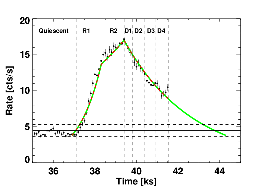

Using the following steps we then estimate the flare loop lengths:
- •
(slope of the EM-T evolution) : We divide the flare data into several time bins and obtain the emission-measure and temperature for the individual bins. In Fig.11 (upper panel), we show the EPIC pn light curve of the large flare observed on LO Peg together with the time intervals used for our spectroscopic analysis; the quiescent phase is also marked for reference. The first two spectra cover the flare rise and the following time intervals cover the different phases in the flare. Each of these spectra are fitted with a 4-T APEC model including the quiescent emission, i.e., the first two temperature components are fixed to the plasma properties of the quiescent phase before the flare. Thus we allow the third and fourth temperature component to vary independently, which accounts for the overall X-ray emission during the flare. In Fig. 11 (lower panel), we show the evolution of the fit parameters EM and T and measure a slope for the decaying phase of =0.560.35 in the EM-T plane.
- •
T (Flare peak temperature): The intrinsic flare peak temperature is obtained by applying (in units of K) to the observed maximum temperature; here the coefficients =0.16 and =1.16 have been derived using the energy response of the XMM-Newton EPIC detectors (Reale, 2007). Thus, the intrinsic flare temperature is estimated as 42.19 5.86 MK.
- •
(Flare decay time): We obtain the decay time by modeling the flare light curve. We assume an exponential growth and decay given by with the observed e-folding time of the flare’s light curve determined by fitting the light curve from the peak of the flare, until the count rate has reached 10 of the peak level. We extrapolate the light curve during the decay phase assuming an exponential decay of the count rate, since our LO Peg observations do not cover the entire flare, and obtain a decay time 3.260.43 ks.
We estimate a loop half length L 2.061.38 cm; assuming a stellar radius of 0.72 0.10 , we find a loop length L 0.41R⋆. Comparing the estimated loop length with the pressure scale height , defined as = , where T is the plasma temperature in the loop, is the molecular weight and g is the surface gravity of LO Peg (log g4.50.5, Pandey et al. 2005), and substituting these values in the expression for , we find a value of cm; thus the loop length obtained for LO Peg flare is smaller than the pressure scale height of the flaring plasma.
4.2.1 Flare energetics
A detailed assessment of the energy radiated in X-ray can be obtained using a simple integration of the instantaneous X-ray luminosity over the flare duration ( 5 ks), yielding a total energy radiated in the X-ray band of E 7.3 erg. Observations of solar flares show that the density of the flaring loop during the peak and the decay phase of the flare are close to the quasi-steady state values; we now assume that this is also the case for the flare on LO Peg. One of the simplest model to understand the stellar flare energetics is to assume that the heating function is constant in space, i.e., assume that it is independent of the local values of the flare loop temperature and pressure.
In this case we can apply the scaling laws for static loops derived by Rosner et al. (1978), i.e., the relation holds, where is the estimated loop length ( 2.06 1.38 cm) and p0 is the (constant) pressure appearing in the other scaling-law, Tmax= (p0 L). The total heating rate during flare peak is then erg/s, where we estimate the volume from the measured emission measure and density. Thus, the obtained heating rate is a factor of 6 higher than the flare’s X-ray luminosity obtained from spectral fitting. This difference in the heating rate and the flare X-ray luminosity is compatible with the fact that during a flaring state, the X-ray emission is only one of the possible energy loss terms; at flare temperatures we expect the energy losses by thermal conduction to be quite high.
5 Summary and conclusions
With its X-ray luminosity of LX=5.11029 erg/s in 0.2-10 keV band the low-mass ultrafast rotator LO Peg attains an activity level of log =-3.1, close to the saturation limit as expected, yet its (quiescent) X-ray light curve does show variability at 30-40 level, possibly due to rotational modulation. A large flare is observed toward the end of our observation, which leads to significant spectral changes in the X-ray emission as observed for other stars. At the onset of the flare, the optical emission peaks before the soft X-ray emission peak, and the recorded OM light curve follows approximately the time derivative of the soft X-ray emission, suggesting the presence of the Neupert effect and and the evaporation of chromospheric material as cause for the soft X-ray flare. We also find different maximum times for the harder and softer parts of the observed X-ray emission, indicating the thermal cooling of the heated plasma. The XMM-Newton data thus indicate that the general features of solar flare models also seem to apply to the flare observed on LO Peg.
The overall X-ray properties of LO Peg are quite similar to those of other active stars with dominant plasma components at temperatures of 3, 7.5 and 20 MK during quiescence and 3.5, 12 and 32 MK during the flare, when the emission measure of the hotter plasma increases significantly and higher temperatures are reached, while the cool plasma is only marginally changed. From the recorded X-ray light curves we infer loop lengths of the flaring plasma somewhat smaller than half the stellar radius, assuming that the flare has a simple geometry.
The coronal elemental abundances of LO Peg show an inverse-FIP effect. These abundances were obtained relative to solar-photospheric abundance, since there exist no measured photospheric abundances of LO Peg. A comparison of X-ray properties like the coronal temperature structure and the abundance pattern of LO Peg with other active fast rotators shows them to be very similar. The determined coronal Ne/O abundance ratios of LO Peg are also similar to other low-mass ultrafast rotators. We find no variation of the Ne/O ratio with activity level for our sample of very active rapid rotators.
Acknowledgements.
This work is based on observations obtained with XMM-Newton, an ESA science mission with instruments and contributions directly funded by the ESA Member States and the USA (NASA). S.L. acknowledges support from the DST INSPIRE Faculty fellowship.References
- Alexander (1997) Alexander, T. 1997, in Astrophysics and Space Science Library, Vol. 218, Astronomical Time Series, ed. D. Maoz, A. Sternberg, & E. M. Leibowitz, 163
- Arnaud (1996) Arnaud, K. A. 1996, in ASP Conf. Ser. 101: Astronomical Data Analysis Software and Systems V, ed. G. H. Jacoby & J. Barnes, 17–+
- Audard et al. (2003) Audard, M., Güdel, M., Sres, A., Raassen, A. J. J., & Mewe, R. 2003, A&A, 398, 1137
- Brinkman et al. (2001) Brinkman, A. C., Behar, E., Güdel, M., et al. 2001, A&A, 365, L324
- Coates et al. (1980) Coates, D. W., Halprin, L., Sartori, P., & Thompson, K. 1980, Information Bulletin on Variable Stars, 1849
- Dal & Tas (2003) Dal, H. A. & Tas, G. 2003, Information Bulletin on Variable Stars, 5390
- den Herder et al. (2001) den Herder, J. W., Brinkman, A. C., Kahn, S. M., et al. 2001, A&A, 365, L7
- Drake & Testa (2005) Drake, J. J. & Testa, P. 2005, Nature, 436, 525
- Eibe et al. (1999) Eibe, M. T., Byrne, P. B., Jeffries, R. D., & Gunn, A. G. 1999, A&A, 341, 527
- Favata et al. (1998) Favata, F., Micela, G., Sciortino, S., & D’Antona, F. 1998, A&A, 335, 218
- Gabriel & Jordan (1969) Gabriel, A. H. & Jordan, C. 1969, MNRAS, 145, 241
- Grevesse & Sauval (1998) Grevesse, N. & Sauval, A. J. 1998, Space Sci. Rev., 85, 161
- Güdel et al. (2001) Güdel, M., Audard, M., Magee, H., et al. 2001, A&A, 365, L344
- Guirado et al. (2011) Guirado, J. C., Marcaide, J. M., Martí-Vidal, I., et al. 2011, A&A, 533, A106
- Haisch et al. (1983) Haisch, B. M., Linsky, J. L., Bornmann, P. L., et al. 1983, ApJ, 267, 280
- Hussain et al. (2012) Hussain, G. A. J., Brickhouse, N. S., Dupree, A. K., et al. 2012, MNRAS, 423, 493
- Innis et al. (1984) Innis, J. L., Coates, D. W., & Thompson, K. 1984, Proceedings of the Astronomical Society of Australia, 5, 540
- Jansen et al. (2001) Jansen, F., Lumb, D., Altieri, B., et al. 2001, A&A, 365, L1
- Jeffries et al. (1994) Jeffries, R. D., Byrne, P. B., Doyle, J. G., et al. 1994, MNRAS, 270, 153
- Jeffries & Jewell (1993a) Jeffries, R. D. & Jewell, S. J. 1993a, MNRAS, 264, 106
- Jeffries & Jewell (1993b) Jeffries, R. D. & Jewell, S. J. 1993b, MNRAS, 264, 106
- Kron (1952) Kron, G. E. 1952, ApJ, 115, 301
- Kurster (1995) Kurster, M. 1995, in Lecture Notes in Physics, Berlin Springer Verlag, Vol. 454, IAU Colloq. 151: Flares and Flashes, ed. J. Greiner, H. W. Duerbeck, & R. E. Gershberg, 423
- Lalitha et al. (2013) Lalitha, S., Fuhrmeister, B., Wolter, U., et al. 2013, A&A, 560, A69
- Malina et al. (1994) Malina, R. F., Marshall, H. L., Antia, B., et al. 1994, AJ, 107, 751
- Mason et al. (2001) Mason, K. O., Breeveld, A., Much, R., et al. 2001, A&A, 365, L36
- Montes et al. (2001) Montes, D., López-Santiago, J., Gálvez, M. C., et al. 2001, MNRAS, 328, 45
- Neupert (1968) Neupert, W. M. 1968, ApJ, 153, L59
- Pallavicini et al. (1981) Pallavicini, R., Golub, L., Rosner, R., et al. 1981, ApJ, 248, 279
- Pandey et al. (2005) Pandey, J. C., Singh, K. P., Drake, S. A., & Sagar, R. 2005, AJ, 130, 1231
- Perryman et al. (1997) Perryman, M. A. C., Lindegren, L., Kovalevsky, J., et al. 1997, A&A, 323
- Pettersen (1976) Pettersen, B. R. 1976, Institute of Theoretical Astrophysics Blindern Oslo Reports, 46, 1
- Pizzolato et al. (2003) Pizzolato, N., Maggio, A., Micela, G., Sciortino, S., & Ventura, P. 2003, A&A, 397, 147
- Pradhan & Shull (1981) Pradhan, A. K. & Shull, J. M. 1981, ApJ, 249, 821
- Reale (2002) Reale, F. 2002, in Astronomical Society of the Pacific Conference Series, Vol. 277, Stellar Coronae in the Chandra and XMM-NEWTON Era, ed. F. Favata & J. J. Drake, 103
- Reale (2007) Reale, F. 2007, A&A, 471, 271
- Robrade & Schmitt (2005) Robrade, J. & Schmitt, J. H. M. M. 2005, A&A, 435, 1073
- Rosner et al. (1985) Rosner, R., Golub, L., & Vaiana, G. S. 1985, ARA&A, 23, 413
- Rosner et al. (1978) Rosner, R., Tucker, W. H., & Vaiana, G. S. 1978, ApJ, 220, 643
- Schmelz et al. (2005) Schmelz, J. T., Nasraoui, K., Roames, J. K., Lippner, L. A., & Garst, J. W. 2005, ApJ, 634, L197
- Serio et al. (1991) Serio, S., Reale, F., Jakimiec, J., Sylwester, B., & Sylwester, J. 1991, A&A, 241, 197
- Smith et al. (2001) Smith, R. K., Brickhouse, N. S., Liedahl, D. A., & Raymond, J. C. 2001, in ASP Conf. Ser. 247: Spectroscopic Challenges of Photoionized Plasmas, ed. G. Ferland & D. W. Savin, 161–+
- Stelzer et al. (2002) Stelzer, B., Burwitz, V., Audard, M., et al. 2002, A&A, 392, 585
- Stelzer & Neuhäuser (2000) Stelzer, B. & Neuhäuser, R. 2000, A&A, 361, 581
- Strüder et al. (2001) Strüder, L., Briel, U., Dennerl, K., et al. 2001, A&A, 365, L18
- Taš (2011) Taš, G. 2011, Astronomische Nachrichten, 332, 57
- Turner et al. (2001) Turner, M. J. L., Abbey, A., Arnaud, M., et al. 2001, A&A, 365, L27
- Voges et al. (1999) Voges, W., Aschenbach, B., Boller, T., et al. 1999, A&A, 349, 389
- Wolter et al. (2008) Wolter, U., Robrade, J., Schmitt, J. H. M. M., & Ness, J. U. 2008, A&A, 478, L11
- Young et al. (1990) Young, A., Skumanich, A., MacGregor, K. B., & Temple, S. 1990, ApJ, 349, 608
- Young (2005) Young, P. R. 2005, A&A, 444, L45
- Zuckerman & Song (2004) Zuckerman, B. & Song, I. 2004, ARA&A, 42, 685
- Zuckerman & Webb (2000) Zuckerman, B. & Webb, R. A. 2000, ApJ, 535, 959