Statistical inference for moving-average Lévy-driven processes: Fourier-based approach

Generally speaking, continuous-time Lévy-driven moving average processes are defined as

where $\mathcal{K}$ is a deterministic kernel and $L=(L_{t})_{t\in\mathbb{R}}$ is a two-sided Lévy process with Lévy triplet $(\gamma,\sigma,\nu)$. The conditions which guarantee that this integral is well-defined are given in the pioneering work by Rajput and Rosinski [6]. For instance, if $\int x^{2}\nu(dx)<\infty$, it is sufficient to assume that $\mathcal{K}\in\mathcal{L}^{1}({\mathbb{R}})\cap\mathcal{L}^{2}({\mathbb{R}})$. Some popular choices for the kernel are $\mathcal{K}(t)=t^{\alpha}e^{-\lambda t}1_{[0,\infty)}(t)$ with $\lambda>0$ and $\alpha>-1/2$, (Gamma-kernels, see e.g. Barndorff-Nielsen and Schmiegel [1]), or $\mathcal{K}(t)=e^{-\lambda|t|}$ (well-balanced Ornstein-Uhlenbeck process, see Schnurr and Woerner [7]).

Recently, Belomestny, Panov and Woerner [3] consider the statistical estimation of the Lévy measure $\nu$ from the low-frequency observations of the process $(Z_{t})$. The approach presented in [3] is rather general - in particular, it works well under various choices of $\mathcal{K}$. Nevertheless, this approach is based on the superposition of the Mellin and Fourier transforms of the Lévy measure, and therefore its practical implementation can meet some computational difficulties.

In this paper, we present another method, which essentially uses the fact that in some cases there exists a direct relation between the characteristic exponent of the process $L$ and the characteristic function of the process $Z.$ Therefore, the characteristic exponent can be estimated from the observations of the process $Z,$ and further application of the Fourier techniques from Belomestny and Reiss [2] and Panov [5] leads to the construction of a consistent estimator of the Lévy triplet.

The paper is organised as follows. In the next session, we provide the specifications of our model. In Section 3, we present the key mathematical idea, which lies in the core of the estimation procedure presented in Section 4. The upper and lower error bounds for the proposed estimates are given in Section 5. Joint consideration of the corresponding results, Theorems 1 and 2, yields the optimality of the estimates. Finally, in Section 6, we illustrate our approach with some numerical examples. All proofs are collected in Section 7.

In this work, we consider the integrals of the form (1), where $\mathcal{K}$ is a symmetric kernel of the form:

for some $\alpha\in(0,1).$ As a limiting case for $\alpha\searrow 0,$ we get the exponential kernel $\mathcal{K}_{0}(x)=\exp(-x).$ Here, for simplicity, we restrict our attention to a particular class of two-sided Lévy processes with jumps represented by a compound Poisson process $CPP_{t}$,

where $\gamma\in{\mathbb{R}}$ is a drift, $\sigma\geq 0$, $W_{t}$ is a Brownian motion, $N_{t}^{(1)},N_{t}^{(2)},$ are 2 Poisson processes with intensity $\lambda$, $Y_{1}^{(1)},Y_{2}^{(1)},...$ and $Y_{1}^{(2)},Y_{2}^{(2)},...$ are i.i.d. r.v’s with absolutely continuous distribution, and all $Y$’s, $N^{(1)}_{t},$ $N^{(2)}_{t}$, $W_{t}$ are jointly independent. Due to the Lévy-Khintchine formula, the characteristic exponent of $L$ is given by

where $\nu$ is a Lévy measure of $(L_{t})$, and $\mathcal{F}[\nu](u)=\int_{{\mathbb{R}}}e^{iux}\nu(dx)$ stands for the Fourier transform of $\nu.$

It is important to note that the process $\left(Z_{t}\right)_{t\in\mathbb{R}}$ is strictly stationary with the characteristic function of the form

and therefore for any time points $t_{1},...,t_{n},$ the r.v.’s $Z_{t_{1}},...,Z_{t_{n}}$ are identically distributed (but dependent). Our aim is to estimate the Lévy triplet $(\gamma,\sigma,\nu)$ based on the equidistant observations of the process $Z_{t}$ at the time points $\Delta,2\Delta,..,n\Delta,$ where $\Delta>0$ is fixed (low-frequency set-up).

The key observation is that under our choice of the kernel function $\mathcal{K},$ we can represent the characteristic exponent $\psi(\cdot)$ of the process $(L_{t})$ via the characteristic function $\Phi(\cdot)$ of the process $Z_{t}$. More precisely, since

we have

Therefore, we derive

since $\psi(u)u^{\alpha-1}\to 0$ as $u\to+0$ provided that $\int|x|\nu(dx)<\infty$, see Lemma 1. Therefore, the characteristic exponent $\psi$ can be directly estimated from data via a plug-in estimator based on the empirical characteristic function of $Z$.

Moreover, returning to the representation (5), we conclude that the Lévy triplet $(\gamma,\sigma,\nu)$ can be estimated from $\psi.$ In fact, since $\nu$ is absolutely continuous with an absolutely integrable density, then by the Riemann-Lebesgue lemma (see [4], p. 43) $\mathcal{F}[\nu](u)\to 0$ as $|u|\to\infty,$ and consequently $\psi(u)$ can be viewed, at least for large $|u|,$ as a second order polynomial with the coefficients $(-\lambda,i\gamma,-\sigma^{2}/2).$ This observation gives rise for the estimation procedure, which we present in the next session.

Assume that the process $(Z_{t})$ is observed on the equidistant time grid $t\in\left\{\Delta,2\Delta,...,n\Delta\right\},$ where $\Delta$ is fixed.

Step 1: estimation of $\psi$. Define

and set

where the branch of the complex logarithm is taken in such a way that $\psi_{n}$ is continuous on $(-x_{0,n},x_{0,n})$ with $\psi_{n}(0)=0$ and $x_{0,n}$ being the first zero of $\Phi_{n}.$ In fact, since $\Phi$ does not vanish on $\mathbb{R}$, we have $x_{0,n}\stackrel{{\scriptstyle a.s.}}{{\to}}\infty.$

Step 2: estimation of $\sigma$ and $\lambda$. Let $U_{n}\to\infty$ and

where $\widetilde{w}(u)$ is a continuous function, supported on the interval $[\varepsilon,1]$ with some $\varepsilon>0.$ Consider now the optimisation problem

which has the solution

with

Note that the weighting function $w_{\sigma}^{U_{n}}(u)$ satisfies the property $w_{\sigma}^{U_{n}}(u)=U_{n}^{-3}w_{\sigma}^{1}(u/U_{n})$, and moreover,

Analogously,

holds with $w_{\lambda}^{U_{n}}(u)=U_{n}^{-1}w_{\lambda}^{1}(u/U_{n})$ satisfying the properties

Step 3: estimation of $\gamma$. Finally, the parameter $\gamma$ can be estimated by considering the optimisation problem

which leads to the estimate

where $w_{\gamma}^{U_{n}}(u)=U_{n}^{-2}w_{\gamma}^{1}(u/U_{n})$ fulfills $\int_{0}^{U_{n}}u\,w_{\gamma}^{U_{n}}(u)\,du=1.$ All functions $w_{\sigma}^{1}$, $w_{\gamma}^{1}$ and $w_{\lambda}^{1}$ are supported on $[\varepsilon,1]$ and bounded.

Step 4: estimation of the Lévy density. Note that under our assumptions on the Lévy process $(L_{t})$ (see Section 2), the Levy measure $\nu$ possesses a density, which we denote, with a slight abuse of notation, also by $\nu(x)$. This Lévy density can be estimated as a regularised inverse Fourier transform of the remainder:

where $w_{\nu}$ is a weight function supported on $[-1,1].$ Note that $\int_{{\mathbb{R}}}\nu_{n}(x)\,dx=\lambda_{n},$ if $w_{\nu}(0)=1.$

As shown in the next theorem, the above rates are optimal in minimax sense.

Consider the integral (1) with the kernel $\mathcal{K}(x)$ from the class (2), and the Lévy process $(L_{t})$ defined by (3)-(4). For simulation study, we take $\gamma=5,$ $\lambda=1$ and $\sigma=0$, and aim to estimate these parameters under different choices of the parameter $\alpha$, namely $\alpha=0.5,$ $0.8$ and $0.9$.

Simulation. For $k=1,2$, denote the jump times of $L_{t}^{(k)}$ by $s_{1}^{(k)},s_{2}^{(k)},....$, corresponding to the jump sizes $Y_{1}^{(k)},Y_{2}^{(k)},...$ Note that

where

Estimation. Following the ideas from Section 4, we estimate the parameters $\gamma,\lambda,\sigma$ under different choices of $\alpha.$

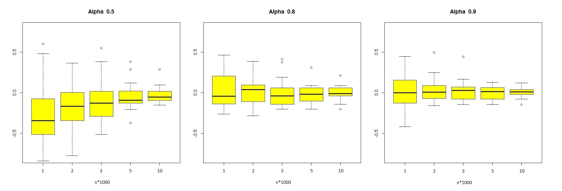
To show the convergence properties of the considered estimates, we provide simulations with different values of $n$. The boxplots of the corresponding estimation errors (differences) based on 25 simulation runs are presented on Figures 2, 3 and 4. Note that the parameter $U_{n}$ is chosen by numerical optimisation. The exact values are presented in Tables 1 and 2.

The simulation study illustrates our theoretical results on the rates of convergence given in Section 5. In fact, visual comparison of Figures 2, 3 and 4 shows that the proposed estimator for the parameter $\sigma$ has the highest speed of convergence to the true value, whereas the corresponding speed for $\gamma_{n}$ is lower, and for $\lambda_{n}$ even more low (cf with the rates in Theorem 1). Moreover, the simulations results show that the convergence rates significantly depend on the parameter $\alpha$. More precisely, it turns out that the quality of estimation increases with growing $\alpha$, and the best rates correspond to the case when $\alpha$ is close to 1. This can explained by the fact that observations become less independent as $\alpha$ increases.

References

- [1] Barndorff-Nielsen, Ole E. and Schmiegel, J. Brownian semistationary processes and volatility/intermittency. In Advanced financial modelling, volume 8 of Radon Ser. Comput. Appl. Math., pages 1–25. Walter de Gruyter, Berlin, 2009.
- [2] Belomestny, D., and Reiss, M. Estimation and Calibration of Lévy Models via Fourier Methods. In Lévy Matters IV: Estimation for Discretely Observed Lévy Processes, pages 1–76. Springer International Publishing, Cham, 2015.
- [3] Belomestny, D., Panov, V., and Woerner, J. Low frequency estimation of continuous-time moving average Lévy processes. arXiv: 1607.00896, 2016.
- [4] Kawata, T. Fourier analysis in probability theory. Academic Press, 1972.
- [5] Panov, V. Abelian theorems for stochastic volatility models and semiparametric estimation of the signal space. PhD thesis, Humboldt University, 2012.
- [6] Rajput, B. and Rosiński, J. Spectral representations of infinitely divisible processes. Probability Theory and Related Fields, 82(3):451–487, 1989.
- [7] Schnurr, A. and Woerner, J. H. C. Well-balanced Lévy driven Ornstein-Uhlenbeck processes. Stat. Risk Model., 28(4):343–357, 2011.
- [8] Tsybakov, A. Introduction to nonparametric estimation. Springer, New York, 2009.