Proving linearizability using forward simulations

Programs interact with libraries by calling named library methods, which receive parameter values and yield return values upon completion. We fix arbitrary sets ${\mathbb{M}}$ and ${\mathbb{V}}$ of method names and parameter/return values. We fix an arbitrary set ${\mathbb{O}}$ of operation identifiers, and for given sets ${\mathbb{M}}$ and ${\mathbb{V}}$ of methods and values, we fix the sets

A library is an LTS over alphabet $\Sigma$ such that $C\cup R\subseteq\Sigma$. We assume that the traces of a library satisfy standard well-formedness properties, e.g., return actions correspond to previous call actions, which for lack of space are delegated to Appendix 0.A. An operation $k$ is called completed in a trace $\tau$ when $ret(m,d,k)$ occurs in $\tau$, for some $m$ and $d$. Otherwise, it is called pending.

The projection of a library trace over $C\cup R$ is called a history. The set of histories of a library $L$ is denoted by $H(L)$. Since libraries only dictate methods’ executions between their respective calls and returns, for any history they admit, they must also admit histories with weaker inter-operation ordering, in which calls may happen earlier, and/or returns later. A history $h_{1}$ is weaker than a history $h_{2}$, written $h_{1}\sqsubseteq h_{2}$, iff there exists a history $h_{1}^{\prime}$ obtained from $h_{1}$ by appending return actions, and deleting call actions, s.t.: $h_{2}$ is a permutation of $h_{1}^{\prime}$ that preserves the order between return and call actions, i.e., if a given return action occurs before a given call action in $h_{1}^{\prime}$, then the same holds in $h_{2}$.

A library $L$ is called atomic when there exists a set $S$ of sequential histories such that $H(L)$ contains every weakening of a history in $S$. Atomic libraries are often considered as specifications for concurrent objects. Libraries can be made atomic by guarding their methods bodies with global lock acquisitions.

A library $L$ is called a queue implementation when $\mathchoice{\mbox{${\mathbb{M}}$}}{\mbox{${\mathbb{M}}$}}{\mbox{\scriptsize${\mathbb{M}}$}}{\mbox{\tiny${\mathbb{M}}$}}=\{enq,deq\}$ ($enq$ is the method that enqueues a value and $deq$ is the method removing a value) and $\mathchoice{\mbox{${\mathbb{V}}$}}{\mbox{${\mathbb{V}}$}}{\mbox{\scriptsize${\mathbb{V}}$}}{\mbox{\tiny${\mathbb{V}}$}}=\mathchoice{\mbox{${\mathbb{N}}$}}{\mbox{${\mathbb{N}}$}}{\mbox{\scriptsize${\mathbb{N}}$}}{\mbox{\tiny${\mathbb{N}}$}}\cup\{{\tt EMPTY}\}$ where EMPTY is the value returned by $deq$ when the queue is empty. Similarly, a library $L$ is called a stack implementation when $\mathchoice{\mbox{${\mathbb{M}}$}}{\mbox{${\mathbb{M}}$}}{\mbox{\scriptsize${\mathbb{M}}$}}{\mbox{\tiny${\mathbb{M}}$}}=\{push,pop\}$ and $\mathchoice{\mbox{${\mathbb{V}}$}}{\mbox{${\mathbb{V}}$}}{\mbox{\scriptsize${\mathbb{V}}$}}{\mbox{\tiny${\mathbb{V}}$}}=\mathchoice{\mbox{${\mathbb{N}}$}}{\mbox{${\mathbb{N}}$}}{\mbox{\scriptsize${\mathbb{N}}$}}{\mbox{\tiny${\mathbb{N}}$}}\cup\{{\tt EMPTY}\}$. For queue and stack implementations, we assume that the same value is never added twice, i.e., for every trace $\tau$ of such a library and every two call actions $inv(m,d_{1},k_{1})$ and $inv(m,d_{2},k_{2})$ where $m\in\{enq,push\}$ we have that $d_{1}\neq d_{2}$. As shown in several works [2, 6], this assumption is without loss of generality for libraries that are data independent, i.e., their behaviors are not influenced by the values added to the collection, which is always the case in practice. On a technical note, this assumption is used to define ($\Gamma$-)deterministic abstract implementations of stacks and queues in Section 4 and Section 5.

Conformance of a library $L_{1}$ to a specification given as an “abstract” library $L_{2}$ is formally captured by (observational) refinement. Informally, we say $L_{1}$ refines $L_{2}$ iff every computation of every program using $L_{1}$ would also be possible were $L_{2}$ used instead. We assume that a program can interact with the library only through call and return actions, and thus refinement can be defined as history set inclusion. Refinement is equivalent to the linearizability criterion [17] when $L_{2}$ is an atomic library [11, 7].

Linearizability [17] requires that every history of a concurrent library $L_{1}$ can be “linearized” to a sequential history admitted by a library $L_{2}$ used as a specification. Formally, a sequential history $h_{2}$ with only complete operations is called a linearization of a history $h_{1}$ when $h_{1}\sqsubseteq h_{2}$. A history $h_{1}$ is linearizable w.r.t. a library $L_{2}$ iff there exists a linearization $h_{2}$ of $h_{1}$ such that $h_{2}\in H(L_{2})$. A library $L_{1}$ is linearizable w.r.t. $L_{2}$, written $L_{1}\sqsubseteq L_{2}$, iff each history $h_{1}\in H(L_{1})$ is linearizable w.r.t. $L_{2}$.

In the rest of the paper, we discuss methods for proving refinement (and thus, linearizability) focusing mainly on queue and stack implementations.

We describe $\mathit{HWQ}$ where the linearization points of the enqueue methods are not fixed. The shared state consists of an array items storing the values in the queue and a counter back storing the index of the first unused position in items. Initially, all the positions in the array are null and back is 0. An enqueue method starts by reserving a position in items (i stores the index of this position and back is incremented so the same position can’t be used by other enqueues) and then, stores the input value x at this position. The dequeue method traverses the array items starting from the beginning and atomically swaps null with the encountered value. If the value is not null, then the dequeue returns that value. If it reaches the end of the array, then it restarts.

The linearization points of the enqueues are not fixed, they depend on dequeues executing in the future. Consider the following trace with two concurrent enqueues (${\tt i}(k)$ represents the value of i in operation $k$): $inv(enq,x,1)$, $inv(enq,y,2)$, ${\tt i}(1)=\mbox{{\tt bck++}}$, ${\tt i}(2)=\mbox{{\tt bck++}}$, ${\tt items[i(}2{\tt)]}=y$. Assuming that the linearization point corresponds to the assignment of i, the history of this trace should be linearized to $inv(enq,x,1)$, $ret(enq,1)$, $inv(enq,y,2)$, $ret(enq,2)$. However, a dequeue executing until completion after this trace will return $y$ (only position $1$ is filled in the array items) which is not consistent with this linearization. On the other hand, assuming that enqueues should be linearized at the assignment of items[i] and extending the trace with ${\tt items[i(}1{\tt)]}=x$ and a completed dequeue that in this case returns $x$, leads to the incorrect linearization: $inv(enq,y,2)$, $ret(enq,2)$, $inv(enq,x,1)$, $ret(enq,1)$, $inv(deq,3)$, $ret(deq,x,3)$.

The dequeue method has a fixed linearization point which corresponds to an execution of swap returning a non-null value. This action alone contributes to the effect of that value being removed from the queue. Every concurrent history can be linearized to a sequential history where dequeues occur in the order of their linearization points in the concurrent history. This claim is formally proved in Section 4.3.

Since the linearization points of the enqueues are not fixed, there exists no forward simulation from $\mathit{HWQ}$ to $AbsQ_{0}$. In the following, we describe the abstract implementation $AbsQ$ for which such a forward simulation does exist.

Informally, $AbsQ$ records the happens-before order between enqueue operations for which the added value has not been removed by a dequeue operation. The linearization point of a dequeue operation with return value $d\neq{\tt EMPTY}$ is enabled only if the happens-before stored in the current state contains a minimal enqueue that adds the value $d$. The effect of the linearization point is that the minimal enqueue is removed from the current state and the return value is recorded in the library state. When the return value is EMPTY, the linearization point of a dequeue is enabled only if the current state stores only pending enqueues (the dequeue overlaps with all the enqueue operations stored in the current state and it can be linearized before all of them). The return of a dequeue is enabled only if the returned value matches the one fixed at the linearization point.

Figure 2 pictures two executions of $AbsQ$ for two extended histories (that include dequeue linearization points). The state of $AbsQ$ after each action is pictured as a graph below the action. The nodes of this graph represent enqueue operations and the edges happens-before constraints. Each node is labeled by a value (the input of the enqueue) and a flag PEND or COMP showing whether the operation is pending or completed. For instance, in the case of the first history, the dequeue linearization point $lin(deq,y,3)$ is enabled because the current happens-before contains a minimal enqueue operation with input $y$. Note that a linearization point $lin(deq,x,3)$ is also enabled at this state.

Formally, the states of $AbsQ$ are tuples $\langle{O,<,\ell,rv,cp}\rangle$ where $O\subseteq\mathchoice{\mbox{${\mathbb{O}}$}}{\mbox{${\mathbb{O}}$}}{\mbox{\scriptsize${\mathbb{O}}$}}{\mbox{\tiny${\mathbb{O}}$}}$ is a set of operation identifiers, $<\subseteq O\times O$ is a strict partial order, $\ell:O\mathbin{\rightarrow}\mathchoice{\mbox{${\mathbb{V}}$}}{\mbox{${\mathbb{V}}$}}{\mbox{\scriptsize${\mathbb{V}}$}}{\mbox{\tiny${\mathbb{V}}$}}\times\{\tt{PEND,\tt{COMP}}\}$ labels every identifier with a value and a pending/completed flag (the flag is used to track the happens-before order), $rv:\mathchoice{\mbox{${\mathbb{O}}$}}{\mbox{${\mathbb{O}}$}}{\mbox{\scriptsize${\mathbb{O}}$}}{\mbox{\tiny${\mathbb{O}}$}}{}\mathbin{\rightharpoonup}\mathchoice{\mbox{${\mathbb{V}}$}}{\mbox{${\mathbb{V}}$}}{\mbox{\scriptsize${\mathbb{V}}$}}{\mbox{\tiny${\mathbb{V}}$}}$ records the return value of a dequeue fixed at its linearization point (${}\mathbin{\rightharpoonup}$ denotes a partial function), and $cp:\mathchoice{\mbox{${\mathbb{O}}$}}{\mbox{${\mathbb{O}}$}}{\mbox{\scriptsize${\mathbb{O}}$}}{\mbox{\tiny${\mathbb{O}}$}}{}\mathbin{\rightharpoonup}\{A_{1},A_{2},R_{1},R_{2},R_{3}\}$ records the control point of every enqueue ($A_{1},A_{2}$) or dequeue operation ($R_{1},R_{2},R_{3}$). All the components are $\emptyset$ in the initial state, and the transition relation $\mathbin{\rightarrow}$ is defined in Fig. 3. The alphabet of $AbsQ$ contains call/return actions and dequeue linearization points, denoted by $lin(deq,d,k)$. $Lin(deq)$ is the set of all actions $lin(deq,d,k)$.

Concerning enqueue operations, the rule call-enq orders the invoked operation after all the completed enqueues in the current state, and the rules ret-enq1/ret-enq2 flip the corresponding flag from PEND to COMP provided that the operation is still present in the current state. For dequeue operations, call-deq only increments the control point and ret-deq checks whether the return value is the same as the one fixed at the linearization point. The linearization point rule lin-deq1 corresponds to the case of a non-empty queue, showing that $lin(deq,d,k)$ is enabled only if $d$ has been added by an enqueue which is minimal in the current happens-before. When enabled, it removes the enqueue adding $d$ from the state. The linearization point rule lin-deq2 corresponds to the case of dequeue operations linearized with an EMPTY return value.

The following result states that the library $AbsQ$ has exactly the same set of histories as the standard abstract library $AbsQ_{0}$ (see Appendix 0.C for a proof).

A trace of a queue implementation is called $Lin(deq)$-complete when every completed dequeue has a linearization point, i.e., each return action $ret(deq,d,k)$ is preceded by an action $lin(deq,d,k)$. A queue implementation $L$ over alphabet $\Sigma$, such that $C\cup R\cup Lin(deq)\subseteq\Sigma$, is called with fixed dequeue linearization points when every trace $\tau\in Tr(L)$ is $Lin(deq)$-complete.

The following result shows that $C\cup R\cup Lin(deq)$-forward simulations are a sound and complete proof method for showing the correctness of a queue implementation with fixed dequeue linearization points (up to the correctness of the linearization points). It is obtained from Theorem 4.1 and Theorem 3.1 using the fact that the alphabet of $AbsQ$ is exactly $C\cup R\cup Lin(deq)$ and $AbsQ$ is deterministic.

We describe a forward simulation $\mathit{fs}_{1}$ from $\mathit{HWQ}$ to $AbsQ$. A $\mathit{HWQ}$ state is related by $\mathit{fs}_{1}$ to an $AbsQ$ state that consists of all the enqueue operations for which the input is still present in the array items and all the pending enqueue operations that have at most reserved an array position, ordered by a relation $<$ satisfying the following:

• (a)

  pending enqueues are maximal, i.e., for every two enqueues $k$ and $k^{\prime}$ such that $k^{\prime}$ is pending, we have that $k^{\prime}\not<k$,

• (b)

  $<$ is consistent with the order in which positions of items have been reserved, i.e., for every two enqueues $k$ and $k^{\prime}$ such that ${\tt i}(k)<{\tt i}(k^{\prime})$, we have that $k^{\prime}\not<k$,

• (c)

  an enqueue which has reserved a position $i$ can’t be ordered before another enqueue that has reserved a position $j\geq i$ when the position $i$ has been “observed” by a non-linearized dequeue that may “observe” $j$ in the current array traversal, i.e., for every two enqueues $k$ and $k^{\prime}$, and a dequeue $k_{d}$, such that

  $\displaystyle\hskip-22.76219pt{\tt x}(k_{d})={\tt null}\land{\tt i}(k^{\prime})\leq{\tt range}(k_{d})\land{\tt i}(k)\leq{\tt i}(k_{d})\leq{\tt i}(k^{\prime})\land({\tt i}(k)={\tt i}(k_{d})\mathbin{\Rightarrow}k_{d}@{\tt if}\text{-}{\tt inc})$

  (1)

  we have that $k\not<k^{\prime}$. The predicate $k_{d}@{\tt if}\text{-}{\tt inc}$ holds when the dequeue $k_{d}$ is at a control point after a swap returning null and before the increment of i.

We show that $\mathit{fs}_{1}$ is indeed a $C\cup R\cup Lin(deq)$-forward simulation. Let $s$ and $t$ be states of $\mathit{HWQ}$ and $AbsQ$, respectively, such that $(s,t)\in\mathit{fs}_{1}$. We omit discussing the trivial case of transitions labeled by call and return actions which are simulated by similar transitions of $AbsQ$ (for the return a dequeue operation $k$, we use the equality between the local variable ${\tt x}(k)$ in $s$ and the component $rv(k)$ in $t$).

We show that each internal step of an enqueue or dequeue, except the execution of swap returning a non-null value in dequeue (which represents its linearization point), is simulated by an empty sequence of $AbsQ$ transitions, i.e., for every state $s^{\prime}$ obtained through one of these steps, if $(s,t)\in\mathit{fs}_{1}$, then $(s^{\prime},t)\in\mathit{fs}_{1}$ for each $AbsQ$ state $t$. Essentially, this consists in proving the following property, called monotonicity: the set of possible orders $<$ associated by $\mathit{fs}_{1}$ to $s^{\prime}$ doesn’t exclude any order $<$ associated to $s$.

Concerning enqueues, let $s^{\prime}$ be the state obtained from $s$ when a pending enqueue $k$ reserves an array position. This enqueue must be maximal in both $t$ and any state $t^{\prime}$ related to $s^{\prime}$ (since it’s pending). Moreover, there is no dequeue that can “observe” this position before restarting the array traversal. Therefore, item (c) in the definition of $<$ doesn’t constrain the order between $k$ and some other enqueue neither in $s$ nor in $s^{\prime}$. Since this transition doesn’t affect the constraints on the order between enqueues different from $k$ (their local variables remain unchanged), monotonicity holds. This property is trivially satisfied by the second step of enqueue which doesn’t affect i.

To prove monotonicity in the case of dequeue internal steps different from its linearization point, it is important to track the non-trivial instantiations of item (c) in the definition of $<$ over the two states $s$ and $s^{\prime}$, i.e., the triples $(k,k^{\prime},k_{d})$ for which (1) holds. Instantiations that are enabled only in $s^{\prime}$ may in principle lead to a violation of monotonicity (since they restrict the orders $<$ associated to $s^{\prime}$). For the two steps that begin an array traversal, i.e., reading the index of the last used position and setting i to $0$, there exist no such new instantiations in $s^{\prime}$ because the value of i is either not set or $0$. The same is true for the increment of i in a dequeue $k_{d}$ since the predicate $k_{d}@{\tt if}\text{-}{\tt inc}$ holds in state $s$. The execution of swap returning null in a dequeue $k_{d}$ enables new instantiations $(k,k^{\prime},k_{d})$ in $s^{\prime}$, thus adding potentially new constraints $k\not<k^{\prime}$. We show that these instantiations are however vacuous because $k$ must be pending in $s$ and thus maximal in every order $<$ associated by $\mathit{fs}_{1}$ to $s$. Let $k$ and $k^{\prime}$ be two enqueues such that together with the dequeue $k_{d}$ they satisfy the property (1) in $s^{\prime}$ but not in $s$. We write ${\tt i}_{s}(k)$ for the value of the variable i of operation $k$ in state $s$. We have that ${\tt i}_{s^{\prime}}(k)={\tt i}_{s^{\prime}}(k_{d})\leq{\tt i}_{s^{\prime}}(k^{\prime})$ and ${\tt items}[{\tt i}_{s^{\prime}}(k_{d})]={\tt null}$. The latter implies that the enqueue $k$ didn’t executed the second statement (since the position it reserved is still null) and it is pending in $s$. The step that checks that the value returned by swap is null doesn’t modify the variables in property (1) and also, it doesn’t change the valuation of the predicate $@{\tt if}\text{-}{\tt inc}$.

Finally, we show that the linearization point of a dequeue $k$ of $\mathit{HWQ}$, i.e., an execution of swap returning a non-null value $d$, from state $s$ and leading to a state $s^{\prime}$ is simulated by a transition labeled by $lin(deq,d,k)$ of $AbsQ$ from state $t$. By the definition of $\mathit{HWQ}$, there is a unique enqueue $k_{e}$ which filled the position updated by $k$, i.e., ${\tt i}_{s}(k_{e})=i_{s}(k)$ and ${\tt x}_{s^{\prime}}(k)={\tt x}_{s}(k_{e})$. We show that $k_{e}$ is minimal in the order $<$ of $t$ which implies that $lin(deq,d,k)$ is enabled in $t$. Thus, instantiating item (c) in the definition of $<$ with $k^{\prime}=k_{e}$ and $k_{d}=k$ we get that every enqueue that reserved a position smaller than the one of $k_{e}$ can’t be ordered before $k_{e}$ in the order $<$. Also, applying item (b) with $k=k_{e}$ we get the same for every enqueue that reserved a bigger position. An enqueue that didn’t reserved a position is by definition maximal in $<$ and therefore, not a predecessor of $k_{e}$. Then, the state $t^{\prime}$ obtained from $t$ through a $lin(deq,d,k)$ transition is related to $s^{\prime}$ because (1) the value added by $k_{e}$ is not anymore present in items which implies that $k_{e}$ doesn’t occur in any $AbsQ$ state related to $s^{\prime}$, and (2) the value of ${\tt x}(k)$ is set to $d\neq{\tt null}$ which implies that $rv(k)$ is set to $d$ in every $AbsQ$ state related to $s^{\prime}$.

We explain the meaning of the commit points on a simplified version of the Time-Stamped Stack [9] ($\mathit{TSS}$, for short) given in Figure 4. This implementation maintains an array of singly-linked lists, one for each thread, where list nodes contain a data value (field data), a timestamp (field ts), the next pointer (field next), and a boolean flag indicating whether the node represents a value removed from the stack (field taken). Initially, each list contains a sentinel dummy node pointing to itself with timestamp $-1$ and the flag taken set to false.

Pushing a value to the stack proceeds in several steps: adding a node with maximal timestamp in the list associated to the thread executing the push (given by the special variable myTID), asking for a new timestamp (given by the shared variable TS), and updating the timestamp of the added node. Popping a value from the stack consists in traversing all the lists, finding the first element which doesn’t represent a removed value (i.e., taken is false) in each list, and selecting the element with the maximal timestamp. A compare-and-swap (CAS) is used to set the taken flag of this element to true. The procedure restarts if the CAS fails.

The push operations don’t have a fixed linearization point because adding a node to a list and updating its timestamp are not executed in a single atomic step. The nodes can be added in an order which is not consistent with the order between the timestamps assigned later in the execution. Also, the value added by a push that just added an element to a list can be popped before the value added by a completed push (since it has a maximal timestamp). The same holds for pop operations: The only reasonable choice for a linearization point is a successful CAS (that results in updating the field taken). Fig. 5 pictures an execution showing that this action doesn’t correspond to a linearization point, i.e., an execution for which the pop operations in every correct linearization are not ordered according to the order between successful CASs. In every correct linearization of that execution, the pop operation removing $x$ is ordered before the one removing $z$ although they perform a successful CAS in the opposite order.

An interesting property of the successful CASs in pop operations is that they fix the return value, i.e., the return value is youngest->data where youngest is the node updated by the CAS. We call such actions commit points. More generally, commit points are actions that access shared variables, from which every control-flow path leads to the return control point and contains no more accesses to the shared memory (i.e., after a commit point, the return value is computed using only local variables).

When the commit points of pop operations are fixed to particular implementation actions (e.g., a successful CAS) we assume that the library is an LTS over an alphabet that contains actions $com(pop,d,k)$ with $d\in\mathchoice{\mbox{${\mathbb{V}}$}}{\mbox{${\mathbb{V}}$}}{\mbox{\scriptsize${\mathbb{V}}$}}{\mbox{\tiny${\mathbb{V}}$}}$ and $k\in\mathchoice{\mbox{${\mathbb{O}}$}}{\mbox{${\mathbb{O}}$}}{\mbox{\scriptsize${\mathbb{O}}$}}{\mbox{\tiny${\mathbb{O}}$}}$ (denoting the commit point of the pop with identifier $k$ and returning $d$). Let $Com(pop)$ be the set of such actions.

We define an abstract stack $AbsS$ over alphabet $C\cup R\cup Com(pop)$ that essentially, similarly to $AbsQ$, maintains the happens-before order of the pushes whose value has not been yet removed. Pops are treated differently since the commit points are not necessarily linearization points, intuitively, a pop can be linearized before its commit. Each pop operation starts by taking a snapshot of the greatest completed push operations in the happens-before order, and continuously tracks the push operations which are overlapping with it. The commit point $com(pop,d,k)$ with $d\neq{\tt EMPTY}$ is enabled only if $d$ was added by one of the push operations in the initial snapshot, or by a push happening earlier when all the values from the initial snapshot have been removed, or by one of the push operations that overlaps with pop $k$. The commit point $com(pop,{\tt EMPTY},k)$ is enabled only if all the values added by push operations ending before $k$ started have been removed. The effect of the commit points is explained below through examples.

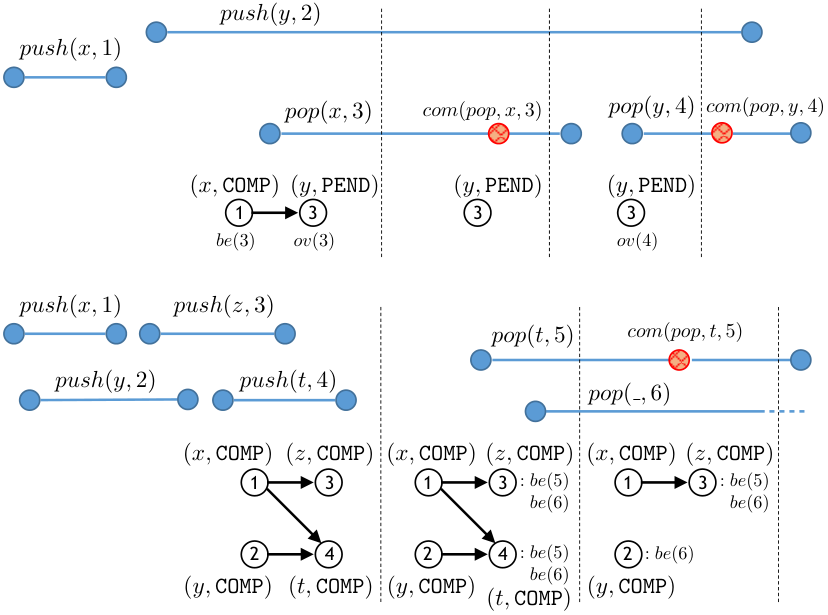
Figure 6 pictures two executions of $AbsS$ for two extended histories (that include pop commit points). For readability, we give the state of $AbsS$ only after several execution prefixes delimited at the right by a dotted line. We focus on pop operations – the effect of push calls and returns is similar to enqueue calls and returns in $AbsQ$. Let us first consider the history on the top part. The first state we give is reached after the call of pop with identifier $3$. This shows the effect of a pop invocation: the greatest completed pushes according to the current happens-before (here, the push with identifier $1$) are marked as $be(3)$ (from “before” operation 3), and the pending pushes are marked as $ov(3)$ (from “overlapping” with operation 3). As a side remark, any other push operation that starts after pop $3$ would be also marked as $ov(3)$. The commit point $com(pop,x,3)$ (pictured with a red circle) is enabled because $x$ was added by a push marked as $be(3)$. The effect of the commit point is that push $1$ is removed from the state (the execution on the bottom shows a more complicated case). For the second pop, the commit point $com(pop,y,4)$ is enabled because $y$ was added by a push marked as $ov(4)$. The execution on the bottom shows an example where the marking $be(k)$ for some pop $k$ is updated at commit points. The pushes $3$ and $4$ are marked as $be(5)$ and $be(6)$ when the pops $5$ and $6$ start. Then, $com(pop,t,5)$ is enabled since $t$ was added by $push(t,4)$ which is marked as $be(5)$. Besides removing $push(t,4)$, the commit point produces a state where a pop committing later, e.g., pop $6$, can remove $y$ which was added by a predecessor of $push(t,4)$ in the happens-before ($y$ could become the top of the stack when $t$ is removed). This history is valid because $push(y,2)$ can be linearized after $push(x,1)$ and $push(z,3)$. Thus, push 2, a predecessor of the push which is removed, is marked as $be(6)$. Push $1$ which is also a predecessor of the removed push is not marked as $be(6)$ because it happens before another push, i.e., push 3, which is already marked as $be(6)$ (the value added by push 3 should be removed before the value added by push 1 could become the top of the stack).

Formally, the states of $AbsS$ are tuples $\langle{O,<,\ell,rv,cp,be,ov}\rangle$ where $<$ is a strict partial order over the set $O$ of operation identifiers, $\ell:O\mathbin{\rightarrow}\mathchoice{\mbox{${\mathbb{V}}$}}{\mbox{${\mathbb{V}}$}}{\mbox{\scriptsize${\mathbb{V}}$}}{\mbox{\tiny${\mathbb{V}}$}}\times\{\tt{PEND,\tt{COMP}}\}$ labels every identifier in $O$ with a value and a pending/completed flag, $rv:\mathchoice{\mbox{${\mathbb{O}}$}}{\mbox{${\mathbb{O}}$}}{\mbox{\scriptsize${\mathbb{O}}$}}{\mbox{\tiny${\mathbb{O}}$}}{}\mathbin{\rightharpoonup}\mathchoice{\mbox{${\mathbb{V}}$}}{\mbox{${\mathbb{V}}$}}{\mbox{\scriptsize${\mathbb{V}}$}}{\mbox{\tiny${\mathbb{V}}$}}$ records the return value of a pending pop fixed at its commit point, $cp:\mathchoice{\mbox{${\mathbb{O}}$}}{\mbox{${\mathbb{O}}$}}{\mbox{\scriptsize${\mathbb{O}}$}}{\mbox{\tiny${\mathbb{O}}$}}{}\mathbin{\rightharpoonup}\{A_{1},A_{2},R_{1},R_{2},R_{3}\}$ records the control point of every push ($A_{1},A_{2}$) or pop operation ($R_{1},R_{2},R_{3}$), $be:\mathchoice{\mbox{${\mathbb{O}}$}}{\mbox{${\mathbb{O}}$}}{\mbox{\scriptsize${\mathbb{O}}$}}{\mbox{\tiny${\mathbb{O}}$}}{}\mathbin{\rightharpoonup}2^{O}$ records the greatest completed push operations before a pop started or happening earlier provided that the values of all the push happening later have been removed, and $ov:\mathchoice{\mbox{${\mathbb{O}}$}}{\mbox{${\mathbb{O}}$}}{\mbox{\scriptsize${\mathbb{O}}$}}{\mbox{\tiny${\mathbb{O}}$}}{}\mathbin{\rightharpoonup}2^{O}$ records push operations overlapping with a pop. All the components are $\emptyset$ in the initial state, and the transition relation $\mathbin{\rightarrow}$ is defined in Fig. 7.

The transition rules which don’t correspond to commit point actions are similar to those for $AbsQ$. The rule com-pop1 for $com(pop,d,k)$ is enabled only if there exists a push $k^{\prime}$ which added value $d$ and which belongs to $be(k)$ or $ov(k)$. When enabled, the push $k^{\prime}$ is removed from the set $O$ (and the order $<$) and for every other pop $k_{1}$ such that $k^{\prime}$ belongs to $be(k_{1})$, $k^{\prime}$ is replaced in $be(k_{1})$ by its predecessors which are followed exclusively by pushes overlapping with $k_{1}$ (these predecessors become maximal closed pushes once $k^{\prime}$ is removed). Also, $rv(k)$ is set to $d$. The rule com-pop1 for $com(pop,{\tt EMPTY},k)$ is enabled only if $be(k)$ is empty (i.e., all the values added by pushes ending before $k$, if any, have been removed). Then, $rv(k)$ is set to ${\tt EMPTY}$.

References

- [1] M. Abadi and L. Lamport. The existence of refinement mappings. Theor. Comput. Sci., 82(2):253–284, 1991. doi: 10.1016/0304-3975(91)90224-P. URL http://dx.doi.org/10.1016/0304-3975(91)90224-P.
- [2] P. A. Abdulla, F. Haziza, L. Holík, B. Jonsson, and A. Rezine. An integrated specification and verification technique for highly concurrent data structures. In TACAS, pages 324–338, 2013.
- [3] R. Alur, K. L. McMillan, and D. Peled. Model-checking of correctness conditions for concurrent objects. Inf. Comput., 160(1-2):167–188, 2000.
- [4] D. Amit, N. Rinetzky, T. W. Reps, M. Sagiv, and E. Yahav. Comparison under abstraction for verifying linearizability. In CAV ’07, volume 4590 of LNCS, pages 477–490, 2007.
- [5] A. Bouajjani, M. Emmi, C. Enea, and J. Hamza. Verifying concurrent programs against sequential specifications. In ESOP ’13, volume 7792 of LNCS, pages 290–309. Springer, 2013.
- [6] A. Bouajjani, M. Emmi, C. Enea, and J. Hamza. On reducing linearizability to state reachability. In M. M. Halldórsson, K. Iwama, N. Kobayashi, and B. Speckmann, editors, Automata, Languages, and Programming - 42nd International Colloquium, ICALP 2015, Kyoto, Japan, July 6-10, 2015, Proceedings, Part II, volume 9135 of Lecture Notes in Computer Science, pages 95–107. Springer, 2015a. ISBN 978-3-662-47665-9. doi: 10.1007/978-3-662-47666-6. URL http://dx.doi.org/10.1007/978-3-662-47666-6.
- [7] A. Bouajjani, M. Emmi, C. Enea, and J. Hamza. Tractable refinement checking for concurrent objects. In Rajamani and Walker [23], pages 651–662. ISBN 978-1-4503-3300-9. doi: 10.1145/2676726.2677002. URL http://doi.acm.org/10.1145/2676726.2677002.
- [8] J. Derrick, G. Schellhorn, and H. Wehrheim. Verifying Linearisability with Potential Linearisation Points, pages 323–337. Springer Berlin Heidelberg, Berlin, Heidelberg, 2011. ISBN 978-3-642-21437-0.
- [9] M. Dodds, A. Haas, and C. M. Kirsch. A scalable, correct time-stamped stack. In Rajamani and Walker [23], pages 233–246. ISBN 978-1-4503-3300-9. doi: 10.1145/2676726.2676963. URL http://doi.acm.org/10.1145/2676726.2676963.
- [10] C. Dragoi, A. Gupta, and T. A. Henzinger. Automatic linearizability proofs of concurrent objects with cooperating updates. In CAV ’13, volume 8044 of LNCS, pages 174–190. Springer.
- [11] I. Filipovic, P. W. O’Hearn, N. Rinetzky, and H. Yang. Abstraction for concurrent objects. Theor. Comput. Sci., 411(51-52):4379–4398, 2010.
- [12] M. Gorelik and D. Hendler. Brief announcement: an asymmetric flat-combining based queue algorithm. In P. Fatourou and G. Taubenfeld, editors, ACM Symposium on Principles of Distributed Computing, PODC ’13, Montreal, QC, Canada, July 22-24, 2013, pages 319–321. ACM, 2013. ISBN 978-1-4503-2065-8. doi: 10.1145/2484239.2484279. URL http://doi.acm.org/10.1145/2484239.2484279.
- [13] J. Hamza. On the complexity of linearizability. In A. Bouajjani and H. Fauconnier, editors, Networked Systems - Third International Conference, NETYS 2015, Agadir, Morocco, May 13-15, 2015, Revised Selected Papers, volume 9466 of Lecture Notes in Computer Science, pages 308–321. Springer, 2015. ISBN 978-3-319-26849-1. doi: 10.1007/978-3-319-26850-7. URL http://dx.doi.org/10.1007/978-3-319-26850-7.
- [14] D. Hendler, N. Shavit, and L. Yerushalmi. A scalable lock-free stack algorithm. In SPAA 2004, pages 206–215. ACM.
- [15] D. Hendler, I. Incze, N. Shavit, and M. Tzafrir. Flat combining and the synchronization-parallelism tradeoff. In F. M. auf der Heide and C. A. Phillips, editors, SPAA 2010: Proceedings of the 22nd Annual ACM Symposium on Parallelism in Algorithms and Architectures, Thira, Santorini, Greece, June 13-15, 2010, pages 355–364. ACM, 2010. ISBN 978-1-4503-0079-7. doi: 10.1145/1810479.1810540. URL http://doi.acm.org/10.1145/1810479.1810540.
- [16] T. A. Henzinger, A. Sezgin, and V. Vafeiadis. Aspect-oriented linearizability proofs. In CONCUR, pages 242–256, 2013.
- [17] M. Herlihy and J. M. Wing. Linearizability: A correctness condition for concurrent objects. ACM Trans. Program. Lang. Syst., 12(3):463–492, 1990.
- [18] M. Hoffman, O. Shalev, and N. Shavit. The baskets queue. In E. Tovar, P. Tsigas, and H. Fouchal, editors, Principles of Distributed Systems, 11th International Conference, OPODIS 2007, Guadeloupe, French West Indies, December 17-20, 2007. Proceedings, volume 4878 of Lecture Notes in Computer Science, pages 401–414. Springer, 2007. ISBN 978-3-540-77095-4.
- [19] H. Liang and X. Feng. Modular verification of linearizability with non-fixed linearization points. In H. Boehm and C. Flanagan, editors, ACM SIGPLAN Conference on Programming Language Design and Implementation, PLDI ’13, Seattle, WA, USA, June 16-19, 2013, pages 459–470. ACM, 2013. ISBN 978-1-4503-2014-6. doi: 10.1145/2462156.2462189. URL http://doi.acm.org/10.1145/2462156.2462189.
- [20] N. A. Lynch and F. W. Vaandrager. Forward and backward simulations: I. untimed systems. Inf. Comput., 121(2):214–233, 1995. doi: 10.1006/inco.1995.1134. URL http://dx.doi.org/10.1006/inco.1995.1134.
- [21] A. Morrison and Y. Afek. Fast concurrent queues for x86 processors. In A. Nicolau, X. Shen, S. P. Amarasinghe, and R. W. Vuduc, editors, ACM SIGPLAN Symposium on Principles and Practice of Parallel Programming, PPoPP ’13, Shenzhen, China, February 23-27, 2013, pages 103–112. ACM, 2013. ISBN 978-1-4503-1922-5. doi: 10.1145/2442516.2442527. URL http://doi.acm.org/10.1145/2442516.2442527.
- [22] P. W. O’Hearn, N. Rinetzky, M. T. Vechev, E. Yahav, and G. Yorsh. Verifying linearizability with hindsight. In PODC ’10, pages 85–94. ACM.
- [23] S. K. Rajamani and D. Walker, editors. Proceedings of the 42nd Annual ACM SIGPLAN-SIGACT Symposium on Principles of Programming Languages, POPL 2015, Mumbai, India, January 15-17, 2015, 2015. ACM. ISBN 978-1-4503-3300-9. URL http://dl.acm.org/citation.cfm?id=2676726.
- [24] G. Schellhorn, H. Wehrheim, and J. Derrick. How to prove algorithms linearisable. In P. Madhusudan and S. A. Seshia, editors, Computer Aided Verification - 24th International Conference, CAV 2012, Berkeley, CA, USA, July 7-13, 2012 Proceedings, volume 7358 of Lecture Notes in Computer Science, pages 243–259. Springer, 2012. ISBN 978-3-642-31423-0. doi: 10.1007/978-3-642-31424-7. URL http://dx.doi.org/10.1007/978-3-642-31424-7.
- [25] V. Vafeiadis. Automatically proving linearizability. In CAV ’10, volume 6174 of LNCS, pages 450–464.
- [26] V. Vafeiadis. Modular fine-grained concurrency verification. PhD thesis, University of Cambridge, 2008.
- [27] V. Vafeiadis. Shape-value abstraction for verifying linearizability. In VMCAI ’09: Proc. 10th Intl. Conf. on Verification, Model Checking, and Abstract Interpretation, volume 5403 of LNCS, pages 335–348. Springer, 2009.
- [28] V. Vafeiadis, M. Herlihy, T. Hoare, and M. Shapiro. Proving correctness of highly-concurrent linearisable objects. In PPOPP ’06, pages 129–136. ACM.
- [29] H. Zhu, G. Petri, and S. Jagannathan. Poling: SMT aided linearizability proofs. In D. Kroening and C. S. Pasareanu, editors, Computer Aided Verification - 27th International Conference, CAV 2015, San Francisco, CA, USA, July 18-24, 2015, Proceedings, Part II, volume 9207 of Lecture Notes in Computer Science, pages 3–19. Springer, 2015. ISBN 978-3-319-21667-6. doi: 10.1007/978-3-319-21668-3. URL http://dx.doi.org/10.1007/978-3-319-21668-3.
Appendix 0.A Libraries