跳到论文正文
W Papers独立论文阅读器 arXiv:1702.02701 论文正文 计算阅读时间 · 0%
引用这篇论文根据当前论文元数据生成,正式投稿前建议核对。


License: arXiv.org perpetual non-exclusive license
arXiv:1702.02701v2 [math.NA] 13 Jun 2018

A Posteriori Error Estimation and Adaptive Algorithm for Atomistic/Continuum Coupling in 2DThanks: Submitted to the editors on August 24, 2026.

Hao Wang ††thanks: College of Mathematics, Sichuan University, No.24 South Section One, Yihuan Road, Chengdu, 610065, China (). Email: wangh@scu.edu.cn    Mingjie Liao ††thanks: Department of Applied Mathematics and Mechanics, University of Science and Technology Beijing, No. 30 Xueyuan Road, Haidian District, Beijing 100083 (). Email: mliao@xs.ustb.edu.cn    Ping Lin ††thanks: Department of Mathematics, University of Dundee, Dundee, DD1 4HN, Scotland, United Kingdom (). Email: plin@maths.dundee.ac.uk    Lei Zhang ††thanks: Institute of Natural Sciences, School of Mathematical Sciences, and Ministry of Education Key Laboratory of Scientific and Engineering Computing (MOE-LSC), Shanghai Jiao Tong University, 800 Dongchuan Road, Shanghai 200240, China (). Email: lzhang2012@sjtu.edu.cn
Abstract

Atomistic/continuum coupling methods aim to achieve optimal balance between accuracy and efficiency. Adaptivity is the key for the efficient implementation of such methods. In this paper, we carry out a rigorous a posteriori analysis of the residual, the stability constant, and the error bound, for a consistent atomistic/continuum coupling method in 2D. We design and implement the corresponding adaptive mesh refinement algorithm, and the convergence rate with respect to degrees of freedom is optimal compare with a priori error estimates.

keywords
atomistic models, coarse graining, atomistic-to-continuum coupling, adaptive algorithm, a posteriori error estimate
Funding.
HW was partially supported by NSFC grant 11501389, 11471214 and Sichuan University Starting Up Research Funding No. 2082204194117. PL and ML were partially supported by NSFC grant 91430106 and Fundamental Research Funds for Central Universities Nos. 06108038 and FRF-BR-13-023. PL and HW were partially supported by EMS RSF grant. LZ was partially supported by NSFC grant 11471214, 11571314 and the One Thousand Plan of China for young scientists.
††runningheads: A Posteriori Estimation A/C Coupling 2D / H. Wang, M.Liao, P.Lin and L. Zhang
AMS
65N12, 65N15, 70C20, 82D25

1 Introduction

Atomistic/continuum (a/c) coupling methods are a class of computational multiscale methods that aim to combine the accuracy of the atomistic model and the efficiency of the continuum model for crystalline solids with defects [26, 43, 14]. Namely, the atomistic model can be applied in a small neighborhood of the localized defects such as vacancies, dislocations, and cracks, while the continuum model (e.g., Cauchy-Born rule) can be employed away from the defect cores where elastic deformation occurs. The construction and analysis of different a/c coupling methods have attracted considerable attention in the research community in recent years [16, 31, 19, 18]. We refer the readers to [23, 20] for a review of such methods.

The goal of the mathematical analysis for a/c coupling methods is to find the optimal relation of accuracy vs. degrees of freedom. The a priori analysis has been carried out for several typical a/c coupling methods, for example the QNL (quasi-nonlocal quasicontinuum) method [24, 34], the BQCE (blended energy-based quasi-continuum) method [15], the BQCF (blended force-based quasi-continuum) method [18, 15], the GRAC (geometric reconstruction based atomistic/continuum coupling) method [36] and the BGFC (atomistic/continuum blending with ghost force correction) method [38].

In contrast, although adaptivity is the key for the efficient implementation of a/c coupling methods, only few research articles are concerned with the a posteriori error control of these methods. The goal-oriented approach has been utilised in [40] by Prudhomme et al. to provide a posteriori error control for a three dimensional nanoindentation problem with the quantity of interest being the force acting on the indenter. The error estimator is a modification of the rigorously derived residual functional, and its effectiveness is only validated numerically. Arndt and Luskin [2, 3] analyze the goal-oriented approach for a one dimensional Frenkel-Kontorova model, where the a posteriori error estimators are used to optimize the choice of the atomistic region as well as the finite element mesh in the continuum region. All these work employ the original energy-based quasicontinuum method as the underlying model which is later shown to be inconsistent and suffers from the so-called ”ghost force” [43, 7, 17, 24, 22]. Recently, Kochmann et al. [47] proposed an adaptivity strategy for the so-call ”fully-nonlocal quasi-continuum” method which apply a discrete model in the entire computational domain without coupling of different models. This approach aims to minimize the ghost force rather than eliminate it as in the consistent a/c coupling method.

The residual based a posteriori error bounds for a/c coupling schemes are first derived in [32, 27] by Ortner et al. in 1D. A recent advance in this direction [35] is the a posteriori error analysis of a consistent energy-based coupling method developed in [41, 42], where the a posteriori error estimators are proposed both in the energy norm and in energy itself. For complex lattice, a posteriori error analysis for the QC method in 1D has been carried out in [1].

Despite all those developments, the rigorous mathematical justification of a posteriori error estimates beyond 1D is still missing. In this paper, we present a rigorous a posteriori error estimate for a consistent energy-based a/c method in two dimension, which is of physical significance and has not been considered so far to the best knowledge of the authors. We use the residual-based approach [48] to establish the estimate in negative Sobolev norms following [35]. Two features distinguish our problem from the classic residual-based estimate for finite element approximation of the elliptic equations. The first one is the existence of the modeling error which is in origin different from the applications of quadrature rules. The second one is that the mesh may not be further refined when it almost coincides with the reference lattice, therefore a model adaptation should be imposed. The analysis and algorithm rely on the so-called divergence free tensor field, which characterizes the essential difference of 2D results compared with 1D results in [27, 35] where the analysis can be carried out by explicit calculations.

Similar to the a priori analysis of GRAC in [36], we constrain ourselves to the case of nearest-neighbor interactions. Although the analysis can be extended to finite range interactions and to other a/c coupling methods, we decide not to include these so that the main ideas and steps are clearly presented without the distraction from the unnecessary complexity of the presentation. Instead, we will make further remarks on this point again in § 5.

The paper is organized as follows. In § 2 we set up the atomistic, continuum and coupling models for point defects. In § 3 we present the main results: the residual estimate, stability bound, and rigorous a posteriori error estimates for the coupling scheme. We formulate the corresponding adaptive algorithm and demonstrate numerical results in § 4. We draw conclusions and make suggestions for future research in § 5. Some auxiliary results are given in § Appendix A.

2 Formulation

We first give a brief review of a model for crystal defects in an infinite lattice in the spirit of [11] in § 2.1 and the Cauchy-Born continuum model in § 2.2. We then present a generic form of a/c coupling schemes in § 2.3. We will introduce the consistent scheme GRAC specifically in § 2.4.

2.1 Atomistic model

2.1.1 Atomistic lattice and defects

Given d∈{2,3}d\in\{2,3\}, 𝖠∈ℝd×d{\sf A}\in\mathbb{R}^{d\times d} non-singular, Λhom:=𝖠​ℤd\Lambda^{\rm hom}:={\sf A}\mathbb{Z}^{d} is the homogeneous reference lattice which represents a perfect single lattice crystal formed by identical atoms and possessing no defects. Λ⊂ℝd\Lambda\subset\mathbb{R}^{d} is the reference lattice with some local defects. The mismatch between Λ\Lambda and Λhom\Lambda^{\rm hom} represents possible defects Λdef\Lambda^{\rm def}, which are contained in some localized defect cores DdefD^{\rm def} such that the atoms in Λ∖Ddef\Lambda\setminus D^{\rm def} do not interact with defects Λdef\Lambda^{\rm def} (see § 2.1.2 and § 2.1.3 regarding interaction neighbourhood). For example, Λdef={x}\Lambda^{\rm def}=\{x\} for a crystal with a single point defect at xx, and one can choose a proper radius Rdef>0R^{\rm def}>0 such that Ddef=Bx,RdefD^{\rm def}=B_{x,R^{\rm def}}, where Bx,R:={z∈ℝd||z−x|≤R}B_{x,R}:=\{z\in\mathbb{R}^{d}\,|\,|z-x|\leq R\}. For different types of point defects, we have

  • •

    Λ⊂Λhom\Lambda\subset\Lambda^{\rm hom} for a vacancy at x∈Λhomx\in\Lambda^{\rm hom};

  • •

    Λ⊃Λhom\Lambda\supset\Lambda^{\rm hom} for an interstitial at x∈Λx\in\Lambda but x∉Λhomx\notin\Lambda^{\rm hom};

  • •

    Λ=Λhom\Lambda=\Lambda^{\rm hom} for an impurity at x∈Λhomx\in\Lambda^{\rm hom}, the difference of the impurity atom with other atoms can be characterized by the inhomogeneity of interaction potentials (see § 2.1.3).

This characterization of localized defects can be straightforwardly generalized to multiple point defects and micro-cracks, for example, see the setup of the model problem in § 4.2. Straight screw dislocations can be enforced through the appropriate choice of boundary conditions [11].

2.1.2 Lattice function and lattice function space

Given d∈{2,3}d\in\{2,3\}, m∈{1,2,3}m\in\{1,2,3\}, denote the set of vector-valued lattice functions by

𝒰:={v:Λ→ℝm}.\mathscr{U}:=\{v:\Lambda\to\mathbb{R}^{m}\}.

A deformed configuration is a lattice function y∈𝒰y\in\mathscr{U}. Let xx be the identity map, the displacement u∈𝒰u\in\mathscr{U} is defined by u⁡(ℓ)=y⁡(ℓ)−x⁡(ℓ)=y⁡(ℓ)−ℓu(\ell)=y(\ell)-x(\ell)=y(\ell)-\ell for any ℓ∈Λ\ell\in\Lambda.

For each ℓ∈Λ\ell\in\Lambda, we prescribe an interaction neighbourhood 𝒩ℓ:={ℓ′∈Λ| 0<|ℓ′−ℓ|≤rcut}\mathcal{N}_{\ell}:=\{\ell^{\prime}\in\Lambda\,|\,0<|\ell^{\prime}-\ell|\leq r_{\rm cut}\} with some cut-off radius rcutr_{\rm cut}. The interaction range ℛℓ:={ℓ′−ℓ|ℓ′∈𝒩ℓ}\mathcal{R}_{\ell}:=\{\ell^{\prime}-\ell\,|\,\ell^{\prime}\in\mathcal{N}_{\ell}\} is defined as the union of lattice vectors defined by the finite difference of lattice points in 𝒩ℓ\mathcal{N}_{\ell} and ℓ\ell.

To measure the error for lattice functions we need to introduce function norms and function spaces on the lattice. Define the “finite difference stencil” D​v​(ℓ):={Dρ​v​(ℓ)}ρ∈ℛℓ:={v⁡(ℓ+ρ)−v⁡(ℓ)}ρ∈ℛℓDv(\ell):=\{D_{\rho}v(\ell)\}_{\rho\in\mathcal{R}_{\ell}}:=\{v(\ell+\rho)-v(\ell)\}_{\rho\in\mathcal{R}_{\ell}}. Higher-order finite differences, e.g., Dρ​Dς​vD_{\rho}D_{\varsigma}v and D2​vD^{2}v can be defined in a canonical way. A lattice function norm can hence be defined using those notations. For v∈𝒰v\in\mathscr{U}, let the lattice energy-norm (a discrete H1H^{1}-semi-norm) be

‖D​v‖ℓ2:=(∑ℓ∈Λ∑ρ∈ℛℓ|Dρ​v​(ℓ)|2)1/2.\|Dv\|_{\ell^{2}}:=\bigg(\sum_{\ell\in\Lambda}\sum_{\rho\in\mathcal{R}_{\ell}}|D_{\rho}v(\ell)|^{2}\bigg)^{1/2}. (1)

The associated lattice function space is defined by

𝒰˙1,2\displaystyle\dot{\mathscr{U}}^{1,2} :={u:Λ→ℝm|∥Du∥ℓ2<+∞}.\displaystyle:=\big\{u:\Lambda\to\mathbb{R}^{m}\,\big|\,\|Du\|_{\ell^{2}}<+\infty\big\}.

We choose

ℬ:={(ℓ,ℓ+ρ):ℓ∈Λ,ρ∈ℛℓ}\mathcal{B}:=\{(\ell,\ell+\rho):\ell\in\Lambda,\rho\in\mathcal{R}_{\ell}\} (2)

to be the collection of all the nearest neighbour bonds in the reference lattice, and for b=(ℓ,ℓ+ρ)∈ℬb=(\ell,\ell+\rho)\in\mathcal{B}, denote ρb=ρ\rho_{b}=\rho. Then the energy norm can be reformulated as

‖D​v‖ℓ2:=(∑b=(ℓ,ℓ+ρ)∈ℬ|Dρ​v​(ℓ)|2)1/2.\|Dv\|_{\ell^{2}}:=\bigg(\sum_{b=(\ell,\ell+\rho)\in\mathcal{B}}|D_{\rho}v(\ell)|^{2}\bigg)^{1/2}. (3)

The homogeneous lattice Λhom=𝖠​ℤd\Lambda^{\rm hom}={\sf A}\mathbb{Z}^{d} naturally induces a simplicial micro-triangulation 𝒯\mathcal{T}. In 2D, 𝒯a={𝖠ξ+T^,𝖠ξ−T^|ξ∈ℤ2}\mathcal{T}^{{\rm a}}=\{{\sf A}\xi+\hat{T},{\sf A}\xi-\hat{T}|\xi\in\mathbb{Z}^{2}\}, where T^=conv⁡{0,e1,e2}\hat{T}={\rm conv}\{0,e_{1},e_{2}\}. Let ζ¯∈W1,∞​(Λhom,ℝ)\bar{\zeta}\in W^{1,\infty}(\Lambda^{\rm hom};\mathbb{R}) be the P1 nodal basis function associated with the origin; namely, ζ¯\bar{\zeta} is piecewise linear with respect to 𝒯a\mathcal{T}^{\rm a}, and ζ¯​(0)=1\bar{\zeta}(0)=1 and ζ¯​(ξ)=0\bar{\zeta}(\xi)=0 for ξ≠0\xi\neq 0 and ξ∈Λhom\xi\in\Lambda^{\rm hom}. The nodal interpolant of v∈𝒰v\in\mathscr{U} can be written as

v¯​(x):=∑ξ∈ℤdv⁡(ξ)​ζ¯​(x−ξ).\bar{v}(x):=\sum_{\xi\in\mathbb{Z}^{d}}v(\xi)\bar{\zeta}(x-\xi).

We can introduce the discrete homogeneous Sobolev spaces

𝒰1,2:={u∈𝒰|∇u¯∈L2},\mathscr{U}^{1,2}:=\{u\in\mathscr{U}|\nabla\bar{u}\in L^{2}\},

with semi-norm ‖∇u¯‖L2\|\nabla\bar{u}\|_{L^{2}}. It is known from [30] that 𝒰˙1,2\dot{\mathscr{U}}^{1,2} and 𝒰1,2\mathscr{U}^{1,2} are equivalent.

2.1.3 Interaction potential

For each ℓ∈Λ\ell\in\Lambda, let Vℓ​(y)V_{\ell}(y) denote the site energy associated with the lattice site ℓ∈Λ\ell\in\Lambda, and we assume that Vℓ​(y)∈Ck​((ℝd)ℛℓ),k≥2V_{\ell}(y)\in C^{k}((\mathbb{R}^{d})^{\mathcal{R}_{\ell}}),k\geq 2. In this paper, we consider the general multibody interaction potential of the generic pair functional form [46]. Namely, the potential is a function of the distances between atoms within interaction range and with no angular dependence. Accordingly, we have the following equivalent forms of interaction potentials of generic pair functional form,

Vℓ​(y)=V^ℓ​({Dρ​y​(ℓ)}ρ∈ℛℓ)=V~ℓ​({|Dρ​y​(ℓ)|}ρ∈ℛℓ)V_{\ell}(y)=\widehat{V}_{\ell}(\{D_{\rho}y(\ell)\}_{\rho\in\mathcal{R}_{\ell}})=\widetilde{V}_{\ell}(\{|D_{\rho}y(\ell)|\}_{\rho\in\mathcal{R}_{\ell}}) (4)
Remark 2.1.

For convenience, with a slight abuse of notation, we will use Vℓ​(Dρ​y)V_{\ell}(D_{\rho}y), Vℓ​(|Dρ​y|)V_{\ell}(|D_{\rho}y|) instead of V^ℓ​({Dρ​y​(ℓ)}ρ∈ℛℓ)\widehat{V}_{\ell}(\{D_{\rho}y(\ell)\}_{\rho\in\mathcal{R}_{\ell}}), V~ℓ​({|Dρ​y​(ℓ)|}ρ∈ℛℓ)\widetilde{V}_{\ell}(\{|D_{\rho}y(\ell)|\}_{\rho\in\mathcal{R}_{\ell}}) when there is no confusion in the context.

We assume that VℓV_{\ell} is homogeneous outside the defect region DdefD^{\rm def}, namely, Vℓ=VV_{\ell}=V and ℛℓ=ℛ\mathcal{R}_{\ell}=\mathcal{R} for ℓ∈Λ∖Ddef\ell\in\Lambda\setminus D^{\rm def}. VV and ℛ\mathcal{R} have the following point symmetry: ℛ=−ℛ\mathcal{R}=-\mathcal{R}, and V⁡({−g−ρ}ρ∈ℛ)=V⁡(g)V(\{-g_{-\rho}\}_{\rho\in\mathcal{R}})=V(g).

Remark 2.2.

Notice that both displacement uu and deformation yy are discrete functions belonging to 𝒰\mathscr{U}, however u∈𝒰˙1,2u\in\dot{\mathscr{U}}^{1,2} while y∉𝒰˙1,2y\notin\dot{\mathscr{U}}^{1,2}. We define the interaction potential VV through yy for the convenience of stability analysis, the consistency results are the same either with uu or with yy.

A great number of practical potentials are in the form (4), including the widely used embedded atom model (EAM) [6] and Finnis-Sinclair model [13]. For example, assuming a finite interaction neighborhood 𝒩ℓ\mathcal{N}_{\ell} and an interaction range ℛℓ\mathcal{R}_{\ell} for ℓ∈Λ\ell\in\Lambda, EAM potential reads

Vℓ​(y):=\displaystyle V_{\ell}(y):= ∑ℓ′∈𝒩ℓϕ⁡(|y⁡(ℓ)−y⁡(ℓ′)|)+F⁡(∑ℓ′∈𝒩ℓψ⁡(|y⁡(ℓ)−y⁡(ℓ′)|)),\displaystyle\sum_{\ell^{\prime}\in\mathcal{N}_{\ell}}\phi(|y(\ell)-y(\ell^{\prime})|)+F\Big({\textstyle\sum_{\ell^{\prime}\in\mathcal{N}_{\ell}}\psi(|y(\ell)-y(\ell^{\prime})|)}\Big),
=\displaystyle= ∑ρ∈ℛℓϕ⁡(|Dρ​y​(ℓ)|)+F⁡(∑ρ∈ℛℓψ⁡(|Dρ​y​(ℓ)|)).\displaystyle\sum_{\rho\in\mathcal{R}_{\ell}}\phi\big(|D_{\rho}y(\ell)|\big)+F\Big({\textstyle\sum_{\rho\in\mathcal{R}_{\ell}}}\psi\big(|D_{\rho}y(\ell)|\big)\Big). (5)

for a pair potential ϕ\phi, an electron density function ψ\psi and an embedding function FF.

The energy of an infinite configuration is typically ill-defined. However, if we redefine the potential Vℓ​(y)V_{\ell}(y) as the difference Vℓ​(y)−Vℓ​(ℓ)V_{\ell}(y)-V_{\ell}(\ell), which is equivalent to assuming Vℓ​(ℓ)=0V_{\ell}(\ell)=0, the energy functional

ℰa​(y)=∑ℓ∈ΛVℓ​(y)\mathscr{E}^{\rm a}(y)=\sum_{\ell\in\Lambda}V_{\ell}(y) (6)

is a meaningful object. Given the point symmetry and smoothness assumptions for the site potentials VℓV_{\ell}, ℰa​(y)\mathscr{E}^{\rm a}(y) is well-defined for y−yB∈𝒰1,2y-y^{B}\in\mathscr{U}^{1,2}, where yB​(x)=B​xy^{B}(x)=Bx. Furthermore, if Vℓ​(y)V_{\ell}(y) is CkC^{k} in its variables, ℰa\mathscr{E}^{\rm a} is kk times Fréchet differentiable. In particular, we define MM as the Lipschitz constant of δ2​ℰa\delta^{2}\mathscr{E}^{\rm a}, by [11, Lemma 2.1].

Under the above conditions, the goal of the atomistic problem is to find a strongly stable equilibrium yy, such that, given a macroscopic applied strain B∈ℝd×dB\in\mathbb{R}^{d\times d}, we aim to compute

y∈arg⁡min⁡{ℰa​(y)|y−yB∈𝒰1,2}.y\in\arg\min\big\{\mathscr{E}^{\rm a}(y)\,\big|\,y-y^{B}\in\mathscr{U}^{1,2}\big\}. (7)

yy is strongly stable if there exists c0>0c_{0}>0 such that

⟨δ2​ℰa​(y)​v,v⟩≥c0​‖∇v‖L22,∀v∈𝒰1,2.\langle\delta^{2}\mathscr{E}^{\rm a}(y)v,v\rangle\geq c_{0}\|\nabla v\|_{L^{2}}^{2},\quad\forall v\in\mathscr{U}^{1,2}.

.

It is proven in [11, Theorem 2.3 ] that, if the homogeneous lattice is stable and y∈𝒰y\in\mathscr{U} is a critical point of ℰa\mathscr{E}^{\rm a} such that u=y−yB∈𝒰1,2u=y-y^{B}\in\mathscr{U}^{1,2}, then Dj​uD^{j}u exhibit the following generic decay, j=0,1,…j=0,1,\dots,

|Dj​u​(ℓ)|≲|ℓ|1−d−j,and|u⁡(ℓ)−u∞|≲|ℓ|−d+1.\big|D^{j}u(\ell)\big|\lesssim|\ell|^{1-d-j},\quad\text{and}\quad\big|u(\ell)-u_{\infty}\big|\lesssim|\ell|^{-d+1}. (8)

where u∞:=lim|ℓ|→∞u⁡(ℓ)u_{\infty}:=\lim_{|\ell|\to\infty}u(\ell).

2.2 Continuum model

To formulate atomistic to continuum coupling schemes, we need a continuum model which is compatible with (6) and defined through a strain energy density function W:ℝd×d→ℝW:\mathbb{R}^{d\times d}\to\mathbb{R}. Let VV be the homogeneous site potential on Λhom\Lambda^{\rm hom}. A typical choice in the multi-scale context is the Cauchy–Born continuum model [10, 33], the energy density WW is defined by

W⁡(𝖥):=det𝖠−1​V​(𝖥​x).W({\sf F}):=\det{\sf A}^{-1}V({\sf F}x).

2.3 A/C coupling

We give a generic formulation of the a/c coupling method and employ concepts and notation from various earlier works, such as [26, 43, 44, 21, 37], and we adapt the formulation to the settings in this paper.

First, the computational domain ΩR⊂ℝd\Omega_{R}\subset\mathbb{R}^{d} is a simply connected, polygonal and closed set, such that B0,R⊂ΩR⊂B0,c0​RB_{0,R}\subset\Omega_{R}\subset B_{0,c_{0}R} for some c0>0c_{0}>0. Let RR be the radius of ΩR\Omega_{R} We have the following decomposition ΩR=ΩRa​⋃ΩRc\Omega_{R}=\Omega_{R}^{\rm a}\bigcup\Omega_{R}^{\rm c}, where the atomistic region ΩRa\Omega^{\rm a}_{R} is again simply connected and polygonal, and contains the defect core: Ddef⊂ΩRaD^{\rm def}\subset\Omega^{\rm a}_{R}. Let RaR_{\rm a} be the radius of ΩRa\Omega^{\rm a}_{R}. Let 𝒯h,Rc\mathcal{T}^{c}_{h,R} be a shape-regular simplicial partition (triangles for d=2d=2 or tetrahedra for d=3d=3) of the continuum region ΩRc\Omega^{\rm c}_{R}.

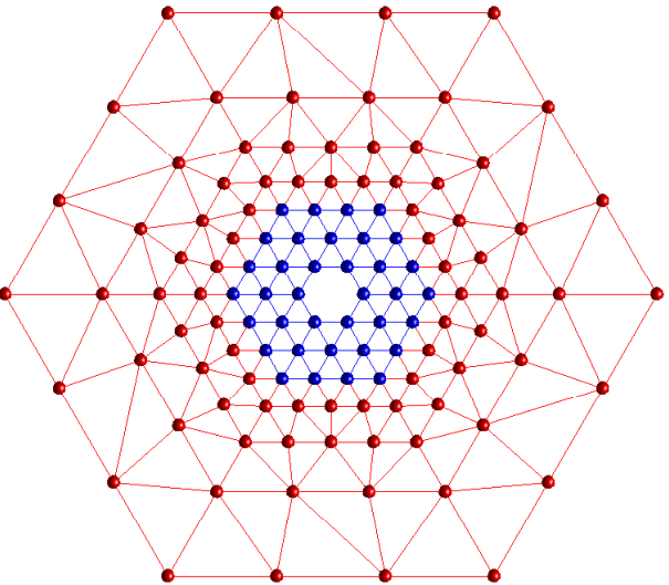
Next, we decompose the set of atoms Λa,i:=Λ​⋂ΩRa=Λa​⋃Λi\Lambda^{{\rm a},{\rm i}}:=\Lambda\bigcap\Omega^{\rm a}_{R}=\Lambda^{\rm a}\bigcup\Lambda^{\rm i} into a core atomistic set Λa\Lambda^{\rm a} and an interface set Λi\Lambda^{\rm i} (typically a few “layers” of atoms surrounding Λa\Lambda^{\rm a}) such that Λ​⋂Ddef⊂Λa\Lambda\bigcap D^{\rm def}\subset\Lambda^{\rm a}. Let 𝒯h,Ra\mathcal{T}^{\rm a}_{h,R} be the canonical triangulation induced by Λa,i\Lambda^{{\rm a},{\rm i}}, which may contain ”holes” due to the existence of defects, and 𝒯h,R=𝒯h,Rc​⋃𝒯h,Ra{\mathcal{T}_{h,R}}=\mathcal{T}^{\rm c}_{h,R}\bigcup\mathcal{T}^{\rm a}_{h,R}. Sometimes, it is also convenient to define 𝒯h,Ri:={T∈𝒯h,R:Λi​⋂T≠∅}\mathcal{T}^{\rm i}_{h,R}:=\{T\in{\mathcal{T}_{h,R}}:\Lambda^{{\rm i}}\bigcap T\neq\emptyset\}. Please see Figure 1 for an illustration of the computational mesh.
Refer to caption
Figure 1: Illustration of computational mesh. The computational domain is ΩR\Omega_{R}, and the corresponding triangulation is 𝒯h,R\mathcal{T}_{h,R}. Blue nodes in ΩR\Omega_{R} are atoms in Λa,i\Lambda^{{\rm a},{\rm i}}. For nearest neighbour interaction, Λi\Lambda^{\rm i} is the set of outmost layer of blue atoms. Red nodes in 𝒯h,R\mathcal{T}_{h,R} are continuum degrees of freedom. ΩRa\Omega_{R}^{\rm a} is the domain induced by the blue nodes, and 𝒯h,Ra\mathcal{T}^{\rm a}_{h,R} is the corresponding triangulation. ΩRc\Omega_{R}^{c} and 𝒯h,Rc\mathcal{T}^{\rm c}_{h,R} are the respective complements of ΩRa\Omega_{R}^{\rm a} and 𝒯h,R\mathcal{T}_{h,R}.

Let Ωh,R=⋃T∈𝒯h,RT\Omega_{h,R}=\bigcup_{T\in{\mathcal{T}_{h,R}}}T. Notice that Ωh,R\Omega_{h,R} can be multiple-connected, and ΩR∖Ωh,R\Omega_{R}\setminus\Omega_{h,R} characterizes possible defects. The space of coarse-grained displacements is,

𝒰h,R:={uh:Ωh,R→ℝm|\displaystyle\mathscr{U}_{h,R}:=\big\{u_{h}:\Omega_{h,R}\to\mathbb{R}^{m}\,\big|\,~ uhu_{h} is continuous and p.w. affine w.r.t. 𝒯h,R\mathcal{T}_{h,R},
uh=0 on ∂ΩR }.\displaystyle\text{ $u_{h}=0$ on $\partial\Omega_{R}$ }\big\}.

We may drop the subscript RR in the above definitions, for example, use 𝒯h\mathcal{T}_{h} instead of 𝒯h,R{\mathcal{T}_{h,R}} if there is no confusion. Let 𝒩h\mathcal{N}_{h} be the set of nodes in 𝒯h\mathcal{T}_{h}, and ℱh\mathcal{F}_{h} be the set of edges in 𝒯h\mathcal{T}_{h}.

Denote vor⁡(ℓ)\rm vor(\ell) as the voronoi cell associated with atom ℓ\ell, the volume of this cell denoted as |vor⁡(ℓ)||\rm vor(\ell)| equals the volume of the unit cell in Λhom\Lambda^{\rm hom}, i.e. vor⁡(ℓ)=det(𝖠)\rm vor(\ell)=\det({\sf A}). For each ℓ∈Λa\ell\in\Lambda^{{\rm a}}, the associated effective volume is vℓ=vor⁡(ℓ)v_{\ell}=\rm vor(\ell). For ℓ∈Λi\ell\in\Lambda^{\rm i} the effective volume vℓv_{\ell} will depend on the geometry of the interface (see [36]), let ωℓ:=|vℓ||vor⁡(ℓ)|\omega_{\ell}:=\displaystyle{\frac{|v_{\ell}|}{|{\rm vor}(\ell)|}} denote the volume ratio of vℓv_{\ell} with respect to vor\rm vor. For each element T∈𝒯hT\in\mathcal{T}_{h} we define the effective volume of TT by

ωT:=|T∖(⋃ℓ∈Λavor⁡(ℓ))∖(⋃ℓ∈Λivℓi)|.\omega_{T}:=|T\setminus(\bigcup_{\ell\in\Lambda^{{\rm a}}}{\rm vor}(\ell))\setminus(\bigcup_{\ell\in\Lambda^{{\rm i}}}v^{\rm i}_{\ell})|.

We note that ωT=0\omega_{T}=0 if T∈𝒯ha∖𝒯hiT\in\mathcal{T}^{\rm a}_{h}\setminus\mathcal{T}^{\rm i}_{h}, ωT=|T|\omega_{T}=|T| if T∈𝒯hc∖𝒯hiT\in\mathcal{T}^{\rm c}_{h}\setminus\mathcal{T}^{\rm i}_{h}, and 0≤ωT<|T|0\leq\omega_{T}<|T| if T∈𝒯hiT\in\mathcal{T}^{\rm i}_{h}. The choices of vℓv_{\ell} and ωT\omega_{T} satisfy ∑ℓ∈Λa,ivℓ+∑T∈𝒯hωT=|Ωh,R|\sum_{\ell\in\Lambda^{{\rm a},{\rm i}}}v_{\ell}+\sum_{T\in\mathcal{T}_{h}}\omega_{T}=|\Omega_{h,R}|.

Now we are ready to define the generic a/c coupling energy functional ℰh\mathscr{E}^{\rm h},

ℰh​(yh):=\displaystyle\mathscr{E}^{\rm h}(y_{h}):= ∑ℓ∈ΛaVℓ​(yh)+∑ℓ∈Λiωℓ​Vℓi​(yh)+∑T∈𝒯hωT​W​(∇yh|T)\displaystyle\sum_{\ell\in\Lambda^{\rm a}}V_{\ell}(y_{h})+\sum_{\ell\in\Lambda^{\rm i}}\omega_{\ell}V^{\rm i}_{\ell}(y_{h})+\sum_{T\in\mathcal{T}_{h}}\omega_{T}W(\nabla y_{h}|_{T}) (9)

where VℓiV_{\ell}^{\rm i} is a modified interface site potential which satisfies consistency conditions (11) and (12). ωℓ\omega_{\ell} and ωT\omega_{T} are suitable coefficients, and their construction will be discussed immediately in Section § 2.4 and references therein.

The goal of a/c coupling is to find

yh,R∈arg⁡min⁡{ℰh​(yh)|yh−yB∈𝒰h,R}.y_{h,R}\in\arg\min\big\{\mathscr{E}^{\rm h}(y_{h})\,\big|\,y_{h}-y^{B}\in\mathscr{U}_{h,R}\big\}. (10)

The subscript RR in yh,Ry_{h,R} and 𝒰h,R\mathscr{U}_{h,R} can be omitted if there is no confusion.

2.4 Consistent Atomistic/Continuum Formulation

The construction of the interface potential in (10) is the key for the formulation of atomistic/continuum coupling methods. In order to demonstrate the a posteriori error estimate for the generic a/c coupling methods, we shall restrict ourselves to the GRAC type methods [36].

2.4.1 The patch tests and consistent a/c method

A key condition that has been widely discussed in the a/c coupling literature is that ℰh\mathscr{E}^{\rm h} should exhibit no “ghost forces”. We call this condition the force patch test, namely, for Λ=Λhom\Lambda=\Lambda^{\textrm{hom}} and Φℓ=Φ\Phi_{\ell}=\Phi,

⟨δ​ℰh​(y𝖥),v⟩=0∀v∈𝒰h,𝖥∈ℝm×d.\langle\delta\mathscr{E}^{\rm h}(y^{{\sf F}}),v\rangle=0\qquad\forall v\in\mathscr{U}_{h},\quad{\sf F}\in\mathbb{R}^{m\times d}. (11)

In addition, to guarantee that ℰh\mathscr{E}^{\rm h} approximates the atomistic energy ℰa\mathscr{E}^{\rm a}, it is reasonable to require that the interface potentials satisfy an energy patch test

Vℓi​(y𝖥)=V⁡(y𝖥)∀ℓ∈Λi,𝖥∈ℝm×d.V_{\ell}^{\rm i}(y^{{\sf F}})=V(y^{{\sf F}})\qquad\quad\forall\ell\in\Lambda^{\rm i},\quad{\sf F}\in\mathbb{R}^{m\times d}. (12)

If an a/c method satisfies the patch test (11) and (12), it is called a consistent a/c method.

2.4.2 GRAC: Geometric reconstruction based consistent a/c method

To complete the construction of the consistent a/c coupling energy (9), we must specify the interface region Λi\Lambda^{\rm i} and the interface site potential. The geometric reconstruction approach was pioneered by Shimokawa et al [44], and then modified and extended in [9, 36]. We refer to [37] for details of the implementation of geometric reconstruction based consistent atomistic/continuum (GRAC) coupling energy for multibody potentials with general interaction range and arbitrary interfaces. The extension of GRAC to 3D is a work in progress [12].

For a prototype implementation of GRAC, we consider the 2D triangular lattice Λhom:=𝖠​ℤ2\Lambda^{\rm hom}:={\sf A}\mathbb{Z}^{2} with

𝖠=[1cos⁡(π/3)0sin⁡(π/3)].{\sf A}=\left[\begin{matrix}1&\cos(\pi/3)\\ 0&\sin(\pi/3)\end{matrix}\right]. (13)

Let a1=(1,0)Ta_{1}=(1,0)^{T}, then aj=𝖠6j−1​a1a_{j}={\sf A}_{6}^{j-1}a_{1}, j=1,…,6j=1,\dots,6, are the nearest neighbour directions in Λhom\Lambda^{\rm hom}, where 𝖠6{\sf A}_{6} is the rotation matrix corresponding to a π/3\pi/3 clockwise planar rotation.

Given the homogeneous site potential V⁡(D​y​(ℓ))V\big(Dy(\ell)\big), we can represent VℓiV_{\ell}^{\rm i} in terms of VV. For each ℓ∈Λi,ρ,ς∈ℛℓ\ell\in\Lambda^{\rm i},\rho,\varsigma\in\mathcal{R}_{\ell}, let Cℓ;ρ,ςC_{\ell;\rho,\varsigma} be free parameters, and define

Vℓi​(y):=V⁡((∑ς∈ℛℓCℓ;ρ,ς​Dς​y​(ℓ))ρ∈ℛℓ)V_{\ell}^{\rm i}(y):=V\Big(\big({\textstyle\sum_{\varsigma\in\mathcal{R}_{\ell}}C_{\ell;\rho,\varsigma}D_{\varsigma}y(\ell)}\big)_{\rho\in\mathcal{R}_{\ell}}\Big) (14)

A convenient short-hand notation is

Vℓi(y)=V(Cℓ⋅Dy(ℓ)),where{Cℓ:=(Cℓ;ρ,ς)ρ,ς∈ℛℓ,andCℓ⋅D​y:=(∑ς∈ℛℓCℓ;ρ,ς​Dς​y)ρ∈ℛℓ.V_{\ell}^{\rm i}(y)=V(C_{\ell}\cdot Dy(\ell)),\quad\text{where}\quad\left\{\begin{array}[]{rl}C_{\ell}:=(C_{\ell;\rho,\varsigma})_{\rho,\varsigma\in\mathcal{R}_{\ell}},\quad\text{and}&\\ C_{\ell}\cdot Dy:=\big({\textstyle\sum_{\varsigma\in\mathcal{R}_{\ell}}C_{\ell;\rho,\varsigma}D_{\varsigma}y}\big)_{\rho\in\mathcal{R}_{\ell}}.&\end{array}\right.

We name the parameters Cℓ;ρ,ςC_{\ell;\rho,\varsigma} as the reconstruction parameters. They are chosen so that the resulting energy functional ℰh\mathscr{E}^{\rm h} satisfies the energy and force patch tests (11) and (12). A sufficient (and likely necessary) condition for the energy patch test is that 𝖥⋅ℛℓ=Cℓ⋅(𝖥⋅ℛ){\sf F}\cdot\mathcal{R}_{\ell}=C_{\ell}\cdot({\sf F}\cdot\mathcal{R}) for all 𝖥∈ℝm×d{\sf F}\in\mathbb{R}^{m\times d} and ℓ∈Λi\ell\in\Lambda^{\rm i}. This is equivalent to

ρ=∑ς∈ℛℓCℓ;ρ,ς​ς,∀ℓ∈Λi,ρ∈ℛℓ.\rho=\sum_{\varsigma\in\mathcal{R}_{\ell}}C_{\ell;\rho,\varsigma}\varsigma,\qquad\forall\ell\in\Lambda^{\rm i},\quad\rho\in\mathcal{R}_{\ell}. (15)

In addition, optimal condition and stabilisation mechanism were proposed in [37] and [29] to improve the accuracy and stability of GRAC scheme.

2.4.3 Stress formulation

The stress tensor based formulation can be obtained from the first variation of the energy. For any y∈𝒰y\in\mathscr{U}, and yh−yB∈𝒰hy_{h}-y^{B}\in\mathscr{U}_{h}, there exist piecewise constant tensor fields σa​(y,⋅)∈P0​(𝒯a)2×2,σc​(yh,⋅)∈P0​(𝒯h)2×2\sigma^{\rm a}(y;\cdot)\in{\rm P}_{0}(\mathcal{T}_{\rm a})^{2\times 2},\sigma^{\rm c}(y_{h};\cdot)\in{\rm P}_{0}(\mathcal{T}_{\rm h})^{2\times 2}, and σh​(yh,⋅)∈P0​(𝒯h)2×2\sigma^{\rm h}(y_{h};\cdot)\in{\rm P}_{0}(\mathcal{T}_{\rm h})^{2\times 2}, such that they satisfy the following identities

⟨δ​ℰa​(y),v⟩\displaystyle\langle\delta\mathscr{E}^{\rm a}(y),v\rangle =∑T∈𝒯a|T|​σa​(y,T):∇Tv,∀v∈𝒰,\displaystyle=\sum_{T\in\mathcal{T}_{\rm a}}|T|\sigma^{\rm a}(y;T):\nabla_{T}v,\forall v\in\mathscr{U}, (16)
⟨δ​ℰc​(yh),vh⟩\displaystyle\langle\delta\mathscr{E}^{\rm c}(y_{h}),v_{h}\rangle =∑T∈𝒯h|T|​σc​(yh,T):∇Tvh,∀vh∈𝒰h,\displaystyle=\sum_{T\in\mathcal{T}_{\rm h}}|T|\sigma^{\rm c}(y_{h};T):\nabla_{T}v_{h},\forall v_{h}\in\mathscr{U}_{h}, (17)
⟨δ​ℰh​(yh),vh⟩\displaystyle\langle\delta\mathscr{E}^{\rm h}(y_{h}),v_{h}\rangle =∑T∈𝒯h|T|​σh​(yh,T):∇Tvh,∀vh∈𝒰h.\displaystyle=\sum_{T\in\mathcal{T}_{\rm h}}|T|\sigma^{\rm h}(y_{h};T):\nabla_{T}v_{h},\forall v_{h}\in\mathscr{U}_{h}. (18)

here 𝒯a\mathcal{T}_{\rm a} is the micro-triangulation induced by the reference lattice Λ\Lambda. We call σa\sigma^{\rm a} an atomistic stress tensor, σc\sigma^{\rm c} a continuum stress tensor, and σh\sigma^{\rm h} an a/c stress tensor. For the nearest neighbour interactions, we can choose the following atomistic stress tensor, continuum stress tensor, and a/c stress tensor respectively from the first variations (16)-(18),

σa​(y,T):=\displaystyle\sigma^{\rm a}(y;T):=~ 1det𝖠​∑b=(ℓ,ℓ+ρ)∈∂T​⋂ℬ∂ρVℓ⊗aρ,\displaystyle\frac{1}{\det{\sf A}}\sum_{b=(\ell,\ell+\rho)\in\partial T\bigcap\mathcal{B}}\partial_{\rho}V_{\ell}\otimes a_{\rho}, (19)
σc​(yh,T):=\displaystyle\sigma^{\rm c}(y_{h};T):=~ ∂W⁡(∇Tyh)=1det𝖠​∑j=16∂jV⁡(∇Tyh)⊗aj,\displaystyle\partial W(\nabla_{T}y_{h})=\frac{1}{\det{\sf A}}\sum_{j=1}^{6}\partial_{j}V(\nabla_{T}y_{h})\otimes a_{j}, (20)
σh​(yh,T):=\displaystyle\sigma^{\rm h}(y_{h};T):=~ ∑b=(ℓ,ℓ+ρ)∈∂T​⋂ℬ∂ρVℓh​(Ia​yh)⊗aρ+ωT​σc​(yh,T).\displaystyle\sum_{b=(\ell,\ell+\rho)\in\partial T\bigcap\mathcal{B}}\partial_{\rho}V_{\ell}^{h}(I_{\rm a}y_{h})\otimes a_{\rho}+\omega_{T}\sigma^{\rm c}(y_{h};T). (21)

We call piecewise constant tensor field σ∈P0​(𝒯)2×2\sigma\in{\rm P}_{0}(\mathcal{T})^{2\times 2} divergence free if

∑T∈𝒯|T|​σ​(T):∇Tv≡0,∀v∈(P1​(𝒯))2.\sum_{T\in\mathcal{T}}|T|\sigma(T):\nabla_{T}v\equiv 0,\forall v\in({\rm P}_{1}(\mathcal{T}))^{2}.

By definitions (18), it is easy to know that the force patch test condition (11) is equivalent to that σh​(𝖥​x)\sigma^{\rm h}({\sf F}x) is divergence free for any constant deformation gradient 𝖥{\sf F}.

The discrete divergence free tensor fields over the triangulation 𝒯\mathcal{T} can be characterized by the non-conforming Crouzeix-Raviart finite elements [36, 28]. The Crouzeix-Raviart finite element space over 𝒯\mathcal{T} is defined as

N1(𝒯)={c:⋃T∈𝒯int(T)→ℝ|\displaystyle N_{1}(\mathcal{T})=\{c:\bigcup_{T\in\mathcal{T}}\textrm{int}(T)\to\mathbb{R}\quad\big| c​ is piecewise affine w.r.t. ​𝒯,and\displaystyle\quad c\textrm{ is piecewise affine w.r.t. }\mathcal{T},\textrm{and}
continuous in edge midpoints qf,∀f∈ℱ}\displaystyle\textrm{continuous in edge midpoints }q_{f},\forall f\in\mathcal{F}\}

The following lemma in [36] characterizes the discrete divergence-free tensor field.

Lemma 2.3.

A tensor field σ∈𝖯0​(𝒯)2×2\sigma\in{\sf P}_{0}(\mathcal{T})^{2\times 2} is divergence free if and only if there exists a constant σ0∈ℝ2×2\sigma_{0}\in\mathbb{R}^{2\times 2} and a function c∈N1​(𝒯)2c\in N_{1}(\mathcal{T})^{2} such that

σ=σ0+∇c𝖩,where𝖩=[0−110]∈𝖲𝖮(2).\sigma=\sigma_{0}+\nabla c{\sf J},\qquad\textrm{where}\quad{\sf J}=\left[\begin{matrix}0&-1\\ 1&0\end{matrix}\right]\in{\sf SO}(2).

The immediate corollary provides a representation of the stress tensor.

Corollary 2.4.

The stress tensors in the definitions (16)-(18) are not unique. Given any stress tensor σ∈𝖯0​(𝒯)2×2\sigma\in{\sf P}_{0}(\mathcal{T})^{2\times 2} satisfies one of the definitions (16)-(18) , where 𝒯\mathcal{T} is the corresponding triangulation. Define the admissible set as Adm(σ):={σ+∇c𝖩,c∈N1(𝒯)2}\rm{Adm}(\sigma):=\{\sigma+\nabla c{\sf J},c\in N_{1}(\mathcal{T})^{2}\}, then any σ′∈Adm⁡(σ)\sigma^{\prime}\in\rm{Adm}(\sigma) satisfies the definition of stress tensor.

2.4.4 A Priori Error Estimates

In the analytical framework proposed in [20, 11], the numerical error can be split into 3 parts: the modeling error due to the discrepancy between the atomistic model and the continuum model at the interface and the finite element edges, the coarsening error due to finite element discretization of the solution space in the continuum region, and the truncation error due to the finite size of the computational domain. It is proven in [11] that there exists a strongly stable solution yh,Ry_{h,R} to (10) and a constant Ca−prioriC^{\rm{a-priori}}for GRAC method such that,

‖∇uh,R−∇u‖L2≤Ca−priori​(‖h​D2​u‖ℓ2​(Λ​⋂(ΩRc))+‖D​u‖ℓ2​(Λ∖BR/2))\|\nabla u_{h,R}-\nabla u\|_{L^{2}}\leq C^{\rm{a-priori}}\big(\|hD^{2}u\|_{\ell^{2}(\Lambda\bigcap(\Omega^{\rm c}_{R}))}+\|Du\|_{\ell^{2}(\Lambda\setminus B_{R/2})}\big) (22)

where uh,R=yh,R−yBu_{h,R}=y_{h,R}-y^{B}.

With the generic decay property (8), and the following quasi-optimal conditions:

  • •

    the radius of the atomistic region 𝒯h,Ra\mathcal{T}^{\rm a}_{h,R} satisfies,

    C¯​Ra1+2/d≤R≤C¯​Ra1+2/d,\underline{C}R_{\rm a}^{1+2/d}\leq R\leq\overline{C}R_{\rm a}^{1+2/d}, (23)
  • •

    𝒯h,Rc\mathcal{T}^{\rm c}_{h,R} is a graded mesh so that the mesh size function h⁡(x)=diam⁡(T)h(x)=\mathrm{diam}(T) for x∈T∈𝒯h,Rcx\in T\in\mathcal{T}^{\rm c}_{h,R} satisfies,

    |h⁡(x)|≤Cmesh​(|x|Ra)β, with ​1<β<d+22.|h(x)|\leq C^{\rm{mesh}}\big(\frac{|x|}{R_{\rm a}}\big)^{\beta},\text{ with }1<\beta<\frac{d+2}{2}. (24)

It holds that there exists a constant C0>0C_{0}>0, depending on Ca−prioriC^{\rm{a-priori}}, C¯\underline{C}, C¯\overline{C}, CmeshC^{\rm{mesh}}, and β\beta such that for RR sufficiently large,

∥∇uh,R−∇u∥L2≤C0R−d/2−1.\|\nabla u_{h,R}-\nabla u\|_{L^{2}}\leq C_{0}R^{-d/2-1}. (25)

In particular, when d=2d=2, and when P1 finite elements are used in the continuum region, we have,

‖∇uh,R−∇u‖L2≤C0​N−1,\|\nabla u_{h,R}-\nabla u\|_{L^{2}}\leq C_{0}N^{-1}, (26)

where NN is the overall degrees of freedom.

3 Error Analysis

We present the a posteriori error analysis in this section. In § 3.1, we derive the residual estimate for the consistent GRAC a/c coupling scheme introduced in § 2.4. Then, we give a lower bound for the stability constant which is computable from the a/c solution uhu_{h} in § 3.2. Finally, we put forward the main results Theorem 3.7 and Theorem 3.9 in § 3.3.

3.1 Residual Estimate

To be more precise, we restrict ourselves to the case of nearest neighbour multibody interactions, namely, we use the so-called ”grac23” method introduced in [36] as the a/c coupling mechanism. We will extend the formulation to general short-range multibody interactions in a future work and discuss it briefly in § 5.

For lattice function u:Λ→ℝmu:\Lambda\to\mathbb{R}^{m}, we denote its continuous and piecewise affine interpolant with respect to the micro-triangulation 𝒯a\mathcal{T}_{\rm a} by Ia​uI_{\rm a}u. Notice that Λ\Lambda is a lattice with defect, we can construct the piecewise interpolant with respect to Λhom\Lambda^{\rm hom} by extending uu to vacancy sites, which will be introduced in § Appendix A. Identifying u=Ia​uu=I_{\rm a}u, we can define the (piecewise constant) gradient ∇u=∇Iau:ℝm→ℝm×d\nabla u=\nabla I_{\rm a}u:\mathbb{R}^{m}\to\mathbb{R}^{m\times d} and the spaces of compact and finite energy displacements, respectively, by

𝒰c:={u:Λ→ℝm|supp(∇u) is compact}.\mathscr{U}^{c}:=\{u:\Lambda\to\mathbb{R}^{m}|{\rm supp}(\nabla u)\text{ is compact}\}.

It can be shown that that 𝒰c\mathscr{U}^{c} is dense in 𝒰1,2\mathscr{U}^{1,2} [11].

The first variation of the atomistic variational problem (7) is to find y−yB∈𝒰1,2y-y^{B}\in\mathscr{U}^{1,2} such that

⟨δ​ℰa​(y),v⟩=0,∀v∈𝒰1,2.\langle\delta\mathscr{E}^{\rm a}(y),v\rangle=0,\quad\forall v\in\mathscr{U}^{1,2}. (27)

The first variation of the a/c coupling variational problem (10) is to find yh−yB∈𝒰h,Ry_{h}-y^{B}\in\mathscr{U}_{h,R} such that

⟨δ​ℰh​(yh),vh⟩=0,∀vh∈𝒰h,R.\langle\delta\mathscr{E}^{\rm h}(y_{h}),v_{h}\rangle=0,\quad\forall v_{h}\in\mathscr{U}_{h,R}. (28)

We introduce the truncation operator TRT_{R} as in [11] by first choosing a C1C^{1} cut-off function η⁡(x)=1\eta(x)=1 for |x|≤4/6|x|\leq 4/6 and η⁡(x)=0\eta(x)=0 for |x|≥5/6|x|\geq 5/6. Define TR:𝒰1,2→𝒰RT_{R}:\mathscr{U}^{1,2}\to\mathscr{U}_{R} for R>0R>0 by

TR​u​(ℓ):=η⁡(ℓ/R)​(u⁡(ℓ)−aR), where ​aR:=∫B5​R/6∖B4​R/6Ia​u​(x)​𝑑x,T_{R}u(\ell):=\eta(\ell/R)(u(\ell)-a_{R}),\text{ where }a_{R}:=\int_{B_{5R/6}\setminus B_{4R/6}}I_{a}u(x)\,{\rm d}x,

where 𝒰R\mathscr{U}_{R} is defined by

𝒰R:={u∈𝒰c|u⁡(x)=0​∀x∈Λ\ΩR}.\mathscr{U}_{R}:=\{u\in\mathscr{U}^{c}|u(x)=0\ \forall x\in\Lambda\backslash\Omega_{R}\}.

The residual 𝖱{\sf R} is defined as an operator on 𝒰1,2\mathscr{U}^{1,2} which is given by

𝖱⁡[v]=⟨δ​ℰa​(Ia​yh),v⟩,∀v∈𝒰1,2.{\sf R}[v]=\langle\delta\mathscr{E}^{\rm a}(I_{\rm a}y_{h}),v\rangle,\quad\forall v\in\mathscr{U}^{1,2}. (29)

By (28), denote vR=TR​vv_{R}=T_{R}v, and take vh=𝒞h​TR​v:𝒰1,2→𝒰h,Rv_{h}=\mathcal{C}_{h}T_{R}v:\mathscr{U}^{1,2}\to\mathscr{U}_{h,R}, where 𝒞h:𝒰R→𝒰h,R\mathcal{C}_{h}:\mathscr{U}_{R}\to\mathscr{U}_{h,R} is the modified Clément operator [5, 49] whose definition will be made clear in the following subsections. By (28) we can separate the residual into three groups,

𝖱⁡[v]=⟨δ​ℰa​(Ia​yh),v⟩=\displaystyle{\sf R}[v]=\langle\delta\mathscr{E}^{\rm a}(I_{\rm a}y_{h}),v\rangle= ⟨δ​ℰa​(Ia​yh),v⟩−⟨δ​ℰh​(yh),vh⟩\displaystyle\langle\delta\mathscr{E}^{\rm a}(I_{\rm a}y_{h}),v\rangle-\langle\delta\mathscr{E}^{\rm h}(y_{h}),v_{h}\rangle
=\displaystyle= ⟨δ​ℰa​(Ia​yh),v⟩−⟨δ​ℰa​(Ia​yh),vR⟩\displaystyle\langle\delta\mathscr{E}^{\rm a}(I_{\rm a}y_{h}),v\rangle-\langle\delta\mathscr{E}^{\rm a}(I_{\rm a}y_{h}),v_{R}\rangle
+⟨δ​ℰa​(Ia​yh),vR⟩−[δ​ℰh​(yh),vR]\displaystyle+\langle\delta\mathscr{E}^{\rm a}(I_{\rm a}y_{h}),v_{R}\rangle-[\delta\mathscr{E}^{\rm h}(y_{h}),v_{R}]
+[δ​ℰh​(yh),vR]−⟨δ​ℰh​(yh),vh⟩.\displaystyle+[\delta\mathscr{E}^{\rm h}(y_{h}),v_{R}]-\langle\delta\mathscr{E}^{\rm h}(y_{h}),v_{h}\rangle.

Notice that vR∉𝒰h,Rv_{R}\notin\mathscr{U}_{h,R}, therefore we cannot use the pairing ⟨δ​ℰh​(yh),vR⟩\langle\delta\mathscr{E}^{\rm h}(y_{h}),v_{R}\rangle. Instead, we define operation [⋅,⋅][\cdot,\cdot] as,

[δ​ℰh​(yh),vR]:=\displaystyle[\delta\mathscr{E}^{\rm h}(y_{h}),v_{R}]:= ∑T∈𝒯h∫Tσh(yh,T)∇vRdx\displaystyle\sum_{T\in\mathcal{T}_{\rm h}}\int_{T}\sigma^{\rm h}(y_{h},T)\nabla v_{R}\,{\rm d}x
=\displaystyle= ∑T∈𝒯hσh(yh,T)(∑T′∈𝒯a,T′​⋂T≠∅|T⋂T′|∇vR)\displaystyle\sum_{T\in\mathcal{T}_{\rm h}}\sigma^{\rm h}(y_{h},T)(\sum_{T^{\prime}\in\mathcal{T}_{\rm a},T^{\prime}\bigcap T\neq\emptyset}|T\bigcap T^{\prime}|\nabla v_{R})
=\displaystyle= ∑T∈𝒯a|T|(∑T′∈𝒯h,T′​⋂T≠∅|T′​⋂T||T|σh(yh,T′))∇vR\displaystyle\sum_{T\in\mathcal{T}_{\rm a}}|T|\big(\sum_{T^{\prime}\in\mathcal{T}_{\rm h},T^{\prime}\bigcap T\neq\emptyset}\frac{|T^{\prime}\bigcap T|}{|T|}\sigma^{\rm h}(y_{h},T^{\prime})\big)\nabla v_{R} (30)

In the above decomposition of the residual 𝖱⁡[v]{\sf R}[v], the first group 𝖱1:=⟨δ​ℰa​(Ia​yh),v⟩−⟨δ​ℰa​(Ia​yh),vR⟩{\sf R}_{1}:=\langle\delta\mathscr{E}^{\rm a}(I_{\rm a}y_{h}),v\rangle-\langle\delta\mathscr{E}^{\rm a}(I_{\rm a}y_{h}),v_{R}\rangle represents the truncation error, the second group 𝖱2:=⟨δ​ℰa​(Ia​yh),vR⟩−[δ​ℰh​(yh),vR]{\sf R}_{2}:=\langle\delta\mathscr{E}^{\rm a}(I_{\rm a}y_{h}),v_{R}\rangle-[\delta\mathscr{E}^{\rm h}(y_{h}),v_{R}] represents the modeling error, and the third group 𝖱3:=[δ​ℰh​(yh),vR]−⟨δ​ℰh​(yh),vh⟩{\sf R}_{3}:=[\delta\mathscr{E}^{\rm h}(y_{h}),v_{R}]-\langle\delta\mathscr{E}^{\rm h}(y_{h}),v_{h}\rangle represents the coarsening error. We will deal with the contributions from those three groups separately in the following subsections.

Remark 3.1.

Those residual estimators 𝖱1{\sf R}_{1}, 𝖱2{\sf R}_{2} and 𝖱3{\sf R}_{3} are based on first variation of the energies, and can be in turn represented by stress formulation. By Lemma 2.3 and Corollary 2.4, the stresses are unique up to a divergence-free tensor field. Therefore, we need to minimize those estimators with respect to divergence-free tensor field, which will be introduced in § 4.1.1.

3.1.1 Truncation error

To analyze the truncation error 𝖱1{\sf R}_{1}, we need the Lemma 7.3 for the truncation operator TRT_{R} in [11], namely, if the radius of the computational domain RR is sufficiently large (in the nearest neighbour case, we only need R>6R>6), the following estimates hold

‖D​vR−D​v‖ℓ2\displaystyle\|Dv_{R}-Dv\|_{\ell^{2}} ≤CTr​‖D​v‖ℓ2​(Λ∖BR/2)∀v∈𝒰1,2,\displaystyle\leq C^{\rm Tr}\|Dv\|_{\ell^{2}(\Lambda\setminus B_{R/2})}\quad\forall v\in\mathscr{U}^{1,2},
‖D​vR‖ℓ2\displaystyle\|Dv_{R}\|_{\ell^{2}} ≤CTr​‖D​v‖ℓ2​(Λ​⋂BR)∀v∈𝒰1,2,\displaystyle\leq C^{\rm Tr}\|Dv\|_{\ell^{2}(\Lambda\bigcap B_{R})}\quad\forall v\in\mathscr{U}^{1,2},

where vR=TR​vv_{R}=T_{R}v, and CTrC^{\rm Tr} is independent of RR.

For any v∈𝒰1,2v\in\mathscr{U}^{1,2}, the stress-based formulation of the first variation (31), the fact that vR​(ℓ)=v​(ℓ)v_{R}(\ell)=v(\ell) for |ℓ/R|≤4/6|\ell/R|\leq 4/6, the equivalence of ‖D​v‖ℓ2\|Dv\|_{\ell^{2}} and ‖∇v‖L2\|\nabla v\|_{L^{2}}, and Cauchy-Schwarz inequality lead to,

|𝖱1|\displaystyle|{\sf R}_{1}| =|⟨δ​ℰa​(Ia​yh),v⟩−⟨δ​ℰa​(Ia​yh),vR⟩|\displaystyle=|\langle\delta\mathscr{E}^{\rm a}(I_{\rm a}y_{h}),v\rangle-\langle\delta\mathscr{E}^{\rm a}(I_{\rm a}y_{h}),v_{R}\rangle|
=|∑T∈𝒯aσa​(Ia​yh,T)​(∇v−∇vR)−∑T∈𝒯aσ0​(∇v−∇vR)|\displaystyle=|\sum_{T\in\mathcal{T}_{\rm a}}\sigma^{\rm a}(I_{\rm a}y_{h},T)(\nabla v-\nabla v_{R})-\sum_{T\in\mathcal{T}_{\rm a}}\sigma^{0}(\nabla v-\nabla v_{R})| (31)
≤∫ΩR∖BR/2|(σa​(Ia​yh)−σ0)​(∇v−∇vR)|​𝑑x\displaystyle\leq\int_{\Omega_{R}\setminus B_{R/2}}|(\sigma^{\rm a}(I_{\rm a}y_{h})-\sigma^{0})(\nabla v-\nabla v_{R})|\,{\rm d}x
≤‖σa​(Ia​yh)−σ0‖L2​(ΩR∖BR/2)​‖∇v−∇vR‖L2\displaystyle\leq\|\sigma^{\rm a}(I_{\rm a}y_{h})-\sigma^{0}\|_{L^{2}(\Omega_{R}\setminus B_{R/2})}\|\nabla v-\nabla v_{R}\|_{L^{2}}
≤CTr​‖σa​(Ia​yh)−σ0‖L2​(ΩR∖BR/2)​‖∇v‖L2\displaystyle\leq C^{\rm Tr}\|\sigma^{\rm a}(I_{\rm a}y_{h})-\sigma^{0}\|_{L^{2}(\Omega_{R}\setminus B_{R/2})}\|\nabla v\|_{L^{2}} (32)

where σ0\sigma^{0} is divergence-free, i.e. ∑T∈𝒯aσ0​(∇v−∇vR)=0\sum_{T\in\mathcal{T}_{\rm a}}\sigma^{0}(\nabla v-\nabla v_{R})=0. In this paper, we assume a macroscopic applied strain B∈ℝd×dB\in\mathbb{R}^{d\times d}, hence we can specify σ0=∂W⁡(yB)\sigma^{0}=\partial W(y^{B}). If we do not have uniform deformation at far field, for example in the case of nano-indentation, σ0\sigma^{0} can be computed from surface deformation. Thus, the truncation error estimator ηT\eta_{T} is given by

ηT​(uh):=CTr​‖σa​(Ia​uh)−σ0‖L2​(ΩR∖BR/2).\eta_{T}(u_{h}):=C^{\rm Tr}\|\sigma^{\rm a}(I_{\rm a}u_{h})-\sigma^{0}\|_{L^{2}(\Omega_{R}\setminus B_{R/2})}. (33)
Remark 3.2.

The numbers 4/64/6, 5/65/6 in the definition of truncation operator TRT_{R}, and consequently R/2R/2 in the estimator ηT\eta_{T} are not essential. We can choose different numbers to define an estimator on a smaller outer domain, but the constant CTrC^{\rm Tr} will increase correspondingly. In practice, since 𝒯h\mathcal{T}_{h} is a graded mesh, we can choose the boundary layer of triangles to evaluate ηT\eta_{T}.

3.1.2 Modeling error

In the analysis of the modeling error 𝖱2{\sf R}_{2}, the stress based formulation of ⟨δ​ℰa​(Ia​yh),vR⟩\langle\delta\mathscr{E}^{\rm a}(I_{\rm a}y_{h}),v_{R}\rangle and the definition of [δ​ℰh​(yh),vR][\delta\mathscr{E}^{\rm h}(y_{h}),v_{R}] (30) lead to,

|𝖱2|:=\displaystyle|{\sf R}_{2}|:= |⟨δ​ℰa​(Ia​yh),vR⟩−[δ​ℰh​(yh),vR]|\displaystyle|\langle\delta\mathscr{E}^{\rm a}(I_{\rm a}y_{h}),v_{R}\rangle-[\delta\mathscr{E}^{\rm h}(y_{h}),v_{R}]|
=\displaystyle= |∑T∈𝒯a|T|σa(Iayh,T)∇vR−∑T∈𝒯a|T|(∑T′∈𝒯h,T′​⋂T≠∅|T′​⋂T||T|σh(yh,T′))∇vR|\displaystyle\big|\sum_{T\in\mathcal{T}_{\rm a}}|T|\sigma^{\rm a}(I_{\rm a}y_{h},T)\nabla v_{R}-\sum_{T\in\mathcal{T}_{\rm a}}|T|\big(\sum_{T^{\prime}\in\mathcal{T}_{\rm h},T^{\prime}\bigcap T\neq\emptyset}\frac{|T^{\prime}\bigcap T|}{|T|}\sigma^{\rm h}(y_{h},T^{\prime})\big)\nabla v_{R}\big|
≤\displaystyle\leq CTr​{∑T∈𝒯a|T|​[σa​(Ia​yh,T)−∑T′∈𝒯h,T′​⋂T≠∅|T′​⋂T||T|​σh​(yh,T′)]2}12​‖∇v‖L2.\displaystyle C^{\rm Tr}\big\{\sum_{T\in\mathcal{T}_{\rm a}}|T|\big[\sigma^{\rm a}(I_{\rm a}y_{h},T)-\sum_{T^{\prime}\in\mathcal{T}_{\rm h},T^{\prime}\bigcap T\neq\emptyset}\frac{|T^{\prime}\bigcap T|}{|T|}\sigma^{\rm h}(y_{h},T^{\prime})\big]^{2}\big\}^{\frac{1}{2}}\|\nabla v\|_{L^{2}}. (34)

As a result, we define the modeling error estimator ηM\eta_{M} by,

ηM​(yh):=CTr​{∑T∈𝒯a|T|​[σa​(Ia​yh,T)−∑T′∈𝒯h,T′​⋂T≠∅|T′​⋂T||T|​σh​(yh,T′)]2}12.\eta_{M}(y_{h}):=C^{\rm Tr}\big\{\sum_{T\in\mathcal{T}_{\rm a}}|T|\big[\sigma^{\rm a}(I_{\rm a}y_{h},T)-\sum_{T^{\prime}\in\mathcal{T}_{\rm h},T^{\prime}\bigcap T\neq\emptyset}\frac{|T^{\prime}\bigcap T|}{|T|}\sigma^{\rm h}(y_{h},T^{\prime})\big]^{2}\big\}^{\frac{1}{2}}. (35)

With the canonical choice of σa\sigma^{\rm a} and in (19) and (20), we can see that only those T∈𝒯aT\in\mathcal{T}_{\rm a} intersects with the interface and edges in 𝒯hc\mathcal{T}^{\rm c}_{h} have nontrivial contributions to ηM\eta_{M}.

3.1.3 Coarsening error

For the coarsening error 𝖱3{\sf R}_{3}, we first observe that

𝖱3:=\displaystyle{\sf R}_{3}:= [δ​ℰh​(yh),vR]−⟨δ​ℰh​(yh),vh⟩,\displaystyle[\delta\mathscr{E}^{\rm h}(y_{h}),v_{R}]-\langle\delta\mathscr{E}^{\rm h}(y_{h}),v_{h}\rangle,
=\displaystyle= ∑T∈𝒯h∫Tσh​(yh,T)​(∇vR−∇vh)​𝑑x.\displaystyle\sum_{T\in\mathcal{T}_{\rm h}}\int_{T}\sigma^{\rm h}(y_{h},T)(\nabla v_{R}-\nabla v_{h})\,{\rm d}x. (36)

Here, we take vh=𝒞h​vRv_{h}=\mathcal{C}_{h}v_{R}, where 𝒞h\mathcal{C}_{h} is the modified Clément interpolation operator [5, 49]. For any node x∈𝒩hx\in\mathcal{N}_{h} in the triangulation 𝒯h\mathcal{T}_{\rm h}, let ϕx\phi_{x} be the nodal basis with respect to xx on 𝒯h\mathcal{T}_{\rm h}, and ωx=supp⁡(ϕx)\omega_{x}={\rm supp}(\phi_{x}) be the support of ϕx\phi_{x}. The interpolation operator 𝒞h:L1​(Ωh,R)→Vh\mathcal{C}_{h}:L^{1}(\Omega_{h,R})\to V_{h} can be defined by,

𝒞h​w=∑x∈𝒩h​⋂Int⁡(Ωh)wx​ϕx,where ​wx=∫ωxw​ϕx​𝑑x∫ωxϕx​𝑑x,∀x∈𝒩h.\mathcal{C}_{h}w=\sum_{x\in\mathcal{N}_{h}\bigcap{\rm Int}(\Omega_{h})}w_{x}\phi_{x},\quad\text{where }\ w_{x}=\frac{\int_{\omega_{x}}w\phi_{x}\,{\rm d}x}{\int_{\omega_{x}}\phi_{x}\,{\rm d}x},\forall x\in\mathcal{N}_{h}.

By definition, 𝒞h​w\mathcal{C}_{h}w satisfies the Dirichlet boundary condition. The Clement interpolation enjoys the following properties [4, 49], for any element T∈𝒯hT\in\mathcal{T}_{\rm h}, and any interior edge f∈ℱh​⋂int⁡(Ωh,R)f\in\mathcal{F}_{h}\bigcap{\rm int(\Omega_{h,R})},

‖w−𝒞h​w‖L2​(T)\displaystyle\|w-\mathcal{C}_{h}w\|_{L^{2}(T)} ≤C𝒯h​hT​‖∇w‖L2​(ω​(T)),\displaystyle\leq C_{\mathcal{T}_{\rm h}}h_{T}\|\nabla w\|_{L^{2}(\omega(T))}, (37)
‖w−𝒞h​w‖L2​(f)\displaystyle\|w-\mathcal{C}_{h}w\|_{L^{2}(f)} ≤C𝒯h′​hf12​‖∇w‖L2​(ω​(f)),\displaystyle\leq C^{\prime}_{\mathcal{T}_{\rm h}}h_{f}^{\frac{1}{2}}\|\nabla w\|_{L^{2}(\omega(f))}, (38)

where hTh_{T} is the diameter of TT, and hfh_{f} is the length of ff. The element patch is ω⁡(T):=⋃x∈𝒩h​⋂Tωx\omega(T):=\bigcup_{x\in\mathcal{N}_{h}\bigcap T}\omega_{x}, and the edge patch is ω⁡(f):=⋃x∈𝒩h​⋂fωx\omega(f):=\bigcup_{x\in\mathcal{N}_{h}\bigcap f}\omega_{x}. The constants C𝒯hC_{\mathcal{T}_{\rm h}} and C𝒯h′C^{\prime}_{\mathcal{T}_{\rm h}} depend only on the shape regularity of 𝒯h\mathcal{T}_{\rm h}.

For notational convenience, we assume that each interior edge f∈ℱh​⋂int⁡(Ωh)f\in\mathcal{F}_{h}\bigcap{\rm int}(\Omega_{h}) has a prescribed orientation. Tf+T^{+}_{f} and Tf−T^{-}_{f} are the triangles on the left hand side and right hand side of the edge ff, ν+\nu^{+} and ν−\nu^{-} are the corresponding outward unit norm vector. The integration by parts of (36) leads to,

𝖱3=\displaystyle{\sf R}_{3}= ∑T∈𝒯h∫Tσh​(yh,T)​(∇vR−∇vh)​dx\displaystyle\sum_{T\in\mathcal{T}_{\rm h}}\int_{T}\sigma^{\rm h}(y_{h},T)(\nabla v_{R}-\nabla v_{h})\rm dx
=\displaystyle= ∑f∈ℱh​⋂int⁡(ΩR)∫f(σh​(yh,Tf+)​ν++σh​(yh,Tf−)​ν−)⋅(vR−vh)​𝑑s\displaystyle\sum_{f\in\mathcal{F}_{h}\bigcap{\rm int}(\Omega_{R})}\int_{f}(\sigma^{\rm h}(y_{h},T^{+}_{f})\nu^{+}+\sigma^{\rm h}(y_{h},T^{-}_{f})\nu^{-})\cdot(v_{R}-v_{h})\,{\rm d}s
=\displaystyle= ∑f∈ℱh​⋂int⁡(ΩR)⟦σh⟧f⋅∫f∈ℱh(vR−vh)​𝑑s,\displaystyle\sum_{f\in\mathcal{F}_{h}\bigcap{\rm int}(\Omega_{R})}\llbracket\sigma^{\rm h}\rrbracket_{f}\cdot\int_{f\in\mathcal{F}_{h}}(v_{R}-v_{h})\,{\rm d}s,

where ⟦σh⟧f:=σh​(yh,Tf+)​ν++σh​(yh,Tf−)​ν−\llbracket\sigma^{\rm h}\rrbracket_{f}:=\sigma^{\rm h}(y_{h},T^{+}_{f})\nu^{+}+\sigma^{\rm h}(y_{h},T^{-}_{f})\nu^{-} denotes the jump of σh\sigma^{\rm h} across the edge ff. Cauchy-Schwarz inequality and the property of Clement interpolation (38) give rise to,

|𝖱3|\displaystyle|{\sf R}_{3}| ≤∑f∈ℱh​⋂int⁡(ΩR)|⟦σh⟧f|​hf12​‖vR−vh‖L2​(f)\displaystyle\leq\sum_{f\in\mathcal{F}_{h}\bigcap{\rm int}(\Omega_{R})}|\llbracket\sigma^{\rm h}\rrbracket_{f}|h_{f}^{\frac{1}{2}}\|v_{R}-v_{h}\|_{L^{2}(f)}
≤C𝒯h′​∑f∈ℱh​⋂int⁡(ΩR)|⟦σh⟧f|​hf​‖∇vR−∇vh‖L2​(ωf)\displaystyle\leq C^{\prime}_{\mathcal{T}_{\rm h}}\sum_{f\in\mathcal{F}_{h}\bigcap{\rm int}(\Omega_{R})}|\llbracket\sigma^{\rm h}\rrbracket_{f}|h_{f}\|\nabla v_{R}-\nabla v_{h}\|_{L^{2}(\omega_{f})}
≤C𝒯h′​(∑f∈ℱh​⋂int⁡(ΩR)(hf​⟦σh⟧f)2)12​(∑f∈ℱh​⋂int⁡(ΩR)‖∇vR−∇vh‖L2​(ωf)2)12\displaystyle\leq C^{\prime}_{\mathcal{T}_{\rm h}}(\sum_{f\in\mathcal{F}_{h}\bigcap{\rm int}(\Omega_{R})}(h_{f}\llbracket\sigma^{\rm h}\rrbracket_{f})^{2})^{\frac{1}{2}}(\sum_{f\in\mathcal{F}_{h}\bigcap{\rm int}(\Omega_{R})}\|\nabla v_{R}-\nabla v_{h}\|^{2}_{L^{2}(\omega_{f})})^{\frac{1}{2}}
≤3​C𝒯h′​(∑f∈ℱh​⋂int⁡(ΩR)(hf​⟦σh⟧f)2)12​‖∇vR−∇vh‖L2​(Ω)\displaystyle\leq\sqrt{3}C^{\prime}_{\mathcal{T}_{\rm h}}(\sum_{f\in\mathcal{F}_{h}\bigcap{\rm int}(\Omega_{R})}(h_{f}\llbracket\sigma^{\rm h}\rrbracket_{f})^{2})^{\frac{1}{2}}\|\nabla v_{R}-\nabla v_{h}\|_{L^{2}(\Omega)}
≤3​CTr​C𝒯h′​(∑f∈ℱh​⋂int⁡(ΩR)(hf​⟦σh⟧f)2)12​‖∇v‖L2​(Ω).\displaystyle\leq\sqrt{3}C^{\rm Tr}C^{\prime}_{\mathcal{T}_{\rm h}}(\sum_{f\in\mathcal{F}_{h}\bigcap{\rm int}(\Omega_{R})}(h_{f}\llbracket\sigma^{\rm h}\rrbracket_{f})^{2})^{\frac{1}{2}}\|\nabla v\|_{L^{2}(\Omega)}.

The coarse-graining error estimator is then defined as,

ηC​(uh):=3​CTr​C𝒯h′​(∑f∈ℱh(hf​⟦σh⟧f)2)12\eta_{C}(u_{h}):=\sqrt{3}C^{\rm Tr}C^{\prime}_{\mathcal{T}_{\rm h}}(\sum_{f\in\mathcal{F}_{h}}(h_{f}\llbracket\sigma^{\rm h}\rrbracket_{f})^{2})^{\frac{1}{2}} (39)

3.1.4 Residual Estimate

Combining the above estimates, we have the following theorem for the residual.

Theorem 3.3.

For ∀v∈𝒰1,2\forall v\in\mathscr{U}^{1,2}, let yhy_{h} be the a/c solution of variational problem (10), the residual 𝖱⁡[v]=⟨δ​ℰa​(Ia​yh),v⟩{\sf R}[v]=\langle\delta\mathscr{E}^{\rm a}(I_{\rm a}y_{h}),v\rangle can be bounded by the sum of the truncation error (the L2L^{2} norm of the atomistc stress tensor close to the outer boundary), modeling error (the difference of a/c stress tensor and atomistic stress tensor), and the coarsening error (jump of a/c stress tensor across interior edges), namely,

⟨δ​ℰa​(Ia​yh),v⟩≤(ηT​(yh)+ηM​(yh)+ηC​(yh))​‖∇v‖L2,\langle\delta\mathscr{E}^{\rm a}(I_{\rm a}y_{h}),v\rangle\leq\big(\eta_{T}(y_{h})+\eta_{M}(y_{h})+\eta_{C}(y_{h})\big)\|\nabla v\|_{L^{2}}, (40)

where ηT​(yh)\eta_{T}(y_{h}), ηM​(yh)\eta_{M}(y_{h}) and ηC​(yh)\eta_{C}(y_{h}) are given in (33), (35) and (39) respectively.

Remark 3.4.

All the estimators ηT\eta_{T}, ηM\eta_{M} and ηC\eta_{C} depend on the a/c solution yhy_{h}, through their dependence on the discrete stress tensor σh​(yh)\sigma^{\rm h}(y_{h}) and σa​(Ia​yh)\sigma^{\rm a}(I_{\rm a}y_{h}). We can therefore write,

η⁡(yh):=η~​(σa​(Ia​yh),σh​(yh))=ηT​(yh)+ηM​(yh)+ηC​(yh).\eta(y_{h}):=\tilde{\eta}(\sigma^{\rm a}(I_{\rm a}y_{h}),\sigma^{\rm h}(y_{h}))=\eta_{T}(y_{h})+\eta_{M}(y_{h})+\eta_{C}(y_{h}). (41)

By Remark 3.1 we denote Adm⁡(σh),Adm⁡(σa){\rm Adm}(\sigma^{\rm h}),{\rm Adm}(\sigma^{\rm a}) the sets of all possible stress tensors. Therefore, the desired estimate of the residual is

⟨δ​ℰa​(Ia​yh),v⟩≤minAdm⁡(σh​(yh)),Adm⁡(σa​(Ia​yh))⁡η~​(σa​(Ia​yh),σh​(yh))​‖∇v‖L2.\langle\delta\mathscr{E}^{\rm a}(I_{\rm a}y_{h}),v\rangle\leq\min_{{\rm Adm}(\sigma^{\rm h}(y_{h})),{\rm Adm}(\sigma^{\rm a}(I_{\rm a}y_{h}))}\tilde{\eta}(\sigma^{\rm a}(I_{\rm a}y_{h}),\sigma^{\rm h}(y_{h}))\|\nabla v\|_{L^{2}}. (42)

We refer to the exact or approximate minimization of the residual with respect to the admissible tensor field as “stress tensor correction”, and we will discuss the implementation of stress tensor correction in detail in § 4.1.1.

3.2 Stability

In this subsection, we will deduce a computable estimate of the a posteriori stability constant. Similar as the residual estimate, we restrict ourselves to the case of nearest-neighbour interaction with vacancies. We follow the stability analysis in [31]. The main difference is: first, we derive the stability results for the many-body potentials of generic pair functional form (4), while in [31] only pair interaction potentials are considered; second, in the a posteriori analysis the stability constant depends on the atomistic Hessian δ2​ℰa\delta^{2}\mathscr{E}^{\rm a} and the a/c solution uhu_{h}, and therefore it is computable, as opposed to the a priori analysis in [31], the stability constant is related to the a/c Hessian δ2​ℰh\delta^{2}\mathscr{E}^{\rm h} and the unknown atomistic solution uu where certain assumptions for uu have to be made.

Theorem 3.5.

Suppose that the multi-body interaction potential is of the generic pair functional form (4), we have the following results,

⟨δ2​ℰa​(Ia​yh)​v,v⟩≥γ⁡(yh)​‖∇v‖L2​(ΩR)2∀v∈𝒰,\langle\delta^{2}\mathscr{E}^{\rm a}(I_{a}y_{h})v,v\rangle\geq\gamma(y_{h})\|\nabla v\|_{L^{2}(\Omega_{R})}^{2}\quad\forall v\in\mathscr{U}, (43)

where the precise definition of γ⁡(yh)\gamma(y_{h}) will be given as the analysis proceeds.

The proof of Theorem 3.5 can be divided into the following steps:

  1. .

    Write δ2​ℰa​(Ia​yh)\delta^{2}\mathscr{E}^{\rm a}(I_{\rm a}y_{h}) as a quadratic form with nonuniform coefficients defined on the interaction bonds;

  2. .

    Use the perturbation arguments (49), (50) to bound δ2​ℰa\delta^{2}\mathscr{E}^{\rm a} by quantities from a uniform deformation;

  3. .

    Define the so-called vacancy stability index (53) to further bound δ2​ℰa\delta^{2}\mathscr{E}^{\rm a} for lattice with defects by the stability constant for a uniformly deformed homogeneous lattice;

  4. .

    The stability constant can be obtained through an optimization procedure.

Recall that by (2), ℬ\mathcal{B} is the collection of all the nearest neighbour bonds in the reference lattice Λ\Lambda. Here we define

𝔹:={(ℓ,ℓ+ρ):ℓ∈Λhom,ρ∈ℛℓ}\mathbb{B}:=\{(\ell,\ell+\rho):\ell\in\Lambda^{\rm hom},\rho\in\mathcal{R}_{\ell}\} (44)

to be the collection of all the nearest neighbour bonds in the homogeneous reference lattice Λhom\Lambda^{\rm hom}. To simplify notation, we use yy to denote Ia​yhI_{a}y_{h}, and Ω\Omega to denote ΩR\Omega_{R} in the following analysis of this section.

3.2.1 Second variation of the energy

Using the generic pair functional form multi-body interaction potential (4) and Remark 2.1, we write out the second variation of the atomistic energy ℰa​(y)=∑ℓ∈ΛV⁡(|D​y​(ℓ)|)\mathscr{E}^{\rm a}(y)=\sum_{\ell\in\Lambda}V(|Dy(\ell)|) as

⟨δ2​ℰa​(y)​v,v⟩=\displaystyle\langle\delta^{2}\mathscr{E}^{\rm a}(y)v,v\rangle= ∑ℓ∈Λ∑ρ,ς∈ℛℓ∂ρ​ςV⁡(|D​y​(ℓ)|)​(Dρ​v​(ℓ))T​(Dρ​y​(ℓ)|Dρ​y​(ℓ)|⊗Dς​y​(ℓ)|Dς​y​(ℓ)|)​(Dς​v​(ℓ))\displaystyle\sum_{\ell\in\Lambda}\sum_{\rho,\varsigma\in\mathcal{R}_{\ell}}\partial_{\rho\varsigma}V(|Dy(\ell)|)(D_{\rho}v(\ell))^{T}\big(\frac{D_{\rho}y(\ell)}{|D_{\rho}y(\ell)|}\otimes\frac{D_{\varsigma}y(\ell)}{|D_{\varsigma}y(\ell)|}\big)(D_{\varsigma}v(\ell))
+∑ℓ∈Λ∑ρ∈ℛℓ∂ρV⁡(|D​y​(ℓ)|)|Dρ​y​(ℓ)|(Dρv(ℓ))T(𝖨−Dρ​y​(ℓ)|Dρ​y​(ℓ)|⊗Dρ​y​(ℓ)|Dρ​y​(ℓ)|)Dρv(ℓ)\displaystyle+\sum_{\ell\in\Lambda}\sum_{\rho\in\mathcal{R}_{\ell}}\frac{\partial_{\rho}V(|Dy(\ell)|)}{|D_{\rho}y(\ell)|}(D_{\rho}v(\ell))^{T}\big({\sf I}-\frac{D_{\rho}y(\ell)}{|D_{\rho}y(\ell)|}\otimes\frac{D_{\rho}y(\ell)}{|D_{\rho}y(\ell)|}\big)D_{\rho}v(\ell)
=\displaystyle= ∑ℓ∈Λ∑ρ∈ℛℓ∂ρ​ρV⁡(|D​y​(ℓ)|)|Dρ​y​(ℓ)|2​(Dρ​y​(ℓ)⋅Dρ​v​(ℓ))2\displaystyle\sum_{\ell\in\Lambda}\sum_{\rho\in\mathcal{R}_{\ell}}\frac{\partial_{\rho\rho}V(|Dy(\ell)|)}{|D_{\rho}y(\ell)|^{2}}(D_{\rho}y(\ell)\cdot D_{\rho}v(\ell))^{2}
+∑ℓ∈Λ∑ρ,ς∈ℛℓ,ρ≠ς∂ρ​ςV⁡(|D​y​(ℓ)|)|Dρ​y​(ℓ)|​|Dς​y​(ℓ)|(Dρy(ℓ)⋅Dρv(ℓ))(Dςy(ℓ)⋅Dςv(ℓ))\displaystyle+\sum_{\ell\in\Lambda}\sum_{\rho,\varsigma\in\mathcal{R}_{\ell},\rho\neq\varsigma}\frac{\partial_{\rho\varsigma}V(|Dy(\ell)|)}{|D_{\rho}y(\ell)||D_{\varsigma}y(\ell)|}(D_{\rho}y(\ell)\cdot D_{\rho}v(\ell))(D_{\varsigma}y(\ell)\cdot D_{\varsigma}v(\ell))
+∑ℓ∈Λ∑ρ∈ℛℓ∂ρV⁡(|D​y​(ℓ)|)|Dρ​y​(ℓ)|3|Dρy(ℓ)×Dρv(ℓ)|2,\displaystyle+\sum_{\ell\in\Lambda}\sum_{\rho\in\mathcal{R}_{\ell}}\frac{\partial_{\rho}V(|Dy(\ell)|)}{|D_{\rho}y(\ell)|^{3}}|D_{\rho}y(\ell)\times D_{\rho}v(\ell)|^{2}, (45)

where ∂ρV⁡(|D​y​(ℓ)|)\partial_{\rho}V(|Dy(\ell)|) represents the first order partial derivatives of V⁡(|D​y​(ℓ)|)V(|Dy(\ell)|) with respect to |Dρ​y​(x)||D_{\rho}y(x)|, and ∂ρ​ςV⁡(|D​y​(ℓ)|)\partial_{\rho\varsigma}V(|Dy(\ell)|) represents the second order partial derivatives with respect to |Dρ​y​(ℓ)||D_{\rho}y(\ell)| and |Dς​y​(ℓ)||D_{\varsigma}y(\ell)|, 𝖨{\sf I} is the identity matrix, and a×b=a1​b2−a2​b1a\times b=a_{1}b_{2}-a_{2}b_{1}. We have also used the identity

h1T​(r1|r1|⊗r2|r2|)​h2\displaystyle h_{1}^{T}(\frac{r_{1}}{|r_{1}|}\otimes\frac{r_{2}}{|r_{2}|})h_{2} =(h1⋅r1|r1|)​(h2⋅r2|r2|),\displaystyle=(h_{1}\cdot\frac{r_{1}}{|r_{1}|})(h_{2}\cdot\frac{r_{2}}{|r_{2}|}),
and ​hT​(𝖨−r|r|⊗r|r|)​h\displaystyle\text{ and }h^{T}({\sf I}-\frac{r}{|r|}\otimes\frac{r}{|r|})h =|h×r|r||2.\displaystyle=|h\times\frac{r}{|r|}|^{2}. (46)

For nearest neighbour interactions, |ℛ⁡(ℓ)|≤6|\mathcal{R}(\ell)|\leq 6, we define

Cℓ,ρ1\displaystyle C^{1}_{\ell,\rho} =∂ρ​ρV⁡(D​y​(ℓ))|Dρ​y​(ℓ)|2,Cℓ,ρ2=0∧minς,ς≠ρ⁡∂ρ​ςV⁡(D​y​(ℓ))|Dρ​y​(ℓ)|​|Dς​y​(ℓ)|,\displaystyle=\frac{\partial_{\rho\rho}V(Dy(\ell))}{|D_{\rho}y(\ell)|^{2}},\quad C^{2}_{\ell,\rho}=0\wedge\min_{\varsigma,\varsigma\neq\rho}\frac{\partial_{{\rho}{\varsigma}}V(Dy(\ell))}{|D_{\rho}y(\ell)||D_{\varsigma}y(\ell)|},
Cℓ,ρ\displaystyle C_{\ell,\rho} =minℓ⁡(Cℓ,ρ1−5​Cℓ,ρ2),Cℓ,ρ⟂=∂ρV⁡(D​y​(ℓ))|Dρ​y​(ℓ)|3.\displaystyle=\min_{\ell}(C^{1}_{\ell,\rho}-5C^{2}_{\ell,\rho}),\quad C^{\perp}_{\ell,\rho}=\frac{\partial_{\rho}V(Dy(\ell))}{|D_{\rho}y(\ell)|^{3}}.

Applying Cauchy-Schwarz inequality to (45), we obtain the following estimate,

⟨δ2​ℰa​(y)​v,v⟩≥\displaystyle\langle\delta^{2}\mathscr{E}^{\rm a}(y)v,v\rangle\geq ∑ℓ∈Λ∑ρ∈ℛℓCℓ,ρ​|Dρ​y​(ℓ)⋅Dρ​v​(ℓ)|2+∑ℓ∈Λ∑ρ∈ℛℓCℓ,ρ⟂​|Dρ​y​(ℓ)×Dρ​v|2\displaystyle\sum_{\ell\in\Lambda}\sum_{\rho\in\mathcal{R}_{\ell}}C_{\ell,\rho}|D_{\rho}y(\ell)\cdot D_{\rho}v(\ell)|^{2}+\sum_{\ell\in\Lambda}\sum_{\rho\in\mathcal{R}_{\ell}}C^{\perp}_{\ell,\rho}|D_{\rho}y(\ell)\times D_{\rho}v|^{2}
=\displaystyle= ∑b∈ℬCb​|Db​y​(ℓ)⋅Db​v​(ℓ)|2+∑b∈ℬCb⟂​|Db​y​(ℓ)×Db​v​(ℓ)|2\displaystyle\sum_{b\in\mathcal{B}}C_{b}|D_{b}y(\ell)\cdot D_{b}v(\ell)|^{2}+\sum_{b\in\mathcal{B}}C^{\perp}_{b}|D_{b}y(\ell)\times D_{b}v(\ell)|^{2}
≥\displaystyle\geq C​∑b∈ℬ|Db​y​(ℓ)⋅Db​v​(ℓ)|2+C⟂​∑b∈ℬ|Db​y​(ℓ)×Db​v​(ℓ)|2\displaystyle C\sum_{b\in\mathcal{B}}|D_{b}y(\ell)\cdot D_{b}v(\ell)|^{2}+C^{\perp}\sum_{b\in\mathcal{B}}|D_{b}y(\ell)\times D_{b}v(\ell)|^{2}
=\displaystyle= C​∑b∈ℬ∫b|Db​y⋅∇bv|2​db+C⟂​∑b∈ℬ∫b|Db​y×∇bv|2​db.\displaystyle C\sum_{b\in\mathcal{B}}\int_{b}|D_{b}y\cdot\nabla_{b}v|^{2}\,{\rm db}+C^{\perp}\sum_{b\in\mathcal{B}}\int_{b}|D_{b}y\times\nabla_{b}v|^{2}\,{\rm db}. (47)

where Cb:=Cℓ,ρC_{b}:=C_{\ell,\rho} and Cb⟂:=Cℓ,ρ⟂C_{b}^{\perp}:=C_{\ell,\rho}^{\perp} for b=(ℓ,ℓ+ρ)b=(\ell,\ell+\rho), C(⟂):=minb∈ℬ⁡Cb(⟂)C^{(\perp)}:=\min_{b\in\mathcal{B}}C_{b}^{(\perp)} (here we use C(⟂)C^{(\perp)} to denote both CC and C⟂C^{\perp} for brevity). We have also used the fact that for nearest neighbour interactions, Db​v=∇bv​(x)D_{b}v=\nabla_{b}v(x), ∀x∈int⁡(b)\forall x\in\rm{int}(b), and Db​y=Db​y​(ℓ)D_{b}y=D_{b}y(\ell) is a constant for each b=(ℓ,ℓ+ρ)∈ℬb=(\ell,\ell+\rho)\in\mathcal{B}.

3.2.2 The perturbation argument

Our next task is to obtain the estimates,

C​∑b∈ℬ∫b|Db​y⋅∇bv|2​db≥c​‖∇v‖L2​(Ω)2, and ​C⟂​∑b∈ℬ∫b|Db​y×∇bv|2​db≥c⟂​‖∇v‖L2​(Ω)2,C\sum_{b\in\mathcal{B}}\int_{b}|D_{b}y\cdot\nabla_{b}v|^{2}\,{\rm db}\geq c\|\nabla v\|^{2}_{L^{2}(\Omega)},\text{ and }C^{\perp}\sum_{b\in\mathcal{B}}\int_{b}|D_{b}y\times\nabla_{b}v|^{2}\,{\rm db}\geq c^{\perp}\|\nabla v\|^{2}_{L^{2}(\Omega)}, (48)

for some c>0c>0 and c⟂c^{\perp} (which could be negative).

(48) is not straighforward since Db​yD_{b}y varies on each b∈ℬb\in\mathcal{B}. To tackle this issue, we use the following perturbation results from Lemma 6.3 of [31]. For g∈ℝ2g\in\mathbb{R}^{2}, b∈ℬb\in\mathcal{B}, and α>0\alpha>0, we have

||Db​y⋅g|2−|𝖡​ρb⋅g|2|\displaystyle\Big||D_{b}y\cdot g|^{2}-|{\sf B}{\rho}_{b}\cdot g|^{2}\Big| ≤α​|𝖡​ρb⋅g|2+(1+1α)​Δ2​|ρb|2​|𝖡T​g|2,\displaystyle\leq\alpha|{\sf B}{\rho}_{b}\cdot g|^{2}+(1+\frac{1}{\alpha})\Delta^{2}|{\rho}_{b}|^{2}|{\sf B}^{T}g|^{2}, (49)
and ​||Db​y×g|2−|𝖡​ρb×g|2|\displaystyle\text{ and }\Big||D_{b}y\times g|^{2}-|{\sf B}{\rho}_{b}\times g|^{2}\Big| ≤α⟂​|𝖡​ρb×g|2+(1+1α⟂)​Δ2​|ρb|2​|𝖡T​g⟂|2.\displaystyle\leq\alpha^{\perp}|{\sf B}{\rho}_{b}\times g|^{2}+(1+\frac{1}{\alpha^{\perp}})\Delta^{2}|{\rho}_{b}|^{2}|{\sf B}^{T}g^{\perp}|^{2}. (50)

where ρb\rho_{b} is the direction vector of bb, 𝖡∈ℝ2×2{\sf B}\in\mathbb{R}^{2\times 2} is fixed, α(⟂)\alpha^{(\perp)} are unknowns to be determined, and Δ=maxT∈𝒯∥𝖡−1∇y|T−𝖨∥\Delta=\max_{T\in\mathcal{T}}\|{\sf B}^{-1}\nabla y|_{T}-{\sf I}\|, g⟂g^{\perp} is obtained by π/2\pi/2 counterclockwise rotation of gg.

Given yy, Δ\Delta and 𝖡{\sf B} can be solved from the convex optimization problem Δ=maxT∈𝒯∥𝖡−1∇y|T−𝖨∥\Delta=\max_{T\in\mathcal{T}}\|{\sf B}^{-1}\nabla y|_{T}-{\sf I}\|. We will choose free parameters α\alpha and α⟂\alpha^{\perp} in the subsequent analysis to keep the estimate of the stability constant sharp. Applying(49) and (50) to (47), taking the same α\alpha and α⟂\alpha^{\perp} for each bond b∈ℬb\in\mathcal{B} and using the fact that |ρb|=1|{\rho}_{b}|=1 , we obtain

C​∑b∈ℬ∫b|Db​y⋅∇bv|2​db+C⟂​∑b∈ℬ∫b|Db​y×∇bv|2​db\displaystyle C\sum_{b\in\mathcal{B}}\int_{b}|D_{b}y\cdot\nabla_{b}v|^{2}\,{\rm db}+C^{\perp}\sum_{b\in\mathcal{B}}\int_{b}|D_{b}y\times\nabla_{b}v|^{2}\,{\rm db}
≥\displaystyle\geq C​∑b∈ℬ∫b|𝖡​ρb⋅∇bv|2​db+C⟂​∑b∈ℬ∫b|𝖡​ρb×∇bv|2​db\displaystyle C\sum_{b\in\mathcal{B}}\int_{b}|{\sf B}{\rho}_{b}\cdot\nabla_{b}v|^{2}\,{\rm db}+C^{\perp}\sum_{b\in\mathcal{B}}\int_{b}|{\sf B}{\rho}_{b}\times\nabla_{b}v|^{2}\,{\rm db}
−(α​|C|​∑b∈ℬ∫b|𝖡​ρb⋅∇bv|2​db+α⟂​|C⟂|​∑b∈ℬ∫b|𝖡​ρb×∇bv|2​dbCLOSE\displaystyle-\bigg(\alpha|C|\sum_{b\in\mathcal{B}}\int_{b}|{\sf B}{\rho}_{b}\cdot\nabla_{b}v|^{2}\,{\rm db}+\alpha^{\perp}|C^{\perp}|\sum_{b\in\mathcal{B}}\int_{b}|{\sf B}{\rho}_{b}\times\nabla_{b}v|^{2}\,{\rm db}
+Δ2C(1+1α)∑b∈𝔹∫b|𝖡T∇bv|2db+Δ2C⟂(1+1α⟂)∑b∈𝔹∫b|𝖡T∇bv⟂|2db)\displaystyle+\Delta^{2}C(1+\frac{1}{\alpha})\sum_{b\in\mathbb{B}}\int_{b}|{\sf B}^{T}\nabla_{b}v|^{2}\,{\rm db}+\Delta^{2}C^{\perp}(1+\frac{1}{\alpha^{\perp}})\sum_{b\in\mathbb{B}}\int_{b}|{\sf B}^{T}\nabla_{b}v^{\perp}|^{2}\,{\rm db}\bigg)
=\displaystyle= C~​∑b∈ℬ∫b|ρb⋅∇bv𝖡|2​db+C~⟂​∑b∈ℬ∫b|ρb×∇bv𝖡|2​db\displaystyle\tilde{C}\sum_{b\in\mathcal{B}}\int_{b}|{\rho}_{b}\cdot\nabla_{b}v_{{\sf B}}|^{2}\,{\rm db}+\tilde{C}^{\perp}\sum_{b\in\mathcal{B}}\int_{b}|{\rho}_{b}\times\nabla_{b}v_{{\sf B}}|^{2}\,{\rm db}
−(Δ2​C​(1+1α)​∑b∈𝔹∫b|𝖡T​∇bE​v|2​db+Δ2​C⟂​(1+1α⟂)​∑b∈𝔹∫b|𝖡T​∇bE​v⟂|2​db)\displaystyle-\bigg(\Delta^{2}C(1+\frac{1}{\alpha})\sum_{b\in\mathbb{B}}\int_{b}|{\sf B}^{T}\nabla_{b}Ev|^{2}\,{\rm db}+\Delta^{2}C^{\perp}(1+\frac{1}{\alpha^{\perp}})\sum_{b\in\mathbb{B}}\int_{b}|{\sf B}^{T}\nabla_{b}Ev^{\perp}|^{2}\,{\rm db}\bigg)

where C~(⟂):=C(⟂)−α​|C(⟂)|\tilde{C}^{(\perp)}:=C^{(\perp)}-\alpha|C^{(\perp)}|, we have used 𝖡T​∇bv=∇b𝖡T​v{\sf B}^{T}\nabla_{b}v=\nabla_{b}{\sf B}^{T}v, 𝖡​ρb⋅∇bv=ρb⋅𝖡T​∇bv{\sf B}{\rho}_{b}\cdot\nabla_{b}v={\rho}_{b}\cdot{\sf B}^{T}\nabla_{b}v, and v𝖡:=𝖡T​vv_{{\sf B}}:={\sf B}^{T}v. E​vEv is the extension of vv from Λ\Lambda to the vacancy sites defined in the Appendix § A, it is clear that E​v⟂=(E​v)⟂Ev^{\perp}=(Ev)^{\perp}.

Let

⟨H~​v,v⟩:=C~​∑b∈ℬ∫b|ρb⋅∇bv𝖡|2​db+C~⟂​∑b∈ℬ∫b|ρb×∇bv𝖡|2​db\langle\tilde{H}v,v\rangle:=\tilde{C}\sum_{b\in\mathcal{B}}\int_{b}|{\rho}_{b}\cdot\nabla_{b}v_{{\sf B}}|^{2}\,{\rm db}+\tilde{C}^{\perp}\sum_{b\in\mathcal{B}}\int_{b}|{\rho}_{b}\times\nabla_{b}v_{{\sf B}}|^{2}\,{\rm db}

and

⟨ℒ~(⟂)​v,v⟩:\displaystyle\langle\tilde{\mathcal{L}}^{(\perp)}v,v\rangle: =C(⟂)​(1+1α(⟂))​∑b∈𝔹∫b|𝖡T​∇bE​v(⟂)|2​db\displaystyle=C^{(\perp)}(1+\frac{1}{\alpha^{(\perp)}})\sum_{b\in\mathbb{B}}\int_{b}|{\sf B}^{T}\nabla_{b}Ev^{(\perp)}|^{2}\,{\rm db}
=L~(⟂)​‖∇(𝖡T​E​v(⟂))‖L2​(Ω)2.\displaystyle=\tilde{L}^{(\perp)}\|\nabla({\sf B}^{T}Ev^{(\perp)})\|^{2}_{L^{2}(\Omega)}. (51)

where L~(⟂)=3det𝖠6​(1+1α(⟂))​C(⟂)\displaystyle\tilde{L}^{(\perp)}=\frac{3}{\det{\sf A}_{6}}(1+\frac{1}{\alpha^{(\perp)}})C^{(\perp)}. (51) is due to the application of the so-called bond-density lemma with respect to Dirichlet boundary conditions [41, Lemma 4.5]. Combining the above results, we have the following estimate,

⟨δ2​ℰa​(y)​v,v⟩≥⟨H~​(y)​v,v⟩−Δ2​(L~​‖∇(𝖡T​E​v)‖L2​(Ω)2+L~⟂​‖∇(𝖡T​E​v⟂)‖L2​(Ω)2)\langle\delta^{2}\mathscr{E}^{\rm a}(y)v,v\rangle\geq\langle\tilde{H}(y)v,v\rangle-\Delta^{2}(\tilde{L}\|\nabla({\sf B}^{T}Ev)\|^{2}_{L^{2}(\Omega)}+\tilde{L}^{\perp}\|\nabla({\sf B}^{T}Ev^{\perp})\|^{2}_{L^{2}(\Omega)}) (52)

3.2.3 Vacancy stability index

We introduce the vacancy stability index κ\kappa as

κ(𝕍)=max{k>0:Φℬ(u)≥kΦ𝔹(Eu),∀u∈𝒰}.\kappa(\mathbb{V})=\max\Big\{k>0:\Phi_{\mathcal{B}}(u)\geq k\Phi_{\mathbb{B}}(Eu),\ \forall u\in\mathscr{U}\Big\}. (53)

Since C~>0\tilde{C}>0 and C~⟂\tilde{C}^{\perp} might be negative, we define the constants

C¯(⟂):=min⁡(C~(⟂),κ​C~(⟂)).\bar{C}^{(\perp)}:=\min(\tilde{C}^{(\perp)},\kappa\tilde{C}^{(\perp)}). (54)

We can further estimate (52) by

⟨δ2​ℰa​(y)​v,v⟩≥\displaystyle\langle\delta^{2}\mathscr{E}^{\rm a}(y)v,v\rangle\geq C¯​∑b∈𝔹∫b|ρb⋅∇b(E​𝖡T​v)|2​db+C¯⟂​∑b∈𝔹∫b|ρb×∇b(E​𝖡T​v)|2​db\displaystyle\bar{C}\sum_{b\in\mathbb{B}}\int_{b}|{\rho}_{b}\cdot\nabla_{b}(E{\sf B}^{T}v)|^{2}\,{\rm db}+\bar{C}^{\perp}\sum_{b\in\mathbb{B}}\int_{b}|{\rho}_{b}\times\nabla_{b}(E{\sf B}^{T}v)|^{2}\,{\rm db}
−Δ2​(L~​‖∇(𝖡T​E​v)‖L2​(Ω)2+L~⟂​‖∇(𝖡T​E​v⟂)‖L2​(Ω)2).\displaystyle-\Delta^{2}(\tilde{L}\|\nabla({\sf B}^{T}Ev)\|^{2}_{L^{2}(\Omega)}+\tilde{L}^{\perp}\|\nabla({\sf B}^{T}Ev^{\perp})\|^{2}_{L^{2}(\Omega)}). (55)

3.2.4 Stability of the homogenous lattice

Now we need the stability estimates for the homogeneous lattice. Let

⟨ℋ¯​v,v⟩=C¯​∑b∈𝔹∫b|ρb⋅∇b(E​𝖡T​v)|2​db+C¯⟂​∑b∈𝔹∫b|ρb×∇b(E​𝖡T​v)|2​db.\langle\bar{\mathcal{H}}v,v\rangle=\bar{C}\sum_{b\in\mathbb{B}}\int_{b}|{\rho}_{b}\cdot\nabla_{b}(E{\sf B}^{T}v)|^{2}\,{\rm db}+\bar{C}^{\perp}\sum_{b\in\mathbb{B}}\int_{b}|{\rho}_{b}\times\nabla_{b}(E{\sf B}^{T}v)|^{2}\,{\rm db}. (56)

By Lemma 6.4 of [31], we have

⟨ℋ¯v,v⟩≥γ¯∥∇E𝖡Tv∥L2​(Ω)2.\langle\bar{\mathcal{H}}v,v\rangle\geq\bar{\gamma}\|\nabla E{\sf B}^{T}v\|^{2}_{L^{2}(\Omega)}. (57)

where γ¯:=min⁡(34​c¯+94​c¯⟂,94​c¯+34​c¯⟂)\displaystyle\bar{\gamma}:=\min(\frac{3}{4}\bar{c}+\frac{9}{4}\bar{c}^{\perp},\frac{9}{4}\bar{c}+\frac{3}{4}\bar{c}^{\perp}), and c¯(⟂)=3det𝖠​C¯(⟂)\displaystyle\bar{c}^{(\perp)}=\frac{3}{\det{\sf A}}\bar{C}^{(\perp)}.

Furthermore, by the inequality (79) for the extension operator EE in the appendix, we can estimate the stability of atomistic Hessian (55) by,

⟨δ2​ℰa​(y)​v,v⟩≥γ⁡(y)​‖∇v‖L2​(Ω)2.\langle\delta^{2}\mathscr{E}^{\rm a}(y)v,v\rangle\geq\gamma(y)\|\nabla v\|^{2}_{L^{2}(\Omega)}. (58)

where

γ⁡(y)=13​‖𝖡−T‖F−1​γ¯−Δ2​‖𝖡‖F2​(L~+L~⟂).\gamma(y)=\frac{1}{3}\|{\sf B}^{-T}\|_{F}^{-1}\bar{\gamma}-\Delta^{2}\|{\sf B}\|_{F}^{2}(\tilde{L}+\tilde{L}^{\perp}). (59)

3.2.5 Numerical Justification

Tracing back the derivation of the stability constant γ\gamma, the only free parameters are α\alpha, α⟂\alpha^{\perp}. Consequently, we can find the optimal γ\gamma by maximization with respect to α\alpha and α⟂\alpha^{\perp}.

We justify our a posteriori estimate for the stability constant of the atomistic Hessian numerically. We apply the same EAM potential as in § 4.2 and take isotropic stretch S\mathrm{S} and shear loading γI​I\gamma_{II} by setting

𝖡=(1+SγI​I01+S)⋅𝖥𝟢,{\sf B}=\left(\begin{array}[]{cc}1+\mathrm{S}&\gamma_{II}\\ 0&1+\mathrm{S}\end{array}\right)\cdot{\sf{F_{0}}},

where 𝖥𝟢∝I{\sf F_{0}}\propto\mathrm{I} minimizing the corresponding Cauchy-Born energy density W⁡(F)W(F). The numerical results are listed in the following tables, where λ\lambda stands for the smallest eigenvalue of atomistic Hessian, and γ\gamma represents the optimal estimate of the stability constant.

number of vacancies 0 1 2
λ\lambda 17.436 14.107 12.905
γ\gamma 5.284 2.206 1.451
Table 1: In this example, we test the stability for the reference configuration, namely, S=γI​I=0\mathrm{S}=\gamma_{II}=0. The degrees of freedom of the atomistic model is about 3×1043\times 10^{4}.
number of vacancies 0 1 2
λ\lambda 11.125 9.809 8.946
γ\gamma 3.159 0.468 -0.258
Table 2: In this example, we test the stability for the deformed configuration with S=γI​I=0.03\mathrm{S}=\gamma_{II}=0.03. The degrees of freedom of the atomistic model is about 3×1043\times 10^{4}.

From the numerical results, our estimates indeed give lower bound of the minimal eigenvalue of atomistic Hessian, however, the estimate may become negative when the deformation and number of vacancy sites increase.

3.3 Main results

We present the main theorems for the a posteriori errors in H1H^{1} norm and energy in this section.

3.3.1 A Posteriori Error Estimates in H1H^{1} norm

We will need the following quantitative version of the inverse function theorem in [20].

Lemma 3.6.

Let XX be a Hilbert space, w0∈Xw_{0}\in X, RR, M>0M>0, and E∈C2​(BRX​(ω0))E\in C^{2}(B^{X}_{R}(\omega_{0})) with Lipschitz continuous Hessian, ‖δ2​E​(x)−δ2​E​(y)‖L⁡(X,X∗)≤M​‖x−y‖X\|\delta^{2}E(x)-\delta^{2}E(y)\|_{L(X,X^{*})}\leq M\|x-y\|_{X} for x,y∈BRX​(ω0)x,y\in B^{X}_{R}(\omega_{0}). Suppose, moreover, that there exists constants cc, r>0r>0, such that

⟨δ2E(w0)v,v⟩≥c∥v∥X2,,∥δE(w0)∥X∗≤r, and 2Mrc−2<1.\langle\delta^{2}E(w_{0})v,v\rangle\geq c\|v\|^{2}_{X},\quad,\|\delta E(w_{0})\|_{X^{*}}\leq r,\quad\text{ and }2Mrc^{-2}<1. (60)

Then there exists a unique w¯∈B2​r​c−1X​(w0)\bar{w}\in B^{X}_{2rc^{-1}}(w_{0}) with δ​E​(w¯)=0\delta E(\bar{w})=0 and

⟨δ2​E​(w¯)​v,v⟩≥(1−2​M​r​c−2)​c​‖v‖X2.\langle\delta^{2}E(\bar{w})v,v\rangle\geq(1-2Mrc^{-2})c\|v\|^{2}_{X}.

Take X=𝒰hX=\mathscr{U}_{h}, ω0\omega_{0} as the a/c solution yhy_{h} of (28), and MM as the Lipschitz constant of δ2​ℰa\delta^{2}\mathscr{E}^{\rm a}. Combine the residual estimate in Theorem 3.3, stability estimate in Theorem 3.5, and Lemma 3.6, we have the following theorem for the a posteriori existence and error estimate.

Theorem 3.7.

Let yhy_{h} be the a/c solution of (28), η⁡(yh)\eta(y_{h}) be the residual defined in (41), γ⁡(yh)\gamma(y_{h}) be the stability constant defined in (59), and MM be the Lipschitz constant of δ2​ℰa\delta^{2}\mathscr{E}^{\rm a}. Under the assumption that γ⁡(yh)>0\gamma(y_{h})>0 and 2​M​η​(yh)<γ​(yh)22M\eta(y_{h})<\gamma(y_{h})^{2}, there exists a unique yy satisfying y−yB∈𝒰1,2y-y^{B}\in\mathscr{U}^{1,2} which solves the atomistic variational problem (27), and satisfies the following error bound,

∥∇Iayh−∇y∥L2≤2η⁡(yh)γ⁡(yh),\|\nabla I_{\rm a}y_{h}-\nabla y\|_{L^{2}}\leq 2\frac{\eta(y_{h})}{\gamma(y_{h})}, (61)

and the strong stability condition,

⟨δ2​E​(y)​v,v⟩≥(1−2​M​η​(yh)γ​(yh)2)​γ​(yh)​‖∇v‖L22,∀v∈𝒰1,2.\langle\delta^{2}E(y)v,v\rangle\geq\big(1-2\frac{M\eta(y_{h})}{\gamma(y_{h})^{2}}\big)\gamma(y_{h})\|\nabla v\|^{2}_{L^{2}},\quad\forall v\in\mathscr{U}^{1,2}. (62)

Remark 3.8.

Alternatively, the a posteriori error estimate can be deduced by the following argument in [35], but we need to assume the existence of the atomistic solution yy and the closeness of yy to Ia​yhI_{\rm a}y_{h} in W1,∞W^{1,\infty}. By mean value theorem, there exists θ∈conv⁡{y,Ia​yh}\theta\in{\rm conv}\{y,I_{\rm a}y_{h}\} such that

⟨δ2​ℰa​(θ)​v,v⟩\displaystyle\langle\delta^{2}\mathscr{E}^{\rm a}(\theta)v,v\rangle =⟨δ​ℰa​(Ia​yh),v⟩−⟨δ​ℰa​(y),v⟩\displaystyle=\langle\delta\mathscr{E}^{\rm a}(I_{\rm a}y_{h}),v\rangle-\langle\delta\mathscr{E}^{\rm a}(y),v\rangle
=⟨δ​ℰa​(Ia​yh),v⟩\displaystyle=\langle\delta\mathscr{E}^{\rm a}(I_{\rm a}y_{h}),v\rangle
≤η⁡(yh)​‖∇v‖L2​(Ω).\displaystyle\leq\eta(y_{h})\|\nabla v\|_{L^{2}(\Omega)}. (63)

Combining the coercivity of ℰa\mathscr{E}^{\rm a} at Ia​yhI_{\rm a}y_{h},

⟨δ2​ℰa​(Ia​yh)​v,v⟩≥γ⁡(yh)​‖∇v‖L22,\langle\delta^{2}\mathscr{E}^{\rm a}(I_{\rm a}y_{h})v,v\rangle\geq\gamma(y_{h})\|\nabla v\|^{2}_{L^{2}},

and the Lipschitz continuity (Fréchet differentiability) of δ2​ℰa\delta^{2}\mathscr{E}^{\rm a}, we obtain that

⟨δ2​ℰa​(θ)​v,v⟩\displaystyle\langle\delta^{2}\mathscr{E}^{\rm a}(\theta)v,v\rangle ≥⟨δ2​ℰa​(Ia​yh)​v,v⟩−M​‖y−Ia​yh‖W1,∞​‖∇v‖L22\displaystyle\geq\langle\delta^{2}\mathscr{E}^{\rm a}(I_{\rm a}y_{h})v,v\rangle-M\|y-I_{\rm a}y_{h}\|_{W^{1,\infty}}\|\nabla v\|_{L^{2}}^{2}
≥(γ⁡(yh)−M​‖y−Ia​yh‖W1,∞)​‖∇v‖L22\displaystyle\geq(\gamma(y_{h})-M\|y-I_{\rm a}y_{h}\|_{W^{1,\infty}})\|\nabla v\|^{2}_{L^{2}} (64)

Let v=y−Ia​yhv=y-I_{\rm a}y_{h} in (64), using (63), we have

∥∇y−∇Iayh∥L2≤2​η​(yh)γ⁡(yh)\|\nabla y-\nabla I_{\rm a}y_{h}\|_{L^{2}}\leq\frac{2\eta(y_{h})}{\gamma(y_{h})} (65)

if the closeness assumption ‖∇yh−∇y‖L∞≤γ⁡(yh)2​M\displaystyle\|\nabla y_{h}-\nabla y\|_{L^{\infty}}\leq\ \frac{\gamma(y_{h})}{2M} holds true.

3.3.2 A Posteriori Error Estimate for the Energy

Total energy is an important physical quantity to be approximated in applications. In this section, we will derive an estimate for the energy difference ℰa​(y)−ℰh​(yh)\mathscr{E}^{\rm a}(y)-\mathscr{E}^{\rm h}(y_{h}). The energy difference can be split into the sum of ℰa​(y)−ℰa​(Ia​yh)\mathscr{E}^{\rm a}(y)-\mathscr{E}^{\rm a}(I_{\rm a}y_{h}) and ℰa​(Ia​yh)−ℰh​(yh)\mathscr{E}^{\rm a}(I_{\rm a}y_{h})-\mathscr{E}^{\rm h}(y_{h}), thus,

|ℰa​(y)−ℰh​(yh)|≤|ℰa​(y)−ℰa​(Ia​yh)|+|ℰa​(Ia​yh)−ℰh​(yh)||\mathscr{E}^{\rm a}(y)-\mathscr{E}^{\rm h}(y_{h})|\leq|\mathscr{E}^{\rm a}(y)-\mathscr{E}^{\rm a}(I_{\rm a}y_{h})|+|\mathscr{E}^{\rm a}(I_{\rm a}y_{h})-\mathscr{E}^{\rm h}(y_{h})| (66)

For the first part, since ℰa\mathscr{E}^{\rm a} is twice differentiable along the segment {(1−s)​y+s​Ia​yh|s∈(0,1)}\{(1-s)y+sI_{\rm a}y_{h}|s\in(0,1)\}, we obtain,

|ℰa​(y)−ℰa​(Ia​yh)|\displaystyle|\mathscr{E}^{\rm a}(y)-\mathscr{E}^{\rm a}(I_{\rm a}y_{h})| =|∫01⟨δ​ℰa​((1−s)​y+s​Ia​yh),y−yh⟩​ds|\displaystyle=|\int^{1}_{0}\langle\delta\mathscr{E}^{\rm a}((1-s)y+sI_{\rm a}y_{h}),y-y_{h}\rangle\rm ds|
=|∫01⟨δ​ℰa​((1−s)​y+s​Ia​yh)−δ​ℰa​(y),y−Ia​yh⟩​ds|\displaystyle=|\int^{1}_{0}\langle\delta\mathscr{E}^{\rm a}((1-s)y+sI_{\rm a}y_{h})-\delta\mathscr{E}^{\rm a}(y),y-I_{\rm a}y_{h}\rangle\rm ds|
≤M​‖D​y−D​Ia​yh‖ℓ22\displaystyle\leq M\|Dy-DI_{\rm a}y_{h}\|^{2}_{\ell^{2}}
≤M∥∇y−∇Iayh∥2L2.\displaystyle\leq M\|\nabla y-\nabla I_{\rm a}y_{h}\|^{2}_{L^{2}}. (67)

which can be further estimated by Theorem 3.7, the constant MM is the Lipschitz constant of δ2​ℰa\delta^{2}\mathscr{E}^{\rm a} which is independent of yhy_{h}.

For the second part, let μE​(yh):=ℰa​(Ia​yh)−ℰh​(yh)\mu_{E}(y_{h}):=\mathscr{E}^{\rm a}(I_{\rm a}y_{h})-\mathscr{E}^{\rm h}(y_{h}). We can rewrite ℰa\mathscr{E}^{\rm a} in the site based form,

ℰa​(Ia​yh)=∑T∈𝒯a16​∑ℓ∈T​⋂ΛVℓ​(Ia​yh).\mathscr{E}^{\rm a}(I_{\rm a}y_{h})=\sum_{T\in\mathcal{T}_{\rm a}}\frac{1}{6}\sum_{\ell\in T\bigcap\Lambda}V_{\ell}(I_{\rm a}y_{h}).

Moreover, given ℰh\mathscr{E}^{\rm h} of the form (9), assuming for simplicity ωℓi=1\omega^{\rm i}_{\ell}=1, and 𝒯hi\mathcal{T}_{h}^{\rm i} is a few layers of atomistic micro-triangulation around the 𝒯ha\mathcal{T}_{h}^{\rm a}, which is actually the case for the implementation in [36], we can rewrite ℰh\mathscr{E}^{\rm h} as follows,

ℰh​(yh)=\displaystyle\mathscr{E}^{\rm h}(y_{h})= ∑T∈𝒯ha16​∑ℓ∈T​⋂ΛaVℓ​(Ia​yh)+∑T∈𝒯ha16​∑ℓ∈T​⋂ΛiVℓi​(Ia​yh)+\displaystyle\sum_{T\in\mathcal{T}_{h}^{\rm a}}\frac{1}{6}\sum_{\ell\in T\bigcap\Lambda^{{\rm a}}}V_{\ell}(I_{\rm a}y_{h})+\sum_{T\in\mathcal{T}_{h}^{\rm a}}\frac{1}{6}\sum_{\ell\in T\bigcap\Lambda^{{\rm i}}}V^{\rm i}_{\ell}(I_{\rm a}y_{h})+
∑T∈𝒯hi​⋂𝒯hc{∑ℓ∈T​⋂Λi16∑ℓ∈TVℓi(Iayh)+(1−#{ℓ∈T⋂Λi}3)|T|W(∇Iayh)}+\displaystyle\sum_{T\in\mathcal{T}_{h}^{\rm i}\bigcap\mathcal{T}_{h}^{\rm c}}\Big\{\sum_{\ell\in T\bigcap\Lambda^{{\rm i}}}\frac{1}{6}\sum_{\ell\in T}V^{\rm i}_{\ell}(I_{\rm a}y_{h})+(1-\frac{\#\{\ell\in T\bigcap\Lambda^{{\rm i}}\}}{3})|T|W(\nabla I_{\rm a}y_{h})\Big\}+
∑T∈𝒯hc∖𝒯hi∑T′∈𝒯a,T′​⋂T≠∅|T⋂T′|W(∇Iayh).\displaystyle\sum_{T\in\mathcal{T}_{\rm h}^{{\rm c}}\setminus\mathcal{T}_{h}^{\rm i}}\sum_{T^{\prime}\in\mathcal{T}_{\rm a},T^{\prime}\bigcap T\neq\emptyset}|T\bigcap T^{\prime}|W(\nabla I_{\rm a}y_{h}).

Hence μE\mu_{E} can be expanded as,

μE​(yh)=\displaystyle\mu_{E}(y_{h})= ∑T∈𝒯ha16​∑ℓ∈T​⋂Λi(Vℓ​(Ia​yh)−Vℓi​(Ia​yh))+\displaystyle\sum_{T\in\mathcal{T}_{h}^{\rm a}}\frac{1}{6}\sum_{\ell\in T\bigcap\Lambda^{{\rm i}}}\big(V_{\ell}(I_{\rm a}y_{h})-V^{\rm i}_{\ell}(I_{\rm a}y_{h})\big)+
∑T∈𝒯hi​⋂𝒯hc{∑ℓ∈T​⋂Λi16∑ℓ∈TVℓ(Iayh)−∑ℓ∈T​⋂Λ16∑ℓ∈TVℓi(Iayh)+\displaystyle\sum_{T\in\mathcal{T}_{h}^{\rm i}\bigcap\mathcal{T}_{h}^{\rm c}}\Big\{\sum_{\ell\in T\bigcap\Lambda^{\rm i}}\frac{1}{6}\sum_{\ell\in T}V_{\ell}(I_{\rm a}y_{h})-\sum_{\ell\in T\bigcap\Lambda}\frac{1}{6}\sum_{\ell\in T}V^{\rm i}_{\ell}(I_{\rm a}y_{h})+
(1−#{ℓ∈T⋂Λi}3)|T|W(∇Iayh)}+\displaystyle(1-\frac{\#\{\ell\in T\bigcap\Lambda^{{\rm i}}\}}{3})|T|W(\nabla I_{\rm a}y_{h})\Big\}+
∑T∈𝒯hc∖𝒯hi∑T′∈𝒯a,T′​⋂T≠∅|T​⋂T′||T′|​(16​∑ℓ∈T′Vℓ​(Ia​yh)−W⁡(∇yh)).\displaystyle\sum_{T\in\mathcal{T}_{h}^{{\rm c}}\setminus\mathcal{T}_{h}^{\rm i}}\sum_{T^{\prime}\in\mathcal{T}_{\rm a},T^{\prime}\bigcap T\neq\emptyset}\frac{|T\bigcap T^{\prime}|}{|T^{\prime}|}(\frac{1}{6}\sum_{\ell\in T^{\prime}}V_{\ell}(I_{\rm a}y_{h})-W(\nabla y_{h})). (68)

We note that the summand in the last term, which is summed over T∈𝒯hcT\in\mathcal{T}_{\rm h}^{{\rm c}}, is nonzero only if ω⁡(T′)​⋂∂T≠∅\omega(T^{\prime})\bigcap\partial T\neq\emptyset, therefore can be rewritten as

∑T∈𝒯hc∑T′∈𝒯a,ω⁡(T′)​⋂∂T≠∅|T​⋂T′|2​|T′|(13∑ℓ∈TV(DIayh(ℓ))−V(∇Iayhρ)),\sum_{T\in\mathcal{T}_{\rm h}^{{\rm c}}}\sum_{T^{\prime}\in\mathcal{T}_{\rm a},\omega(T^{\prime})\bigcap\partial T\neq\emptyset}\frac{|T\bigcap T^{\prime}|}{2|T^{\prime}|}(\frac{1}{3}\sum_{\ell\in T}V(DI_{\rm a}y_{h}(\ell))-V(\nabla I_{\rm a}y_{h}\rho)),

noticing that Vℓ=VV_{\ell}=V when T​⋂Λa=∅T\bigcap\Lambda^{{\rm a}}=\emptyset.

Hence we have the following theorem,

Theorem 3.9.

Given the same conditions in Theorem 3.7, the difference of the energy can be bounded by the following inequality,

|ℰa​(y)−ℰh​(yh)|≤CE​(η⁡(yh))2+|μE​(yh)|.|\mathscr{E}^{\rm a}(y)-\mathscr{E}^{\rm h}(y_{h})|\leq C^{E}(\eta(y_{h}))^{2}+|\mu_{E}(y_{h})|.

where CE=4​Mγ​(yh)2\displaystyle C^{E}=\frac{4M}{\gamma(y_{h})^{2}}, η⁡(yh)\eta(y_{h}) and μE​(yh)\mu_{E}(y_{h}) are defined in (41) and (68) respectively.

We denote the energy estimator by

ηE​(yh):=CE​(η⁡(yh))2+|μE​(yh)|.\eta_{E}(y_{h}):=C^{E}(\eta(y_{h}))^{2}+|\mu_{E}(y_{h})|. (69)

4 Adaptive Algorithms and Numerical Experiments

In this section, we propose an adaptive mesh refinement algorithm based on the a posteriori error estimates in Theorem 3.7 and Theorem 3.9. Numerical experiments show that our algorithm achieves an optimal convergence rate in terms of accuracy vs. the degrees of freedom, which is the same as the a priori error estimates.

4.1 Adaptive mesh refinement algorithm.

Our goal is to design adaptive refinement algorithms by utilizing the residual based error estimators ηM\eta_{M}, ηC\eta_{C}, ηT\eta_{T} in § 3.1 and μE\mu_{E} in § 3.3.2. The algorithm follows the usual Solve-Estimate-Mark-Refine procedure as in [8, 48]. However, compared to adaptive mesh refinement algorithms for the numerical solution for continuous PDEs, the major differences are trifold, and to address those differences, we need new ingredients for the implementation of the adaptive algorithm.

  • •

    The errors ηM\eta_{M}, ηC\eta_{C} and ηT\eta_{T} depend on uhu_{h} through stress tensors σh\sigma^{\rm h} and σa\sigma^{\rm a} which are not unique. Therefore, we have to minimize the error estimator with respect to all the admissible stress tensors, and we call this procedure ”stress tensor correction”. This will be addressed in § 4.1.1.

  • •

    The truncation error ηT\eta_{T} is introduced by the truncation of an infinite lattice to a finite domain. If the size of the computation domain is fixed, we shall see the saturation of the numerical error when the degrees of freedom NN keep increasing. Therefore, when ηT\eta_{T} is dominant in the overall error η\eta, we need to enlarge the computational domain in order to achieve the optimal convergence rate. This will be addressed in § 4.3.2.

  • •

    The modeling error ηM\eta_{M} results from the inconsistency of the atomistic model and the continuum model at the interface and finite element edges. In particular, when the interface error is large, we need to enlarge the atomistic domain Ωa\Omega^{\rm a}, and adjust the triangulation in the continuum domain such that the mesh in the continuum region aligns with the micro-triangulation 𝒯a\mathcal{T}_{\rm a} close to the interface, and the overall triangulation still maintains good quality. This will be addressed in Remark 4.3.

4.1.1 Stress tensor correction

By Theorem 3.3 and Remark 3.4, the error estimators ηT\eta_{T}, ηM\eta_{M}, and ηC\eta_{C} depend on the stress tensors σh\sigma^{\rm h} and σa\sigma^{\rm a}, which are unique up to divergence free tensor fields. Therefore, we need to minimize η⁡(yh)=ηT​(yh)+ηM​(yh)+ηC​(yh)\eta(y_{h})=\eta_{T}(y_{h})+\eta_{M}(y_{h})+\eta_{C}(y_{h}) with respect to all the admissible stress tensors. Recall the ”stress tensor correction” of the residual estimate (42),

⟨δℰa(Iayh),v⟩≤minca∈N1​(𝒯a)2,ch∈N1​(𝒯h)2η~(σa(Iayh)+∇ca𝖩,σh(yh)+∇ch𝖩)∥∇v∥L2.\langle\delta\mathscr{E}^{\rm a}(I_{\rm a}y_{h}),v\rangle\leq\min_{c_{a}\in N_{1}(\mathcal{T}_{a})^{2},c_{h}\in N_{1}(\mathcal{T}_{h})^{2}}\tilde{\eta}(\sigma^{\rm a}(I_{\rm a}y_{h})+\nabla c_{a}{\sf J},\sigma^{\rm h}(y_{h})+\nabla c_{h}{\sf J})\|\nabla v\|_{L^{2}}. (70)

In (70), we need to solve a nonlinear minimization problem with respect to cac_{a} and chc_{h} which are both defined over whole Ω\Omega, the dimension of cac_{a} is 2​|ℱh|2|\mathcal{F}_{h}|, and the dimension of chc_{h} is 2​|ℱa|2|\mathcal{F}_{\rm a}|. The cost for the exact stress tensor correction is proportional to solving the original energy minimisation problem.

Here, we introduce an approximate version of stress tensor correction, which is motivated by the explicit calculation in [36, Lemma 5.2] as well as the analysis of a/c stress tensor in [28, § 6.2.3]: a ”good” a/c stress tensor can be chosen such that it equals to the atomistic stress tensor in the atomistic domain, and equals to the continuum stress tensor for uniform deformation. To be precise, we only need to apply the stress tensor correction to the modelling error ηM\eta_{M}; and in addition, we choose ca≡0c_{a}\equiv 0, and ch​(qf)=0c_{h}(q_{f})=0, where qfq_{f} is the midpoint of f∈ℱhf\in\mathcal{F}_{h}, f​⋂Λi=∅f\bigcap\Lambda_{\rm i}=\emptyset. Thus the only degrees of freedom to be determined are those ch​(qf)c_{h}(q_{f}) such that f​⋂Λi≠∅f\bigcap\Lambda_{\rm i}\neq\emptyset.

We propose the following algorithm for approximate stress tensor correction:

Algorithm 1 Approximate stress tensor correction
  1. 1.

    Take σa​(Ia​yh)\sigma^{\rm a}(I_{\rm a}y_{h}) and σh​(yh)\sigma^{\rm h}(y_{h}) as the canonical forms in (19) and (21) respectively.

  2. 2.

    Denote qfq_{f} as the midpoint of f∈ℱhf\in\mathcal{F}_{h}. chc_{h} minimizes the following sum

    ∑T∈𝒯i|T|[σa(Iayh,T)−(σh(Iayh,T)+∇ch𝖩)]2\sum_{T\in\mathcal{T}^{\rm i}}|T|\left[\sigma^{\rm a}(I_{\rm a}y_{h},T)-\big(\sigma^{\rm h}(I_{\rm a}y_{h},T)+\nabla c_{h}{\sf J}\big)\right]^{2} (71)

    subject to the constraint that ch​(qf)=0c_{h}(q_{f})=0, for f​⋂Λi=∅f\bigcap\Lambda_{\rm i}=\emptyset.

  3. 3.

    Let σh(yh)=σh(yh)+∇ch𝖩\sigma^{\rm h}(y_{h})=\sigma^{\rm h}(y_{h})+\nabla c^{h}{\sf J}, compute ηM\eta_{M}, ηT\eta_{T} and ηC\eta_{C} with σa​(Ia​yh)\sigma^{\rm a}(I_{\rm a}y_{h}) and σh​(yh)\sigma^{\rm h}(y_{h}).

Instead of minimizing the total error estimator η\eta with respect to cac_{a} and chc_{h} as in (70), now we only need to minimize the modeling error ηM\eta_{M} with respect to the degrees of freedom of σh\sigma^{\rm h} adjacent to the interface. This dramatically reduced the computational cost of ”stress tensor correction”. In the implementation, the cost of stress tensor correction is only a small fraction of the total cost, but it greatly improves the accuracy.

We numerically demonstrate the effect of the approximate stress tensor correction in Figure 2. We fix the computational domain in this example, therefore we expect the ”optimal” error will follow the N−1N^{-1} asymptotics as the degrees of freedom NN increase, and get saturated at the level of the truncation error. Figure 2a shows H1H^{1} errors with respect to degrees of freedom NN. If the stress tensor correction is applied, the error follows the optimal N−1N^{-1} asymptotics before the saturation is reached; if the stress tensor correction is not applied, the error is suboptimal. Figure 2b shows the error estimator η\eta with respect to degrees of freedom NN. The N−1N^{-1} convergence of η\eta is much more significant with correction; without correction η\eta may even increase with respect to NN.

(a) H1H_{1} error.
(b) Estimator
Figure 2: Effect of approximate stress tensor correction. Divacancy example, Rc=1000R_{c}=1000, take τ1=0.7\tau_{1}=0.7 and τ2=0.2\tau_{2}=0.2 in Algorithm 2. Figure 2a: H1H_{1} error vs. DoF; Figure 2b: ηM+ηC\eta_{M}+\eta_{C} vs. DoF.

4.1.2 Local error estimator

We need to assign global estimators to local elements properly, then mark and subdivide those elements which contribute most to the estimator.

Recall the definition of ηM\eta_{M} in (35), and after taking the stress tensor correction in Algorithm 1, we have

(ηM​(yh))2:=(CTr)2​∑T∈𝒯a|T|​[σa​(Ia​yh,T)−∑T′∈𝒯h,T′​⋂T≠∅|T′​⋂T||T|​(σh​(yh,T′))]2.(\eta_{M}(y_{h}))^{2}:=(C^{\rm Tr})^{2}\sum_{T\in\mathcal{T}_{\rm a}}|T|\big[\sigma^{\rm a}(I_{\rm a}y_{h},T)-\sum_{T^{\prime}\in\mathcal{T}_{\rm h},T^{\prime}\bigcap T\neq\emptyset}\frac{|T^{\prime}\bigcap T|}{|T|}(\sigma^{\rm h}(y_{h},T^{\prime}))\big]^{2}.

The contribution is 0 for those T∈𝒯aT\in\mathcal{T}_{\rm a} located completely inside an element T′∈𝒯hT^{\prime}\in\mathcal{T}_{\rm h}. As a result, we need only take care of those T∈𝒯aT\in\mathcal{T}_{\rm a} and T′∈𝒯hT^{\prime}\in\mathcal{T}_{\rm h} with T​⋂∂T′≠∅T\bigcap\partial T^{\prime}\neq\emptyset. We first define

ηM​(T,T′):=|T′​⋂T|​[σa​(Ia​yh,T)−|T′​⋂T||T|​(σh​(yh,T′))]2.\eta_{M}(T,T^{\prime}):=|T^{\prime}\bigcap T|\left[\sigma^{\rm a}(I_{\rm a}y_{h},T)-\frac{|T^{\prime}\bigcap T|}{|T|}(\sigma^{\rm h}(y_{h},T^{\prime}))\right]^{2}.

for T∈𝒯aT\in\mathcal{T}_{\rm a}, then let ηM​(T′)=∑T∈𝒯a,T​⋂T′≠∅ηM​(T,T′)\eta_{M}(T^{\prime})=\sum_{T\in\mathcal{T}_{\rm a},T\bigcap T^{\prime}\neq\emptyset}\eta_{M}(T,T^{\prime}) for T′∈𝒯hT^{\prime}\in\mathcal{T}_{\rm h}. Notice that (CTr)2​∑T∈𝒯hηM​(T)=ηM2(C^{\rm Tr})^{2}\sum_{T\in\mathcal{T}_{\rm h}}\eta_{M}(T)=\eta_{M}^{2}.

Analogously, we can define the local contribution of the truncation error ηT​(T′)\eta_{T}(T^{\prime}) for T′∈𝒯hT^{\prime}\in\mathcal{T}_{\rm h}, such that ∑T′∈𝒯hηT​(T′)=ηT2\sum_{T^{\prime}\in\mathcal{T}_{\rm h}}\eta_{T}(T^{\prime})=\eta_{T}^{2}. Please also refer to Remark 3.2.

For the coarsening error, recall the definition (39),

ηC​(yh):=3​CTr​C𝒯h′​(∑f∈ℱh(hf​⟦σ⟧)2)12,\eta_{C}(y_{h}):=\sqrt{3}C^{\rm Tr}C^{\prime}_{\mathcal{T}_{\rm h}}(\sum_{f\in\mathcal{F}_{h}}(h_{f}\llbracket\sigma\rrbracket)^{2})^{\frac{1}{2}},

we define ηC​(T)\eta_{C}(T) as follows,

ηC​(T)=3​CTr​C𝒯h′​∑f∈ℱh​⋂T∈𝒯h12​(hf​⟦σ⟧f)2.\eta_{C}(T)=\sqrt{3}C^{\rm Tr}C^{\prime}_{\mathcal{T}_{\rm h}}\sum_{f\in\mathcal{F}_{h}\bigcap T\in\mathcal{T}_{\rm h}}\frac{1}{2}(h_{f}\llbracket\sigma\rrbracket_{f})^{2}.

For the energy estimator μE\mu_{E} from section § 3.3.2, similar to the case of ηM\eta_{M}, we can define the local contributions similarly as μE​(T)\mu_{E}(T) such that ∑T′∈𝒯hμE2​(T′)=μE2\sum_{T^{\prime}\in\mathcal{T}_{\rm h}}\mu_{E}^{2}(T^{\prime})=\mu_{E}^{2}.

Once all the local estimators are assigned, we are ready to define the indicator ρT\rho_{T}:

ρT=(CTr)2​ηM​(T)ηM+(CTr)2​ηT​(T)ηT+(3​CTr​C𝒯h′)2​ηC​(T)ηC.\rho_{T}=(C^{\rm Tr})^{2}\frac{\eta_{M}(T)}{\eta_{M}}+(C^{\rm Tr})^{2}\frac{\eta_{T}(T)}{\eta_{T}}+(\sqrt{3}C^{\rm Tr}C^{\prime}_{\mathcal{T}_{\rm h}})^{2}\frac{\eta_{C}(T)}{\eta_{C}}. (72)

Notice that the sum of local estimators is equal to the global estimator.

Meanwhile, for the energy based estimate, we have,

ρTE=CE​(CTr)2​(ηM​(T)2+ηT​(T)2)+CE​(3​CTr​C𝒯h′)2​(ηC​(T))2+|μE​(T)|\rho^{E}_{T}=C^{E}(C^{\rm Tr})^{2}\left(\eta_{M}(T)^{2}+\eta_{T}(T)^{2}\right)+C^{E}(\sqrt{3}C^{\rm Tr}C^{\prime}_{\mathcal{T}_{\rm h}})^{2}\left(\eta_{C}(T)\right)^{2}+|\mu_{E}(T)| (73)

The constants CTrC^{\rm Tr}, CEC^{E}, C𝒯h′C^{\prime}_{\mathcal{T}_{\rm h}} in (72) and (73) are not known a priori, instead, we use their empirical estimates in the implementation.

Algorithm 2 is the main algorithm for the adaptive mesh refinement, and Dörfler adaptive strategy [8] is used in the algorithm.

Algorithm 2 A posteriori mesh refinement
  1. Step 0

    Prescible ΩR\Omega_{R}, 𝒯h\mathcal{T}_{\rm h}, NmaxN_{\max}, ρtol\rho_{\rm tol}, τ1\tau_{1} and τ2\tau_{2}.

  2. Step 1

    Solve: Solve the a/c solution yhy_{h} of (10) on the current mesh 𝒯h\mathcal{T}_{\rm h}.

  3. Step 2

    Estimate: Carry out the stress tensor tensor correction step in Algorithm 1, and compute the error indicator ρT\rho_{T} for each T∈𝒯hT\in\mathcal{T}_{\rm h}. For fixed RR, we do not need to include the contribution from truncation error ηT\eta_{T} in ρT\rho_{T}. Set ρT=0\rho_{T}=0 for T∈𝒯a​⋂𝒯hT\in\mathcal{T}_{\rm a}\bigcap\mathcal{T}_{\rm h}. Compute the degrees of freedom NN and total error ρ=∑TρT\rho=\sum_{T}\rho_{T}. Stop if N>NmaxN>N_{\max} or ρ<ρtol\rho<\rho_{\rm tol}.

  4. Step 3

    Mark:

    1. Step 3.1

      : Choose a minimal subset ℳ⊂𝒯h\mathcal{M}\subset\mathcal{T}_{\rm h} such that

      ∑T∈ℳρT≥12​∑T∈𝒯hρT.\sum_{T\in\mathcal{M}}\rho_{T}\geq\frac{1}{2}\sum_{T\in\mathcal{T}_{\rm h}}\rho_{T}.
    2. Step 3.2

      : Find the interface elements ℳi:={T∈ℳ:T​⋂Λi≠∅}\mathcal{M}_{\rm i}:=\{T\in\mathcal{M}:T\bigcap\Lambda_{\rm i}\neq\emptyset\}. Check if

      ∑T∈ℳiρT≥τ1​∑T∈ℳρT.\sum_{T\in\mathcal{M}_{\rm i}}\rho_{T}\geq\tau_{1}\sum_{T\in\mathcal{M}}\rho_{T}. (74)

      where tolerance 0<τ1<10<\tau_{1}<1. If true, let ℳ=ℳ∖ℳi\mathcal{M}=\mathcal{M}\setminus\mathcal{M}_{\rm i}.

  5. Step 4

    Refine: If (74) is true, expand interface Λi\Lambda_{\rm i} outward by one layer. Then, bisect all elements T∈ℳT\in\mathcal{M}. Stop if ηTηM+ηC≥τ2\frac{\eta_{T}}{\eta_{M}+\eta_{C}}\geq\tau_{2}, otherwise, go to Step 1.

Remark 4.1.

For the calculation with fixed computational domain, the numerical error will saturate at the level of truncation error. The stoping criteria can be modified as:

Step 2: … Compute the convergence rate β\beta of the estimated total error ρ\rho with respect to the degrees of freedom NN. Stop if β≤τ2\beta\leq\tau_{2}.

Remark 4.2.

It is possible to use different mark strategies, for example,

Step 3.1: Choose a minimal subset ℳ\mathcal{M}, s.t.

ρT≥mean​(ρ),∀T∈ℳ.\rho_{T}\geq\textrm{mean}(\rho),\quad\forall T\in\mathcal{M}.

Step 3.2 We can find the interface elements which are within kk layers of atomistic distance, ℳik:={T∈ℳ​⋂𝒯hc:dist⁡(T,Λi)≤k}\mathcal{M}^{k}_{\rm i}:=\{T\in\mathcal{M}\bigcap\mathcal{T}_{\rm h}^{\rm c}:\rm dist(T,\Lambda^{{\rm i}})\leq k\}. Choose K≥1K\geq 1, find the first k≤Kk\leq K such that

∑T∈ℳikρT≥τ1​∑T∈ℳρT,\sum_{T\in\mathcal{M}^{k}_{\rm i}}\rho_{T}\geq\tau_{1}\sum_{T\in\mathcal{M}}\rho_{T}, (75)

with tolerance 0<τ1<10<\tau_{1}<1. If such a kk can be found, let ℳ=ℳ∖ℳik\mathcal{M}=\mathcal{M}\setminus\mathcal{M}^{k}_{\rm i}. Then in step 3, expand interface Λi\Lambda_{\rm i} outward by kk layers.

Remark 4.3.

After pushing the interface outward in Step 4, we have to ’remove’ those triangles in the continuum mesh which overlap with the new atomistic region. It will generate a gap between the atomistic region and the continuum region. We need to triangulate this gap, and adjust the positions of the nodes to improve the quality of the interfacial triangles. In our implementation, we adapted the Matlab package EasyMesh, a two-dimentional quality mesh generator to carry out this task [25].

(a)
(b)
(c)
(d)
Figure 3: Snapshots of the expanding interface in Step 4 of Algorithm 2. (Top-left) initial mesh with Ra=5R_{a}=5; (Top-right) mesh with Ra=6R_{a}=6: after removing the neighboring continuum nodes close to the interface, move the interface outward by 1 layer ; (Bottom-left) generating new continuum nodes (marked with green triangles) and adjusting their positions to maintain the quality of mesh; (Bottom-right) final triangulations.

4.2 Model Problem

Recall the EAM potential defined in (5). Let

ϕ⁡(r)=exp⁡(−2​a​(r−1))−2​exp⁡(−a⁡(r−1)),ψ⁡(r)=exp⁡(−b​r)\phi(r)=\exp(-2a(r-1))-2\exp(-a(r-1)),\quad\psi(r)=\exp(-br)
F⁡(ρ~)=C⁡[(ρ~−ρ0~)2+(ρ~−ρ0~)4]F(\tilde{\rho})=C\left[(\tilde{\rho}-\tilde{\rho_{0}})^{2}+(\tilde{\rho}-\tilde{\rho_{0}})^{4}\right]

with parameters a=4,b=3,c=10a=4,b=3,c=10 and ρ0~=6​exp⁡(0.9​b)\tilde{\rho_{0}}=6\exp(0.9b), which is the same as the numerical experiments in the a priori analysis paper [37].

To generate a defect, we remove kk atoms from Λhom\Lambda^{\rm hom},

Λkdef:={−(k/2)e1,…,(k/2−1)e1)},\displaystyle\Lambda_{k}^{\rm def}:=\{-(k/2)e_{1},\ldots,(k/2-1)e_{1})\}, ifkis even,\displaystyle\qquad{\rm if}\quad k\quad\textrm{is even},
Λkdef:={−(k−1)/2e1,…,(k−1)/2e1)},\displaystyle\Lambda_{k}^{\rm def}:=\{-(k-1)/2e_{1},\ldots,(k-1)/2e_{1})\}, ifkis odd,\displaystyle\qquad{\rm if}\quad k\quad\textrm{is odd},

and Λ=Λhom∖Λkdef\Lambda=\Lambda^{\rm hom}\setminus\Lambda_{k}^{\rm def}. See Figure 4 for an illustration.

For ℓ∈Λ\ell\in\Lambda, consider the nearest neighbour interaction, 𝒩ℓ:={ℓ′∈Λ| 0<|ℓ′−ℓ|≤1}\mathcal{N}_{\ell}:=\{\ell^{\prime}\in\Lambda\,|\,0<|\ell^{\prime}-\ell|\leq 1\}, and interaction range ℛℓ:={ℓ′−ℓ|ℓ′∈𝒩ℓ}⊆{aj,j=1,…,6}\mathcal{R}_{\ell}:=\{\ell^{\prime}-\ell\,|\,\ell^{\prime}\in\mathcal{N}_{\ell}\}\subseteq\{a_{j},j=1,\dots,6\}. The defect core DdefD^{\rm def} can be defined by Ddef={x:dist⁡(x,Λkdef)≤1}D^{\rm def}=\{x:\rm{dist}(x,\Lambda_{k}^{\rm def})\leq 1\}, Λ​⋂Ddef\Lambda\bigcap D^{\rm def} is the first layer of atoms around Λkdef\Lambda_{k}^{\rm def}.

Refer to caption
Figure 4: Illustration of the atomistic lattice Λ\Lambda with 3 vacancies surrounded by 5 atomistic layers.

4.3 Di-vacancy Example

In this section, we numerically justify the performance of the proposed adaptive mesh refinement algorithm. We take the same di-vacancy example in [37], namely, setting k=2k=2 for Λkdef\Lambda_{k}^{\rm def}. We apply isotropic stretch S\mathrm{S} and shear γI​I\gamma_{II} by setting

𝖡=(1+SγI​I01+S)⋅𝖥𝟢{\sf B}=\left(\begin{array}[]{cc}1+\mathrm{S}&\gamma_{II}\\ 0&1+\mathrm{S}\end{array}\right)\cdot{\sf{F_{0}}}

where 𝖥𝟢∝I{\sf F_{0}}\propto\mathrm{I} minimizing the Cauchy-Born energy density W\mathrm{W}, S=γI​I=0.03\mathrm{S}=\gamma_{II}=0.03. In our numerical experiments, the reference solution denoted as uru_{r} is solved by GRAC method with a sufficient large mesh where Ra=93R_{\rm a}=93 and R=17298R=17298.

4.3.1 Fixed computation domain

In this subsection, we fix R=1000R=1000. The numerical results are shown in Figure 5 and Figure 6. The red dashed lines in both figures denote the truncation errors ηT\eta_{T} and ηT2\eta^{2}_{T} respectively. The figures show that when NN is small, the modelling error and coarsening error dominates, our results coincide with the optimal a priori convergence rate (N−1N^{-1} for H1H^{1} norm and N−2N^{-2} for energy, respectively). When NN increases, the truncation error becomes dominant, which results in a suboptimal convergence rate and finally saturates the overall error. These results indicate that for a fixed computational domain, we can only achieve optimal convergence rate up to a certain critical degree of freedom. A possible cure is to enlarge the computational domain in order to balance the truncation error with the modeling and coarsening errors, which motivates the next numerical experiments.

Figure 5: Numerical results by Algorithm 2 and Remark 4.1 with R=1000R=1000, τ1=0.7\tau_{1}=0.7, τ2=0.2\tau_{2}=0.2. we denote ϵH1\epsilon^{{\rm H}_{1}} as the actual H1 error ‖∇uh−∇ur‖L2\|\nabla u_{h}-\nabla u_{r}\|_{L^{2}} with uhu_{h} solved by residual estimator driven algorithm, ϵℰH1\epsilon^{{\rm H}_{1}}_{\mathscr{E}} as the H1 error with solutions solved by energy estimate driven algorithm, ϵT\epsilon^{T} the actual residual truncation error.
Figure 6: Numerical results by Algorithm 2 and Remark 4.1 with R=1000R=1000, τ1=0.7\tau_{1}=0.7, τ2=0.2\tau_{2}=0.2. we denote ϵE\epsilon^{\rm E} as the actual energy difference ‖ℰh−ℰr‖L2\|\mathscr{E}^{\rm h}-\mathscr{E}^{r}\|_{L^{2}} with uhu_{h} solved by residual estimator driven algorithm, ϵℰE\epsilon^{\rm E}_{\mathscr{E}} as the energy difference with solutions solved by energy estimate driven algorithm, ϵℰT\epsilon^{T}_{\mathscr{E}} the actual energy truncation error.

4.3.2 Adaptive algorithm with automatic control on domain size

With the estimator ηT\eta_{T} for the truncation error, we can modify the Algorithm 2 to automatically enlarge the computational domain if the truncation error is dominant in the total error ρ\rho.

Algorithm 3 A posteriori mesh refinement with size control.
  1. Step 0

    Prescible ΩR0\Omega_{R_{0}}, 𝒯h\mathcal{T}_{\rm h}, NmaxN_{\max}, ρtol\rho_{\rm tol}, τ1\tau_{1}, τ3\tau_{3} and RmaxR_{\max}.

  2. Step 1

    Solve: Solve the a/c solution uh,Ru_{h,R} of (10) on the current mesh 𝒯h,R\mathcal{T}_{h,R}.

  3. Step 2

    Estimate: carry out the stress tensor tensor correction step in Algorithm 1, and compute the error indicator ρT\rho_{T} for each T∈𝒯hT\in\mathcal{T}_{\rm h}, including the contribution from truncation error ηT\eta_{T}. Set ρT=0\rho_{T}=0 for T∈𝒯a​⋂𝒯hT\in\mathcal{T}_{\rm a}\bigcap\mathcal{T}_{\rm h}. Compute the degrees of freedom NN, error estimator ρT\rho_{T} and ρ=∑TρT\rho=\sum_{T}\rho_{T}. Stop if N>NmaxN>N_{\max} or ρ<ρtol\rho<\rho_{\rm tol} or R>RmaxR>R_{\max}.

  4. Step 3

    Mark:

    1. Step 3.1

      : Choose a minimal subset ℳ⊂𝒯h\mathcal{M}\subset\mathcal{T}_{\rm h} such that

      ∑T∈ℳρT≥12​∑T∈𝒯hρT.\sum_{T\in\mathcal{M}}\rho_{T}\geq\frac{1}{2}\sum_{T\in\mathcal{T}_{\rm h}}\rho_{T}.
    2. Step 3.2

      : We can find the interface elements which are within kk layers of atomistic distance, ℳik:={T∈ℳ​⋂𝒯hc:list⁡(T,Λi)≤k}\mathcal{M}^{k}_{\rm i}:=\{T\in\mathcal{M}\bigcap\mathcal{T}_{\rm h}^{\rm c}:\rm{list}(T,\Lambda^{{\rm i}})\leq k\}. Choose K≥1K\geq 1, find the first k≤Kk\leq K such that

      ∑T∈ℳikρT≥τ1​∑T∈ℳρT,\sum_{T\in\mathcal{M}^{k}_{\rm i}}\rho_{T}\geq\tau_{1}\sum_{T\in\mathcal{M}}\rho_{T}, (76)

      with tolerance 0<τ1<10<\tau_{1}<1. If such a kk can be found, let ℳ=ℳ∖ℳik\mathcal{M}=\mathcal{M}\setminus\mathcal{M}^{k}_{\rm i}. Then in step 3, expand interface Λi\Lambda_{\rm i} outward by kk layers.

  5. Step 4

    Refine: If (76) is true, expand interface Λi\Lambda_{\rm i} outward by one layer. If ηT≥τ3​ρ\eta_{T}\geq\tau_{3}\rho, enlarge the computational domain (details in Remark 4.4) . Bisect all elements T∈ℳT\in\mathcal{M}. Go to Step 1.

Remark 4.4.

In our current implementation, we first generate an initial graded triangulation on ΩRmax\Omega_{R_{\max}} in a way that it contains the triangulation of a sequence of domains ΩRk\Omega_{R_{k}} such that R0<R1<⋯<RmaxR_{0}<R_{1}<\cdots<R_{\max}. Therefore, when we need to enlarge the computational domain in Step 4 of the above algorithm, we simply combine the triangulation for the current domain ΩRk\Omega_{R_{k}} and the initial triangulation of ΩRk+1∖ΩRk\Omega_{R_{k+1}}\setminus\Omega_{R_{k}} to generate the triangulation for ΩRk+1\Omega_{R_{k+1}}.

From the numerical results in Figures 7 - 8, we can see that with Algorithm 3, it is possible to change the domain size automatically, and maintain the optimal convergence rate without the error saturation phenomenon we observed for fixed size computations. The parameter τ3\tau_{3} can be used to tune the balance between truncation error and other error contributions. With a smaller τ3\tau_{3}, the algorithm tends to enlarge the domain more frequently, while with a larger τ3\tau_{3}, the algorithm tends to push outward the atomistic region and refine the coarse mesh more frequently. In the numerical results, we test two values τ3=0.3\tau_{3}=0.3 and τ3=0.7\tau_{3}=0.7. Although there are some small differences, the overall convergence behaviour looks similar and are comparable to the a priori results.

Figure 7: Numerical results by Algorithm 3 and Remark 4.4: H1H^{1} error vs. Degree of Freedom with τ3=0.3\tau_{3}=0.3 and τ3=0.7\tau_{3}=0.7 or both residual estimate driven and energy estimate driven algorithms. The aPriori curve shows the corresponding a priori convergence.
Figure 8: Numerical results by Algorithm 3 and Remark 4.4: Energy difference vs. Degree of Freedom with τ3=0.3\tau_{3}=0.3 and τ3=0.7\tau_{3}=0.7 for both residual estimate driven and energy estimate driven algorithms. The aPriori curve shows the corresponding a priori convergence.

5 Conclusion

In this paper, we derive rigorous a posteriori error estimates for a class of consistent (ghost force free) atomistic/continuum coupling schemes. Numerical results for the corresponding adaptive algorithms are comparable to optimal a priori analysis. This opens an avenue for further mathematical analysis and algorithmic developments for longer range interactions, higher dimensional problems, and general atomistic/continuum coupling algorithms.

For general short range interactions longer than the nearest neighbour, the stress tensor can be defined using the localization formula and quasi-interplant as in the a priori analysis [28, 30, 33]. The residual estimate can be carried out analogously as in this paper. However, such a stress tensor is not anymore piecewise constant, and may require complicated geometric operations to evaluate. Therefore, the numerical implementation is difficult and we are currently pursuing an alternative approach to define piecewise constant stress tensor field for general short range interactions.

The extension to the case of the straight screw dislocation in 2D and point defect case in 3D is straightforward. More practical problems, for example, the study of dislocation nucleation and dislocation interaction by a/c coupling methods has attracted considerable attention from the early stage of a/c coupling methods [45, 39]. The difficulty is to deal with boundary condition and complicated geometry changes of the interface.

For general atomistic/continuum coupling schemes, such as BQCE, BQCF and BGFC, the a priori analysis in [18, 15, 38] provide a general analytical framework and the stress tensor based formulation plays a key role in the analysis. Therefore, the a posteriori analysis for those coupling schemes can inherit this analytical framework and the stress tensor formulation. The stress tensor correction method and other techniques developed in this paper will be essential for the efficient implementation of the corresponding adaptive algorithms.

Acknowledgement

The authors thank Christoph Ortner and Huajie Chen for the stimulating discussions on the adaptive computation of material defects. The authors also thank the referees for their insightful comments. Their feedback has helped clarify various aspects of our work.

Appendix A Extension to the vacancies

We need to extend vv from Λ\Lambda to Λhom\Lambda^{\rm hom} which includes the vacancy sites. We first define the extension operator EE on 𝒰\mathscr{U} by

Eu:=argminv∈𝒰,v=u​ on ​ΛΦ𝔹(v):=argmin∑b∈𝔹|ρb⋅Dbv|2,∀u∈𝒰,Eu:=\argmin_{v\in\mathscr{U},v=u\text{ on }\Lambda}\Phi_{\mathbb{B}}(v):=\argmin\sum_{b\in\mathbb{B}}|{\rho}_{b}\cdot D_{b}v|^{2},\quad\forall u\in\mathscr{U}, (77)

where 𝔹\mathbb{B} defined in (44) is the set of all nearest-neighbour interaction bonds in Λhom\Lambda^{\rm hom}. Notice that for v∈𝒰v\in\mathscr{U}, ‖∇v‖L2\|\nabla v\|_{L^{2}} can be properly and uniquely defined by ∥∇Ev∥L2\|\nabla Ev\|_{L^{2}}.

It is known from [31, Proposition 4.1] that Φ𝔹​(v)\Phi_{\mathbb{B}}(v) is equivalent to ‖∇v‖L2\|\nabla v\|_{L^{2}} such that,

34​‖∇v‖L22≤Φ𝔹​(v)≤94​‖∇v‖L22\frac{3}{4}\|\nabla v\|_{L^{2}}^{2}\leq\Phi_{\mathbb{B}}(v)\leq\frac{9}{4}\|\nabla v\|_{L^{2}}^{2} (78)

Since 𝖠−1​E​𝖠​v=E​v{\sf A}^{-1}E{\sf A}v=Ev on Λ\Lambda, by definition of E​vEv, we have Φ𝔹​(𝖠−1​E​𝖠​v)≥Φ𝔹​(E​v)\Phi_{\mathbb{B}}({\sf A}^{-1}E{\sf A}v)\geq\Phi_{\mathbb{B}}(Ev). Combining with the inequality ‖𝖦𝖧‖F≤‖𝖦‖F​‖𝖧‖F\|{\sf G}{\sf H}\|_{F}\leq\|{\sf G}\|_{F}\|{\sf H}\|_{F} for the matrix Frobenius norm and (78), it holds that,

∥∇Ev∥L22\displaystyle\|\nabla Ev\|_{L^{2}}^{2} ≤43​Φ𝔹​(E​v)\displaystyle\leq\frac{4}{3}\Phi_{\mathbb{B}}(Ev)
≤43​Φ𝔹​(𝖠−1​E​𝖠​v)\displaystyle\leq\frac{4}{3}\Phi_{\mathbb{B}}({\sf A}^{-1}E{\sf A}v)
≤3∥∇𝖠−1E𝖠v∥L22\displaystyle\leq 3\|\nabla{\sf A}^{-1}E{\sf A}v\|_{L^{2}}^{2}
≤3∥𝖠−1∥F∥∇E𝖠v∥L22.\displaystyle\leq 3\|{\sf A}^{-1}\|_{F}\|\nabla E{\sf A}v\|_{L^{2}}^{2}. (79)

References

  • [1] A. Abdulle, P. Lin, and A. V. Shapeev. A priori and a posteriori W1,∞ error analysis of a qc method for complex lattics. SIAM J. Numer. Anal., 51(4):2357–2379€“, 2013.
  • [2] M. Arndt and M. Luskin. Error estimation and atomistic-continuum adaptivity for the quasicontinuum approximation of a Frenkel-Kontorova model. SIAM J. Multiscale Modeling & Simulation, 7:147–170, 2008.
  • [3] M. Arndt and M. Luskin. Goal-oriented adaptive mesh refinement for the quasicontinuum approximation of a Frenkel-Kontorova model. Computer Methods in Applied Mechanics and Engineering, 197:4298–4306, 2008.
  • [4] C. Carstensen and R. Verfürth. Edge residuals dominate a posteriori error estimates for low order finite element methods,. SIAM J. Numer. Anal., 36(5):1571–1587, 1999.
  • [5] Ph. Clément. Approximation by finite element functions using local regularization. ESAIM: Mathematical Modelling and Numerical Analysis - Modélisation Mathématique et Analyse Numérique, 9(R2):77–84, 1975.
  • [6] M. S. Daw and M. I. Baskes. Embedded-Atom Method: Derivation and Application to Impurities, Surfaces, and other Defects in Metals. Physical Review B, 20, 1984.
  • [7] M. Dobson and M. Luskin. An analysis of the effect of ghost force oscillation on quasicontinuum error. M2AN Math. Model. Numer. Anal., 43(3):591–604, 2009.
  • [8] W. Dörfler. A convergent adaptive algorithm for poisson’s equation. SIAM J. Numer. Anal., 33:1106–1124, 1996.
  • [9] W. E, J. Lu, and J. Z. Yang. Uniform accuracy of the quasicontinuum method. Phys. Rev. B, 74(21):214115, 2006.
  • [10] W. E and P. Ming. Cauchy-Born rule and the stability of crystalline solids: static problems. Arch. Ration. Mech. Anal., 183(2):241–297, 2007.
  • [11] V. Ehrlacher, C. Ortner, and A. V. Shapeev. Analysis of boundary conditions for crystal defect atomistic simulations. Arch. Rat. Mech. Anal., 222(3):1217–1268, 2016.
  • [12] L. D. Fang, C. Ortner, and L. Zhang. Atomistic/continuum coupling in 3d. manuscript.
  • [13] M. W. Finnis and J. E. Sinclair. A simple empirical n-body potential for transition-metals. Philos. Mag. A, 50(1):45–55, 1984.
  • [14] H. Fischmeister, H. Exner, M.-H. Poech, S. Kohlhoff, P. Gumbsch, S. Schmauder, L. S. Sigi, and R. Spiegler. Modelling fracture processes in metals and composite materials. Z. Metallkde., 80:839–846, 1989.
  • [15] X. H. Li, C. Ortner, A. V. Shapeev, and B. Van Koten. Analysis of blended atomistic/continuum hybrid methods. Numerische Mathematik, 134(2):275–326, 2016.
  • [16] P. Lin. Convergence analysis of a quasi-continuum approximation for a two-dimensional material without defects. SIAM J. Numer. Anal., 45(1):313–332 (electronic), 2007.
  • [17] P. Lin and A. V. Shapeev. Energy-based ghost force removing techniques for the quasicontinuum method. arXiv:0909.5437.
  • [18] J. Lu and P. Ming. Convergence of a force-based hybrid method for atomistic and continuum models in three dimension. Comm. Pure Appl. Math., 66:83–108, 2013.
  • [19] M. Luskin and C. Ortner. An analysis of node-based cluster summation rules in the quasicontinuum method. SIAM Journal on Numerical Analysis, 47(4):3070–3086, 2009.
  • [20] M. Luskin and C. Ortner. Atomistic-to-continuum-coupling. Acta Numerica, 2013.
  • [21] M. Luskin, C. Ortner, and B. Van Koten. Formulation and optimization of the energy-based blended quasicontinuum method. Comput. Methods Appl. Mech. Engrg., 253, 2013.
  • [22] C. Makridakis, D. Mitsoudis, and P. Rosakis. On atomistic-to-continuum couplings without ghost forces in three dimensions. Appl. Math. Res. Express, 2014(1):87–113, 2014.
  • [23] R. Miller and E. Tadmor. A unified framework and performance benchmark of fourteen multiscale atomistic/continuum coupling methods. Modelling Simul. Mater. Sci. Eng., 17, 2009.
  • [24] P. Ming and J. Z. Yang. Analysis of a one-dimensional nonlocal quasi-continuum method. Multiscale Modeling & Simulation, 7(4):1838–1875, 2009.
  • [25] B. Niceno. EasyMesh: A two-dimensional quality mesh generator. http://web.mit.edu/easymesh_v1.4/www/easymesh.html.
  • [26] M. Ortiz, R. Phillips, and E. B. Tadmor. Quasicontinuum analysis of defects in solids. Philosophical Magazine A, 73(6):1529–1563, 1996.
  • [27] C. Ortner. A priori and a posteriori analysis of the quasi-nonlocal quasicontinuum method in 1D. Math. Comp., 80(275):1265–1285, 2011.
  • [28] C. Ortner. The role of the patch test in 2D atomistic-to-continuum coupling methods. ESAIM Math. Model. Numer. Anal., 46, 2012.
  • [29] C. Ortner, A. Shapeev, and L. Zhang. (in-)stability and stabilisation of qnl-type atomistic-to-continuum coupling methods. SIAM J. Multiscale Modeling & Simulation, 12(3):1258–1293, 2014.
  • [30] C. Ortner and A. V. Shapeev. Interpolation of lattice functions and applications to atomistic/continuum multiscale methods. ArXiv e-prints, arXiv:1204.3705, 2012.
  • [31] C. Ortner and A. V. Shapeev. Analysis of an energy-based atomistic/continuum coupling approximation of a vacancy in the 2d triangular lattice. Math. Comp., 82:2191–2236, 2013.
  • [32] C. Ortner and E. Süli. Analysis of a quasicontinuum method in one dimension. M2AN Math. Model. Numer. Anal., 42(1):57–91, 2008.
  • [33] C. Ortner and F. Theil. Justification of the cauchy–born approximation of elastodynamics. Arch. Ration. Mech. Anal., 207, 2013.
  • [34] C. Ortner and H. Wang. A priori error estimates for energy-based quasicontinuum approximations of a periodic chain. Math. Models Methods Appl. Sc., 21:2491–2521, 2011.
  • [35] C. Ortner and H. Wang. A posteriori error control for a quasi-continuum approximation of a periodic chain. IMA Journal of Numerical Analysis, 34(3):977–1001, 2013.
  • [36] C. Ortner and L. Zhang. Construction and sharp consistency estimates for atomistic/continuum coupling methods with general interfaces: a 2D model problem. SIAM J. Numer. Anal., 50, 2012.
  • [37] C. Ortner and L. Zhang. Energy-based atomisitic-to-continuum coupling without ghost forces. Comput. Methods Appl. Mech. Engrg., 279(1):29–45, 2014.
  • [38] C. Ortner and L. Zhang. Atomistic/continuum blending with ghost force correction. SIAM J. Sci. Comput., 38(1):A346–A375, 2016.
  • [39] R. Phillips, D. Rodney, V. Shenoy, E. Tadmor, and M. Ortiz. Hierarchical models of plasticity: dislocation nucleation and interaction. Modelling Simul. Mater. Sci. Eng., 7:769–780, 1999.
  • [40] S. Prudhomme, P. T. Bauman, and J. T. Oden. Error control for molecular statics problems. International Journal for Multiscale Computational Engineering, 4(5-6):647–662, 2006.
  • [41] A. V. Shapeev. Consistent energy-based atomistic/continuum coupling for two-body potentials in one and two dimensions. Multiscale Modeling & Simulation, 9(3):905–932, 2011.
  • [42] A. V. Shapeev. Consistent energy-based atomistic/continuum coupling for two-body potentials in three dimensions. SIAM J. Sci. Comput., 34(3):B335–B360, 2012.
  • [43] V. B. Shenoy, R. Miller, E. B. Tadmor, D. Rodney, R. Phillips, and M. Ortiz. An adaptive finite element approach to atomic-scale mechanics–the quasicontinuum method. J. Mech. Phys. Solids, 47(3):611–642, 1999.
  • [44] T. Shimokawa, J. J. Mortensen, J. Schiotz, and K. W. Jacobsen. Matching conditions in the quasicontinuum method: Removal of the error introduced at the interface between the coarse-grained and fully atomistic region. Phys. Rev. B, 69(21):214104, 2004.
  • [45] E. B. Tadmor, R. Miller, R. Phillips, and M. Ortiz. Nanoindentation and incipient plasticity. Journal of Materials Research, 14(6):2233–2250, 1999.
  • [46] E. B. Tadmor and R. E. Miller. Modeling Materials: Continuum, Atomistic and Multiscale Techniques. Cambridge University Press, 2012.
  • [47] I. Tembhekar, J. S. Amelang, L. Munk, and D. M. Kochmann. Automatic adaptivity in the fully-nonlocal quasicontinuum method for coarse-grained atomistic simulations. Int. J. Numer. Meth. Engng., 2016.
  • [48] R. Verfürth. A Review of A Posteriori Error Estimation and Adaptive Mesh-Refinement Techniques. John Wiley & Sons Ltd., 1996.
  • [49] R. Verfürth. Error estimates for some quasi-interpolation operators. M2AN Math. Model. Numer. Anal., 33(4):695–713, 1999.